Laboratory 0: Determining an Equation from a Graph 9 ...groups.physics.umn.edu/physed/Research/Lab...

TABLE OF CONTENTS

Introduction 5

Laboratory 0: Determining an Equation from a Graph 9

Laboratory I: Description of Motion in One Dimension 11

Problem #1: Constant Velocity Motion 13

Problem #2: Motion Down an Incline 18

Problem #3: Motion Up and Down an Incline 21

Problem #4: Motion Down an Incline With an Initial Velocity 24

Problem #5: Mass and Motion Down an Incline 27

Problem #6: Motion on a Level Surface With an Elastic Cord 30

Check Your Understanding 33

Laboratory I Cover Sheet 35

Laboratory II: Description of Motion in Two Dimensions 37

Problem #1: Mass and the Acceleration of a Falling Ball 38

Problem #2: Acceleration of a Ball with an Initial Velocity 41

Problem #3: Projectile Motion and Velocity 44

Problem #4: Bouncing 47

Problem #5: Acceleration and Circular Motion 50

Problem #6: A Vector Approach to Circular Motion 53

Problem #7: Acceleration and Orbits 55


Laboratory II Cover Sheet 59

Laboratory III: Forces 61

Problem #1: Force and Motion 62

Problem #2: Forces in Equilibrium 65

Problem #3: Frictional Force 67

Problem #4: Normal and Kinetic Frictional Force I 69

Problem #5: Normal and Kinetic Frictional Force II 71

Table of Coefficients of Friction 73


Laboratory III Cover Sheet 77

Laboratory IV: Conservation of Energy 79

Problem #1: Kinetic Energy and Work I 80

Problem #2: Kinetic Energy and Work II 82

Problem #3: Energy and Collisions When Objects Stick Together 84

Problem #4: Energy and Collisions When Objects Bounce Apart 87

Problem #5: Energy and Friction 90


Laboratory IV Cover Sheet 95

1

TABLE OF CONTENTS

Laboratory V: Conservation of Energy and Momentum 97

Problem #1: Perfectly Inelastic Collisions 98

Problem #2: Elastic Collisions 100


Laboratory V Cover Sheet 105

Laboratory VI: Rotational Kinematics 107

Problem #1: Angular Speed and Linear Speed 108

Problem #2: Rotation and Linear Motion at Constant Speed 110

Problem #3: Angular and Linear Acceleration 113


Laboratory VI Cover Sheet 119

Laboratory VII: Rotational Dynamics 121

Problem #1: Moment of Inertia of a Complex System 122

Problem #2: Moment of Inertia about Different Axes 125

Problem #3: Moment of Inertia with an Off-Axis Ring 128

Problem #4: Forces, Torques, and Energy 131

Problem #5: Conservation of Angular Momentum 134

Problem #6: Designing a Mobile 136

Problem #7: Equilibrium 138

Problem #8: Translational and Rotational Equilibrium 140


Laboratory VII Cover Sheet 145

Laboratory VIII: Mechanical Oscillations 147

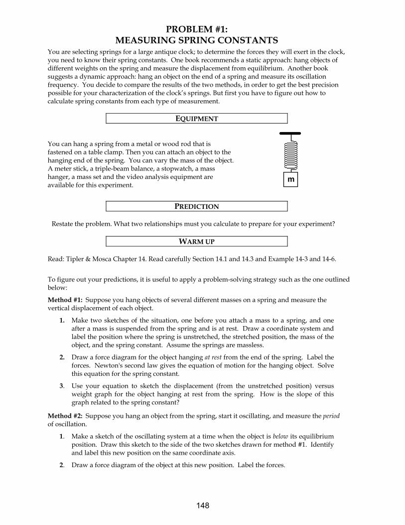
Problem #1: Measuring Spring Constants 148

Problem #2: The Effective Spring Constant 151

Problem #3: Oscillation Frequency with Two Springs 154

Problem #4: Oscillation Frequency of an Extended System 156

Problem #5: Driven Oscillations 159


Laboratory VIII Cover Sheet 163

Appendix A: Significant Figures 165

Appendix B: Accuracy, Precision, and Uncertainty 169

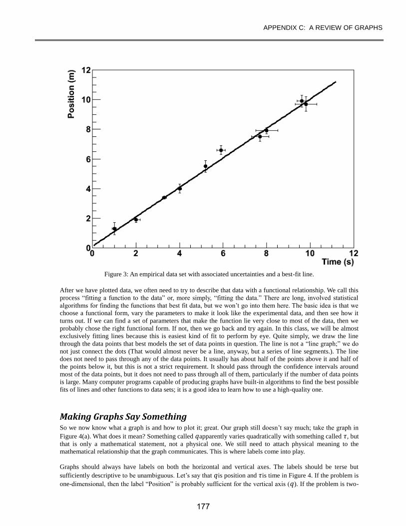
Appendix C: A Review of Graphs 175

Appendix D: Video Analysis of Motion 183

Appendix F: A Guide to Writing Lab Reports 193

Appendix G: Sample Lab Report 201

2

Acknowledgments

Much of the work to develop this problem solving laboratory was supported by the

University of Minnesota and the National Science Foundation. We would like to

thank all the people who have contributed directly to the development of this

laboratory manual:

Sean Albiston Heather Brown Jennifer Docktor

Andy Ferstl Tom Foster Kaiyan Gao

Charles Henderson Ted Hodapp Tao Hu

Andrew Kunz Vince Kuo Roman Lutchyn

Laura McCullough Michael Myhrom Maribel Núñez V.

Jeremy Paschke Leon Steed Tom Thaden-Koch

Hao Wang Sean Albiston

And all of the faculty and graduate students who helped to find the 'bugs' in these

instructions.

Kenneth & Patricia Heller

Kenneth Heller & Patricia Heller

3

4

WELCOME TO THE PHYSICS LABORATORY

Physics is our human attempt to explain the workings of the world. The success of that attempt is evident in the technology of our society. You have already developed your own physical theories to understand the world around you. Some of these ideas are consistent with accepted theories of physics while others are not. This laboratory manual is designed, in part, to help you recognize where your ideas agree with those accepted by physics and where they do not. It is also designed to help you become a better physics problem solver. You are presented with contemporary physical theories in lecture and in your textbook. In the laboratory you can apply the theories to real-world problems by comparing your application of those theories with reality. You will clarify your ideas by: answering questions and solving problems before you come to the lab room, performing experiments and having discussions with classmates in the lab room, and occasionally by writing lab reports after you leave. Each laboratory has a set of problems that ask you to make decisions about the real world. As you work through the problems in this laboratory manual, remember: the goal is not to make lots of measurements. The goal is for you to examine your ideas about the real world. The three components of the course - lecture, discussion section, and laboratory section - serve different purposes. The laboratory is where physics ideas, often expressed in mathematics, meet the real world. Because different lab sections meet on different days of the week, you may deal with concepts in the lab before meeting them in lecture. In that case, the lab will serve as an introduction to the lecture. In other cases the lecture will be a good introduction to the lab. The amount you learn in lab will depend on the time you spend in preparation before coming to lab. Before coming to lab each week you must read the appropriate sections of your text, read the assigned problems to develop a fairly clear idea of what will be happening, and complete the prediction and method questions for the assigned problems. Often, your lab group will be asked to present its predictions and data to other groups so that everyone can participate in understanding how specific measurements illustrate general concepts of physics. You should always be prepared to explain your ideas or actions to others in the class. To show your instructor that you have made the appropriate connections between your measurements and the basic physical concepts, you will be asked to write a laboratory report. Guidelines for preparing lab reports can be found in the lab manual appendices and in this introduction. An example of a good lab report is shown in Appendix E. Please do not hesitate to discuss any difficulties with your fellow students or the lab instructor. Relax. Explore. Make mistakes. Ask lots of questions, and have fun.

5

INTRODUCTION

WHAT TO DO TO BE SUCCESSFUL IN THIS LAB:

Safety comes first in any laboratory. If in doubt about any procedure, or if it seems unsafe to you, STOP. Ask your lab instructor for help.

A. What to bring to each laboratory session:

1. Bring an 8" by 10" graph-ruled lab journal, to all lab sessions. Your journal is your "extended memory" and should contain everything you do in the lab and all of your thoughts as you are going along. Your lab journal is a legal document; you should never tear pages from it. Your lab journal must be bound (as University of Minnesota 2077-S) and must not allow pages to be easily removed (as spiral bound notebooks).

2. Bring a "scientific" calculator.

3. Bring this lab manual.

B. Prepare for each laboratory session:

Each laboratory consists of a series of related problems that can be solved using the same basic concepts and principles. Sometimes all lab groups will work on the same problem, other times groups will work on different problems and share results.

1. Before beginning a new lab, carefully read the Introduction, Objectives and Preparation

sections. Read sections of the text specified in the Preparation section. 2. Each lab contains several different experimental problems. Before you come to a lab,

complete the assigned Prediction and Method Questions. The Method Questions help you build a prediction for the given problem. It is usually helpful to answer the Method Questions before making the prediction. These individual predictions will be checked (graded) by your lab instructor immediately at the beginning of each lab session. This preparation is crucial if you are going to get anything out of your laboratory work. There are at least two other reasons for preparing:

a) There is nothing duller or more exasperating than plugging mindlessly into a procedure

you do not understand. b) The laboratory work is a group activity where every individual contributes to the

thinking process and activities of the group. Other members of your group will be unhappy if they must consistently carry the burden of someone who isn't doing his/her share.

C. Laboratory Reports

At the end of every lab (about once every two weeks) you will be assigned to write up one of the experimental problems. Your report must present a clear and accurate account of what you and your group members did, the results you obtained, and what the results mean. A report must

6

INTRODUCTION

not be copied or fabricated. (That would be scientific fraud.) Copied or fabricated lab reports will be treated in the same manner as cheating on a test, and will result in a failing grade for the course and possible expulsion from the University. Your lab report should describe your predictions, your experiences, your observations, your measurements, and your conclusions. A description of the lab report format is discussed at the end of this introduction. Each lab report is due, without fail, within two days of the end of that lab.

D. Attendance

Attendance is required at all labs without exception. If something disastrous keeps you from your scheduled lab, contact your lab instructor immediately. The instructor will arrange for you to attend another lab section that same week. There are no make-up labs in this course.

E. Grades

Satisfactory completion of the lab is required as part of your course grade. Those not completing all lab assignments by the end of the quarter at a 60% level or better will receive a quarter grade of F for the entire course. The laboratory grade makes up 15% of your final course grade. Once again, we emphasize that each lab report is due, without fail, within two days of the end of that lab.

There are two parts of your grade for each laboratory: (a) your laboratory journal, and (b) your formal problem report. Your laboratory journal will be graded by the lab instructor during the laboratory sessions. Your problem report will be graded and returned to you in your next lab session. If you have made a good-faith attempt but your lab report is unacceptable, your instructor may allow you to rewrite parts or all of the report. A rewrite must be handed in again within two days of the return of the report to you by the instructor.

F. The laboratory class forms a local scientific community. There are certain basic rules for

conducting business in this laboratory. 1. In all discussions and group work, full respect for all people is required. All

disagreements about work must stand or fall on reasoned arguments about physics principles, the data, or acceptable procedures, never on the basis of power, loudness, or intimidation.

2. It is OK to make a reasoned mistake. It is in fact, one of the most efficient ways to learn.

This is an academic laboratory in which to learn things, to test your ideas and predictions by

collecting data, and to determine which conclusions from the data are acceptable and reasonable to other people and which are not.

What do we mean by a "reasoned mistake"? We mean that after careful consideration and after a substantial amount of thinking has gone into your ideas you simply give your best prediction or explanation as you see it. Of course, there is always the possibility that your idea does not accord with the accepted ideas. Then someone says, "No, that's not the way I see it and here's why." Eventually persuasive evidence will be offered for one viewpoint or the other. "Speaking out" your explanations, in writing or vocally, is one of the best ways to learn.

7

INTRODUCTION

3. It is perfectly okay to share information and ideas with colleagues. Many kinds of help are okay. Since members of this class have highly diverse backgrounds, you are encouraged to help each other and learn from each other.

However, it is never okay to copy the work of others. Helping others is encouraged because it is one of the best ways for you to learn, but copying

is inappropriate and unacceptable. Write out your own calculations and answer questions in your own words. It is okay to make a reasoned mistake; it is wrong to copy.

No credit will be given for copied work. It is also subject to University rules about plagiarism and cheating, and may result in dismissal from the course and the University. See the University course catalog for further information.

4. Hundreds of other students use this laboratory each week. Another class probably follows directly

after you are done. Respect for the environment and the equipment in the lab is an important part of making this experience a pleasant one.

The lab tables and floors should be clean of any paper or "garbage." Please clean up your area before you leave the lab. The equipment must be either returned to the lab instructor or left neatly at your station, depending on the circumstances.

A note about Laboratory equipment: At times equipment in the lab may break or may be found to be broken. If this happens you should inform your TA and report the problem to the equipment specialist by sending an email to: [email protected] Describe the problem, including any identifying aspects of the equipment, and be sure to include your lab room number. If equipment appears to be broken in such a way as to cause a danger do not use the equipment and inform your TA immediately.

In summary, the key to making any community work is RESPECT. Respect yourself and your ideas by behaving in a professional manner at all times. Respect your colleagues (fellow students) and their ideas. Respect your lab instructor and his/her effort to provide you with an environment in which you can learn. Respect the laboratory equipment so that others coming after you in the laboratory will have an appropriate environment in which to learn.

8

LABORATORY 0: DETERMINING AN EQUATION FROM A GRAPH

Throughout this course, you will use computer programs to graph physical quantities. Before measuring, you enter equations to represent predictions for the quantities to be measured. After measuring, you determine the equations that best represent (fit) the measured data, and compare the resulting Fit Equations with your Prediction Equations. This activity will familiarize you with the procedure for fitting equations to measured data.

EXPLORATION Log on to the computer. Open the PracticeFit program by double-clicking its icon on the desktop. The “Instruction” box provides instructions that change as you progress. Holding the mouse over a button or the graph also provides some help. You will try to fit equations to data generated by a Mystery Function. There are several sets of “Mystery Functions” to choose from; ranging from simpler (1) to more varied and complicated (10). The parameters, and in some cases the function types, are randomly chosen; you can try each Mystery Function several times until you are comfortable with it. Follow the instructions on the screen until you are asked to select a “Fit Function” to approximate the Mystery Function data graphed on the screen. (You may need to change the graph’s axis limits to locate the Mystery Function data!) The curve graphed for the Fit Function will change to match parameters you select; try to find the equation that gives the best possible fit to the Mystery Function data. The Warm Up Questions below are designed to help. Once you are satisfied with an equation, press “Accept Fit Function” to reveal the equation of the Mystery Function.

WARM UP The following questions should help you determine the equation that best matches the curve:

1. Determine the type of Fit Function that can best approximate the Mystery Function data. Examine the data’s graph. Is it a straight line? If the graph bends, does it have a parabolic shape, an exponential shape, or a repeating pattern? Use your knowledge of functions to select the best equation type from the choices offered by PracticeFit.

2. Next you need to determine the constants in the equation. Examine the graph where the horizontal coordinate is zero:

At this point, what is the value of the vertical coordinate of the graph? What constant in the Fit Function equation is represented by this vertical coordinate?

At this same point, what is the slope of the graph, and what constant does it represent? (If you have taken some calculus, you will know that the derivative of a function represents the slope of its graph.)

If there are more constant parameters to determine for the Fit Function, you must look at other points on the graph; your knowledge of functions and calculus will help. You might examine points on the horizontal axis, points with zero slope, and/or the graph’s asymptotic behavior. It may also be useful to consider the derivative of the Fit Function.

During the rest of this physics course, you will deal with real physical situations. You can usually determine the form of the best Fit Function and estimate its constant parameters based on your physics knowledge and what you observe in the laboratory; this can greatly simplify the fitting process.

9

LAB 0: PRACTICE FIT

CONCLUSION

How close was your equation to the Mystery Function used to generate the each curve? If your equation was not exactly the same as the actual equation, how would you determine what would be an acceptable degree of difference? If the horizontal axis represents time and the vertical axis represents position, what type of motion might this curve represent?

10

LABORATORY I:

DESCRIPTION OF MOTION IN ONE DIMENSION

In this laboratory you will measure and analyze one-dimensional motion; that is, motion along a straight line.

With digital videos, you will measure the positions of moving objects at regular time intervals. You will

investigate relationships among quantities useful for describing objects’ motion. Determining these

kinematics quantities (position, time, velocity, and acceleration) under different conditions allows you to

develop an intuition about relationships among them. In particular, you should identify which relationships

are only valid in some situations and which apply to all situations.

There are many possibilities for one-dimensional motion of an object. It might move at a constant speed,

speed up, slow down, or exhibit some combination of these. When making measurements, you must quickly

understand your data to decide if the results make sense. If they don't make sense to you, then you have not

set up the situation properly to explore the physics you desire, you are making measurements incorrectly, or

your ideas about the behavior of objects in the physical world are incorrect. In any of the above cases, it is a

waste of time to continue making measurements. You must stop, determine what is wrong, and fix it.

If your ideas are wrong, this is your chance to correct them by discussing the inconsistencies with your

partners, rereading your text, or talking with your instructor. Remember, one of the reasons for doing

physics in a laboratory setting is to help you confront and overcome your incorrect ideas about physics,

measurements, calculations, and technical communications. Pinpointing and working on your own

difficulties will help you in other parts of this physics course, and perhaps in other courses. Because people

are faster at recognizing patterns in pictures than in numbers, the computer will graph your data as you go

along.

OBJECTIVES:

After you successfully complete this laboratory, you should be able to:

Describe completely the motion of any object moving in one dimension using position, time, velocity, and acceleration.

Distinguish between average quantities and instantaneous quantities for the motion of an object.

Write the mathematical relationships among position, time, velocity, average velocity, acceleration, and average acceleration for different situations.

Graphically analyze the motion of an object.

Begin using technical communication skills such as keeping a laboratory journal and writing a laboratory report.

11

LAB I: INTRODUCTION

PREPARATION:

Read Tipler & Mosca: Chapter 2. Also read Appendix D, the instructions for doing video analysis. Before

coming to the lab you should be able to:

Define and recognize the differences among these concepts: - Position, displacement, and distance. - Instantaneous velocity and average velocity. - Instantaneous acceleration and average acceleration.

Find the slope and intercept of a straight-line graph. If you need help, see Appendix C.

Determine the slope of a curve at any point on that curve. If you need help, see Appendix C.

Determine the derivative of a quantity from the appropriate graph.

Use the definitions of sin θ, cos θ, and tan θ for a right triangle.

12

PROBLEM #1: CONSTANT VELOCITY MOTION

Since this physics laboratory design may be new to you, this first problem, and only this one, contains both the instructions to explore constant velocity motion and an explanation of the various parts of the instructions. The explanation of the instructions is preceded by the double, vertical lines seen to the left. These laboratory instructions may be unlike any you have seen before. You will not find worksheets or step-by-step instructions. Instead, each laboratory consists of a set of problems that you solve before coming to the laboratory by making an organized set of decisions (a problem solving strategy) based on your initial knowledge. The prediction and warm up questions are designed to help you examine your thoughts about physics. These labs are your opportunity to compare your ideas about what "should" happen with what really happens. The labs will have little value in helping you learn physics unless you take time to predict what will happen before you do something. While in the laboratory, take your time and try to answer all the questions in this lab manual. In particular, answering each of the exploration questions can save you time and frustration later by helping you understand the behavior and limitations of your equipment before you make measurements. Make sure to complete the laboratory problem, including all analysis and conclusions, before moving on to the next one.

The first paragraphs of each lab problem describe a real-world situation. Before coming to lab, you will solve a physics problem to predict something about that situation. The measurements and analysis you perform in lab will allow you to test your prediction against the behavior of the real world. You have an internship managing a network of closed-circuit “Freeway cameras” for MnDOT Metro Traffic Engineering. Your boss wants to use images from those cameras to determine velocities of cars, particularly during unusual circumstances such as traffic accidents. Your boss knows that you have taken physics and asks you to prepare a presentation. During the presentation, you must demonstrate possibilities for determining a car’s average velocity from graphs of its position vs. time, instantaneous velocity vs. time, and instantaneous acceleration vs. time. You decide to model the situation with a small digital camera and a toy car that moves at a constant velocity.

EQUIPMENT This section contains a brief description of the apparatus you can use to test your prediction. Working through the exploration section will familiarize you with the details.

For this problem, you will use a motorized toy car, which moves with a constant velocity on an aluminum track. You will also have a stopwatch, a meter stick, a video camera and a computer with video analysis applications written in LabVIEW (VideoRECORDER and MotionLab, described in Appendix D) to help you analyze the motion. If equipment is missing or broken, please submit a problem report by sending an email to [email protected]. Please include the room number and brief description of the problem. If you are unable to, please ask your TA to submit a problem report.

PREDICTION Everyone has "personal theories" about the way the world works. One purpose of this lab is to help you clarify your conceptions of the physical world by testing the predictions of your personal theory against what really happens. For this reason, you will always predict what will happen before collecting and analyzing the data. Your prediction should be completed and written in your lab

13


journal before you come to lab. The “Warm Up Questions” in the next section are designed to help you make your prediction and should also be completed before you come to lab. This may seem a little backwards. Although the “Prediction” section appears before the warm up questions, you should complete the warm up questions before making the prediction. The “Prediction” section merely helps you identify the goal of the lab problem.

Spend the first few minutes at the beginning of the lab session comparing your prediction with those of your partners. Discuss the reasons for differences in opinion. It is not necessary that your predictions are correct, but it is absolutely crucial that you understand the basis of your prediction.

Sketch graphs of position vs. time, instantaneous velocity vs. time, and instantaneous acceleration vs. time for the toy car. How could you determine the speed of the car from each graph? Sometimes your prediction is an "educated guess" based on your knowledge of the physical world. In these problems exact calculation is too complicated and is beyond this course. However, for every problem it’s possible to come up with a qualitative prediction by making some plausible simplifications. For other problems, you will be asked to use your knowledge of the concepts and principles of physics to calculate a mathematical relationship between quantities in the experimental problem.

WARM UP

Warm Up Questions are a series of questions intended to help you solve the problem stated in the opening paragraphs. They may help you make the prediction, help you plan how to analyze data, or help you think through the consequences of a prediction that is an educated guess. Warm Up questions should be answered and written in your lab journal before you come to lab.

Read: Tipler & Mosca Chapter 2. Sections 2.1-2.2 To find schemes for determining a car’s velocity, you need to think about representing its motion. The following questions should help.

1. How would you expect an instantaneous velocity vs. time graph to look for an object with constant velocity? Make a rough sketch and explain your reasoning. Assign appropriate labels and units to your axes. Write an equation that describes this graph. What is the meaning of each quantity in your equation? In terms of the quantities in your equation, what is the velocity?

2. How would you expect an instantaneous acceleration vs. time graph to look for an object moving with a constant velocity? Make a rough sketch and explain your reasoning. Remember axis labels and units. Write down an equation that describes this graph. In this case, what can you say about the velocity?

3. How would you expect a position vs. time graph to look for an object moving with constant velocity? Make a rough sketch and explain your reasoning. What is the relationship between this graph and the instantaneous velocity versus time graph? Write down an equation that describes this graph. What is the meaning of each quantity in your equation? In terms of the quantities in your equation, what is the velocity?

14


EXPLORATION

This section is extremely important—many instructions will not make sense, or you may be led astray, if you fail to carefully explore your experimental plan. In this section you practice with the apparatus and carefully observe the behavior of your physical system before you make precise measurements. You will also explore the range over which your apparatus is reliable. Remember to always treat the apparatus with care and respect. Students in the next lab section will use the equipment after you are finished with it. If you are unsure about how equipment works, ask your lab instructor. If at any time during the course of this lab you find a piece of equipment is broken, please submit a problem report by sending an email to [email protected]. Most equipment has a range in which its operation is simple and straightforward. This is called its range of reliability. Outside that range, complicated corrections are needed. Be sure your planned measurements fall within the range of reliability. You can quickly determine the range of reliability by making qualitative observations at the extremes of your measurement plan. Record these observations in your lab journal. If the apparatus does not function properly for the ranges you plan to measure, you should modify your plan to avoid the frustration of useless measurements. At the end of the exploration you should have a plan for doing the measurements that you need. Record your measurement plan in your journal. This exploration section is much longer than most. You will record and analyze digital videos several times during the semester.

Place one of the metal tracks on your lab bench and place the toy car on the track. Turn on the car and observe its motion. Qualitatively determine if it actually moves with a constant velocity. Use the meter stick and stopwatch to determine the speed of the car. Estimate the uncertainty in your speed measurement. Turn on the video camera and look at the motion as seen by the camera on the computer screen. Go to Appendix D for instructions about using the VideoRECORDER software. Do you need to focus the camera to get a clean image? Each camera has an adjustable focus by turning the lens, make sure yours is working correctly. Move the camera closer to the car. How does this affect the video image? Try moving it farther away. Raise the height of the camera tripod. How does this affect the image? Decide where you want to place the camera to get the most useful image. Practice taking videos of the toy car. You will make and analyze many videos in this course! Write down the best situation for taking a video in your journal for future reference. When you have a good movie, make sure to save it in the Lab Data folder on the desktop. Quit VideoRECORDER and open MotionLab to analyze your movie. Although the directions to analyze a video are given during the procedure in a box with the title “INSTRUCTIONS”, the following is a short summary of them that will be useful to do the exploration for this and any other lab video (for more reference you should read at least once the Appendix D). 1. Open the video that you are interested in by clicking the “AVI” button.

15


2. Advance the video with the “Fwd >” button to the frame where the first data point will be

taken, then select “Accept” from the main controls. This step is very important because it sets up the origin of your time axis (t=0).

3. To tell the analysis program the real size of the video images, select some object in the plane

of motion that you can measure. Drag the red cursor, located in the center of the video display, to one end of the calibration object. Click “Accept” button when the red cursor is in place. Move the red cursor to the other end and select “Accept”. Enter the length of the object in the “Length” box and specify the “Units”. Select the “Accept” button again, then select the “Quit Calibration” button to exit the calibration routine.

4. Enter your prediction equations of how you expect the position to behave. Notice that the

symbols used by the equations in the program are dummy letters, which means that you have to identify those with the quantities involved in your prediction. In order to do the best guess you will need to take into account the scale and the values from your practice trials using the stopwatch and the meter stick. Once your x-position prediction is ready, select “Accept” in the main controls. Repeat the previous procedure for the y-position.

5. Once both your x and y position predictions are entered, the data collection routine will

begin. Select a specific point on the object whose motion you are analyzing. Drag the red cursor over this point and click the “Add Point” button from the data acquisition controls and you will see the data on the appropriate graph on your computer screen, after this the video will advance one frame. Again, drag the green cursor over the selected spot on the object and select ”Add Point.” Keep doing this until you have enough data, then select “Quit Data Acq”.

6. Decide which equation and constants are the best approximations for your data, then select

“Accept” from the main controls. 7. At this level the program will ask you to enter your predictions for velocity in x- and y-

directions. Choose the appropriate equations and give your best approximations for the constants. Once you have accepted your vx - and vy –predictions, you will see the data on the last two graphs.

8. Fit your data for these velocities in the same way that you did for position. Accept your fit

and click the “Print” button to get a hard copy of your graphs.

Now you are ready to answer some questions that will be helpful for planning your measurements.

What would happen if you calibrate with an object that is not on the plane of the motion?

What would happen if you use different points on your car to get your data points?

MEASUREMENT

Now that you have predicted the result of your measurement and have explored how your apparatus behaves, you are ready to make careful measurements. To avoid wasting time and effort, make the minimal measurements necessary to convince yourself and others that you have solved the laboratory problem.

16


1. Record the time the car takes to travel a known distance. Estimate the uncertainty in time and distance measurements. 2. Take a good video of the car’s motion. Analyze the video with MotionLab to predict and fit functions for position vs. time and velocity vs. time. If possible, every member of your group should analyze a video. Record your procedures, measurements, prediction equations, and fit equations in a neat and organized manner so that you can understand them a month from now. Some future lab problems will require results from earlier ones.

ANALYSIS Data by itself is of very limited use. Most interesting quantities are those derived from the data, not direct measurements themselves. Your predictions may be qualitatively correct but quantitatively very wrong. To see this you must process your data. Always complete your data processing (analysis) before you take your next set of data. If something is going wrong, you shouldn't waste time taking a lot of useless data. After analyzing the first data, you may need to modify your measurement plan and re-do the measurements. If you do, be sure to record the changes in your plan in your journal.

Calculate the average speed of the car from your stopwatch and meter stick measurements. Determine if the speed is constant within your measurement uncertainties. As you analyze data from a video, be sure to write down each of the prediction and fit equations for position and velocity. When you have finished making a fit equation for each graph, rewrite the equations in a table but now matching the dummy letters with the appropriate kinetic quantities. If you have constant values, assign them the correct units.

CONCLUSIONS After you have analyzed your data, you are ready to answer the experimental problem. State your result in the most general terms supported by your analysis. This should all be recorded in your journal in one place before moving on to the next problem assigned by your lab instructor. Make sure you compare your result to your prediction.

Compare the car’s speed measured with video analysis to the measurement using a stopwatch. Did your measurements and graphs agree with your answers to the Warm Up Questions? If not, why? Do your graphs match what you expected for constant velocity motion? What are the limitations on the accuracy of your measurements and analysis?

17

PROBLEM #2: MOTION DOWN AN INCLINE

You have a job working with a team studying accidents for the state safety board. To investigate one accident, your team needs to determine the acceleration of a car rolling down a hill without any brakes. Everyone agrees that the car’s velocity increases as it rolls down the hill but your team’s supervisor believes that the car's acceleration also increases uniformly as it rolls down the hill. To test your supervisor’s idea, you determine the acceleration of a cart as it moves down an inclined track in the laboratory.

EQUIPMENT For this problem you will have a stopwatch, a meter stick, an end stop, a wood block, a video camera and a computer with a video analysis application written in LabVIEW (VideoRECORDER and MotionLab applications.) You will also have a cart to roll down an inclined track. If you have broken or missing equipment, submit a problem report by sending an email to [email protected] – please include the room # and a brief description of the problem.

PREDICTION Consider the questions printed in italics, below, to make a rough sketch of how you expect the acceleration vs. time graph to look for a cart under the conditions given in the problem. Explain your reasoning. Do you think the cart's acceleration changes as it moves down the track? If so, how does the acceleration change (increase or decrease)? Or, do you think the acceleration is constant (does not change) as the cart moves down the track?

WARM UP Read: Tipler & Mosca Chapter 2. Sections 2.1-2.3 The following questions should help you to explore three different scenarios involving the physics given in the problem.

1. How would you expect an instantaneous acceleration vs. time graph to look for a cart moving with a constant acceleration? With a uniformly increasing acceleration? With a uniformly decreasing acceleration? Make a rough sketch of the graph for each possibility and explain your reasoning. To make the comparison easier, it is useful to draw these graphs next to each other. Remember to assign labels and units to your axes. Write down an equation for each graph. Explain what the symbols in each of the equations mean. What quantities in these equations can you determine from your graph?

2. Write down the relationship between the acceleration and the velocity of the cart. Use that

relationship to construct an instantaneous velocity versus time graph just below each of your acceleration versus time graphs from question 1, with the same scale for each time axis. Write down an equation for each graph. Explain what the symbols in each of the equations mean. What quantities in these equations can you determine from your graph?

3. Write down the relationship between the velocity and the position of the cart. Use that

relationship to construct a position versus time graph just below each of your velocity versus time graphs from question 2, with the same scale for each time axis. Write down

18


an equation for each graph. Explain what the symbols in each of the equations mean. What quantities in these equations can you determine from your graph?

EXPLORATION

In order to have an incline you will use the wood block and the aluminum track. This set up will give you an angle with respect to the table. How are you going to measure this angle? Hint: Think trigonometry! Start with a small angle and with the cart at rest near the top of the track. Observe the cart as it moves down the inclined track. Try a range of angles. BE SURE TO CATCH THE CART BEFORE IT HITS THE END STOP! If the angle is too large, you may not get enough video frames, and thus enough position and time measurements, to measure the acceleration accurately. If the angle is too small the acceleration may be too small to measure accurately with the precision of your measuring instruments. Select the best angle for this measurement. Where is the best place to release the cart so it does not damage the equipment but has enough of its motion captured on video? Be sure to catch the cart before it collides with the end stop. When placing the camera, consider which part of the motion you wish to capture. Try different camera positions until you get the best possible video. Make sure you have a good object in your video to calibrate with. Hint: Your video may be easier to analyze if the motion on the video screen is purely horizontal. Why? It could be useful to rotate the camera! What is the total distance through which the cart rolls? How much time does it take? These measurements will help you set up the graphs for your computer data taking. You may wish to follow the steps given in the “Exploration” section of problem 1 to work with your video. Write down your measurement plan.

MEASUREMENT Follow the measurement plan you wrote down. When you have finished making measurements, you should have printouts of position and velocity graphs and good records (including uncertainty) of: your determination of the incline angle, the time it takes the cart to roll a known distance down the incline starting from rest, the length of the cart, and prediction and fit equations for position and velocity. Make sure that every one gets the chance to operate the computer. Record all of your measurements; you may be able to re-use some of them in other lab problems. Note: Be sure to record your measurements with the appropriate number of significant figures (see Appendix A) and with your estimated uncertainty (see Appendix B). Otherwise, the data is nearly meaningless.

19


ANALYSIS

Calculate the cart’s average acceleration from the distance and time measurements you made with a meter stick and stopwatch. Look at your graphs and rewrite all of the equations in a table but now matching the dummy letters with the appropriate kinetic quantities. If you have constant values, assign them the correct units, and explain their meaning. From the velocity vs. time graph, determine if the acceleration is constant, increasing, or decreasing as the cart goes down the ramp. Use the function representing the velocity vs. time graph to calculate the acceleration of the cart as a function of time. Make a graph of that function. Is the average acceleration of the cart equal to its instantaneous acceleration in this case? Compare the accelerations for the cart you found with your video analysis to your acceleration measurement using a stopwatch.

CONCLUSION How do the graphs of your measurements compare to your predictions? Was your boss right about how a cart accelerates down a hill? If yes, state your result in the most general terms supported by your analysis. If not, describe how you would convince your boss of your conclusions. What are the limitations on the accuracy of your measurements and analysis?

20

PROBLEM #3: MOTION UP AND DOWN AN INCLINE

A proposed ride at the Valley Fair amusement park launches a roller coaster car up an inclined track. Near the top of the track, the car reverses direction and rolls backwards into the station. As a member of the safety committee, you have been asked to describe the acceleration of the car throughout the ride. The launching mechanism has been well tested. You are only concerned with the roller coaster’s trip up and back down. To test your expectations, you decide to build a laboratory model of the ride.

EQUIPMENT For this problem you will have a stopwatch, a meter stick, an end stop, a wood block, a video camera and a computer with a video analysis application written in LabVIEW (VideoRECORDER and MotionLab applications). You will also have a cart to roll up an inclined track. If you have broken or missing equipment, submit a problem report by sending an email to [email protected] – please include the room # and a brief description of the problem.

PREDICTION Make a rough sketch of how you expect the acceleration vs. time graph to look for a cart with the conditions discussed in the problem. The graph should be for the entire motion of going up the track, reaching the highest point, and then coming down the track. Do you think the acceleration of the cart moving up an inclined track will be greater than, less than, or the same as the acceleration of the cart moving down the track? What is the acceleration of the cart at its highest point? Explain your reasoning.

WARM UP Read: Tipler & Mosca Chapter 2. Sections 2.1-2.3 The following questions should help you examine the consequences of your prediction.

1. Sketch a graph of the instantaneous acceleration vs. time graph you expect for the cart as it rolls up and then back down the track after an initial push. Sketch a second instantaneous acceleration vs. time graph for a cart moving up and then down the track with the direction of a constant acceleration always down along the track after an initial push. On each graph, label the instant where the cart reverses its motion near the top of the track. Explain your reasoning for each graph. Write down the equation(s) that best represents each graph. If there are constants in your equations, what kinematics quantities do they represent? How would you determine these constants from your graphs?

2. Write down the relationship between the acceleration and the velocity of the cart. Use that relationship to construct an instantaneous velocity vs. time graph just below each of acceleration vs. time graph from question 1, with the same scale for each time axis. (The connection between the derivative of a function and the slope of its graph will be useful.) On each graph, label the instant where the cart reverses its motion near the top of the track. Write an equation for each graph. If there are constants in your equations, what kinematics quantities do they represent? How would you determine these constants from your graphs? Can any of the constants be determined from the constants in the equation representing the acceleration vs. time graphs?

21


3. Write down the relationship between the velocity and the position of the cart. Use that relationship to construct an instantaneous position vs. time graph just below each of your velocity vs. time graphs from question 2, with the same scale for each time axis. (The connection between the derivative of a function and the slope of its graph will be useful.) On each graph, label the instant where the cart reverses its motion near the top of the track. Write down an equation for each graph. If there are constants in your equations, what kinematics quantities do they represent? How would you determine these constants from your graphs? Can any of the constants be determined from the constants in the equations representing velocity vs. time graphs?

4. Which graph do you think best represents how position of the cart will change with time? Adjust your prediction if necessary and explain your reasoning.

EXPLORATION

What is the best way to change the angle of the inclined track in a reproducible way? How are you going to measure this angle with respect to the table? (Think about trigonometry.) Start the cart up the track with a gentle push. BE SURE TO CATCH THE CART BEFORE IT HITS THE END STOP ON ITS WAY DOWN! Observe the cart as it moves up the inclined track. At the instant the cart reverses direction, what is its velocity? Its acceleration? Observe the cart as it moves down the inclined track. Do your observations agree with your prediction? If not, discuss it with your group. Where is the best place to put the camera? Which part of the motion do you wish to capture? Try different angles. Be sure to catch the cart before it collides with the end stop at the bottom of the track. If the angle is too large, the cart may not go up very far and will give you too few video frames for the measurement. If the angle is too small it will be difficult to measure the acceleration. Take a practice video and play it back to make sure you have captured the motion you want (see the “Exploration” section in Problem 1, and appendix D, for hints about using the camera and VideoRECORDER / MotionLab.) Hint: To analyze motion in only one dimension (like in the previous problem) rather than two dimensions, it could be useful to rotate the camera! What is the total distance through which the cart rolls? Using your stopwatch, how much time does it take? These measurements will help you set up the graphs for your computer data taking, and can provide for a check on your video analysis of the cart’s motion. Write down your measurement plan.

MEASUREMENT Follow your measurement plan to make a video of the cart moving up and then down the track at your chosen angle. Record the time duration of the cart’s trip, and the distance traveled. Make sure you get enough points for each part of the motion to determine the behavior of the acceleration. Don't forget to measure and record the angle (with estimated uncertainty). Work through the complete set of calibration, prediction equations, and fit equations for a single (good) video before making another video. Make sure everyone in your group gets the chance to operate the computer.

22


ANALYSIS

From the time given by the stopwatch and the distance traveled by the cart, calculate its average acceleration. Estimate the uncertainty. Look at your graphs and rewrite all of the equations in a table but now matching the dummy letters with the appropriate kinetic quantities. If you have constant values, assign them the correct units, and explain their meaning. Can you tell from your graph where the cart reaches its highest point? From the velocity vs. time graph determine if the acceleration changes as the cart goes up and then down the ramp. Use the function representing the velocity vs. time graph to calculate the acceleration of the cart as a function of time. Make a graph of that function. Can you tell from this instantaneous acceleration vs. time graph where the cart reaches its highest point? Is the average acceleration of the cart equal to its instantaneous acceleration in this case? Compare the acceleration function you just graphed with the average acceleration you calculated from the time on the stopwatch and the distance the cart traveled.

CONCLUSION How do your position vs. time, velocity vs. time graphs compare with your answers to the warm up questions and the prediction? What are the limitations on the accuracy of your measurements and analysis? Did the cart have the same acceleration throughout its motion? Did the acceleration change direction? Was the acceleration zero at the top of its motion? Describe the acceleration of the cart through its entire motion after the initial push. Justify your answer with kinematics arguments and experimental results. If there are any differences between your predictions and your experimental results, describe them and explain why they occurred.

23

PROBLEM #4: MOTION DOWN AN INCLINE WITHAN INITIAL VELOCITY

Because of your physics background, you have a summer job with a company that is designing a new bobsled for the U.S. team to use in the next Winter Olympics. You know that the success of the team depends crucially on the initial push of the team members – how fast they can push the bobsled before they jump into the sled. You need to know in more detail how that initial velocity affects the motion of the bobsled. In particular, your boss wants you to determine if the initial velocity of the sled affects its acceleration down the ramp. To solve this problem, you decide to model the situation using a cart moving down an inclined track.

EQUIPMENT You will have a stopwatch, a meter stick, an end stop, a wood block, a video camera and a computer with a video analysis application written in LabVIEW. You will also have a cart to roll down an inclined track. If you have broken or missing equipment, submit a problem report by sending an email to [email protected] – please include the room # and a brief description of the problem.

PREDICTION Do you think the cart launched down the inclined track will have a larger acceleration, smaller acceleration, or the same acceleration as the cart released from rest?

WARM UP Read: Tipler & Mosca Chapter 2. Read carefully Section 2.3 and Examples 2-9 & 2-13. The following questions should help you (a) understand the consequences of your prediction and (b) interpret your measurements.

1. Sketch a graph of instantaneous acceleration vs. time graph when the cart rolls down the track after an initial push (your graph should begin after the initial push.) Compare this to an instantaneous acceleration vs. time graph for a cart released from rest. (To make the comparison easier, draw the graphs next to each other.) Explain your reasoning for each graph. Write down the equation(s) that best represents each of the graphs. If there are constants in your equations, what kinematics quantities do they represent? How would you determine the constants from your graphs?

2. Write down the relationship between the acceleration and the velocity of the cart. Use that relationship to construct an instantaneous velocity vs. time graph, after an initial push, just below each of your acceleration vs. time graphs from question 1. Use the same scale for your time axes. (The connection between the derivative of a function and the slope of its graph will be useful.) Write down the equation that best represents each graph. If there are constants in your equations, what kinematics quantities do they represent? How would you determine the constants from your graphs? Can any of the constants be determined from the equations representing the acceleration vs. time graphs?

3. Write down the relationship between the velocity and the position of the cart. Use that relationship to construct a position vs. time graph, after an initial push, just below each velocity vs. time graph from question 2. Use the same scale for your time axes. (The connection between the derivative of a function and the slope of its graph will be useful.) Write down the equation that best represents each graph. If there are constants in your equations, what kinematics quantities do they represent? How would you determine

24

PROBLEM #4: MOTION DOWN AN INCLINE WITH NON-ZERO INITIAL VELOCITY

these constants from your graphs? Can any of these constants be determined from the equations representing the velocity vs. time graphs?

EXPLORATION

Slant the track at an angle. (Hint: Is there an angle that would allow you to reuse some of your measurements and calculations from other lab problems?) Determine the best way to gently launch the cart down the track in a consistent way without breaking the equipment. BE SURE TO CATCH THE CART BEFORE IT HITS THE END STOP! Where is the best place to put the camera? Is it important to have most of the motion in the center of the picture? Which part of the motion do you wish to capture? Try taking some videos before making any measurements. What is the total distance through which the cart rolls? How much time does it take? These measurements will help you set up the graphs for your computer data taking. Write down your measurement plan. Make sure everyone in your group gets the chance to operate the camera and the computer.

MEASUREMENT Using the plan you devised in the exploration section, make a video of the cart moving down the track at your chosen angle. Make sure you get enough points for each part of the motion to determine the behavior of the acceleration. Don't forget to measure and record the angle (with estimated uncertainty). Choose an object in your picture for calibration. Choose your coordinate system. Is a rotated coordinate system the easiest to use in this case? Why is it important to click on the same point on the car’s image to record its position? Estimate your accuracy in doing so. Make sure you set the scale for the axes of your graph so that you can see the data points as you take them. Use your measurements of total distance the cart travels and total time to determine the maximum and minimum value for each axis before taking data.

ANALYSIS Choose a function to represent the position vs. time graph. How can you estimate the values of the constants of the function from the graph? You may waste a lot of time if you just try to guess the constants. What kinematics quantities do these constants represent? Choose a function to represent the velocity versus time graph. How can you calculate the values of the constants of this function from the function representing the position versus time graph? Check how well this works. You can also estimate the values of the constants from the graph. Just trying to guess the constants can waste a lot of your time. What kinematics quantities do these constants represent?

25

PROBLEM #4: MOTION DOWN AN INCLINE WITH NON-ZERO INITIAL VELOCITY

From the velocity versus time graph, determine the acceleration as the cart goes down the ramp after the initial push. Use the function representing the velocity versus time graph to calculate the acceleration of the cart as a function of time. Make a graph of that function. As you analyze your video, make sure everyone in your group gets the chance to operate the computer.

CONCLUSIONS Look at the graphs you produced through video analysis. How do they compare to your answers to the warm up questions and your predictions? Explain any differences. What are the limitations on the accuracy of your measurements and analysis? What will you tell your boss? Does the acceleration of the bobsled down the track depend on the initial velocity the team can give it? Does the velocity of the bobsled down the track depend on the initial velocity the team can give it? State your result in the most general terms supported by your analysis.

26

PROBLEM #5: MASS AND MOTION DOWN AN INCLINE

Your neighbors' child has asked for your help in constructing a soapbox derby car. In the soapbox derby, two cars are released from rest at the top of a ramp. The one that reaches the bottom first wins. The child wants to make the car as heavy as possible to give it the largest acceleration. Is this plan reasonable?

EQUIPMENT You will have a stopwatch, a meter stick, an end stop, a wood block, a video camera and a computer with a video analysis application written in LabVIEW. You will also have a cart to roll down an inclined track and additional cart masses to add to the cart. Submit any problems to labhelp.

PREDICTION Do you think that increasing the mass of the cart increases, decreases, or has no effect on the cart’s acceleration?

WARM UP Read: Tipler & Mosca Chapter 2. Read carefully Section 2.3 and Examples 2-9 & 2-13. The following questions should help you (a) understand the consequences of your prediction and (b) interpret your measurements.

1. Make a sketch of the acceleration vs. time graph for a cart released from rest on an inclined track. On the same axes sketch an acceleration vs. time graph for a cart on the same incline, but with a much larger mass. Explain your reasoning. Write down the equations that best represent each of these accelerations. If there are constants in your equations, what kinematics quantities do they represent? How would you determine these constants from your graphs?

2. Write down the relationship between the acceleration and the velocity of the cart. Use that relationship to construct an instantaneous velocity vs. time graph for each case. (The connection between the derivative of a function and the slope of its graph will be useful.) Write down the equation that best represents each of these velocities. If there are constants in your equations, what kinematics quantities do they represent? How would you determine these constants from your graphs? Can any of these constants be determined from the equations representing the accelerations?

3. Write down the relationship between the velocity and the position of the cart. Use that relationship to construct a position vs. time graph for each case. The connection between the derivative of a function and the slope of its graph will be useful. Write down the equation that best represents each of these positions. If there are constants in your equations, what kinematics quantities do they represent? How would you determine these constants from your graphs? Can any of these constants be determined from the equations representing the velocities?

EXPLORATION Slant the track at an angle. (Hint: Is there an angle that would allow you to reuse some of your measurements and calculations from other lab problems?)

27


Observe the motion of several carts of different mass when released from rest at the top of the track. BE SURE TO CATCH THE CART BEFORE IT HITS THE END STOP! From your estimate of the size of the effect, determine the range of mass that will give the best results in this problem. Determine the first two masses you should use for the measurement. How do you determine how many different masses do you need to use to get a conclusive answer? How will you determine the uncertainty in your measurements? How many times should you repeat these measurements? Explain. What is the total distance through which the cart rolls? How much time does it take? These measurements will help you set up the graphs for your computer data taking. Write down your measurement plan. Make sure everyone in your group gets the chance to operate the camera and the computer.

MEASUREMENT Using the plan you devised in the exploration section, make a video of the cart moving down the track at your chosen angle. Make sure you get enough points for each part of the motion to determine the behavior of the acceleration. Don't forget to measure and record the angle (with estimated uncertainty). Choose an object in your picture for calibration. Choose your coordinate system. Is a rotated coordinate system the easiest to use in this case? Why is it important to click on the same point on the car’s image to record its position? Estimate your accuracy in doing so. Make sure you set the scale for the axes of your graph so that you can see the data points as you take them. Use your measurements of total distance the cart travels and the total time to determine the maximum and minimum value for each axis before taking data. Make several videos with carts of different mass to check your qualitative prediction. If you analyze your data from the first two masses you use before you make the next video, you can determine which mass to use next. As usual you should minimize the number of measurements you need.

ANALYSIS Choose a function to represent the position vs. time graph. How can you estimate the values of the constants of the function from the graph? You may waste a lot of time if you just try to guess the constants. What kinematics quantities do these constants represent? Choose a function to represent the velocity vs. time graph. How can you calculate the values of the constants of this function from the function representing the position vs. time graph? Check how well this works. You can also estimate the values of the constants from the graph. Just trying to guess the constants can waste a lot of your time. What kinematics quantities do these constants represent? From the velocity vs.time graph determine the acceleration as the cart goes down the ramp. Use the function representing the velocity-versus-time graph to calculate the acceleration of the cart as a function of time.

28


Make a graph of the cart’s acceleration down the ramp as a function of the cart’s mass. Do you have enough data to convince others of your conclusion about how the acceleration of the cart depends on its mass? As you analyze your video, make sure everyone in your group gets the chance to operate the computer.

CONCLUSION Did your measurements of the cart's motion agree with your initial predictions? Why or why not? What are the limitations on the accuracy of your measurements and analysis? What will you tell the neighbors' child? Does the acceleration of the car down its track depend on its total mass? Does the velocity of the car down its track depend on its mass? State your result in the most general terms supported by your analysis.

29

PROBLEM #6: MOTION ON A LEVEL SURFACE WITH AN ELASTIC CORD

You are helping a friend design a new ride for the State Fair. In this ride, a cart is pulled from rest along a long straight track by a stretched elastic cord (like a bungee cord). Before building it, your friend wants you to determine if this ride will be safe. Since sudden changes in velocity can lead to whiplash, you decide to find out how the acceleration of the cart changes with time. In particular, you want to know if the greatest acceleration occurs when the sled is moving the fastest or at some other time. To test your prediction, you decide to model the situation in the laboratory with a cart pulled by an elastic cord along a level surface.

EQUIPMENT You will have a stopwatch, a meter stick, a video camera and a computer with a video analysis application written in LabVIEW. You will also have a cart to roll on a level track. You can attach one end of an elastic cord to the cart and the other end of the elastic cord to an end stop on the track. Submit any problems using the icon on the lab computers desktop.

PREDICTION Make a qualitative sketch of how you expect the acceleration vs. time graph to look for a cart pulled by an elastic cord. Just below that graph make a qualitative graph of the velocity vs. time on the same time scale. Identify on each graph where the velocity is largest and where the acceleration is largest.

WARM UP Read: Tipler & Mosca Chapter 2. Section 2.3 carefully. The following questions should help you (a) understand the consequences of your prediction and (b) interpret your results.

1. Make a qualitative sketch of how you expect an acceleration vs. time graph to look for a cart pulled by an elastic cord. Explain your reasoning. For a comparison, make an acceleration vs. time graph for a cart moving with constant acceleration. Point out the differences between the two graphs.

2. Write down the relationship between the acceleration and the velocity of the cart. Use that relationship to construct a qualitative velocity vs. time graph for each case. (The connection between the derivative of a function and the slope of its graph will be useful.) Point out the differences between the two velocity vs. time graphs.

3. Write down the relationship between the velocity and the position of the cart. Use that relationship to construct a qualitative position vs. time graph for each case. (The connection between the derivative of a function and the slope of its graph will be useful.) Point out the differences between the two graphs.

EXPLORATION

Test that the track is level by observing the motion of the cart. Attach an elastic cord to the cart and track. Gently move the cart along the track to stretch out the elastic. Be careful not to stretch the elastic too tightly. Start with a small stretch and release the cart. BE SURE TO CATCH THE CART BEFORE IT HITS THE END STOP! Slowly increase the starting stretch until the cart's motion is long enough to get enough data points on the video, but does not cause the cart to come off the track or snap the elastic.

30


Practice releasing the cart smoothly and capturing videos. Write down your measurement plan. Make sure everyone in your group gets the chance to operate the camera and the computer.

MEASUREMENT Using the plan you devised in the exploration section, make a video of the cart’s motion. Make sure you get enough points to determine the behavior of the acceleration. Choose an object in your picture for calibration. Choose your coordinate system. Why is it important to click on the same point on the car’s image to record its position? Estimate your accuracy in doing so. Make sure you set the scale for the axes of your graph so that you can see the data points as you take them. Use your measurements of total distance the cart travels and total time to determine the maximum and minimum value for each axis before taking data.

ANALYSIS Can you fit your position-versus time data with an equation based on constant acceleration? Do any other functions fit your data better? From the position vs. time graph or your fit equation for it, predict an equation for the velocity vs. time graph of the cart. From the velocity vs. time graph, sketch an acceleration vs. time graph of the cart. Can you determine an equation for this acceleration vs. time graph from the fit equation for the velocity vs. time graph? Do you have enough data to convince others of your conclusion? As you analyze your video, make sure everyone in your group gets the chance to operate the computer.

CONCLUSION How does your acceleration-versus-time graph compare with your predicted graph? Are the position-versus-time and the velocity-versus-time graphs consistent with this behavior of acceleration? What is the difference between the motion of the cart in this problem and its motion along an inclined track? What are the similarities? What are the limitations on the accuracy of your measurements and analysis? What will you tell your friend? Is the acceleration of the cart greatest when the velocity is the greatest? How will a cart pulled by an elastic cord accelerate along a level surface? State your result in the most general terms supported by your analysis.

31


32

CHECK YOUR UNDERSTANDING

1. Suppose you are looking down from a helicopter at three cars traveling in the same direction along the freeway.

The positions of the three cars every 2 seconds are represented by dots on the diagram below. The positive direction is to the right.

Car A

Car B

Car C

1t 2t 3t 4t 5t 6t

1t

1t

2t

2t

3t

3t

4t

4t

5t

5t 6t

a. At what clock reading (or time interval) do Car A and Car B have very nearly the same speed? Explain your

reasoning. b. At approximately what clock reading (or readings) does one car pass another car? In each instance you cite,

indicate which car, A, B or C, is doing the overtaking. Explain your reasoning. c. Suppose you calculated the average velocity for Car B between t1 and t5. Where was the car when its

instantaneous velocity was equal to its average velocity? Explain your reasoning. d. Which graph below best represents the position vs. time graph of Car A? Of Car B? Of car C? Explain your

reasoning. e. Which graph below best represents the instantaneous velocity vs. time graph of Car A? Of Car B? Of car C?

Explain your reasoning. (HINT: Examine the distances traveled in successive time intervals.) Which graph below best represents the instantaneous acceleration vs. time graph of Car A? Of Car B? Of car C?

Explain your reasoning.

t

+

(g)-

t

+

(d)

t

+

(b)

+

t

(h)-

t

+

(e)

t

+

(i)-

t

+

(c)

t

+

(f)

t

+

(a)

33


2. A cart starts from rest at the top of a hill, rolls down the hill, over a short flat section, then back up another hill, as shown in the diagram above. Assume that the friction between the wheels and the rails is negligible. The positive direction is to the right.

a. Which graph below best represents the position vs. time graph for the motion along the track? Explain your reasoning. (Hint: Think of motion as one-dimensional.)

b. Which graph below best represents the instantaneous velocity vs. time graph? Explain your reasoning. c. Which graph below best represents the instantaneous acceleration vs. time graph? Explain your reasoning.

t

+

t

+

t

+

t

+

(b) (c)

(d) (f)

t

+

t

+

t

+

(g) (h) (i)- --

t

+

(e)

t

+

(a)

34

TA Name:

PHYSICS 1301 LABORATORY REPORT

Laboratory I

Name and ID#:

Date performed: Day/Time section meets:

Lab Partners' Names:

Problem # and Title:

Lab Instructor's Initials:

Grading Checklist Points*

LABORATORY JOURNAL:

PREDICTIONS (individual predictions and warm-up completed in journal before each lab session)

LAB PROCEDURE (measurement plan recorded in journal, tables and graphs made in journal as data is collected, observations written in journal)

PROBLEM REPORT:

ORGANIZATION (clear and readable; logical progression from problem statement through conclusions; pictures provided where necessary; correct grammar and spelling; section headings provided; physics stated correctly)

DATA AND DATA TABLES (clear and readable; units and assigned uncertainties clearly stated)

RESULTS (results clearly indicated; correct, logical, and well-organized calculations with uncertainties indicated; scales, labels and uncertainties on graphs; physics stated correctly)

CONCLUSIONS (comparison to prediction & theory discussed with physics stated correctly ; possible sources of uncertainties identified; attention called to experimental problems)

TOTAL(incorrect or missing statement of physics will result in a maximum of 60% of the total points achieved; incorrect grammar or spelling will result in a maximum of 70% of the total points achieved)

BONUS POINTS FOR TEAMWORK (as specified by course policy)

* An "R" in the points column means to rewrite that section only and return it to your lab instructor within two days of the return of the report to you.

35

36

LABORATORY II DESCRIPTION OF MOTION IN TWO DIMENSIONS

In this laboratory you continue the study of accelerated motion in more situations. The carts you used in

Laboratory I moved in only one dimension. Objects don't always move in a straight line. However, motion

in two and three dimensions can be decomposed into a set of one-dimensional motions; what you learned in

the first lab can be applied to this lab. You will also need to think of how air resistance could affect your

results. Can it always be neglected? You will study the motion of an object in free fall, an object tossed into

the air, and an object moving in a circle. As always, if you have any questions, talk with your fellow students

or your instructor. OBJECTIVES:

After successfully completing this laboratory, you should be able to:

• Determine the motion of an object in free-fall by considering what quantities and initial conditions affect the motion.

• Determine the motion of a projectile from its horizontal and vertical components by considering what quantities and initial conditions affect the motion.

• Determine the motion of an object moving in a circle from its horizontal and vertical components by considering what quantities and initial conditions affect the motion.

PREPARATION:

Read Tipler & Mosca: Chapter 3. Review your results and procedures from Laboratory I. Before coming to

the lab you should be able to:

• Determine instantaneous velocities and accelerations from video images.

• Analyze a vector in terms of its components along a set of perpendicular axes.

• Add and subtract vectors.

After completing this laboratory see Appendix E (Sample Lab Report 1) for some suggestions on how to

improve your lab reports.

37

PROBLEM #1: MASS AND THE ACCELERATION OF A FALLING BALL

You have a job with the National Park Service. Your task is to investigate the effectiveness of spherical canisters filled with fire-retarding chemicals to help fight forest fires. The canisters would be dropped by low-flying planes or helicopters. They are specifically designed to split open when they hit the ground, showering the nearby flames with the chemicals. The canisters could contain different chemicals, so they will have different masses. In order to drop the canisters accurately, you need to know if the motion of a canister depends on its mass. You decide to model the situation by measuring the free-fall acceleration of balls with similar sizes but different masses.

EQUIPMENT For this problem, you will have a collection of balls each with approximately the same diameter. You will also have a stopwatch, a meter stick, a video camera and a computer with a video analysis application written in LabVIEW (VideoRECORDER and MotionLab applications.) Submit any problems to labhelp.

PREDICTION Make a sketch of how you expect the average acceleration vs. mass graph to look for falling objects such as the balls in the problem. Do you think that the free-fall acceleration increases, decreases, or stays the same as the mass of the object increases? Make your best guess and explain your reasoning.

WARM UP Read: Tipler & Mosca Chapter 2, section 2.3. Answering these questions will help you understand the implications of your prediction and interpret your experimental results.

1. Sketch a graph of acceleration as a function of time for a constant acceleration. Below it, make graphs for velocity and position as functions of time. Write down the equations that best represent each graph. If there are constants in each equation, what kinematics quantities do they represent? How would you determine these constants from your graphs?

2. Make two more sketches of the acceleration vs. time graph: one for a heavy falling ball and another for a falling ball with one quarter of the heavy one’s mass. Explain your reasoning. Write the equation that best represents each of acceleration. If there are constants in your equations, what kinematics quantities do they represent? How would you determine the constants from your graphs? How do they differ from each other, and from your constant acceleration graph?

3. Use the relationships between acceleration and velocity and velocity and position of the ball to construct an instantaneous velocity vs. time graph and a position vs. time graph for each case from the previous question. The connection between the derivative of a function and the slope of its graph will be useful. Write down the equations that best represent each graph. If there are constants in your equations, what kinematics quantities do they represent? How would you determine these constants from your graphs? Can any of these constants be determined from the constants in the equations representing the acceleration and velocity?

4. Compare your graphs to those for constant acceleration. What are the differences, if any, that you might observe in your data? The similarities?

38


5. Write down an outline of how you will determine the acceleration of the object from video data.

EXPLORATION Review your lab journal from the problems in Lab 1. Position the camera and adjust it for optimal performance. Make sure everyone in your group gets the chance to operate the camera and the computer. Practice dropping one of the balls until you can get the ball's motion to fill the screen. Determine how much time it takes for the ball to fall and estimate the number of video points you will get in that time. Are there enough points to make the measurement? Adjust the camera position to give you enough data points. Although the ball is the best item to use to calibrate the video, the image quality due to its motion might make this difficult. Instead, you might hold an object of known length in the plane of motion of the ball, near the center of the ball’s trajectory, for calibration purposes. Where you place your reference object does make a difference in your results. Check your video image when you put the reference object close to the camera and then further away. What do you notice about the size of the reference object in the video image? The best place to put the reference object to determine the distance scale is at the position of the falling ball. Step through the video and determine which part of the ball is easiest to consistently determine. When the ball moves rapidly you may see a blurred image due to the camera’s finite shutter speed. If you cannot make the shutter speed faster, devise a plan to measure the position of the same part of the “blur” in each video frame. You also have the option of changing the camera settings. Write down your measurement plan.

MEASUREMENT Measure the mass of a ball and make a video of its fall according to the plan you devised in the exploration section. Record the position of the ball in enough frames of the video so that you have the sufficient data to accomplish your analysis. Make sure you set the scale for the axes of your graph so that you can see the data points as you take them. Use your measurements of total distance the ball travels and total time to determine the maximum and minimum value for each axis before taking data. Complete your data analysis as you go along (before making the next video), so you can determine how many different videos you need to make. Don’t waste time in collecting data you don't need or, even worse, incorrect data. Collect enough data to convince yourself and others of your conclusion. Repeat this procedure for different balls.

ANALYSIS Choose a function to represent the position vs. time graph. How can you estimate the values of the constants of the function from the graph? You can waste a lot of time if you just try to guess the constants. What kinematic quantities do these constants represent? Choose a function to represent the velocity vs. time graph. How can you calculate the values of the constants of this function from the function representing the position vs. time graph? Check how well

39


this works. You can also estimate the values of the constants from the graph. Just trying to guess the constants can waste a lot of your time. What kinematic quantities do these constants represent? If you cannot get one function to describe your velocity graph in a consistent way, you can try using one function for the first half of the motion and another for the last half. To do this you must go through the video analysis process twice and record your results each time. (How can you avoid repeating some work with the “Save Session” and “Open Session” commands?) From the velocity vs. time graph(s) determine the acceleration of the ball. Use the function representing the velocity vs. time graph to calculate the acceleration of the ball as a function of time. Is the average acceleration different for the beginning of the video (when the object is moving slowly) and the end of the video (when the object is moving fast)? Determine the average acceleration of the object in free fall for each value of its mass and graph this result. Do you have enough data to convince others of your conclusions about your predictions?

CONCLUSION Did the data support your predicted relationship between acceleration and mass? (Make sure you carefully review Appendix C to determine if your data really supports this relationship.) If not, what assumptions did you make that were incorrect? Explain your reasoning. What are the limitations on the accuracy of your measurements and analysis? Do your results hold regardless of the masses of balls? Would the acceleration of a falling Styrofoam ball be the same as the acceleration of a falling baseball? Explain your rationale. Make sure you have some data to back up your claim. Will the acceleration of a falling canister depend on its mass? State your results in the most general terms supported by your analysis.

40

PROBLEM #3: PROJECTILE MOTION AND VELOCITY

You have designed an apparatus to measure air quality in your city. To quickly force air through the apparatus, you will launch it straight downward from the top of a tall building. A very large acceleration may destroy sensitive components in the device; the launch system’s design ensures that the apparatus is protected during its launch. You wonder what the acceleration of the apparatus will be once it exits the launcher. Does the object’s acceleration after it has left the launcher depend on its velocity when it leaves the launcher? You decide to model the situation by throwing balls straight down.

EQUIPMENT You will have a ball, a stopwatch, a meter stick, a video camera and a computer with a video analysis application written in LabVIEW (VideoRECORDER and MotionLab applications). The launcher is your hand.

PREDICTION Sketch a graph of a ball’s acceleration as a function of time after it is launched in the manner described above. How will your graph change if the object's initial velocity increases or decreases? Do you think that the acceleration increases, decreases, or stays the same as the initial velocity of the object changes? Make your best guess and explain your reasoning.

WARM UP Read: Tipler & Mosca Chapter 2, section 2.3. The following questions will help you examine three possible scenarios. They should help you to understand your prediction and analyze your data.

1. How would you expect an acceleration vs. time graph to look for a ball moving downward with a constant acceleration? With a uniformly increasing acceleration? With a uniformly decreasing acceleration? Sketch the graph for each scenario and explain your reasoning. To make the comparison easier, draw these graphs next to each other. Write down the equation that best represents each graph. If there are constants in your equations, what kinematics quantities do they represent? How would you determine these constants from your graph?

2. Write down the relationships between the acceleration and the velocity and the velocity and the position of the ball. Use these relationships to construct the graphs for velocity vs. time and position vs. time just below each acceleration graph from question 1. Use the same scale for each time axis. Write down the equation that best represents each graph. If there are constants in your equations, what kinematics quantities do they represent? How would you determine these constants from your graphs? Can any of the constants be determined from the equations representing the acceleration and velocity graphs?

3. Does your prediction agree with one of the scenarios you just explored? Explain why or why not.

4. Write down an outline of how you will determine the acceleration of the object from the video data.

41

PROBLEM #2: ACCELERATION OF A BALL WITH AN INITIAL VELOCITY

EXPLORATION

Review your lab journal from Lab 1. Position the camera and adjust it for optimal performance. Make sure everyone in your group gets the chance to operate the camera and the computer. Practice throwing the ball straight downward until you can get the ball's motion to fill most of the video screen after it leaves your hand. Determine how much time it takes for the ball to fall and estimate the number of video points you will get in that time. Is it sufficient to make the measurement? Adjust the camera position to get enough data points. Although the ball is the best item to use to calibrate the video, the image quality due to its motion might make this difficult. Instead, you might hold an object of known length in the plane of motion of the ball, near the center of the ball’s trajectory, for calibration purposes. Where you place your reference object does make a difference in your results. Check your video image when you put the reference object close to the camera and then further away. What do you notice about the size of the reference object in the video image? The best place to put the reference object to determine the distance scale is at the position of the falling ball. Step through the video and determine which part of the ball is easiest to consistently determine. When the ball moves rapidly you may see a blurred image due to the camera’s finite shutter speed. If you cannot make the shutter speed faster, devise a plan to measure the position of the same part of the “blur” in each video frame. Write down your measurement plan.

MEASUREMENT Make a video of the ball being tossed downwards. Repeat this procedure for different initial velocities. Digitize the position of the ball in enough frames of the video so that you have sufficient data to accomplish your analysis. Make sure you set the scale for the axes of your graph so that you can see the data points as you take them. Use your measurements of total distance the ball travels and total time to determine the maximum and minimum value for each axis before taking data. Graph your data as you go along (before making the next video), so you can determine how many different videos you need to make and how you should change the ball's initial velocity for each video. Don’t waste time collecting data you don't need or, even worse, incorrect data. Collect enough data to convince yourself and others of your conclusion. Repeat this procedure for different launch velocities.

ANALYSIS Choose a function to represent the position vs. time graph. How can you estimate the values of the constants of the function from the graph? You can waste a lot of time if you just try to guess the constants. What kinematic quantities do these constants represent? Choose a function to represent the velocity vs. time graph. How can you calculate the values of the constants of this function from the function representing the position vs. time graph? Check how well

42

PROBLEM #2: ACCELERATION OF A BALL WITH AN INITIAL VELOCITY

this works. You can also estimate the values of the constants from the graph. Just trying to guess the constants can waste a lot of your time. What kinematic quantities do these constants represent? Determine the launch velocity of the ball from this graph. Is this value reasonable? If you cannot get one function to describe your velocity graph in a consistent way, you can try using one function for the first half of the motion and another for the last half. To do this you must go through the video analysis process twice and record your results each time. (How can you avoid repeating some work with the “Save Session” and “Open Session” commands?) From the velocity vs. time graph(s) determine the acceleration of the ball. Use the function representing the velocity vs. time graph to calculate the acceleration of the ball as a function of time. Is the average acceleration different for the beginning of the video (just after launch) and the end of the video? Determine the acceleration of the ball just after launch and at the end of the video. How do they compare with the gravitational acceleration? Do you have enough data to convince others of your conclusions about your predictions? Repeat the analysis for another launch velocity and compare the results.

CONCLUSION Did the data support your predicted relationship between acceleration and initial velocity? (Make sure you carefully review Appendix C to determine if your data really supports this relationship.) If not, what assumptions did you make that were incorrect? Explain your reasoning. What are the limitations on the accuracy of your measurements and analysis? Will the survival of your apparatus depend on its launch velocity? State your results in the most general terms supported by your analysis.

43


A toy company has hired you to produce an instructional videotape for would-be jugglers. To plan the videotape, you decide to separately determine how the horizontal and vertical components of a ball’s velocity change as it flies through the air. To catch the ball, a juggler must be able to predict its position, so you decide to calculate functions to represent the horizontal and vertical positions of a ball after it is tossed. To check your analysis, you decide to analyze a video of a ball thrown in a manner appropriate to juggling.

EQUIPMENT For this problem, you will have a ball, a stopwatch, a meter stick, a video camera and a computer. Submit any problems to labhelp.

PREDICTION Note: for this problem, you should complete the Warm Up Questions to help formulate a prediction. 1. Write down equations to describe the horizontal and vertical velocity components of the ball as a

function of time. Sketch a graph to represent each equation.

Do you think the horizontal component of the object's velocity changes during its flight? If so, how does it change? Or do you think it is constant (does not change)? Make your best guess and explain your reasoning. What about the vertical component of its velocity?

2. Write down the equations that describe the horizontal and vertical position of the ball as a function of time. Sketch a graph to represent each equation.

WARM UP

Read: Tipler & Mosca Chapter 3. Sections 3.1-3.2. The following questions will help you calculate the details of your prediction and analyze your data.

1. Make a large (about one-half page) sketch of the trajectory of the ball on a coordinate system. Label the horizontal and vertical axes of your coordinate system.

2. On your sketch, draw acceleration vectors for the ball (show directions and relative magnitudes) at five different positions: two when the ball is going up, two when it is going down, and one at its maximum height. Explain your reasoning. Decompose each acceleration vector into its vertical and horizontal components.

3. On your sketch, draw velocity vectors for the ball at the same positions as your acceleration vectors (use a different color). Decompose each velocity vector into vertical and horizontal components. Check that the change of the velocity vector is consistent with the acceleration vector. Explain your reasoning.

4. On your sketch, how does the horizontal acceleration change with time? How does it compare to the gravitational acceleration? Write an equation giving the ball’s horizontal acceleration as a function of time. Graph this equation. If there are constants in your equation, what kinematic quantities do they represent? How would you determine these constants from your graph?

5. On your sketch, how does the ball's horizontal velocity change with time? Is this consistent with your statements about the ball’s acceleration from the previous question? Write an equation for the ball’s horizontal velocity as a function of time. Graph this

44


equation. If there are constants in your equation, what kinematic quantities do they represent? How would you determine these constants from your graph?

6. Based on the equation of the ball’s horizontal velocity, write an equation for the ball’s horizontal position as a function of time. Graph this equation. If there are constants in your equation, what kinematic quantities do they represent? How would you determine these constants from your graph?

7. On your sketch, how does the ball's vertical acceleration change with time? How does it compare to the gravitational acceleration? Write an equation giving the ball’s vertical acceleration as a function of time. Graph this equation. If there are constants in your equation, what kinematic quantities do they represent? How would you determine these constants from your graph?

8. On your sketch, how does the ball's vertical velocity change with time? Is this consistent with your statements about the ball’s acceleration questioning the previous question? Write an equation for the ball’s vertical velocity as a function of time. Graph this equation. If there are constants in your equation, what kinematic quantities do they represent? How would you determine these constants from your graph?

9. Based on the equation describing the ball’s vertical velocity, write an equation for the ball’s vertical position as a function of time. Graph this equation. If there are constants in your equation, what kinematic quantities do they represent? How would you determine these constants from your graph?

EXPLORATION

Review your lab journal from the problems in Lab 1. Position the camera and adjust it for optimal performance. Make sure everyone in your group gets the chance to operate the camera and the computer. Practice throwing the ball until you can get the ball's motion after it leaves your hand to reliably fill the video screen. Determine how much time it takes for the ball to travel and estimate the number of video points you will get in that time. Do you have enough points to make the measurement? Adjust the camera position to get enough data points. Although the ball is the best item to use to calibrate the video, the image quality due to its motion might make this difficult. Instead, you might need to place an object of known length on the plane of motion of the ball, near the center of the ball’s trajectory, for calibration purposes. Where you place your reference object does make a difference in your results. Check your video image when you put the reference object close to the camera and then further away. What do you notice about the size of the reference object? Determine the best place to put the reference object for calibration. Step through the video and determine which part of the ball is easiest to consistently determine. When the ball moves rapidly you may see a blurred image due to the camera’s finite shutter speed. If you cannot make the shutter speed faster, devise a plan to measure the position of the same part of the “blur” in each video frame. Write down your measurement plan.

45


MEASUREMENT

Make a video of the ball being tossed. Make sure you have enough useful frames for your analysis. Digitize the position of the ball in enough frames of the video so that you have the sufficient data to accomplish your analysis. Make sure you set the scale for the axes of your graph so that you can see the data points as you take them. Use your measurements of total distance the ball travels and total time to determine the maximum and minimum value for each axis before taking data.

ANALYSIS Choose a function to represent the horizontal position vs. time graph and another for the vertical position vs. time graph. How can you estimate the values of the constants of the functions from the graph? You can waste a lot of time if you just try to guess the constants. What kinematic quantities do these constants represent? Choose a function to represent the velocity vs. time graph for each component of the velocity. How can you calculate the values of the constants of these functions from the functions representing the position vs. time graphs? Check how well this works. You can also estimate the values of the constants from the graph. Just trying to guess the constants can waste a lot of your time. What kinematic quantities do these constants represent? Determine the launch velocity of the ball from this graph. Is this value reasonable? Determine the velocity of the ball at its highest point. Is this value reasonable? From the velocity vs. time graphs determine the acceleration of the ball independently for each component of the motion. Use the functions representing the velocity vs. time graph for each component to calculate each component of the ball’s acceleration as a function of time. Is the acceleration constant from just after launch to just before the ball is caught? What is its direction? Determine the magnitude of the ball’s acceleration at its highest point. Is this value reasonable?

CONCLUSION Did your measurements agree with your initial predictions? Why or why not? Did your measurements agree with those taken by other groups? Why or why not? What are the limitations on the accuracy of your measurements and analysis? How do the horizontal components of a juggled ball's velocity and position depend on time? How do the vertical components of a juggled ball's velocity and position depend on time? State your results in the most general terms supported by your analysis. At what position does the ball have the minimum velocity? Maximum velocity?

46

PROBLEM #4: BOUNCING

You work for NASA designing a low-cost landing system for a Mars mission. The payload will be surrounded by padding and dropped onto the surface. When it reaches the surface, it will bounce. The height and the distance of the bounces will get smaller with each bounce so that it finally comes to rest on the surface. Your boss asks you to determine how the ratio of the horizontal distance covered by two successive bounces depends on the ratio of the heights of the two bounces and the ratio of the horizontal components of the initial velocity of the two bounces. After making the calculation you decide to check it in your laboratory on Earth.

EQUIPMENT You will have a ball, a stopwatch, a meter stick, and a computer with a video camera.

PREDICTION Note: for this problem, you should complete the Warm up questions to help formulate a prediction. Calculate the ratio asked for by your boss. (Assume that you know the ratio of the heights of the two bounces and the ratio of the horizontal components of the initial velocity for the two bounces.) Be sure to state your assumptions so your boss can decide if they are reasonable for the Mars mission.

WARM UP Read: Tipler & Mosca Chapter 3. Sections 3.1-3.2.. The following questions will help you make the prediction.

1. Draw a sketch of the situation, including velocity and acceleration vectors at all relevant times. Decide on a coordinate system. Define the positive and negative directions. During what time interval does the ball have motion that is easiest to calculate? Is the acceleration of the ball during that time interval constant or is it changing? Why? Are the time durations of two successive bounces equal? Why or why not? Label the horizontal distances and the maximum heights for each of the first two bounces. What reasonable assumptions will you probably need to make to solve this problem? How will you check these assumptions with your data?

2. Write down the basic kinematics equations that apply to the time intervals you selected, under the assumptions you have made. Clearly distinguish the equations describing horizontal motion from those describing vertical motion.

3. Write an equation for the horizontal distance the ball travels in the air during the first bounce, in terms of the initial horizontal velocity of the ball, its horizontal acceleration, and the time it stays in the air before reaching the ground again.

4. The equation you just wrote contains the time of flight, which must be re-written in terms of other quantities. Determine it from the vertical motion of the ball. First, select an equation that gives the ball’s vertical position during a bounce as a function of its initial vertical velocity, its vertical acceleration, and the time elapsed since it last touched the ground.

5. The equation in the previous step involves two unknowns, which can both be related to the time of flight. How is the ball’s vertical position when it touches the ground at the end of its first bounce related to its vertical position when it touched the ground at the

47


beginning of its first bounce? Use this relationship and the equation from step 4 to write one equation involving the time of flight. How is the time of flight related to the time it takes for the ball to reach its maximum height for the bounce? Use this relationship and the equation from step 4 to write another equation involving the time of flight. Solve these two equations to get an equation expressing the time of flight as a function of the height of the bounce and the vertical acceleration.

6. Combine the previous steps to get an equation for the horizontal distance of a bounce in terms of the ball’s horizontal velocity, the height of the bounce, and the ball’s vertical acceleration.

7. Repeat the above process for the next bounce; take the ratio of horizontal distances to get your prediction equation.

EXPLORATION

Review your lab journal from any previous problem requiring analyzing a video of a falling ball. Position the camera and adjust it for optimal performance. Make sure everyone in your group gets the chance to operate the camera and the computer. Practice bouncing the ball without spin until you can get at least two full bounces to fill the video screen. Three is better so you can check your results. It will take practice and skill to get a good set of bounces. Everyone in the group should try to determine who is best at throwing the ball. Determine how much time it takes for the ball to have the number of bounces you will video and estimate the number of video points you will get in that time. Is that enough points to make the measurement? Adjust the camera position to get enough data points. Although the ball is the best item to use to calibrate the video, the image quality due to its motion might make this difficult. Instead, you might need to place an object of known length in the plane of motion of the ball, near the center of the ball’s trajectory, for calibration purposes. Where you place your reference object does make a difference to your results. Determine the best place to put the reference object for calibration. Step through the video and determine which part of the ball is easiest to consistently determine. When the ball moves rapidly you may see a blurred image due to the camera’s finite shutter speed. If you cannot make the shutter speed faster, devise a plan to measure the position of the same part of the “blur” in each video frame. Write down your measurement plan.

MEASUREMENT Make a video of the ball being tossed. Make sure you have enough frames to complete a useful analysis. Digitize the position of the ball in enough frames of the video so that you have the sufficient data to accomplish your analysis. Make sure you set the scale for the axes of your graph so that you can see the data points as you take them. Use your measurements of total distance the ball travels and total time to determine the maximum and minimum value for each axis before taking data.

48


ANALYSIS Analyze the video to get the horizontal distance of two successive bounces, the height of the two bounces, and the horizontal components of the ball’s velocity for each bounce. You may wish to calibrate the video independently for each bounce so you can begin your time as close as possible to when the ball leaves the ground. (Alternatively, you may wish to avoid repeating some work with the “Save Session” and “Open Session” commands.) The point where the bounce occurs will usually not correspond to a video frame taken by the camera so some estimation will be necessary to determine this position. (Can you use the “Save Data Table” command to help with this estimation?) Choose a function to represent the horizontal position vs. time graph and another for the vertical position graph for the first bounce. How can you estimate the values of the constants of the functions? You can waste a lot of time if you just try to guess the constants. What kinematic quantities do these constants represent? How can you tell where the bounce occurred from each graph? Determine the height and horizontal distance for the first bounce. Choose a function to represent the velocity vs. time graph for each component of the velocity for the first bounce. How can you calculate the values of the constants of these functions from the functions representing the position vs. time graphs? Check how well this works. You can also estimate the values of the constants from the graph. Just trying to guess the constants can waste a lot of your time. What kinematic quantities do these constants represent? How can you tell where the bounce occurred from each graph? Determine the initial horizontal velocity of the ball for the first bounce. What is the horizontal and vertical acceleration of the ball between bounces? Does this agree with your expectations? Repeat this analysis for the second bounce, and the third bounce if possible. What kinematics quantities are approximately the same for each bounce? How does that simplify your prediction equation?

CONCLUSION How do your graphs compare to your predictions and warm up questions? What are the limitations on the accuracy of your measurements and analysis? Will the ratio you calculated be the same on Mars as on Earth? Why? What additional kinematic quantity, whose value you know, can be determined with the data you have taken to give you some indication of the precision of your measurement? How close is this quantity to its known value?

49

PROBLEM #5: ACCELERATION AND CIRCULAR MOTION

You have been appointed to a Citizen Committee investigating the safety of a proposed new ride called "The Spinner" at the Mall of. The ride consists of seats mounted on each end of a steel beam. For most of the ride, the beam rotates about its center in a horizontal circle at a constant speed. Several Committee members insist that a person moving in a circle at constant speed is not accelerating, so there is no need to be concerned about the ride’s safety. You disagree and sketch a diagram showing that each component of the velocity of a person on the ride changes as a function of time even though the speed is constant. Then you calculate the magnitude of a person’s acceleration. The committee is still skeptical, so you build a model to show that your calculations are correct.

EQUIPMENT You will be using an apparatus that spins a horizontal. A top view of the device is shown to the right. You will have a stopwatch, a meter stick and the video analysis equipment.

+++++

PREDICTION Calculate the time dependence of the velocity components of an object moving like the ride’s seats. Use this to calculate the object’s acceleration.

WARM UP Read: Tipler & Mosca Chapter 3. Sections 3.3. The following questions will help with your prediction and data analysis.

1. Draw the trajectory of an object moving in a horizontal circle with a constant speed. Choose a convenient origin and coordinate axes. Draw the vector that represents the position of the object at some time when it is not along an axis.

2. Write an equation for one component of the position vector as a function of the radius of the circle and the angle the vector makes with one axis of your coordinate system. Calculate how that angle depends on time and the constant angular speed of the object moving in a circle (Hint: integrate both sides of equation 3-46 with respect to time). You now have an equation that gives a component of the position as a function of time. Repeat for the component perpendicular to the first component. Make a graph of each equation. If there are constants in the equations, what do they represent? How would you determine the constants from your graph?

3. From your equations for the components of the position of the object and the definition of velocity, use calculus to write an equation for each component of the object’s velocity. Graph each equation. If there are constants in your equations, what do they represent? How would you determine these constants? Compare these graphs to those for the components of the object’s position.

4. From your equations for the components of the object’s velocity, calculate its speed. Does the speed change with time or is it constant?

50


5. From your equations for the components of the object’s velocity and the definition of acceleration, use calculus to write down the equation for each component of the object’s acceleration. Graph each equation. If there are constants in your equations, what do they represent? How would you determine these constants from your graphs? Compare these graphs to those for the components of the object’s position.

6. From your equations for the components of the acceleration of the object, calculate the magnitude of the object’s acceleration. Is it a function of time or is it constant?

EXPLORATION

Practice spinning the beam at different speeds. How many rotations does the beam make before it slows down appreciably? Use the stopwatch to determine which spin gives the closest approximation to constant speed. At that speed, how many video frames will you get for one rotation? Will this be enough to determine the characteristics of the motion? Check to see if the spinning beam is level. Move the apparatus to the floor and adjust the camera tripod so that the camera is directly above the middle of the spinning beam. Practice taking some videos. How will you make sure that you always click on the same position on the beam? Decide how to calibrate your video.

MEASUREMENT Acquire the position of a fixed point on the beam in enough frames of the video so that you have sufficient data to accomplish your analysis -- at least two complete rotations. Set the scale for the axes of your graph so that you can see the data points as you take them. Use your measurements of total distance the object travels and total time to determine the maximum and minimum value for each axis before taking data.

ANALYSIS Analyze your video by digitizing a single point on the beam for at least two complete revolutions. Choose a function to represent the graph of horizontal position vs. time and another for the graph of vertical position vs. time. How can you estimate the values of the constants in the functions? You can waste a lot of time if you just try to guess the constants. What kinematic quantities do these constants represent? Which are the same for both components? How can you tell from the graph when a complete rotation occurred? Choose a function to represent the velocity vs. time graph for each component of the velocity. How can you calculate the values of the constants of these functions from the functions representing the position vs. time graphs? Check how well this works. You can also estimate the values of the constants from the graph. Just trying to guess the constants can waste a lot of your time. What kinematic quantities do these constants represent? Which are the same for both components? How can you tell when a complete rotation occurred from each graph? Use the equations for the velocity components to calculate the speed of the object. Is the speed constant? How does it compare with your measurements using a stopwatch and meter stick?

51


Use the equations for the velocity components to calculate the equations that represent the components of the acceleration of the object. Use these components to calculate the magnitude of the total acceleration of the object as a function of time. Is the magnitude of the acceleration a constant? What is the relationship between the acceleration and the speed?

CONCLUSION How do your graphs compare to your predictions and warm up questions? What are the limitations on the accuracy of your measurements and analysis? Is it true that the velocity of the object changes with time while the speed remains constant? Is the instantaneous speed of the object that you calculate from your measurements the same as its average speed that you measure with a stopwatch and meter stick? Have you shown that an object moving in a circle with a constant speed is always accelerating? Explain. Compare the magnitude of the acceleration of the object that you calculate from your measurements to the “centripetal acceleration” that you can calculate from the speed and the radius of the object.

52

PROBLEM #6: A VECTOR APPROACH TO CIRCULAR MOTION

You have a job supervising the construction of a highway. Safety requires that you know what the direction of a car’s acceleration is when it moves at constant speed along curves. To check your prediction you decide to model, in the lab, curves that are arcs of circles.

EQUIPMENT You will be using a apparatus that spins a horizontal. A top view of the device is shown to the right. You will have a stopwatch, a meter stick and the video analysis equipment.

+++++

PREDICTION What is the direction of the acceleration vector for an object moving at a constant speed along a circle’s arc? Explain your reasoning.

WARM UP Read: Tipler & Mosca Chapter 3. Sections 3.3. The following questions will help you to make your prediction and analyze your data. These questions assume that you have completed the predictions and warm up questions for Problem 5. If you have not, you should do so before continuing.

1. Make a large (half-page) perpendicular coordinate system. Choose and label your axes. Draw the trajectory of the object moving along a circular road on this coordinate system. Show the positions of your object at equal time intervals around the circle. Choose several points along the trajectory (at least one per quadrant of the circle) and draw the position vector to each of these points. Write down the equations that describe the components of the object’s position at each point.

2. From your position equations, calculate the components of the object’s velocity at each point. Choose a scale that allows you to draw these components at each point. Add these components (as vectors) to draw the velocity vector at each point. What is the relationship between the velocity vector direction and the direction of the radial vector from the center of the circle?

3. From your velocity equations, calculate the components of the object’s acceleration at each point. Choose a scale that allows you to draw these components at each point. Add these components (as vectors) to draw the acceleration vector at each point. What is the relationship between the acceleration vector direction and the radius of the circle?

EXPLORATION

If you have already done Problem 5, you can use that video and move on to the analysis. If not, do the exploration for that Problem.

53

PROBLEM #6: A VECTOR APPROACH TO CIRCULAR MOTION

MEASUREMENT

If you have already done Problem 5, you can use those measurements and move on to the analysis. If not, do the measurement for that Problem.

ANALYSIS Analyze your video to get equations that describe the motion of a point going in a circle at constant speed. You can use the equations for position and velocity components you found for Problem 5. Use the procedure outlined in the Warm Up Questions to analyze your data to get the direction of the acceleration of the object in each quadrant of the circle.

CONCLUSION How does the direction of the acceleration compare to your prediction? What are the limitations of your measurements and analysis? What is the direction of the acceleration for a car moving with a constant speed along a curve that forms an arc of a circle? State your result in the most general terms supported by your analysis.

54

PROBLEM #7: ACCELERATION AND ORBITS

You work with a research group investigating the possibility of extraterrestrial life. Your team is looking at the properties of newly discovered planets orbiting other stars. You have been assigned the task of determining the gravitational force between planets and stars. As a first step, you decide to calculate a planet’s acceleration as a function of its orbital radius and period. You assume that it moves in a circle at a constant speed around the star. From previous measurements, you know the radius and period of the orbit.

EQUIPMENT You will be using a apparatus that spins a horizontal beam. A top view of the device is shown to the right. You will have a stopwatch, a meter stick and the video analysis equipment.

+++++

PREDICTION

Calculate the acceleration of an object moving as the planet that you are investigating. Make two graphs. One showing acceleration as a function of radius (for a fixed period) and another showing acceleration as a function of period (for a fixed radius.)

WARM UP Read: Tipler & Mosca Chapter 3. Sections 3.3. The following questions should help with the prediction. In addition, do the Warm up questions for Problem 5 if you have not already done them.

1. Draw the trajectory of an object moving in a circle when its speed is not changing. Draw vectors describing the kinematic quantities of the object. Label the radius of the circle and the relevant kinematic quantities. Choose and label your coordinate axes.

2. Write down the kinematic equations that describe this type of motion. Your equations should include the definition of speed when the speed is constant and the relationship between acceleration and speed for uniform circular motion. You are now ready to plan your mathematical solution.

3. Select an equation identified in step 2, which gives the acceleration in terms of quantities you “know” and additional unknowns. In this problem, you know the radius and the period of the object’s motion.

4. If you have additional unknowns, determine one of them by selecting a new equation, identified in step 2, relating that unknown to other quantities. Repeat this step until you have no additional unknowns.

EXPLORATION

If you have already done Problem 5, you can use that video for some of your data. If not, do the exploration given in that Problem. Decide how you can measure objects at several different positions on the beam while holding the period of rotation constant. How many videos do you need to take for this measurement? Decide

55

PROBLEM #7: ACCELERATION AND ORBITS

how you can measure objects at the same position on the beam for different periods of rotation. How many videos do you need to take for this measurement?

MEASUREMENT Use your plan from the Exploration section to make your measurements. If you have already done Problem 5, you can use that for one of your measurements. If not, do the measurement as given in that Problem. In addition, make several measurements at different radii and different periods in a range that will give your predictions the most stringent test.

ANALYSIS Use your technique from Problem 5 to analyze your video for the magnitude of the acceleration that describes the motion of a point going in a circle at constant speed. You can also determine the radius of the object and its period from this data. Make a graph of acceleration as a function of radius for objects with the same period. Make a graph of acceleration as a function of period for objects with the same radius.

CONCLUSION Are your measurements consistent with your predictions? Why or why not? What are the limitations of your measurements and analysis?

56


1. A baseball is hit horizontally with an initial velocity vo at time to = 0 and follows the parabolic arc shown at right.

a. Which graph below best represents the

horizontal position (x) vs. time graph? Explain your reasoning.

+x

+y

b. Which graph below best represents the horizontal velocity (vx) vs. time graph? Explain your

reasoning. c. Which graph below best represents the horizontal acceleration (ax) vs. time graph? Explain your

reasoning. d. Which graph below best represents the vertical position (y) vs. time graph? Explain your

reasoning. e. Which graph below best represents the vertical velocity (vy) vs. time graph? Explain your

reasoning. f. Which graph below best represents the vertical acceleration (ay) vs. time graph? Explain your

reasoning.

t

+

t

+

t

+

(a) (b) (c)

t

+

t

+

t

+

(g) (h) (i)- --

t

+

t

+

t

+

(d) (e) (f)

- -

57


2. Suppose you throw a ball vertically up into the air with an initial velocity vo.

a. What is the acceleration of the ball at its maximum height? Explain your reasoning. b. How would the acceleration vs. time graph look from the moment the ball leaves your hand

to the moment before it returns to your hand? 3. Two beads are fixed to a rod rotating at

constant speed about a pivot at its left end, as shown in the drawing at right.

a. Which bead has the greater speed? Explain

your reasoning.

b. Which bead has the greater acceleration? Explain your reasoning. 4. Two racing boats go around a semicircular

turn in a racecourse. The boats have the same speed, but boat A is on the inside while boat B is on the outside, as shown in the drawing.

a. Which boat gets around the turn in the

smaller time? Explain your reasoning. b. Which boat undergoes the greater change

in velocity while in the turn? Explain your reasoning.

c. Based on the definition of acceleration, which boat has the greater acceleration while in the

turn? Explain your reasoning. d. Based on the equation for centripetal acceleration, which boat has the greater acceleration

while in the turn? Compare your answer to part c. Explain your reasoning.

58

TA Name:


Laboratory II

Name and ID#:






LABORATORY JOURNAL:



PROBLEM REPORT:








59

60

LABORATORY III FORCES

The problems in this laboratory will help you further investigate objects’ motions. Specifically, you will

investigate the effects of the forces associated with different interactions between objects. In the first

problem, you will investigate the effect of forces on a sliding object. To solve the second problem you will

apply the force concept and the vector nature of forces to a situation in which nothing moves. The last three

problems lead you to investigate some effects of frictional forces.

OBJECTIVES:


• Make and test quantitative predictions about the relationship of forces on objects and the motion of those objects for real systems.

• Use forces as vector quantities.

• Characterize the behavior of the friction force.

• Improve your problem solving skills.

PREPARATION:

Read Tipler & Mosca: Chapter 4 and Chapter 5. Review the motion of a cart moving down a ramp.

Before coming to lab you should be able to:

• Define and use sine, cosine and tangent for a right triangle.

• Describe the difference between mass and weight.

• Determine the net force on an object from its acceleration.

• Draw and use force diagrams.

• Resolve force into components vectors. Determine a force’s magnitude and direction from its components.

• Explain what it means to say a system is in "equilibrium."

• Write the force law for a frictional force.

61

PROBLEM #1: FORCE AND MOTION

You are a volunteer in the city’s children’s summer program. In one activity the children build and race model cars along a level surface. To give each car a fair start, another volunteer builds a special launcher with a string attached to the car at one end. The string passes over a pulley and from its other end hangs a block. The car starts from rest when the block is allowed to fall. After the block hits the ground, the string no longer exerts a force on the car and it continues along the track. You decide to calculate how the launch velocity of the car depends on the mass of the car, the mass of the block, and the distance the block falls. You hope to use the calculation to impress other volunteers by predicting the winner of each race.

EQUIPMENT Released from rest, a cart is pulled along a level track by a hanging object as shown below:

A

Car t Tr ack

You can vary the mass of A and the Cart which are connected by a light string. Object A falls from a height shorter than the track’s length. You will have a meter stick, a stopwatch, mass set, cart masses, a pulley & clamp, string and the video analysis equipment.

PREDICTION Calculate the cart’s velocity after object A has hit the floor. Express it as an equation, in terms of quantities mentioned in the problem, and draw graphs to show how the velocity changes with each variable.

WARM UP Read: Tipler & Mosca Chapter 4. Read carefully Sections 4.6, 4.7 & 4.8 and Example 4-6. To figure out your prediction, it is useful to have an organized problem-solving strategy such as the one outlined in the following questions. You might also find the Problem Solving techniques in the Competent Problem Solver useful.

1. Make three sketches of the problem situation, one for each of three instants: when the cart starts from rest, just before object A hits the floor, and just after object A hits the floor. Draw vectors to show the directions and relative magnitudes of the two objects’ velocities and accelerations at each instant. Draw vectors to show all of the forces on object A and the cart at each instant. Assign appropriate symbols to all of the quantities describing the motion and the forces. If two quantities have the same magnitude, use the same symbol but write down your justification for doing so. (For example, the cart and object A have the same magnitude of velocity when the cart is pulled by the string. Explain why.) Decide on your coordinate system and draw it.

2. The "known" quantities in this problem are the mass of object A, the mass of the cart, and the height above the floor where object A is released. Assign a symbol to each known quantity. Identify all the unknown quantities. What is the relationship between what

62


you really want to know (the velocity of the cart after object A hits the floor) and what you can calculate (the velocity of the cart just before object A hits the floor)?

3. Identify and write the physics principles you will use to solve the problem. (Hint: forces determine the objects’ accelerations so Newton's 2nd Law may be useful. You need to relate the magnitudes of forces on different objects to one another, so Newton’s 3rd Law is probably also useful. Will you need any kinematics principles?) Write down any assumptions you have made which are necessary to solve the problem and justified by the physical situation. (For example, why will it be reasonable to ignore frictional forces in this situation?)

4. Draw one free-body diagram for object A, and a separate one for the cart after they start accelerating. Check to see if any of these forces are related by Newton’s 3rd Law (Third Law Pairs). Draw the acceleration vector for the object next to its free-body diagram. Next, draw two separate coordinate systems; place vectors to represent each force acting on the cart on one coordinate system, and those acting on Object A on the second one (force diagrams). (The origin (tail) of each vector should be the origin of the coordinate system.) For each force diagram, write down Newton's 2nd law along each axis of the coordinate system. Make sure all of your signs are correct in the Newton’s 2nd law equations. (For example, if the acceleration of the cart is in the + direction, is the acceleration of object A + or -? Your answer will depend on how you define your coordinate system.)

5. You are interested in the final velocity of the cart, but Newton’s 2nd Law only gives you its acceleration; write down any kinematics equations which are appropriate to this situation. Is the acceleration of each object constant, or does it vary while object A falls?

6. Write down an equation, from those you have collected in steps 4 and 5 above, which relates what you want to know (the velocity of the cart just before object A hits the ground) to a quantity you either know or can find out (the acceleration of the cart and the time from the start until just before object A hits the floor). Now you have two new unknowns (acceleration and time). Choose one of these unknowns and write down a new equation (again from those collected in steps 4 and 5) which relates it to another quantity you either know or can find out (distance object A falls). If you have generated no additional unknowns, go back to determine the other original unknown (acceleration). Write down a new equation that relates the acceleration of the cart to other quantities you either know or can find (forces on the cart). Continue this process until you generate no new unknowns. At that time you should have as many equations as unknowns.

7. Solve your mathematics to give the prediction.

Make a graph of the cart’s velocity after object A has hit the floor as a function of the mass of object A, keeping constant the cart mass and the height through which object A falls.

Make a graph of the cart’s velocity after object A has hit the floor as a function of the mass of the cart, keeping constant the mass of object A and the height through which object A falls.

Make a graph of the cart’s velocity after object A has hit the floor as a function of the distance object A falls, keeping constant the cart mass and the mass of object A.

8. Does the shape of each graph make sense to you? Explain your reasoning.

63


EXPLORATION

Adjust the length of the string such that object A hits the floor well before the cart runs out of track. You will be analyzing a video of the cart after object A has hit the floor. Adjust the string length to give you a video that is long enough to allow you to analyze several frames of motion. Choose a mass for the cart and find a useful range of masses for object A that allows the cart to achieve a reliably measurable velocity before object A hits the floor. Practice catching the cart before it hits the end stop on the track. Make sure that the assumptions for your prediction are good for the situation in which you are making the measurement. Use your prediction to determine if your choice of masses will allow you to measure the effect that you are looking for. If not, choose different masses. Choose a mass for object A and find a useful range of masses for the cart. Now choose a mass for object A and one for the cart and find a useful range of falling distances for object A. Write down your measurement plan. (Hint: What do you need to measure with video analysis? Do you need video of the cart? Do you need video of object A?)

MEASUREMENT Carry out the measurement plan you determined in the Exploration section. Complete the entire analysis of one case before making videos and measurements of the next case. Make sure you measure and record the masses of the cart and object A (with uncertainties). Record the height through which object A falls and the time it takes to fall (measured with the stopwatch).

ANALYSIS Determine the cart's velocity just after object A hits the floor from your video. From the time and distance object A fell in each trial, calculate the cart’s velocity just after object A hits the floor. Compare this value to the velocity you measured from the video. Are they consistent with each other? What are the limitations on the accuracy of your measurements and analysis?

CONCLUSION How does the velocity from your prediction equation compare with the two measured velocities (measured with video analysis, and also with stopwatch / meter stick measurements) compare in each case? Did your measurements agree with your initial prediction? If not, why? Does the launch velocity of the car depend on its mass? The mass of the block? The distance the block falls? If the same mass block falls through the same distance, but you change the mass of the cart, does the force the string exerts on the cart change? Is the force of the string on object A always equal to the weight of object A? Is it ever equal to the weight of object A? Explain your reasoning.

64

PROBLEM #2: FORCES IN EQUILIBRIUM

You have a summer job with a research group studying the ecology of a rain forest in South America. To avoid walking on the delicate rain forest floor, the team members walk along a rope walkway that the local inhabitants have strung from tree to tree through the forest canopy. Your supervisor is concerned about the maximum amount of equipment each team member should carry to safely walk from tree to tree. If the walkway sags too much, the team member could be in danger, not to mention possible damage to the rain forest floor. You are assigned to set the load standards. Each end of the rope supporting the walkway goes over a branch and then is attached to a large weight hanging down. You need to determine how the sag of the walkway is related to the mass of a team member plus equipment when they are at the center of the walkway between two trees. To check your calculation, you decide to model the situation using the equipment shown below.

EQUIPMENT The system consists of a central object B (mass M), suspended halfway between two pulleys by a string. The whole system is in equilibrium. The picture below is similar to the situation with which you will work. The objects A and C, which have the same mass (m), allow you to determine the force exerted on the central object by the string. You need to make someassumptions about what youcan neglect. For thisinvestigation, you will need a meter stick, two pulleys and clamps, three mass setsto vary the mass of object B.

P

L

PREDICTION

Write an equation for the vertical displacement of the central object B in terms of the horizontal distance between the two pulleys (L), the mass of object B (M), and the mass (m) of objects A and C.

WARM UP Read: Tipler & Mosca Chapter 4. Read carefully Section 4.8 and Example 4-8. To solve this problem it is useful to have an organized problem-solving strategy such as the one outlined in the following questions. You should use a technique similar to that used in Problem 1 (where a more detailed set of Warm up questions is provided) to solve this problem.

1. Draw a sketch similar to the one in the Equipment section. Draw vectors that represent the forces on objects A, B, C, and point P. Use trigonometry to show how the vertical displacement of object B is related to the horizontal distance between the two pulleys and the angle that the string between the two pulleys sags below the horizontal.

2. The "known" (measurable) quantities in this problem are L, m and M; the unknown quantity is the vertical displacement of object B.

3. Write down the acceleration for each object. Draw separate force diagrams for objects A, B, C and for point P (if you need help, see your text). Use Newton’s third law to identify pairs of forces with equal magnitude. What assumptions are you making?

Which angles between your force vectors and your horizontal coordinate axis are the same as the angle between the strings and the horizontal?

65

PROBLEM #2: FORCES IN EQUILIBRIUM

4. For each force diagram, write Newton's second law along each coordinate axis.

5. Solve your equations to predict how the vertical displacement of object B depends on its mass (M), the mass (m) of objects A and C, and the horizontal distance between the two pulleys (L). Use this resulting equation to make a graph of how the vertical displacement changes as a function of the mass of object B.

6. From your resulting equation, analyze what is the limit of mass (M) of object B corresponding to the fixed mass (m) of object A and C. What will happen if M>2m?

EXPLORATION

Start with just the string suspended between the pulleys (no central object), so that the string looks horizontal. Attach a central object and observe how the string sags. Decide on the origin from which you will measure the vertical position of the object. Try changing the mass of objects A and C (keep them equal for the measurements but you will want to explore the case where they are not equal). Do the pulleys behave in a frictionless way for the entire range of weights you will use? How can you determine if the assumption of frictionless pulleys is a good one? Add mass to the central object to decide what increments of mass will give a good range of values for the measurement. Decide how measurements you will need to make.

MEASUREMENT Measure the vertical position of the central object as you increase its mass. Make a table and record your measurements with uncertainties.

ANALYSIS Graph the measured vertical displacement of the central object as a function of its mass. On the same graph, plot the predicted vertical displacement. Where do the two curves match? Are there places where the two curves start to diverge from one another? What does this tell you about the system? What are the limitations on the accuracy of your measurements and analysis?

CONCLUSION What will you report to your supervisor? How does the vertical displacement of an object suspended on a string between two pulleys depend on the mass of that object? Did your measurements of the vertical displacement of object B agree with your predictions? If not, why? State your result in the most general terms supported by your analysis. What information would you need to apply your calculation to the walkway through the rain forest? Estimate reasonable values for the information you need, and solve the problem for the walkway over the rain forest.

66

PROBLEM #3: FRICTIONAL FORCE

You have joined a team trying to win a solar powered car race and have been asked to investigate the effect of friction on the strategy of the race. In any race, sometimes the car coasts and sometimes it speeds up. One of your team has suggested that the frictional force is larger when a force causes an object to speed up than when it coasts and slows down “naturally” because of friction. Do you agree? You suggest making a laboratory model to measure the frictional force when it is speeding up and when it is coasting. You can’t measure force directly; to make the model useful you must calculate how measurable quantities will be affected by the friction force. Your model consists of a cart pulled along a level track by a light string. The string passes over a pulley and is tied to some weights hanging down. After the weights hit the ground, the cart continues to coast along the track. A pad between the cart and the track provides a variable friction force.

EQUIPMENT

A

Car t Tr ack

Pad

You can change the mass of Object A and the Cart. A small bolt with a Velcro pad is the friction accessory. It screws into the bottom of the cart. You will have a meter stick, a mass set, a stopwatch, a pulley clamp, cart masses and video analysis equipment.

PREDICTION Express the frictional force on the cart in terms of quantities that you can measure in the experiment. Make an educated guess about the relationship between the frictional forces in the two situations.

WARM UP Read: Tipler & Mosca Chapter 5. Read carefully Section 5.1 and Examples 5-3 and 5-4.

It is useful to have an organized problem-solving strategy such as the one outlined in the following questions. You should use a technique similar to that used in Problem 1 (where a more detailed set of Warm up questions are given) to solve this problem.

1. Make a drawing of the problem situation while the cart’s speed is increasing, and another one while the cart’s speed is decreasing. Draw vectors for each drawing to represent all quantities that describe the motions of the block and the cart and the forces acting on them. Assign appropriate symbols to each quantity. If two quantities have the same magnitude, use the same symbol. Choose a coordinate system and draw it.

2. List the "known" (controlled by you)_ and "unknown" (to be measured or calculated) quantities in this problem.

3. Write down what principles of Physics you will use to solve the problem. Will you need any of the principles of kinematics? Write down any assumptions you have made that are necessary to solve the problem and are justified by the physical situation.

4. Start with the time interval in which the string exerts a force on the cart (before object A hits the floor). Draw separate free-body and force diagrams for object A and for the cart after they start accelerating. Check to see if any force pairs are related by Newton’s 3rd Law. For each force diagram (one for the car and one for object A), write down Newton's 2nd law along each axis of the coordinate system. Be sure all signs are correct.

5. Write down an equation, from those you have collected in step 4 above, that relates what you want to know (the frictional force on the cart) to a quantity you either know or can find out (the acceleration of the cart). Is the force the string exerts on the cart equal to, greater than, or

67

PROBLEM #3: FRICTIONAL FORCE

less than the gravitational pull on object A? Explain. Solve your equations for the frictional force on the cart in terms of the masses of the cart, the mass of object A, and the acceleration of the cart.

6. Now deal with the time interval in which the string does not exert a force on the cart (after object A hits the floor). Draw a free-body and force diagram for the cart. Write down Newton's 2nd law along each axis of the coordinate system. Be sure your signs are correct. Solve your equation for the frictional force on the cart in terms of the masses of the cart, the mass of object A, and the acceleration of the cart. You can now determine the frictional force on the cart for each case by measuring the acceleration of the cart.

EXPLORATION

Adjust the length of the string such that object A hits the floor well before the cart runs out of track. You will be analyzing a video of the cart both before and after object A has hit the floor. Consider how to distinguish these two cases in the same video. Choose a mass for the cart and find a mass for object A that allows you to reliably measure the cart’s acceleration both before and after object A hits the floor. Because you are comparing the case of the string pulling on the cart with the case of the string not pulling on the cart, make sure the force of the string on the cart is as large as possible. Practice catching the cart before it hits the end stop on the track. Use your prediction to determine if your choice of masses will allow you to measure the effect you are looking for. If not, choose different masses. Write down your measurement plan. (Do you need video of the cart? Do you need video of object A?)

MEASUREMENT Carry out the measurement plan you determined in the Exploration section. Measure and record the mass of the cart and object A (with uncertainties). Record the height through which object A (the mass hanger) falls and the time it takes to fall. Make enough measurements to convince yourself and others of your conclusion.

ANALYSIS Using the height and time of object A’s fall for each trial, calculate the cart’s acceleration before object A hits the floor. Use the video to determine the cart's acceleration before and after object A. Is the “before” acceleration from the video consistent with the one you calculate based on time and height of fall? Use acceleration and determine the friction force before and after object A hits the floor. What are the limitations on the accuracy of your measurements and analysis?

CONCLUSION Was the frictional force the same whether or not the string exerted a force on it? Does this agree with your initial prediction? If not, why?

68

PROBLEM #4: NORMAL AND KINETIC FRICTIONAL FORCE I

You work for a consulting firm with contracts to test the mechanical properties of different materials. A customer wants you to determine the coefficient of kinetic friction for wood on aluminum. You decide to measure the coefficient of kinetic friction by graphing the frictional force as a function of the normal force when a wood block slides down an aluminum track. The coefficient of kinetic friction is the slope of that graph. Because there is measurement uncertainty no matter how you do the measurement, you decide to vary the normal force in two different ways. You divide your group into two teams. The other team will vary the normal force by changing the angle of incline of the track (Problem #5). Your team will vary the normal force by changing the mass of the block.

EQUIPMENT A wooden block slides down an aluminum track as shown. The angle of the track with respect to the horizontal can be adjusted. You can change the mass of the wooden block by attaching additional mass to it. Two wooden blocks, a meter stick, a stopwatch, video analysis equipment and a mass set are available for this experiment.

PREDICTIONS To make sense of your experimental results, you need to determine the relationship between the coefficient of kinetic friction and the quantities that you can measure in experiment. You can look up the accepted value of the coefficient of friction from the Table of Coefficients of Friction near the end of this laboratory. Explain your reasoning.

WARM UP Read: Tipler & Mosca Chapter 5. Read carefully Sections 5.1 and Example 5-2. To figure out your prediction you must determine how to calculate the normal force and the kinetic frictional force from quantities you can measure in this problem. It is useful to have an organized problem-solving strategy such as the one outlined in the following questions. You should use a technique similar to that used in Problem 1 (where a more detailed set of Warm up questions are given) to solve this problem.

1. What do you expect for the shape of a graph of kinetic friction force vs. normal force? What do you expect for the slope?

2. Make a drawing of the problem situation similar to the one in the Equipment section. Draw vectors to represent all quantities that describe the motion of the block and the forces on it. What measurements can you make with a meter stick to determine the angle of incline? Choose a coordinate system. What is the reason for using the coordinate system you picked?

3. What measurements can you make to enable you to calculate the kinetic frictional force on the block? What measurements can you make to enable you to calculate the normal force on the block? Do you expect the kinetic frictional force the track exerts on the wooden block to increase, decrease, or stay the same as the normal force on the wooden block increases? Explain your reasoning.

69

PROBLEM #4: NORMAL AND KINETIC FRICTIONAL FORCE I

4. Draw a free-body diagram of the wooden block as it slides down the aluminum track. Draw the acceleration vector for the block near the free-body diagram. Transfer the force vectors to your coordinate system. What angles between your force vectors and your coordinate axes are the same as the angle between the aluminum track and the table? Determine all of the angles between the force vectors and the coordinate axes.

5. Write down Newton’s 2nd Law for the sliding block along each coordinate axis.

6. Using the equations from step 5, determine an equation for the kinetic frictional force in terms of quantities you can measure. Next determine an equation for the normal force in terms of quantities you can measure. In your experiment, the measurable quantities include the mass of the block, the angle of incline and the acceleration of the cart.

EXPLORATION

Find an angle at which the wooden block accelerates smoothly down the aluminum track. Try this when the wooden block has different masses on top of it. Select an angle and series of masses that will make your measurements most reliable.

MEASUREMENT Keeping the aluminum track at the same angle, take a video of the wooden block's motion. Keep the track fixed when block is sliding down. Make sure you measure and record that angle. You will need it later. Repeat this procedure for different block masses to change the normal force. Make sure the block moves smoothly down the incline for each new mass. Make sure every time you use the same surface of the block to contact the track. Collect enough data to convince yourself and others of your conclusion about how the kinetic frictional force on the wooden block depends on the normal force on the wooden block.

ANALYSIS For each block mass and video, calculate the magnitude of the kinetic frictional force from the acceleration. Also determine the normal force on the block. Graph the magnitude of the kinetic frictional force against the magnitude of the normal force, for a constant angle of incline. Use the graph to find the coefficient of kinetic friction.

CONCLUSION What is the coefficient of kinetic friction for wood on aluminum? How does this compare to the value on the table? Does the shape of the measured graph match the shape of the predicted graph? Over what range of values does the measured graph best match the predicted graph? What are the limitations on the accuracy of your measurements and analysis? If available, compare your value of the coefficient of kinetic friction (with uncertainty) with the value obtained by the different procedure given in the next problem. Are the values consistent? Which way of varying the normal force to measure the coefficient of friction do you think is better? Why?

70

PROBLEM #5: NORMAL AND KINETIC FRICTIONAL FORCE II

You work for a consulting firm with contracts to test the mechanical properties of different materials. A customer wants your group to determine the coefficient of kinetic friction for wood on aluminum. You decide to measure the coefficient of kinetic friction by graphing the frictional force as a function of the normal force when a wood block slides down an aluminum track. The coefficient of kinetic friction is the slope of that graph. Because there is experimental measurement uncertainty no matter how you do the measurement, you decide to vary the normal force in two different ways. You divide your group into two teams. The other team will vary the normal force by changing the mass of the block (Problem #4). Your team will vary the normal force by changing the angle of incline of the aluminum track.

EQUIPMENT A wooden block slides down an aluminum track, as shown below.

The tilt of the aluminum track with respect to the horizontal can be adjusted. You can change the mass of the wooden block by attaching additional mass to it. Two wooden blocks, a meter stick, a stopwatch, video analysis equipment and a mass set are available for this experiment.

PREDICTIONS To make sense of your experimental results, you need to determine the relationship between the coefficient of kinetic friction and the quantities that you can measure in experiment. You can look up the accepted value of the coefficient of friction from the Table of Coefficients of Friction near the end of this laboratory. Explain your reasoning.

WARM UP Read: Tipler & Mosca Chapter 5. Read carefully Sections 5.1 and Example 5-2. To figure out your prediction you must determine how to calculate the normal force and the kinetic frictional force from the quantities you can measure in this problem. It is useful to have an organized problem-solving strategy such as the one outlined in the following questions. You should use a technique similar to that used in Problem 1 (where a more detailed set of Warm up questions are given) to solve this problem.

1. What do you expect for the shape of a graph of kinetic friction force vs. normal force? What do you expect for the slope?

2. Make a drawing of the problem situation similar to the one in the Equipment section. Draw vectors to represent all quantities that describe the motion of the block and the forces on it. What measurements can you make with a meter stick to determine the angle of incline? Choose a coordinate system. What is the reason for using the coordinate system you picked?

3. What measurements can you make to enable you to calculate the kinetic frictional force on the block? What measurements can you make to enable you to calculate the normal force on the block? Do you expect the normal force the track exerts on the wooden block to increase, decrease, or stay the same as the angle of the track increases? How do you

71

PROBLEM #5: NORMAL AND KINETIC FRICTIONAL FORCE II

expect the kinetic frictional force the track exerts on the wooden block to change if the normal force changes? Explain your reasoning.

4. Draw a free-body diagram of the wooden block as it slides down the aluminum track. Draw the acceleration vector for the block near the free-body diagram. Transfer the force vectors to your coordinate system. What angles between your force vectors and your coordinate axes are the same as the angle between the aluminum track and the table? Determine all of the angles between the force vectors and the coordinate axes.

5. Write down Newton’s 2nd Law for the sliding block along each coordinate axis.

6. Using the equations from step 5, determine an equation for the kinetic frictional force in terms of quantities you can measure. Next determine an equation for the normal force in terms of quantities you can measure. In our experiment, the measurable quantities include the mass of the block, the angle of incline and the acceleration of the cart.

EXPLORATION

Find a mass for which the wooden block accelerates smoothly down the aluminum track. Try this several different angles of the aluminum track. Try different block masses. Select a mass that gives you the greatest range of track angles for reliable measurements.

MEASUREMENT Keeping the block's mass fixed, take a video of its motion. Make sure you measure and record each angle. Repeat this procedure for different track angles. Make sure the block moves smoothly down the incline for each angle. Use the same surface of the block with each trial. Collect enough data to convince yourself and others of your conclusion about how the kinetic frictional force on the wooden block depends on the normal force on the wooden block.

ANALYSIS For each angle and video, calculate the magnitude of the kinetic frictional force from the acceleration. Also determine the normal force on the block. Graph the magnitude of the kinetic frictional force against the magnitude of the normal force for a constant block mass. Use the graph to find the coefficient of kinetic friction.

CONCLUSION What is the coefficient of kinetic friction for wood on aluminum? How does this compare to the value on the table? Does the shape of the measured graph match the shape of the predicted graph? Over what range of values does the measured graph best match the predicted graph? What are the limitations on the accuracy of your measurements and analysis? If available, compare your value of the coefficient of kinetic friction (with uncertainty) with the value obtained by the procedure of the preceding problem. Are the values consistent? Which way of varying the normal force to measure the coefficient of friction do you think is better? Why?

72

TABLE: COEFFICIENTS OF FRICTION

TABLE: COEFFICIENTS OF FRICTION*

Surfaces �s �k

Steel on steel 0.74 0.57

Aluminum on steel 0.61 0.47

Copper on steel 0.53 0.36

Steel on lead 0.9 0.9

Copper on cast iron 1.1 0.3

Copper on glass 0.7 0.5

Wood on wood 0.25 - 0.5 0.2

Glass on glass 0.94 0.4

Metal on metal (lubricated) 0.15 0.07

Teflon on Teflon 0.04 0.04

Rubber on concrete 1.0 0.8

Ice on ice 0.1 0.03

Wood on Aluminum 0.25-0.3

* All values are approximate.

73

74


1. A cart and Block 1 are connected by a massless string that passes over a frictionless pulley, as

shown in the diagram below.

xxo

1

When Block 1 is released, the string pulls the cart toward the right along a horizontal table. For each question below, explain the reason for your choice. a. The speed of the cart is:

(a) constant. (b) continuously increasing. (c) continuously decreasing. (d) increasing for a while, and constant thereafter. (e) constant for a while, and decreasing thereafter.

b. The force of the string on Block 1 is

(a) zero. (b) greater than zero but less than the weight of Block 1. (c) equal to the weight of Block 1. (d) greater than the weight of Block 1. (e) It is impossible to tell without knowing the mass of Block 1.

c. When the cart traveling on the table reaches position x, the string breaks. The cart then

(a) moves on at a constant speed. (b) speeds up. (c) slows down. (d) speeds up, then slows down. (e) stops at x.

d. Block 1 is now replaced by a larger block (Block 2) that exerts twice the pull as was exerted

previously. The cart is again reset at starting position xo and released. The string again breaks at position x. Now, what is the speed of the cart at position x compared to its speed at that point when pulled by the smaller Block 1?

(a) Half the speed it reached before. (b) Smaller than the speed it reached before, but not half of it. (c) Equal to the speed it reached before. (d) Double the speed it reached before. (e) Greater than the speed it reached before, but not twice as great.

75


2. A crate is given an initial push up the ramp of a large truck. It starts sliding up the ramp with an initial velocity vo, as shown in the diagram below. The coefficient of kinetic friction between the box and the floor is �k.

vo

Will the magnitude of the acceleration of the sliding crate be greater on the way up or on the way

back down the ramp? Or will the accelerations be the same? Explain using appropriate force diagrams.

3. The same constant force (P) is applied to three identical boxes that are sliding across the floor.

The forces are in different directions, as shown in the diagram below.

P

P P

B CA

On which of the three boxes is the frictional force the largest? The smallest? Or is the frictional

force on each box the same? Explain using appropriate force diagrams and Newton's second law.

4. A lamp is hanging from two

light cords. The cords make unequal angles with the ceiling, as shown in the diagram at right.

a. Draw the force diagram of the

lamp. Clearly describe each force drawn.

b. Is the horizontal component of the pull of the left cord on the lamp greater than, less than, or

equal to the horizontal component of the pull of the right cord on the lamp? Explain your reasoning.

c. Is the vertical component of the pull of the left cord on the lamp greater than, less than, or equal

to the vertical component of the pull of the right cord on the lamp? Explain your reasoning. d. Is the vertical component of the pull of the left cord on the lamp greater than, less than, or equal

to half the weight of the lamp? Explain your reasoning.

76

TA Name:


Laboratory III

Name and ID#:






LABORATORY JOURNAL:



PROBLEM REPORT:








77

78

LABORATORY IV CONSERVATION OF ENERGY

In this lab you will begin to use the principle of conservation of energy to determine the motion resulting from

interactions that are difficult to analyze using force concepts alone. You will explore how conservation of energy is

applied to real interactions. Keep in mind that energy is always conserved, but it is sometimes difficult to calculate

the value of all energy terms relevant for an interaction. Some energy may be transferred into or out of the system of

interest, and some may be transformed to internal energy of the system. One outcome can be that some fraction of a

system’s energy of motion before an interaction is not visible energy of motion after the interaction. Since the

energy is no longer observable in the macroscopic motion of objects, we sometimes say that the energy is "dissipated"

in the interaction.

The first four problems in this laboratory explore the application of conservation of energy using carts. The fifth

problem deals with the very real complication of friction. OBJECTIVES:

Successfully completing this laboratory should enable you to:

• Use conservation of energy to predict the outcome of interactions between objects.

• Choose a useful system when using conservation of energy.

• Identify different types of energy when applying energy conservation to real systems.

• Decide when conservation of energy is not useful to predict the outcome of interactions between objects.

PREPARATION:

Read Tipler & Mosca: Chapter 6, Chapter 7. You should also be able to:

• Analyze the motion of an object using video analysis.

• Calculate the kinetic energy of a moving object.

• Calculate the work transferred to or from a system by an external force.

• Calculate the total energy of a system of objects.

• Calculate the gravitational potential energy of an object with respect to the earth.

79

PROBLEM #1: KINETIC ENERGY AND WORK I

You are working at a company that designs pinball machines and have been asked to devise a test to determine the efficiency of some new magnetic bumpers. You know that when a normal pinball rebounds off traditional bumpers, some of the initial energy of motion is "dissipated" in the deformation of the ball and bumper, thus slowing the ball down. The lead engineer on the project assigns you to determine if the new magnetic bumpers are more efficient. The engineer tells you that the efficiency of a collision is the ratio of the final kinetic energy to the initial kinetic energy of the system. To limit the motion to one dimension, you decide to model the situation using a cart with a magnet colliding with a magnetic bumper. You will use a level track, and use a video data acquisition system to measure the cart’s velocity before and after the collision. You begin to gather your camera and data acquisition system when your colleague suggests a method with simpler equipment. Your colleague claims it would be possible to release the cart from rest on an inclined track and make measurements with just a meter stick. You are not sure you believe it, so you decide to measure the energy efficiency both ways, and determine the extent to which you get consistent results. For this problem, you will use the level track. For problem #2, you will work with the inclined track.

EQUIPMENT

You will use the video analysis equipment to analyze the motion of a cart colliding with an end stop (the magnetic bumper) on the track. You will also have a meter stick, a stopwatch and a balance to measure the mass of the cart.

PREDICTION Calculate the energy efficiency of the bumper discussed in the problem in terms of the least number of quantities that you can easily measure in the situation of a level track. Calculate the energy dissipated during the impact with the bumper in terms of those measurable quantities.

WARM UP Read: Tipler & Mosca Chapter 6, section 6.1. It is useful to have an organized problem-solving strategy. The following questions will help with your prediction and the analysis of your data.

1. Make a drawing of the cart on the level track before and after the impact with the bumper. Define your system. Label the velocity and kinetic energy of all objects in your system before and after the impact.

2. Write an expression for the efficiency of the bumper in terms of the final and initial kinetic energy of the cart.

3. Write an expression for the energy dissipated during the impact with the bumper in terms of the kinetic energy before the impact and the kinetic energy after the impact.

80

PROBLEM #1: KINETIC ENERGY AND WORK I

EXPLORATION

Review your exploration notes for measuring a velocity using video analysis. Practice pushing the cart with different velocities, slowly enough that the cart will never contact the bumper (end stop) during the impact when you make a measurement. Find a range of velocities for your measurement. Set up the camera and tripod to give you a useful video of the collision immediately before and after the cart collides with the bumper. Although the effect of friction is small in our lab, you may want to estimate it.

MEASUREMENT Take the measurements necessary to determine the kinetic energy before and after the impact with the bumper. What is the most efficient way to measure the velocities with the video equipment? Take data for several different initial velocities.

ANALYSIS Calculate the efficiency of the bumper for the level track. Does your result depend on the velocity of the cart before it hits the bumper?

CONCLUSION What is the efficiency of the magnetic bumpers? How much energy is dissipated in an impact? What is effect of friction in your experiment? State your results in the most general terms supported by your analysis. If available, compare your value of the efficiency (with uncertainty) with the value obtained by the different procedure given in the next problem. Are the values consistent? Which way to measure the efficiency of the magnetic bumper do you think is better? Why?

81

PROBLEM #2: KINETIC ENERGY AND WORK II

You are working at a company that designs pinball machines and have been asked to devise a test to determine the efficiency of some new magnetic bumpers. You know that when a normal pinball rebounds off traditional bumpers, some of the initial energy of motion is "dissipated" in the deformation of the ball and bumper, thus slowing the ball down. The lead engineer on the project assigns you to determine if the new magnetic bumpers are more efficient. The engineer tells you that the efficiency of a collision is the ratio of the final kinetic energy to the initial kinetic energy of the system. To limit the motion to one dimension, you decide to model the situation using a cart with a magnet colliding with a magnetic bumper. You will use a level track, and use a video data acquisition system to measure the cart’s velocity before and after the collision. You begin to gather your camera and data acquisition system when your colleague suggests a method with simpler equipment. Your colleague claims it would be possible to release the cart from rest on an inclined track and make measurements with just a meter stick. You are not sure you believe it, so you decide to measure the energy efficiency both ways, and determine the extent to which you get consistent results. For this problem, you will use the inclined track.

EQUIPMENT

You will have a meter stick, a stopwatch, cart masses and a wooden block to create the incline. You may also use the video analysis equipment to estimate the effect of friction.

PREDICTION Calculate the energy efficiency of the bumper (with friction and without) in terms of the least number of quantities that you can easily measure in the situation of an inclined track.

WARM UP Read: Tipler & Mosca Chapter 6, sections 6.1- 6.3. The following questions will help you to make your prediction and analyze your data.

1. Make a drawing of the cart on the inclined track at its initial position (before you release the cart) and just before the cart hits the bumper. Define the system. Label the kinetic energy of all objects in your system at these two points, the distance the cart traveled, the angle of incline, and the initial height of the cart above the bumper.

2. Now make another drawing of the cart on the inclined track just after the collision with the bumper and at its maximum rebound height. Label kinetic energy of the cart at these two points, the distance the cart traveled, the angle of the ramp, and the rebound height of the cart above the bumper.

3. Write an expression for the efficiency of the bumper in terms of the kinetic energy of the cart just before the impact and the kinetic energy of the cart just after the impact.

4. Draw a force diagram of the cart as it moves down the track. Which force component does work on the cart (i.e., causes a transfer of energy into the cart system)? Write an expression for the work done on the cart. How is the angle of the ramp related to the distance the cart traveled and the initial height of the cart above the bumper? How does the kinetic energy of the cart just before impact compare with the work done on the cart?

82

PROBLEM #2: KINETIC ENERGY AND WORK II

5. Draw a force diagram of the cart as it moves up the track. Which force component does work on the cart (i.e., causes a transfer of energy out of the cart system)? Write an expression for the work done on the cart. How does the kinetic energy of the cart just after impact compare with the work done on the cart?

6. Write an expression for the efficiency of the bumper in terms of the cart’s initial height above the bumper and the cart’s maximum rebound height above the bumper.

7. Write an expression for the energy dissipated during the impact with the bumper in terms of the kinetic energy of the cart just before the impact and the kinetic energy of the cart after the impact. Re-write this expression in terms of the cart’s initial height above the bumper and the cart’s maximum rebound height above the bumper.

8. Repeat the procedure, considering the effect of friction.

EXPLORATION

Find a useful range of heights and inclined angles that will not cause damage to the carts or bumpers. Make sure that the cart will never contact bumper (end stop) during the impact. Decide how you are going to consistently measure the height of the cart. You may want to estimate the effect of friction. Make a schedule to test the effect of friction by the video analysis equipment. How can you find the average frictional force when the cart moves on the inclined track? How much energy is dissipated by friction?

MEASUREMENT Take the measurements necessary to determine the kinetic energy of the cart just before and after the impact with the bumper. Take data for several different initial heights.

ANALYSIS Calculate the efficiency of the bumper for the inclined track. Does your result depend on the velocity of the cart before it hits the bumper?

CONCLUSION What is the efficiency of the magnetic bumpers? How much energy is dissipated in an impact? State your results in the most general terms supported by your analysis. Is effect of friction significant? If available, compare your value of the efficiency (with uncertainty) with the value obtained by the different procedure given in the preceding problem. Are the values consistent? Which way to measure the efficiency of the magnetic bumper do you think is better? Why?

83

PROBLEM #3: ENERGY IN COLLISIONS WHEN OBJECTS STICK TOGETHER

You work with the Minnesota Traffic Safety Board. You are helping to write a report about the damage done to vehicles in different kinds of traffic accidents. Your boss wants you to concentrate on the damage done when a moving vehicle hits a stationary vehicle and they stick together. You know that in a traffic collision, some of the initial energy of motion is "dissipated" in the deforming (damaging) of the vehicles. Your boss believes that the amount of damage done in such a collision depends only on the total mass of the two vehicles and the initial kinetic energy of the moving vehicle, but other members of the team disagree. Is your boss correct? You decide to test your prediction by measuring the energy efficiency of three different cart collisions: one in which the moving cart is more massive, one in which the stationary cart is more massive, and one in which the moving and stationary carts are equally massive.

EQUIPMENT You will use a track and a set of carts. For this problem, cart A is given an initial velocity towards a stationary cart B. There are pads at the end of each cart. The pads allow the carts to stick together after the collision. Video analysis equipment allows you to determine the cart velocities before and after the collision. You also have a meter stick, a stopwatch, two end stops and cart masses.

A B

stationarymoving

PREDICTION Consider the three cases described in the problem, with the same total mass of the carts for each case (mA + mB = constant). Rank the collisions from most efficient to least efficient. (Make an educated guess and explain your reasoning.) Calculate the energy dissipated in a collision in which the carts stick together, as a function of the mass of each cart, the initial kinetic energy of the system, and the energy efficiency of the collision. Assuming the kinetic energy of the incoming vehicle is the same in each case, use your calculation and your educated guess to determine which collision will cause the most damage.

WARM UP Read: Tipler & Mosca Chapter 6, sections 6.1-6.2. The following questions will help you with the calculation part of the prediction and with the analysis of your data.

1. Draw two pictures, one showing the situation before the collision and the other one after the collision. Is it reasonable to neglect friction? Draw velocity vectors on your sketch. Define your system. If the carts stick together, what must be true about their final velocities? Write down the energy of the system before and after the collision.

2. Write down the energy conservation equation for this collision (Remember to take into account the energy dissipated).

84


3. Write an equation for the efficiency of the collision in terms of the final and initial kinetic

energy of the carts, and then in terms of the cart masses and their initial and final speeds.

4. Solve your equations for the energy dissipated.

EXPLORATION Practice rolling the cart so the carts will stick together after colliding. Carefully observe the carts to determine whether either cart leaves the grooves in the track. Minimize this effect so that your results are reliable. Try giving the moving cart various initial velocities over the range that will give reliable results. Note qualitatively the outcomes. Choose initial velocities that will give you useful videos. Try varying the masses of the carts so that the mass of the initially moving cart covers a range from greater than the mass of the stationary cart to less than the mass the stationary cart while keeping the total mass of the carts the same. Is the same range of initial velocities useful with different masses? If the moving cart should have approximately the same kinetic energy for each collision, how should its speed depend on its mass? What masses will you use in your final measurement?

MEASUREMENT Record the masses of the two carts. Make a video of their collision. Examine your video and decide if you have enough frames to determine the velocities you need. Do you notice any peculiarities that might suggest the data is unreliable? Analyze your data as you go along (before making the next video), so you can determine how many different videos you need to make, and what the carts' masses should be for each video. Collect enough data to convince yourself and others of your conclusion about how the energy efficiency of this type of collision depends on the relative masses of the carts. Save all of your data and analysis. You will use it again for Laboratory V.

ANALYSIS Determine the velocity of the carts before and after the collision using video analysis. For each video, calculate the kinetic energy of the carts before and after the collision. Calculate the energy efficiency of each collision. Into what other forms of energy do you think the cart's initial kinetic energy is most likely to transform? Graph how the energy efficiency varies with mass of the initially moving cart (keeping the total mass of both carts constant). What function describes this graph? Repeat for energy efficiency as a function of initial velocity. Make sure everyone in your group gets the chance to operate the computer.

85


CONCLUSION

Which case (mA = mB, mA > mB, or mA<mB) is the energy efficiency the largest? The smallest? Does this make sense? (Imagine extreme cases, such as a flea running into a truck and a truck running into a flea. In which case must the incoming “vehicle” be moving faster to satisfy your boss’s assumption about initial kinetic energy? Which collision might cause more damage to the flea? To the truck?) Was a significant portion of the energy dissipated? Into what other forms of energy do you think the cart's initial kinetic energy is most likely to transform? Can you approximate the results of this type of collision by assuming that the energy dissipated is small? Was your boss right? Is the same amount of damage done to the vehicles when a car hits a stationary truck and they stick together as when the truck hits the stationary car (given the same initial kinetic energies)? State your results that support this conclusion. Suppose two equal mass cars traveling with equal speeds in opposite directions collide head on and stick together. What fraction of the energy is dissipated? Try it.

86

PROBLEM #4: ENERGY IN COLLISIONS WHEN OBJECTS BOUNCE APART

You work for a cable TV sports network, which is interested in developing a new form of “extreme bowling”. One feature of the game will be that the masses of the (rolling) bowling balls and (stationary) bowling pins will vary greatly over the course of a match. Another feature is that they will bounce off each other when a ball runs into a pin. Your boss speculates that the energy efficiency of the collisions is useful information, and that it will change with the speed of the ball and the relative masses of the balls and pins. In order to save the most spectacular collisions until the final frames, your boss asks you to determine the energy efficiencies and energy dissipation over a range of ball masses and pin masses. Is your boss correct? You decide to test your prediction with three different cart collisions: one in which the moving cart is more massive, one in which the stationary cart is more massive, and one in which the moving and stationary carts are equally massive. As a control, you assume that the total mass of the colliding objects remains constant. For your model you use the most efficient bumper you can think of, a magnetic bumper.

EQUIPMENT You will use a track and a set of carts. For this problem, cart A is given an initial velocity towards a stationary cart B. Video analysis equipment allows you to determine the cart velocities before and after the collision. Magnets at the end of each cart are used as bumpers to ensure that the carts bounce apart after the collision. You will also have a meter stick, a stopwatch, two end stops and cart masses.

A B

stationarymoving

PREDICTION

Consider the three cases described in the problem, with the same total mass of the carts for each case (mA + mB = constant). Rank the collisions from most efficient to least efficient. (Make an educated guess and explain your reasoning.) Calculate the energy dissipated in a collision in which the carts bounce apart, as a function of the mass of each cart, the initial kinetic energy of the system, and the energy efficiency of the collision. Assuming the kinetic energy of the incoming cart is the same in each case, use your calculation and your educated guess to determine which collision will dissipate the most energy.

WARM UP Read: Tipler & Mosca Chapter 6, sections 6.1-6.2. The following questions will help you with the calculation part of the prediction and with the analysis of your data.

1. Draw two pictures that show the situation before the collision and after the collision. In this experiment the friction between the carts and the track is negligible. Draw velocity vectors on your sketch. Define your system. Write down the energy of the system before the collision and also after the collision.

2. Write down the energy conservation equation for this collision (Do not forget to include the energy dissipated).

87


3. Write an equation for the efficiency of the collision in terms of the final and initial kinetic

energy of the carts, and then in terms of the cart masses and their initial and final speeds.

4. Solve your equations for the energy dissipated.

EXPLORATION Practice setting the cart into motion so that the carts don’t touch when they collide. Also, after the collision carefully observe the carts to determine whether or not either cart leaves the grooves in the track. Minimize this effect so that your results are reliable. Try giving the moving cart various initial velocities over the range that will give reliable results. Note qualitatively the outcomes. Choose initial velocities that will give you useful videos. Try varying the masses of the carts so that the mass of the initially moving cart covers a range from greater than the mass of the stationary cart to less than the mass of the stationary cart while keeping the total mass of the carts the same. Is the same range of initial velocities useful with different masses? Be sure the carts still move freely over the track. What masses will you use in your final measurement?

MEASUREMENT Record the masses of the two carts. Make a video of their collision. Examine your video and decide if you have enough positions to determine the velocities that you need. Do you notice any peculiarities that might suggest the data is unreliable? Analyze your data as you go along (before making the next video), so you can determine how many different videos you need to make, and what the carts' masses should be for each video. Collect enough data to convince yourself and others of your conclusion about how the energy efficiency of this type of collision depends on the relative masses of the carts. Save all of your data and analysis. You will use it again for Laboratory V.

ANALYSIS Determine the velocity of the carts before and after the collision using video analysis. For each video, calculate the kinetic energy of the carts before and after the collision. Calculate the energy efficiency of each collision. Into what other forms of energy do you think the cart's initial kinetic energy is most likely to transform? Graph how the energy efficiency varies with mass of the initially moving cart (keeping the total mass of both carts constant). What function describes this graph? Repeat for energy efficiency as a function of initial velocity.

CONCLUSION For which case (mA = mB, mA > mB, or mA < mB) is the energy efficiency the largest? The smallest?

88


Was a significant portion of the energy dissipated? How does it compare to the case where the carts stick together after the collision? Into what other forms of energy do you think the cart's initial kinetic energy is most likely to transform? Could the collisions you measured be considered essentially elastic collisions? Why or why not? The energy efficiency for a perfectly elastic collision is 1. Can you approximate the results of this type of collision by assuming that the energy dissipated is small? Was your boss right? Does the energy efficiency of a “bouncing” collision seem to depend on the relative masses of the objects? If so, how? State your results that support this conclusion.

89

PROBLEM #5: ENERGY AND FRICTION

You work for an auto company, which has experienced work stoppages when novice forklift drivers stop suddenly, causing crates of auto parts to slide off the forklift and spill on the floor. Your team is investigating the conditions under which such accidents will occur, in order to improve driver training. What factors are important? Your task is to calculate the distance a crate slides after the forklift has come to a sudden stop, as a function of the forklift’s initial speed. You assume that the crate is not tied down, and that the surface supporting the crate is horizontal. To test your prediction, you will model the situation with a cart on the track.

EQUIPMENT You will have a cart, cart masses, a track, an end stop, a wood/cloth block, a mass set, a meter stick, a stopwatch and the video analysis equipment to determine the velocity of the cart before the collision. You will need to put a set of Pasco cart masses on the top of the cart so that the wood/cloth block can slide on top of them. The wood/cloth block will need to be placed sideways on the cart mass surface. You can suddenly stop the cart by colliding it with the end stop on the track. Friction between the cart and the track is negligible.

v

cart

block end stop

PREDICTIONS Calculate the distance the block slides in the situation described in the problem as a function of the cart’s speed before the collision. Illustrate your prediction graphically.

WARM UP Read: Tipler & Mosca Chapter 5 & Chapter 6, sections 5.1 & 6.1-6.2. The following questions will help with the prediction, and analysis of your data.

1. Draw three pictures: one showing the situation just before the collision of the cart with the end-stop, one immediately after the collision when the cart is stopped but the block has not yet begun to slow down, and the third when the wood block has come to rest. Draw velocity vectors on your sketches, and label any important distances. What is the relationship between the cart’s velocity and the wood block’s velocity in each picture? Define your system. Write down the energy of the system for each picture.

2. Write down the energy conservation equation for this situation, between the second and third pictures. Is any energy transferred into or out of the system?

3. Draw a force diagram for the wood/cloth block as it slides across the cart. Identify the forces that do work on the block (i.e., result in the transfer of energy in or out of the system). Write an equation relating the energy transferred by these forces to the distance the block slides.

4. Complete your prediction, and graph sliding distance vs. initial forklift speed.

90


EXPLORATION

Practice setting the cart with masses into motion so the cart sticks to the end stop. What adjustments are necessary to make this happen consistently? Place the wood/cloth block on the cart. Try giving the cart various initial velocities. Choose a range of initial velocities that give you good video data. Make sure that the wood/cloth block does not begin to slide on the cart before the collision. Try several masses for the cart and the block. Note qualitatively the outcomes when the cart sticks to the end stop.

MEASUREMENT Make the measurements that you need to check the prediction. Because you are dealing with friction, it is especially important that you repeat each measurement several times under the same conditions to see if it is reproducible.

ANALYSIS Make a graph of the distance the block travels as a function of the cart’s initial speed. Does this result depend on the mass of the block or the mass of the cart? If the graph is not linear, graph the distance vs. some power of the speed to produce a linear graph (see Appendix C). (Use your prediction to guess which power of speed to use.) What is the meaning of the slope of that line?

CONCLUSION Do your results agree with your predictions? What are the limitations on the accuracy of your measurements and analysis? As a check, determine the coefficient of kinetic friction between the block and the cart from your results. Is it reasonable? Does the distance that the crate slides depend on the mass of the forklift, or the mass of the crate? If the sliding distance varies linearly with some power of the forklift’s initial speed, what is that power? What would you tell forklift drivers about the effect of doubling their speed? In a sentence or two, relate this result to conservation of energy.

91


92

CHECK YOUR UNDERSTANDING:

1. A 1kg ball dropped from a height of 2 meters rebounds only 1.5 meters after hitting the floor. The amount of energy dissipated during the collision with the floor is:

(a) 5 joules. (b) 10 joules. (c) 15 joules. (d) 20 joules. (e) More than 20 joules.

2. Two boxes start from rest and

slide down a frictionless ramp

that makes an angle of 30o with the horizontal. Block A starts at height h, while Block B starts at a height of 2h.

2hh

A

B

a. Suppose the two boxes have the same mass. At the bottom of the ramp,

(a) Box A is moving twice as fast as box B. (b) Box B is moving twice as fast as box A. (c) Box A is moving faster than box B, but not twice as fast. (d) Box B is moving faster than box A, but not twice as fast. (e) Box A has the same speed as box B.

b. Suppose box B has a larger mass than box A. At the bottom of the ramp,

(a) Box A is moving twice as fast as box B. (b) Box B is moving twice as fast as box A. (c) Box A is moving faster than box B, but not twice as fast. (d) Box B is moving faster than box A, but not twice as fast. (e) Box A has the same speed as box B.

3. A hockey puck is moving at a constant velocity to the right, as

shown in the diagram. Which of the following forces will do positive work on the puck (i.e., cause an input of energy)?

(a) (b) (c) (d) (e)

93


4. Five balls made of different substances are dropped from the same height onto a board. Four of the balls bounce up to the maximum height shown on the diagram below. Ball E sticks to the board.

A

B

C

D E

Initial Height

a. For which ball was the most energy dissipated in the collision?

(a) Ball A (b) Ball B (c) Ball C (d) Ball D (e) Ball E

b. Which ball has the largest energy efficiency?

(a) Ball A (b) Ball B (c) Ball C (d) Ball D (e) Ball E

5. A skier is pulled a

distance x up a hill at a constant velocity by a towrope. The coefficient of friction between the skis and the snow is �k.

a. Draw a force diagram of the skier. Which of the forces acting on the skier do positive work (i.e.,

cause an input of energy). Which of the forces do negative work (i.e., cause an output of energy)? Explain your reasoning.

b. Based on the definition of work, write an expression for the positive work done on the skier (i.e., the

energy input). Write an expression for the negative work done on the skier (i.e., the energy output). c. Which is larger, the positive work done on the skier or the negative work done on the skier? Or are

they the same size? Explain your reasoning?

v

94

TA Name:


Laboratory IV

Name and ID#:






LABORATORY JOURNAL:



PROBLEM REPORT:








95

96

LABORATORY V CONSERVATION OF MOMENTUM

In this lab you will use conservation of momentum to predict the motion of objects resulting from collisions. It is often

difficult or impossible to obtain enough information for a complete analysis of collisions in terms of forces.

Conservation principles can be used to relate the motion of objects before a collision to motion after the collision

without knowledge of the complicated details of the collision process itself, but conservation of energy alone is

usually not enough to predict the outcome. To fully analyze a collision, one must often use both conservation of

energy and conservation of momentum. OBJECTIVES:


• Use conservation of momentum to predict the outcome of interactions between objects.

• Choose a useful system when using conservation of momentum.

• Identify momentum transfer (impulse) when applying momentum conservation to real systems.

• Use the principles of conservation of energy and of momentum together to describe the behavior of systems.

PREPARATION:

Read Tipler & Mosca: Chapter 8. You should also be able to:

• Analyze the motion of an object using video analysis.

• Calculate the work transferred to or from a system by an external force.

• Calculate the total energy of a system of objects.

• Calculate the total momentum of a system of objects.

97

PROBLEM #1: PERFECTLY INELASTIC COLLISIONS

You work for NASA with a group designing a docking mechanism that would allow two space shuttles to connect with each other. The mechanism is designed for one shuttle to move carefully into position and dock with a stationary shuttle. Since the shuttles may be carrying different payloads and different amounts of fuel, their masses may not be identical: the shuttles could be equally massive, the moving shuttle could be more massive, or the stationary shuttle could have a larger mass. Your supervisor wants you to calculate the magnitude and direction of the velocity of the pair of docked shuttles, as a function of the initial velocity of the moving shuttle and the mass of each shuttle. You may assume that the total mass of the two shuttles is constant. You decide to model the problem in the lab using carts to check your predictions.

EQUIPMENT You will use a track and a set of carts. For this problem, cart A is given an initial velocity towards a stationary cart B. Pads at the end of each cart allow the carts to stick together after the collision. Video analysis equipment is available. You will also need a meter stick, a stopwatch, two end stops and cart masses.

A B

stationarymoving

PREDICTION Restate the problem to identify your target and get the relationships useful for the three cases considered in the problem.

WARM UP Read: Tipler & Mosca Chapter 8, sections 8.1-8.3.

The following questions are designed to help you with your prediction and the analysis of your data.

1. Make two drawings that show the situation (a) before and (b) after the collision. Show and label velocity vectors for each object in your drawings. If the carts stick together, what must be true about their final velocities? Define your system.

2. Write down the momentum conservation equation for the system; identify all of the terms in the equation. Are there any of these terms that you cannot measure with the equipment at hand? Is the momentum of the system conserved during the collision? Why or why not?

3. Write down the energy conservation equation for the system; identify all the terms in the equation Are there any of these terms that you cannot measure with the equipment at hand? Is the energy of the system conserved? Why or why not? Is the kinetic energy of the system conserved? Why or why not?

4. Which conservation principle should you use to predict the final velocity of the stuck-together carts, or do you need both equations? Why?

EXPLORATION

If you have done Problem #3 in Lab IV, you should be able to skip this part.

98

PROBLEM #1: PERFECTLY INELASTIC COLLISIONS

Practice rolling the cart so the carts will stick together after colliding. Carefully observe the carts to determine whether either cart leaves the grooves in the track. Minimize this effect so that your results are reliable. Try giving the moving cart various initial velocities over the range that will give reliable results. Note qualitatively the outcomes. Choose initial velocities that will give you useful videos. Try varying the masses of the carts so that the mass of the initially moving cart covers a range from greater than the mass of the stationary cart to less than the mass the stationary cart while keeping the total mass of the carts the same. Is the same range of initial velocities useful with different masses? What masses will you use in your final measurement?

MEASUREMENT If you have done Problem #3 in Lab IV, you should be able to skip this part and just use the data you have already taken. Otherwise make the measurements outlined below. Record the masses of the two carts. Make a video of their collision. Examine your video and decide if you have enough frames to determine the velocities you need. Do you notice any peculiarities that might suggest the data is unreliable? Analyze your data as you go along (before making the next video), so you can determine how many different videos you need to make, and what the carts' masses should be for each video. Collect enough data to convince yourself and others of your conclusion about how the final velocity of both carts in this type of collision depends on velocity of the initially moving cart and the masses of the carts.

ANALYSIS Determine the velocities of the carts (with uncertainty) before and after each collision from your video. Calculate the momentum of the carts before and after the collision. Now use your Prediction equation to calculate each final velocity (with uncertainty) of the stuck-together carts.

CONCLUSION How do your measured and predicted values of the final velocity compare? Compare both magnitude and direction. What are the limitations on the accuracy of your measurements and analysis? When a moving shuttle collides with a stationary shuttle and they dock (stick together), how does the final velocity depend on the initial velocity of the moving shuttle and the masses of the shuttles? State your results in the most general terms supported by the data. What conditions must be met for a system’s total momentum to be conserved? Describe how those conditions were or were not met for the system you defined in this experiment. What conditions must be met for a system’s total energy to be conserved? Describe how those conditions were or were not met for the system you defined in this experiment.

99

PROBLEM #2: ELASTIC COLLISIONS

You are still working for NASA with the group designing a docking mechanism that would allow two space shuttles to connect with each other. The mechanism is designed for one shuttle to move carefully into position and dock with a stationary shuttle. Since the shuttles may be carrying different payloads and have consumed different amounts of fuel, their masses may be different when they dock: the shuttles could be equally massive, the moving shuttle could be more massive, or the stationary shuttle could have a larger mass. Your supervisor wants you to consider the case which could result from the pilot missing the docking mechanism or the mechanism failing to function. In this case the shuttles gently collide and bounce off each other. Your supervisor asks you to calculate the final velocity of both shuttles as a function of (a) the initial velocity of the initially moving shuttle, (b) the masses of both shuttles, and (c) the fraction of the moving shuttle’s initial kinetic energy that is not dissipated during the collision (the “energy efficiency”). You may assume that the total mass of the two shuttles is constant. You decide to check your calculations in the laboratory using the most efficient bumper you have, a magnetic bumper.

EQUIPMENT You will use a track and a set of carts. For this problem, cart A is given an initial velocity towards a stationary cart B. Masses can be added to the top of either cart. Video analysis equipment allows you to determine the cart velocities before and after the collision. Magnets at the end of each cart are used as bumpers to ensure that the carts bounce apart after the collision. You will also have a meter stick, a stopwatch, two end stops and cart masses.

A B

stationarymoving

PREDICTION Restate the problem such that you understand and identify its goal then get the equations necessary to test your lab model.

WARM UP Read: Tipler & Mosca Chapter 8, sections 8.1-8.3 The following questions are designed to help you with your prediction and the analysis of your data.

1. Draw two pictures that show the situation before the collision and after the collision. Draw velocity vectors on your sketch. If the carts bounce apart, do they have the same final velocity? Define your system.

2. Write down the momentum of the system before and after the collision. Is the system’s momentum conserved during the collision? Why or why not?

3. If momentum is conserved, write the momentum conservation equation for this situation; identify all of the terms in the equation.

4. Write down the energy of the system (a) before and (b) after the collision.

5. Write down the energy conservation equation for this situation and identify all the terms in the equation.

100


6. Write the expression for the energy dissipated in the collision in terms of the energy efficiency and the initial kinetic energy of the system (see Laboratory IV, Problem #4). Can you assume that no energy will be converted into internal energy?

7. Solve the equations you wrote in previous steps to find the final velocity of each cart in terms of the cart masses, the energy efficiency of the collision, and the initial speed of the moving cart. Warning: the algebra may quickly become unpleasant! Stay organized.

EXPLORATION

If you have done Problem #4 in Lab IV, you should be able to skip this part. Practice setting the cart into motion so that the carts don’t touch when they collide. Carefully observe the carts to determine whether or not either cart leaves the grooves in the track. Minimize this effect so that your results are reliable. Try giving the moving cart various initial velocities over the range that will give reliable results. Note qualitatively the outcomes. Keep in mind that you want to choose an initial velocity that gives you a good video. Try varying the masses of the carts so that the mass of the initially moving cart covers a range from greater than the mass of the stationary cart to less than the mass the stationary cart while keeping the total mass of the carts the same. Be sure the carts still move freely over the track. What masses will you use in your final measurement?

MEASUREMENT If you have done Problem #4 in Lab. IV, you should be able to skip this part and just use the data you have already taken. Otherwise make the measurements outlined below. Record the masses of the two carts. Make a video of their collision. Examine your video and decide if you have enough frames to determine the velocities you need. Do you notice any peculiarities that might suggest the data is unreliable? Analyze your data as you go along (before making the next video), so you can determine how many different videos you need to make, and what the carts' masses should be for each video. Collect enough data to convince yourself and others of your conclusion about how the final velocities of both carts in this type of collision depend on the velocity of the initially moving cart, the masses of the carts, and the energy efficiency of the collision.

ANALYSIS Determine the velocities of the carts (with uncertainty) before and after each collision from your video. Calculate the momentum and kinetic energy of the carts before and after the collision. If you have the results from Lab IV, Problem 4, use the appropriate energy efficiency you determined for the collision from that problem. If not, calculate the energy efficiency of each collision from the initial and final kinetic energy of the system. Graph how the energy efficiency varies with mass of the initially moving cart (keeping the total mass of both carts constant). What is the function that describes this graph? Repeat this for energy efficiency as a function of initial velocity. Can you make the approximation that no energy goes into internal energy of the system (energy efficiency = 1)?

101


Now use your Prediction equation to calculate the final velocity (with uncertainty) of each cart, in terms of the cart masses, the initial velocity of the moving cart, and the energy efficiency of each collision.

CONCLUSION Did your measurement agree with your prediction? Why or why not? Was the collision perfectly elastic in the three different cases? What are the limitations on the accuracy of your measurements and analysis? What conditions must be met for a system’s total momentum to be conserved? Describe how those conditions were or were not met for the system you defined in this experiment. What conditions must be met for a system’s total energy to be conserved? Describe how those conditions were or were not met for the system you defined in this experiment.

102


1 If a runner speeds up from 2 m/s to 8 m/s, the runner's momentum increases by a factor of

(a) 64. (b) 16. (c) 8. (d) 4. (e) 2.

2. A piece of clay slams into and sticks to an identical piece of clay that is initially at rest. Ignoring friction,

what percentage of the initial kinetic energy goes into changing the internal energy of the clay balls?

(a) 0% (b) 25% (c) 50% (d) 75% (e) There is not enough information to tell.

3. A tennis ball and a lump of clay of equal mass are thrown with equal speeds directly against a brick wall. The lump of clay sticks to the wall and the tennis ball bounces back with one-half its original speed. Which of the following statements is (are) true about the collisions?

(a) During the collision, the clay ball exerts a larger average force on the wall than the tennis ball.

(b) The tennis ball experiences the largest change in momentum. (c) The clay ball experiences the largest change in momentum. (d) The tennis ball transfers the most energy to the wall. (e) The clay ball transfers the most energy to the wall.

4. A golf ball is thrown at a bowling ball so

that it hits head on and bounces back. Ignore frictional effects.

vo

a. Just after the collision, which ball has the largest momentum, or are their momenta the same? Explain using vector diagrams of the momentum before and after the collisions.

b. Just after the collision, which ball has the largest kinetic energy, or are their kinetic energies the

same? Explain your reasoning.

5. A 10 kg sled moves at 10 m/s. A 20 kg sled moving at 2.5 m/s has:

(a) 1/4 as much momentum. (b) 1/2 as much momentum. (c) twice as much momentum. (d) four times the momentum. (e) None of the above.

103


6. Two cars of equal mass travel in opposite directions with equal speeds on an icy patch of road. They lose control on the essentially frictionless surface, have a head-on collision, and bounce apart.

v ov o

a. Just after the collision, the velocities of the cars are:

(a) zero. (b) equal to their original velocities. (c) equal in magnitude and opposite in direction to their original velocities. (d) less in magnitude and in the same direction as their original velocities. (e) less in magnitude and opposite in direction to their original velocities.

b. In the type of collision described above, consider the system to consist of both cars. Which of the

following can be said about the collision?

(a) The kinetic energy of the system does not change. (b) The momentum of the system does not change. (c) Both momentum and kinetic energy of the system do not change. (d) Neither momentum nor kinetic energy of the system change. (e) The extent to which momentum and kinetic energy of the system do not change

depends on the coefficient of restitution.

7. Ignoring friction and other external forces, which of the following statements is (are) true just after an arrow is shot from a bow?

(a) The forward momentum of the arrow equals that backward momentum of the bow. (b) The total momentum of the bow and arrow is zero. (c) The forward speed of the arrow equals the backward speed of the bow. (d) The total velocity of the bow and arrow is zero. (e) The kinetic energy of the bow is the same as the kinetic energy of the arrow.

104

TA Name:


Laboratory V

Name and ID#:






LABORATORY JOURNAL:



PROBLEM REPORT:








105

106

LABORATORY VI ROTATIONAL DYNAMICS

So far this semester, you have been asked to think of objects as point particles rather than extended bodies.

This assumption is useful and sometimes good enough. However, the approximation of extended bodies as

point particles gives an incomplete picture of the real world.

Now we begin a more realistic description of the motion and interactions of objects. Real objects usually

rotate as well as move along trajectories. You already have a lot of experience with rotating objects from

your everyday life. Every time you open or close a door, something rotates. Rotating wheels are

everywhere. Balls spin when they are thrown. The earth rotates about its axis. Rotations are important

whether you are discussing galaxies or subatomic particles.

An object’s rotational motion can be described with the kinematic quantities you have already used: position,

velocity, acceleration, and time. In these problems, you will explore the connection of these familiar linear

kinematic quantities to a more convenient set of quantities for describing rotational kinematics: angle,

angular velocity, angular acceleration, and time. Often, the analysis of an interaction requires the use of both

linear and rotational kinematics.

OBJECTIVES:


• Use linear kinematics to predict the outcome of a rotational system.

• Choose a useful system when using rotational kinematics.

• Identify links between linear and rotational motion.

• Decide when rotational kinematics is more useful and when it is a not.

• Use both linear and rotational kinematics as a means of describing the behavior of systems.

PREPARATION:

Read Tipler & Mosca: Chapter 9, Section 9-1; Chapter 5, Section 5.3 & Chapter 3, Section 3.3. You should also be

able to:

• Analyze the motion of an object using linear kinematics and video analysis.

• Identify the connection between the linear description of motion and rotational description of motion

• Calculate the angle of rotation in radians.

• Calculate the angular speed of a rotating object.

• Calculate the angular acceleration of a rotating object.

107

PROBLEM #1: ANGULAR SPEED AND LINEAR SPEED

You are working with an engineering group testing equipment that might be used on a satellite. To equalize the heat load from the sun, the satellite will spin about its center. Your task is to determine the forces exerted on delicate measuring equipment when the satellite spins at a constant angular speed. You know that since any object traveling in a circular path must have exerted on it a non-zero net force, that object must be accelerating. As a first step in finding the net force, you decide to calculate the linear speed of any object in the satellite as a function of its distance from the center of the satellite and the satellite’s angular speed. From the linear speed of the object in circular motion, you calculate its acceleration. You will test your calculations in a laboratory before launching the satellite.

EQUIPMENT You will use an apparatus that spins a horizontal beam. A top view of the device is shown to the right. You will also have a meter stick, a stopwatch, and the video analysis equipment.

+++++

PREDICTION What are you trying to calculate? Restate the problem to clearly identify your objective. Illustrate

WARM UP Read: Tipler & Mosca Chapter 5, section 5.3 and Chapter 9, section 9.1. The following questions will help you to reach your prediction and the analysis of your data.

1. Draw the trajectory of a point on a beam rotating. Choose a coordinate system. Choose a point on that trajectory that is not on a coordinate axis. Draw vectors representing the position, velocity, and acceleration of that point.

2. Write equations for each component of the position vector, as a function of the distance of the point from the axis of rotation and the angle the vector makes with an axis of your coordinate system. Next, calculate how that angle depends on time and the constant angular speed of the beam. Sketch three graphs, (one for each of these equations) as a function of time. Explain why one of the graphs increases monotonically with time, but the other two oscillate.

3. Using your equations for components of the position of the point, calculate an equation for each component of the velocity of the point. Graph these two equations as a function of time. Compare these graphs to those for the components of the position of the object (when one component of the position is at a maximum, for example, is the same component of the velocity at a maximum value?) Draw these components at the point you have chosen in your drawing; verify that their vector sum gives the correct direction for the velocity of the point.

4. Use your equations for the point’s velocity components to calculate its speed. Does the speed change with time? Should it?

5. Use the equations for the point’s velocity components to calculate an equation for each component of the point’s acceleration. Graph these two equations as functions of time, and compare to the velocity and position graphs. Verify that the vector sum of the components gives the correct direction for the acceleration of the point you have chosen in your drawing. Use the acceleration components to calculate the magnitude of the acceleration.

108

PROBLEM #1: ANGULAR SPEED AND LINEAR SPEED

6. For comparison, write down the expression for the acceleration of the point as a function of its speed and its distance from the axis of rotation.

EXPLORATION

Practice spinning the beam at different angular speeds. How many rotations does the beam make before it slows down appreciably? Select a range of angular speeds to use in your measurements. Move the apparatus to the floor and adjust the camera tripod so that the camera is directly above the middle of the spinning beam. Make sure the beam is level. Practice taking some videos. Find the best distance and angle for your video. How will you make sure that you always measure the same position on the beam? Plan how you will measure the perpendicular components of the velocity to calculate the speed of the point. How will you also use your video to measure the angular speed of the beam?

MEASUREMENT Take a video of the spinning beam. Be sure you have more than two complete revolution of the beam. For best results, use the beam itself when calibrating your video. Determine the time it takes for the beam to make two complete revolutions and the distance between the point of interest and the axis of rotation. Set the scale of your axes appropriately so you can see the data as it is digitized. Decide how many different points you will measure to test your prediction. How will you ensure that the angular speed is the same for all of these measurements? How many times will you repeat these measurements using different angular speeds?

ANALYSIS

Analyze your video by following a single point on the beam for at least two complete revolutions. Use the velocity components to determine the direction of the velocity vector. Is it in the expected direction? Analyze enough different points in the same video to make a graph of speed of a point as a function of distance from the axis of rotation. What quantity does the slope of this graph represent? Calculate the acceleration of each point and graph the acceleration as a function of the distance from the axis of rotation. What quantity does the slope of this graph represent?

CONCLUSION

How do your results compare to your predictions and the answers to the warm up questions? Did the measured acceleration match the acceleration predicted by your equation from Warm up question 5? Question 6? Explain. Was the measured linear speed of each point on the beam a constant? Demonstrate this in terms of your fit equations for velocity.

109

PROBLEM#2: ROTATION AND LINEAR MOTION AT CONSTANT SPEED

While helping a friend take apart a lawn mower engine, you notice the pull cord wraps around a heavy solid disk, "a flywheel," and that disk is attached to a shaft. You know that the flywheel must have at least a minimum angular speed to start the engine. Intrigued by this setup, you wonder how the angular speed of the flywheel is related to the speed of the handle at the end of the pull cord, and you make a prediction. To test your prediction, you make a laboratory model so that you can measure the speed of the cord, the speed of the point on the flywheel where the cord is attached, and the angular speed of the flywheel.

EQUIPMENT

You will have a disk mounted horizontally on a sturdy stand, with a ring coaxially fastened on the disk. Together, the disk and the ring represent the flywheel. The disk and the ring rotate freely about a vertical shaft through their center. You will attach one end of a string to the outside surface of the ring, so that it can wrap around the ring. The other end of the string will be connected to a cart that can move along a level track. You also have a stopwatch, a meter stick, an end stop, some wooden blocks and the video analysis equipment.

PREDICTION Restate the problem. What are you trying to calculate? Which experimental parameters will be determined by the laboratory equipment, and which ones will you control?

WARM UP Read: Tipler & Mosca Chapter 5, section 5.3 and Chapter 9, section 9.1. The following questions will help you to reach your prediction.

1. Draw a top view of the system. Draw the velocity and acceleration vectors of a point on the outside edge of the ring. Draw a vector representing the angular velocity of the ring. Draw the velocity and acceleration vectors of a point along the string. Draw the velocity and acceleration vectors of the cart. Write an equation for the relationship between the linear velocity of the point where the string is attached to the ring and the velocity of the cart (if the string is taut).

2. Choose a coordinate system useful for describing the motion of the point where the string is attached to the ring. Select a point on the outside edge of the ring. Write equations for the perpendicular components of the position vector as a function of the distance from the axis of rotation and the angle the vector makes with one axis of your

CART

SHAFT

TRACK DISK STRING

RING

STAND

110

PROBLEM #2: ROTATION AND LINEAR MOTION AT CONSTANT SPEED

coordinate system. Calculate how that angle depends on time and the constant angular speed of the ring. Sketch three graphs, (one for each of these equations) as a function of time.

3. Using your equations for the components of the position of the point, determine equations for the components of the velocity of the point. Graph these equations as a function of time. Compare these graphs to those representing the components of the position of the object.

4. Use your equations for the components of the velocity of the point to calculate its speed. Is the speed a function of time or is it constant?

5. Now write an equation for the cart’s speed as a function of time, assuming the string is taut.

EXPLORATION

Try to make the cart move along the track with a constant velocity. (To account for friction, you may need to slant the track slightly. You might even use some quick video analysis to get this right.) Do this before you attach the string. Try two different ways of having the string and the cart move with the same constant velocity so that the string remains taut. Try various speeds and pick the way that works most consistently for you. If the string goes slack during the measurement you must redo it.

(1) Gently push the cart and let it go so that the string unwinds from the ring at a constant speed.

(2) Gently spin the disk and let it go so that the string winds up on the ring at a constant speed.

Where will you place the camera to give the best recording looking down on the system? You will need to get data points for both the motion of the ring and the cart. Try some test runs. Decide what measurements you need to make to determine the speed of the outer edge of the ring and the speed of the string from the same video. Outline your measurement plan.

MEASUREMENT Make a video of the motion of the cart and the ring for several revolutions of the ring. Measure the radius of the ring. What are the uncertainties in your measurements? (See Appendices A and B if you need to review how to determine significant figures and uncertainties.) Analyze your video to determine the velocity of the cart and, because the string was taut throughout the measurement, the velocity of the string. Use your measurement of the distance the cart goes and the time of the motion to choose the scale of the computer graphs so that the data is visible when you take it. If the velocity was not constant, adjust your equipment and repeat the measurement. Analyze the same video to determine the velocity components of the edge of the ring. Use your measurement of the diameter of the ring and the time of the motion to choose the scale of the computer graphs so that the data is visible when you take it.

111

PROBLEM #2: ROTATION AND LINEAR MOTION AT CONSTANT SPEED

In addition to finding the angular speed of the ring from the speed of the edge and the radius of the ring, also determine the angular speed directly (using its definition) from either position component of the edge of the ring versus time graph.

ANALYSIS Use an analysis technique that makes the most efficient use of your data and your time. Compare the measured speed of the edge of the ring with the measured speed of the cart and thus the string. Calculate the angular speed of the ring from the measured speed of the edge of the ring and the distance of the edge of the ring from the axis of rotation. Compare that to the angular speed measured directly.

CONCLUSIONS Did your measurements agree with your initial prediction? Why or why not? What are the limitations on the accuracy of your measurements and analysis? Explain why it is difficult to keep the string taut in this measurement, by considering the forces exerted on each end of the string? Determine the force of the string on the cart and the force of the cart on the string. Determine the force of the string on the ring and the force of the ring on the string. What is the string tension?

112

PROBLEM #3: ANGULAR AND LINEAR ACCELERATION

You are working in a bioengineering laboratory when the building power fails. An ongoing experiment will be damaged if there is any temperature change. There is a gasoline powered generator on the roof for just such emergencies. You run upstairs and start the generator by pulling on a cord attached to a flywheel. It is such hard work that you begin to design a gravitational powered generator starter. The generator you design has its flywheel as a horizontal disk that is free to rotate about its center. One end of a rope is wound up on a horizontal ring attached to the center of the flywheel. The free end of the rope goes horizontally to the edge of the building roof, passes over a vertical pulley, and then hangs straight down. A heavy block is attached to the hanging end of the rope. When the power fails, the block is released; the rope unrolls from the ring giving the flywheel a large enough angular acceleration to start the generator. To see if this design is feasible you must determine the relationship between the angular acceleration of the flywheel, the downward acceleration of the block, and the radius of the ring. Before putting more effort in the design, you test your idea by building a laboratory model of the device.

EQUIPMENT

You will have a disk mounted horizontally on a sturdy stand. The disk represents the flywheel and is free to rotate about a vertical shaft through its center. You will attach the string to a spool under the center of the disk, in place of the ring in your flywheel design. A string has one end wrapped around the horizontal spool. The other end of the string passes over a vertical pulley lined up with the tangent to the spool. An object (a mass hanger) is hung from the free end of the string so that it can fall past the table. You also have a stopwatch, a meter stick, a pulley clamp, a mass set and the video analysis equipment.

PREDICTION Reformulate the problem in your own words to understand its target. What do you need to calculate?

WARM UP Read: Tipler & Mosca Chapter 5, section 5.3 and Chapter 9, section 9.1. The following questions are designed to help you solve the problem in an organized way.

1. Draw a top view of the system. Draw the velocity and acceleration vectors of a point on the outside edge of the spool. Draw a vector representing the angular acceleration of the spool. Draw the velocity and acceleration vectors of a point along the string.

2. Draw a side view of the system. Draw the velocity and acceleration vectors of the hanging object. What is the relationship between the linear acceleration of the string and the acceleration of the hanging object if the string is taut? Do you expect the acceleration of the hanging object to be constant? Explain.

WEIGHTTABLE

PULLEY

DISK

STANDSHAFT

113


3. Choose a coordinate system useful to describe the motion of the spool. Select a point on the outside edge of the spool. Write equations giving the perpendicular components of the point’s position vector as a function of the distance from the axis of rotation and the angle the vector makes with one axis of your coordinate system. Assume the angular acceleration is constant and that the disk starts from rest. Determine how the angle between the position vector and the coordinate axis depends on time and the angular acceleration of the spool. Sketch three graphs, (one for each of these equations) as a function of time.

4. Using your equations for components of the position of the point, calculate the equations for the components of the velocity of the point. Is the speed of this point a function of time or is it constant? Graph these equations as a function of time.

5. Use your equations for the components of the velocity of the point on the edge of the spool to calculate the components of the acceleration of that point. From the components of the acceleration, calculate the square of the total acceleration of that point. It looks like a mess but it can be simplified to two terms if you can use: sin2(z)+cos2(z) = 1.

6. From step 5, the magnitude acceleration of the point on the edge of the spool has one term that depends on time and another term that does not. Identify the term that depends on time by using the relationship between the angular speed and the angular acceleration for a constant angular acceleration. If you still don’t recognize this term, use the relationship among angular speed, linear speed and distance from the axis of rotation. Now identify the relationship between this time-dependent term and the centripetal acceleration.

7. We also can solve the acceleration vector of the point on the edge of the spool into two perpendicular components by another way. One component is the centripetal acceleration and the other component is the tangential acceleration. In step 6, we already identify the centripetal acceleration term from the total acceleration. So now you can recognize the tangential acceleration term. How is the tangential acceleration of the edge of the spool related to the angular acceleration of the spool and the radius of the spool? What is the relationship between the angular acceleration of the spool and the angular acceleration of the disk?

8. How is the tangential acceleration of the edge of the spool related to the acceleration of the string? How is the acceleration of the string related to the acceleration of the hanging object? Explain the relationship between the angular acceleration of the disk and the acceleration of the hanging object.

EXPLORATION Practice gently spinning the system by hand. How long does it take the disk to stop rotating about its central axis? What is the average angular acceleration caused by this friction? Make sure the angular acceleration you use in your measurements is much larger than the one caused by friction. Find the best way to attach the string to the spool. How much string should you wrap around the spool? How should the pulley be adjusted to allow the string to unwind smoothly from the spool and pass over the pulley? Practice releasing the hanging object and the spool/disk system. Determine the best mass to use for the hanging object. Try a large range. What mass will give you the smoothest motion? What is the highest angular acceleration? How many useful frames for a single video? Where will you place the camera to give the best top view recording on the whole system? Since you can’t get a video of the falling object and the top of the spinning spool/disk at the same time, attach a piece of tape to the string. The tape will have the same linear motion as the falling object.

114


Decide what measurements you need to make to determine the angular acceleration of the disk and the acceleration of the string from the same video. Outline your measurement plan.

MEASUREMENT Make a video of the motion of the tape on the string and the disk for several revolutions. Measure the radius of the spool. What are the uncertainties in your measurements? Digitize your video to determine the acceleration of the string and hanging object. Use your measurement of the distance and time that the hanging object falls to choose the scale of the graphs so that the data is visible when you take it. Check to see if the acceleration is constant. Use a stopwatch and meter stick to directly determine the acceleration of the hanging object. Digitize the same video to determine the velocity components of the edge of the disk. Use your measurement of the diameter of the disk and the time of the motion to choose the scale of the computer graphs so that the data is visible when you take it.

ANALYSIS From an analysis of the video data for the tape on the string, determine the acceleration of the piece of tape on the string. Compare this acceleration to the hanging object’s acceleration determined directly. Be sure to use an analysis technique that makes the most efficient use of your data and your time. From your video data for the disk, determine if the angular speed of the disk is constant or changes with time. Use the equations that describe the measured components of the velocity of a point at the edge of the disk to calculate the tangential acceleration of that point and use this tangential acceleration of the edge of the disk to calculate the angular acceleration of the disk (it is also the angular acceleration of spool). You can refer to the Warm up questions.

CONCLUSION Did your measurements agree with your initial prediction? Why or why not? What are the limitations on the accuracy of your measurements and analysis?

Explain why it is not difficult to keep the string taut in this measurement by considering the forces exerted on each end of the string? Determine the pull of the string on the hanging object and the pull of the hanging object on the string, in terms of the acceleration of the hanging object. Determine the force of the string on the spool and the force of the spool on the string. What is the string tension? Is it equal to, greater than, or less than the weight of the hanging object?

115


116


1. The direction of angular velocity for the wheel spinning as shown is:

(a) Clockwise. (b) Counterclockwise. (c) Into the page. (d) Out of the page. (e) Down.

2. The wheel in question 1 is slowing down. The direction of its angular acceleration is:

(a) Clockwise. (b) Counterclockwise. (c) Into the page. (d) Out of the page. (e) Down.

3. An object in circular motion has a constant angular velocity � and is moving as shown. The

object is at position x =+A, y=0 at time t=0. The y component of the object's acceleration is given by:

(a) A � 2 cos (� t). (b) -A � 2 sin (� t). (c) A � 2. (d) A � cos (� t). (e) -A � sin (� t).

A

+y

+x

v

4. If an object is in circular motion, its

(a) Velocity is proportional to its displacement. (b) Acceleration is proportional to its displacement. (c) Both a and b. (d) Neither a nor b.

The graph represents the x-component of the position of an object in circular motion.

t

x

0

117


5. Which graph below is the x component of the velocity-versus-time graph for the object?

(a)

t

(b)

t

(e) None of the above.

(c)

t

(d)

t

v

v

v

v

0 0

0 0

6. Which graph below is the y component of the velocity-versus-time graph for the object in question 5?

(a)

t

(b)

t

(e) None of the above.

(c)

t

(d)

t

v

v

v

v

0 0

0 0

118

TA Name:


Laboratory VI

Name and ID#:






LABORATORY JOURNAL:



PROBLEM REPORT:








119

120

LABORATORY VII ROTATIONAL DYNAMICS

Describing rotations requires applying the physics concepts you have already been studying – position,

velocity, acceleration, force, mass, kinetic energy, and momentum to objects that can rotate. However, as we

have seen, a modified set of kinematic quantities is sometimes easier to apply to objects with a definite shape

– angle, angular velocity, and angular acceleration. To more closely investigate the interactions of these

objects, it is also useful to define a modified set of dynamic quantities – torque, moment of inertia (or

rotational inertia), rotational kinetic energy, and angular momentum.

In this laboratory, you will analyze and predict the motion of extended objects and describe the behavior of

structures that are stationary. For static structures, you will apply the concept of torque and force. To predict

motions of objects when torques are applied to them, you will calculate moments of inertia. To compare the

motions of objects before and after interactions with each other, you will apply the principle of conservation

of energy, including terms for rotational kinetic energy, and you will use a new conservation theory: the

conservation of angular momentum.

OBJECTIVES:


• Use the concept of torque for a system that is in static equilibrium.

• Relate the concepts of torque, angular acceleration and moment of inertia for rigid bodies.

• Use the conservation principles of energy, momentum, and angular momentum for rigid body motion.

PREPARATION:

Read Tipler & Mosca: Chapter 9, sections 9.2 to 9.6; Chapter 10; Chapter 12.


• Determine the net force on an object from its acceleration.

• Know when to use mass and when to use moment of inertia to determine the motion of objects.

• Determine the net torque on an object from its angular acceleration.

• Draw and use force and torque diagrams.

• Explain what is meant by a system in "equilibrium."

• Know how to determine the period of rotation of an object.

121

PROBLEM #1: MOMENT OF INERTIA OF A COMPLEX SYSTEM

While examining the engine of your friend’s snow blower you notice that the starter cord wraps around a cylindrical ring. This ring is fastened to the top of a heavy solid disk, "a flywheel," and that disk is attached to a shaft. You are intrigued by this configuration and decide to determine its moment of inertia. Your friend thinks you can add the moment of inertial by parts to get the moment of inertia of the system. To test this idea you decide to build a laboratory model described below to determine the moment of inertia of a similar system from the acceleration of the hanging weight.

EQUIPMENT For this problem you will have a disk, which is mounted on a sturdy stand by a metal shaft. Below the disk there is a metal spool on the shaft to wind string around. A ring sits on the disk so both ring and disk share the same rotational axis. A length of string is wrapped around the spool and then passes over a pulley lined up with the tangent to the spool. A weight is hung from the other end of the string so that the weight can fall past the edge of the table. As the hanging weight falls, the string pulls on the spool, causing the ring/disk/shaft/spool system to rotate. You will also have a meter stick, a stopwatch, a pulley clamp, a mass set and the video analysis equipment in this experiment.

PREDICTION Restate your friend’s idea as an equation. What quantities will you measure in the lab? What relationships do you need to calculate in order to test your friend’s ideas in the lab?

WARM UP Read: Tipler & Mosca Chapter 9. Read carefully Sections 9.2 – 9.3 and Example 9-8. The following questions will help you figure out the prediction, and find a way to test your friend’s idea in the lab. It is helpful to use a problem-solving strategy such as the one outlined below:

1. Draw a side view of the equipment. Draw the velocity and acceleration vectors of the weight. Add the tangential velocity and tangential acceleration vectors of the outer edge of the spool. Also, show the angular acceleration of the spool. What are the relationships among the acceleration of the string, the acceleration of the weight, and the tangential acceleration of the outer edge of the spool if the string is taut?

2. To relate the moment of inertia of the system to the acceleration of the weight, you need to consider a dynamics approach (Newton’s second law) especially considering the torques exerted on the system. The relationships between rotational and linear kinematics will also be involved.

3. Draw a free-body diagram for the ring/disk/shaft/spool system. Show the locations of the forces acting on that system. Label all the forces. Does this system accelerate? Is there an angular acceleration? Check to see if you have all the forces on your diagram. Which of these forces can exert a torque on the system? Identify the distance from the axis of rotation to the

122


point where each force is exerted on the system. Write down an equation that gives the torque in terms of the distance and the force that causes it. Write down Newton's second law in its rotational form for this system. Remember that the moment of inertia includes everything in the system that will rotate.

4. Draw a free-body diagram for the hanging weight. Label all the forces acting on it. Does this weight accelerate? Is there an angular acceleration? Check to see if you have included all the forces on your diagram. Write down Newton's second law for the hanging weight. Is the force of the string on the hanging weight equal to the weight of the hanging weight?

5. Can you use Newton’s third law to relate pairs of forces shown in different force diagrams?

6. Is there a relationship between the angular acceleration of the ring/disk/shaft/spool system and the acceleration of the hanging weight? To decide, examine the accelerations that you labeled in your drawing of the equipment.

7. Solve your equations for the moment of inertia of the ring/disk/shaft/spool system as a function of the mass of the hanging weight, the acceleration of the hanging weight, and the radius of the spool. Start with the equation containing the quantity you want to know, the moment of inertia of the ring/disk/shaft/spool system. Identify the unknowns in that equation and select equations for each of them from those you have collected. If those equations generate additional unknowns, search your collection for equations that contain them. Continue this process until all unknowns are accounted for. Now solve those equations for your target unknown.

8. For comparison with your experimental results, calculate the moment of inertia of the ring/disk/shaft/spool system using your friend’s idea.

EXPLORATION

Practice gently spinning the ring/disk/shaft/spool system by hand. How long does it take the disk to stop rotating about its central axis? What is the average angular acceleration caused by this friction? Make sure the angular acceleration you use in your measurements is much larger than the one caused by friction so that it has a negligible effect on your results. Find the best way to attach the string to the spool. How much string should you wrap around the spool? How should the pulley be adjusted to allow the string to unwind smoothly from the spool and pass over the pulley? Practice releasing the hanging weight and the ring/disk/shaft/spool system. Determine the best mass to use for the hanging weight. Try a large range. What mass will give you the smoothest motion? Decide what measurements you need to make to determine the moment of inertia of the system from your Prediction equation. If any major assumptions are involved in connecting your measurements to the acceleration of the weight, decide on the additional measurements that you need to make to justify them. Outline your measurement plan. Make some rough measurements to make sure your plan will

work.

123


MEASUREMENT

Follow your measurement plan. What are the uncertainties in your measurements? (See Appendices A and B if you need to review how to determine significant figures and uncertainties.) Don’t forget to make the additional measurements required to determine the moment of inertia of the ring/disk/shaft/spool system from the sum of the moments of inertia of its components. What is the uncertainty in each of the measurements? What effects do the hole, the ball bearings, the groove, and the holes in the edges of the disk have on its moment of inertia? Explain your reasoning.

ANALYSIS Determine the acceleration of the hanging weight. How does this acceleration compare to what its acceleration would be if you just dropped the weight without attaching it to the string? Explain whether or not this makes sense. Using your Prediction equation and your measured acceleration, the radius of the spool and the mass of the hanging weight, calculate the moment of inertia (with uncertainty) of the disk/shaft/spool system. Adding the moments of inertia of the components of the ring/disk/shaft/spool system, calculate the value (with uncertainty) of the moment of inertia of the system. What fraction of the moment of inertia of the system is due to the shaft? The disk? The ring? Explain whether or not this makes sense. Compare the values of moment of inertia of the system from these two methods

CONCLUSION Did your measurements agree with your initial prediction? Why or why not? What are the limitations on the accuracy of your measurements and analysis?

124

PROBLEM #2: MOMENT OF INERTIA ABOUT DIFFERENT AXES

While spinning a coin on a table, you wonder if the coin’s moment of inertia spinning on its edge is the same as if it were spinning about an axis through its center and perpendicular to its surface. You do a quick calculation to decide. To test your prediction, you build a laboratory model with a disk that can spin around two different axes, and find the moment of inertia in each configuration by measuring the acceleration of a hanging weight attached to the spinning system by a string.

EQUIPMENT For this problem you will have a disk, which is mounted on a sturdy stand by a metal shaft. The disk can be attached to the shaft so it rotates about its central axis or about its diameter, as shown below.

Below the disk there is a metal spool on the shaft to wind string around. A weight is hung from the other end of the string so that the weight can fall past the edge of the table. As the hanging weight falls, the string pulls on the spool, causing the disk/shaft/spool system to rotate. You will also have a meter stick, a stopwatch, a mass hanger, a mass set, a pulley clamp and the video analysis equipment in this experiment.

PREDICTION Restate the problem. What are you asked to predict? What relationships do you need to calculate to use the lab model?

WARM UP Read: Tipler & Mosca Chapter 9. Read carefully Sections 9.2 & 9.3 and Examples 9-4 and 9-8. To figure out your prediction, you need to determine how to calculate the rotational inertia of the disk from the quantities you can measure in the laboratory. It is helpful to use a problem solving strategy such as the one outlined below: More details for answering these Warm up questions are given in Problem #1.

1. Draw a side view of the equipment with all relevant kinematic quantities. Write down any relationships that exist between them. Label all the relevant forces.

2. Determine the basic principles of physics that you will use. Write down your assumptions and check to see if they are reasonable.

3. If you decide to use dynamics, draw a free-body diagram of all the relevant objects. Note the acceleration of the object as a check to see if you have drawn all the forces. Write

125


down Newton's second law for each free-body diagram either in its linear form or its rotational form or both as necessary.

4. Use Newton’s third law to relate the forces between two free-body diagrams. If forces are equal give them the same labels.

5. Identify the target quantity you wish to determine. Use the equations collected in steps 1 and 3 to plan a solution for the target.

6. For comparison with your experimental results, calculate the moment of inertia of the disk in each orientation.

EXPLORATION

Practice gently spinning the disk/shaft/spool system by hand. How long does it take the disk to stop rotating about its central axis? How long does it take the disk to stop rotating about its diameter? How will friction affect your measurements? Find the best way to attach the string to the spool. How much string should you wrap around the spool? How much mass will you attach to the other end of the string? How should the pulley be adjusted to allow the string to unwind smoothly from the spool and pass over the pulley? Practice releasing the hanging weight and the disk/shaft/spool system. Determine the best mass to use for the hanging weight. Try a large range. What mass will give you the smoothest motion? Decide what measurements you need to make to determine the moment of inertia of the system from your Prediction equation. If any major assumptions are involved in connecting your measurements to the acceleration of the weight, decide on the additional measurements that you need to make to justify them. If you already have this data in your lab journal you don’t need to redo it, just copy it. Outline your measurement plan. Make some rough measurements to make sure your plan will work.

MEASUREMENT Follow your measurement plan. What are the uncertainties in your measurements? (See Appendices A and B if you need to review how to determine significant figures and uncertainties.) Don’t forget to make the additional measurements required to determine the moment of inertia of the disk/shaft/spool system by adding all of the moments of inertia of its components. What is the uncertainty of each of the measurements? What effects do the hole, the ball bearings, the groove, and the holes in the edges of the disk have on its moment of inertia? Explain your reasoning.

ANALYSIS Determine the acceleration of the hanging weight. How does this acceleration compare to its acceleration if you just dropped the weight without attaching it to the string? Explain whether or not this makes sense.

126


Using your Prediction equation and your measured acceleration, the radius of the spool and the mass of the hanging weight, calculate the moment of inertia (with uncertainty) of the disk/shaft/spool system, for both orientations of the disk. Adding the moments of inertia of the components of the disk/shaft/spool system, calculate the value (with uncertainty) of the moment of inertia of the system, for both orientations of the disk. Compare the results from these two methods for both orientations of the disk.

CONCLUSION How do the measured and predicted values of the diskʹs moment of inertia compare when the disk

rotates about its central axis? When the disk rotates around its diameter?

Is the moment of inertia of a coin rotating around its central axis larger than, smaller than, or the

same as its moment of inertia when it is rotating around its diameter? State your results in the most

general terms supported by the data.

Did your measurements agree with your initial predictions? Why or why not? What are the

limitations on the accuracy of your measurements and analysis?

127

PROBLEM #3: MOMENT OF INERTIA WITH AN OFF-AXIS RING

You have been hired as a member of a team designing an energy efficient car. The brakes of a traditional car transform the kinetic energy of the car into internal energy of the brake material, resulting in an increased temperature of the brakes. That energy is lost in the sense that it cannot be recovered to power the car. Your task has been to evaluate a new braking system, which transforms the kinetic energy of the car into rotational energy of a flywheel system. The energy of the flywheel can then be used to drive the car. As designed, the flywheel consists of a heavy horizontal disk with an axis of rotation through its center. A metal ring is mounted on the disk but is not centered on the disk. You wonder what effect the off-center ring will have on the motion of the flywheel. To answer this question, you decide to make a laboratory model to measure the moment of inertia of a ring/disk/shaft/spool system when the ring is off-axis and compare it to the moment of inertia for a system with a ring in the center.

EQUIPMENT For this problem you will have a disk, which is mounted on a sturdy stand by a metal shaft. Below the disk there is a metal spool on the shaft to wind string around. A ring sits on the disk. A length of string is wrapped around the spool and then passes over a pulley lined up with the tangent to the spool. A weight is hung from the other end of the string so that the weight can fall past the edge of the table. As the hanging weight falls, the string pulls on the spool, causing the ring/disk/shaft/spool system to rotate. You will also have a meter stick, a stopwatch, a pulley clamp, a mass hanger, a mass set and the video analysis equipment in this experiment.

PREDICTIONS

Restate the problem. What are you asked to predict? What relationships do you need to calculate to use the lab model?

WARM UP Read: Tipler and Mosca Chapter 9. Read carefully Sections 9.2 and 9.3 and Examples 9-5and 9-9. To figure out your prediction, you need to determine how to calculate the rotational inertia of the disk from the quantities you can measure in this problem. It is helpful to use a problem solving strategy such as the one outlined below: More details for answering these Warm up questions are given in Problem #1.

1. Draw a side view of the equipment with all the relevant kinematics quantities. Write down any relationships that exist between them. Label all the relevant forces.

2. Determine the basic principles of physics that you will use. Write down your assumptions and check to see if they are reasonable.

128


3. If you decide to use dynamics, draw a free-body diagram of all the relevant objects. Note

the acceleration of the object as a check to see if you have drawn all the forces. Write down Newton's second law for each free-body diagram either in its linear form or its rotational form or both as necessary.

4. Use Newton’s third law to relate the forces between two free-body diagrams. If forces are equal give them the same labels.

5. Identify the target quantity you wish to determine. Use the equations collected in steps 1 and 3 to plan a solution for the target. If there are more unknowns than equations, reexamine the previous steps to see if there is additional information about the situation. If not, see if one of the unknowns will cancel out.

6. For comparison with your experimental results, calculate the moment of inertia of the disk/ring system in each configuration. The parallel-axis theorem should be helpful.

EXPLORATION

THE OFF-AXIS RING IS NOT STABLE BY ITSELF! Be sure to secure the ring to the disk, and be sure that the system is on a stable base.

Practice gently spinning the ring/disk/shaft/spool system by hand. How will friction affect your measurements? Find the best way to attach the string to the spool. How much string should you wrap around the spool? How much mass will you attach to the other end of the string? How should the pulley be adjusted to allow the string to unwind smoothly from the spool and pass over the pulley? Practice releasing the mass and the ring/disk/shaft/spool system. Determine the best mass to use for the hanging weight. Try a large range. What mass will give you the smoothest motion? Decide what measurements you need to make to determine the moment of inertia of the system from your Prediction equation. If any major assumptions are involved in connecting your measurements to the acceleration of the weight, decide on the additional measurements that you need to make to justify them. Outline your measurement plan. Make some rough measurements to make sure your plan will work.

MEASUREMENT Follow your measurement plan. What are the uncertainties in your measurements? (See Appendices A and B if you need to review how to determine significant figures and uncertainties.) Don’t forget to make the additional measurements required to determine the moment of inertia of the ring/disk/shaft/spool system from the moments of inertia of its components and the parallel axis theorem. What is the uncertainty in each of the measurements? What effects do the hole, the ball bearings, the groove, and the holes in the edges of the disk have on its moment of inertia? Explain your reasoning.

129


ANALYSIS

Determine the acceleration of the hanging weight. How does this acceleration compare to its acceleration if you just dropped the weight without attaching it to the string? Explain whether or not this makes sense. Using your Prediction equation and your measured acceleration, the mass of the hanging weight and the radius of the spool, calculate the moment of inertia (with uncertainty) of the disk/shaft/spool system. Adding the moments of inertia of the components of the disk/shaft/spool system and applying the parallel axis theorem, calculate the value (with uncertainty) of the moment of inertia of the system.

CONCLUSION

Compare the two values for the moment of inertia of the system when the ring is off-axis. Did your measurement agree with your predicted value? Why or why not? Compare the moments of inertia of the system when the ring is centered on the disk, and when the ring is off-axis. What effect does the off-center ring have on the moment of inertia of the ring/disk/shaft/spool system? Does the rotational inertia increase, decrease, or stay the same when the ring is moved off-axis? State your result in the most general terms supported by your analysis. Did your measurements agree with your initial prediction? Why or why not? What are the limitations on the accuracy of your measurements and analysis?

130

PROBLEM #4: FORCES, TORQUES, AND ENERGY

While examining the manual starter on a snow blower, you wonder why the manufacturer chose to wrap the starter cord around a smaller ring that is fastened to a spool under the flywheel instead of around the flywheel itself. When starting a snow blower, you know you need the starter system to spin as fast as possible when you pull the starter cord. Your friend suggests that the flywheel might spin faster, even if you do the same amount of work when you pull on the handle, if the cord is wrapped around a smaller diameter. You notice that the handle is not very light. To see whether this idea is correct, you decide to calculate the final angular speed of the flywheel after pulling on the handle for a fixed distance with a fixed force, as a function of the spool’s radius. To test your calculation, you set up a laboratory model of the flywheel starter assembly. Unfortunately, it is difficult to keep the force on the handle consistent across trials, so in the lab you attach a hanging mass to one end of the cord.

EQUIPMENT For this problem you will have a disk, which is mounted above a spool on a sturdy stand by a metal shaft. A ring sits on the disk so both ring and disk share the same rotational axis. A length of string can be fastened and wrapped around the ring, the disk or the spool. A weight is hung from the other end of the string so that the weight can fall past the edge of the table.

As the hanging weight falls, the string pulls on the spool, causing the ring/disk/shaft/spool system to rotate. You will also have a meter stick, a stopwatch, a pulley clamp, a mass hanger, a mass set and the video analysis equipment in this experiment.

PREDICTION

Restate the problem. What quantities do you need to calculate to test your idea?

WARM UP Read: Tipler & Mosca Chapter 9 & Chapter 10. Read carefully Sections 10.2. To figure out your prediction, it is useful to use a problem-solving strategy such as the one outlined below:

1. Make two side view drawings of the situation (similar to the diagram in the Equipment section), one just as the hanging mass is released, and one just as the hanging mass reaches the ground (but before it hits). Label all relevant kinematic quantities and write down the relationships that exist between them. What is the relationship between the velocity of the hanging weight and the angular velocity of the ring/disk/shaft/spool system? Label all the relevant forces.

2. Determine the basic principles of physics that you will use and how you will use them. Determine your system. Are any objects from outside your system interacting with your system? Write down your assumptions and check to see if they are reasonable. How

131


will you ensure that your equipment always pulls the cord through the same length when it is wrapped around different diameters?

3. Use dynamics to determine what you must do to the hanging weight to get the force for each diameter around which the cord is wrapped. Draw a free-body diagram of all relevant objects. Note the acceleration of the object in the free-body diagram as a check to see if you have drawn all the forces. Write down Newton's second law for each free-body diagram either in its linear form or its rotational form or both as necessary. Use Newton’s third law to relate the forces between two free-body diagrams. If forces are equal, give them the same symbol. Solve your equations for the force that the string exerts.

4. Use the conservation of energy to determine the final angular speed of the rotating objects. Define your system and write the conservation of energy equation for this situation:

What is the energy of the system as the hanging weight is released? What is its energy just before the hanging weight hits the floor? Is any significant energy transferred to or from the system? If so, can you determine it or redefine your system so that there is no transfer? Is any significant energy changed into internal energy of the system? If so, can you determine it or redefine your system so that there is no internal energy change?

5. Identify the target quantity you wish to determine. Use the equations collected in steps 1, 3, and 4 to plan a solution for the target. If there are more unknowns than equations, re-examine the previous steps to see if there is additional information about the situation that can be expressed in an addition equation. If not, see if one of the unknowns will cancel out.

EXPLORATION

Practice gently spinning the ring/disk/shaft/spool system by hand. How will friction affect your measurements? Find the best way to attach the string to the spool, disk, or ring. How much string should you wrap around each? How should the pulley be adjusted to allow the string to unwind smoothly and pass over the pulley in each case? You may need to reposition the pulley when changing the position where the cord wraps. Practice releasing the weight and the ring/disk/shaft/spool system for each case. Determine the best mass to use for the hanging weight. Remember this mass will be applied in every case. Try a large range. What mass range will give you the smoothest motion? Is the time it takes the hanging weight to fall different for the different situations? How will you determine the time taken for it to fall? Determine a good setup for each case (string wrapped around the ring, the disk, or the spool). Decide what measurements you need to make to check your prediction. If any major assumptions are used in your calculations, decide on the additional measurements that you need to make to justify them. If you already have this data in your lab journal you don’t need to redo it, just copy it. Outline your measurement plan. Make some rough measurements to be sure your plan will work.

132


MEASUREMENT

Follow your measurement plan. What are the uncertainties in your measurements?

ANALYSIS Determine the final angular velocity of the ring/disk/shaft/spool system for each case after the weight hits the ground. How is this angular velocity related to the final velocity of the hanging weight? If your calculation incorporates any assumptions, make sure you justify these assumptions based on data that you have analyzed.

CONCLUSION In each case, how do your measured and predicted values for the final angular velocity of the system compare? Of the three places you attached the string, which produced the highest final angular velocity? Did your measurements agree with your initial prediction? Why or why not? What are the limitations on the accuracy of your measurements? Given your results, how much does it matter where the starter cord is attached? Why do you think the manufacturer chose to wrap the cord around the ring? Explain your answers. Can you make a qualitative argument, in terms of energy conservation, to support your conclusions?

133

PROBLEM #5: CONSERVATION OF ANGULAR MOMENTUM

While driving around the city, your car is constantly shifting gears. You wonder how the gear shifting process works. Your friend tells you that there are gears in the transmission of your car that are rotating about the same axis. When the car shifts, one of these gear assemblies is brought into connection with another one that drives the car’s wheels. Thinking about a car starting up, you decide to calculate how the angular speed of a spinning object changes when it is brought into contact with another object at rest. To keep your calculation simple, you decide to use a disk for the initially spinning object and a ring for the object initially at rest. Both objects will be able to rotate freely about the same axis, which is centered on both objects. To test your calculation you decide to build a laboratory model of the situation.

EQUIPMENT You will use the same basic equipment in the previous problems.

PREDICTION

Restate the problem. What quantities do you need to calculate to test your idea?

WARM UP Read: Tipler & Mosca Chapter 9 & Chapter 10. Read carefully Sections 10.3 and Example 10-4. To figure out your prediction, it is useful to use a problem solving strategy such as the one outlined below:

1. Make two side view drawings of the situation (similar to the diagram in the Equipment section), one just as the ring is released, and one after the ring lands on the disk. Label all relevant kinematic quantities and write down the relationships that exist between them. Label all relevant forces.

2. Determine the basic principles of physics that you will use and how you will use them. Determine your system. Are any objects from outside your system interacting with your system? Write down your assumptions and check to see if they are reasonable.

3. Use conservation of angular momentum to determine the final angular speed of the rotating objects. Why not use conservation of energy or conservation of momentum? Define your system and write the conservation of angular momentum equation for this situation:

Is any significant angular momentum transferred to or from the system? If so, can you determine it or redefine your system so that there is no transfer?

4. Identify the target quantity you wish to determine. Use the equations collected in steps 1 and 3 to plan a solution for the target. If there are more unknowns than equations,

134

PROBLEM #5: CONSERVATION OF ANGULAR MOMENTUM

reexamine the previous steps to see if there is additional information about the situation that can be expressed in an addition equation. If not, see if one of the unknowns will cancel out.

EXPLORATION

Practice dropping the ring into the groove on the disk as gently as possible to ensure the best data. What happens if the ring is dropped off-center? What happens if the disk does not fall smoothly into the groove? Explain your answers. Decide what measurements you need to make to check your prediction. If any major assumptions are used in your calculations, decide on the additional measurements that you need to make to justify them. Outline your measurement plan. Make some rough measurements to be sure your plan will work.

MEASUREMENTS Follow your measurement plan. What are the uncertainties in your measurements?

ANALYSIS Determine the initial and final angular velocity of the disk from the data you collected. Using your prediction equation and your measured initial angular velocity, calculate the final angular velocity of the disk. If your calculation incorporates any assumptions, make sure you justify these assumptions based on data that you have analyzed.

CONCLUSION Did your measurement of the final angular velocity agree with your calculated value by prediction? Why or why not? What are the limitations on the accuracy of your measurements and analysis? Could you have easily measured enough information to use conservation of energy to predict the final angular velocity of this system? Why or why not? Use your data to check your answer.

135

PROBLEM #6: DESIGNING A MOBILE

Your friend has asked you to help make a mobile for her daughter’s room. You design a mobile using 5 pieces of string and two rods. The first rod hangs from the ceiling. One object hangs from one end of the rod and another rod hangs from the other end. That second rod has two objects hanging from each end. The project would be easier if your friend's daughter knew what she wanted to hang from the mobile, but she cannot make up her mind. One day it is dinosaurs, another day it is the Power Rangers, and another day it is famous women scientists. Frustrated, you decide to build a laboratory model to test the type of mobile you will build in order to make sure no matter what she decides to hang, the mobile can be easily assembled.

EQUIPMENT To test your mobile design, you will have two wooden dowel rods, some string, and three objects (A, B, and C) of different masses. Your final mobile should use all these parts.

Dowel rods Masses

strings

A

B

C

One metal rod and one table clamp will be used to hang the mobile. You will also have three mass hangers and one mass set.

PREDICTION Restate the problem. What quantities do you need to calculate to test your design? What are the variables in the system?

WARM UP Read: Tipler & Mosca Chapter 10 & 12.. Read carefully Section 10.2 and 12.1-12.3 and example 12-5. To figure out your prediction, it is useful to use a problem solving strategy such as the one outlined below:

1. Draw a mobile similar to the one in the Equipment section. Select your coordinate system. Identify and label the masses and lengths relevant to this problem. Draw and label all the relevant forces.

2. Draw a free-body diagram for each rod showing the location of the forces acting on the rods. Label these forces. Identify any forces related by Newton’s third law. Choose the axis of rotation for each rod. Identify any torques on each rod.

3. For each free-body diagram, write the equation expressing Newton's second law for forces and another equation for torques. (Remember that your system is in equilibrium.) What are the total torque and the sum of forces on an object when it is in equilibrium?

4. Identify the target quantities you wish to determine. Use the equations collected in step 3 to plan a solution for the target. If there are more unknowns than equations, reexamine the previous steps to see if there is additional information about the situation that can be expressed in an additional equation. If not, see if one of the unknowns will cancel out.

136

PROBLEM #6: DESIGNING A MOBILE

EXPLORATION

Collect the necessary parts of your mobile. Find a convenient place to hang it. Decide on the easiest way to determine the position of the center of mass of each rod. Will the length of the strings for the hanging objects affect the balance of the mobile? Why or why not? Try it. Where does the heaviest object go? The lightest? Decide what measurements you need to make to check your prediction. If any major assumptions are used in your calculations, decide on the additional measurements that you need to make to justify them. Outline your measurement plan.

MEASUREMENT Measure and record the location of the center of mass of each rod. Determine the location on the top rod from which you will hang it. Determine the location on the second rod from which you will hang it. Also, measure and record the mass of each rod and the mass of the three hanging objects. Is there another configuration of the three objects that also results in a stable mobile?

ANALYSIS Using the values you measured and your prediction equations, calculate the locations (with uncertainties) of the two strings holding up the rods. To test your prediction, build your mobile and then hang it. If your mobile did not balance, adjust the strings attached to the rods until it does balance and determine their new positions. Is there another configuration of the three objects that also results in a stable mobile? Try it.

CONCLUSION Did your mobile balance as designed? What corrections did you need to make to get it to balance? Were these corrections a result of some systematic error, or was there a mistake in your prediction? Explain why the lengths of each string were or were not important in the mobile design.

137

PROBLEM #7: EQUILIBRIUM

You have been hired to design new port facilities for Duluth. Your assignment is to evaluate a new crane for lifting containers from the hold of a ship. The crane is a boom (a steel bar of uniform thickness) with one end attached to the ground by a hinge that allows it to rotate in the vertical plane. Near the other end of the boom is a motor driven cable that lifts a container straight up at a constant speed. The boom is supported at an angle by another cable. One end of the support cable is attached to the boom and the other end goes over a pulley. That other end is attached to a counterweight that hangs straight down. The pulley is supported by a mechanism that adjusts its height so the support cable is always horizontal. Your task is to determine how the angle of the boom from the horizontal changes, as a function of the weight of the container being lifted. The mass of the boom, the mass of the counterweight, the attachment point of the support cable and the attachment point of the lifting cable have all been specified by the engineers. You will test your calculations with a laboratory model of the crane.

EQUIPMENT You will have a channel of aluminum with a hinge, a pulley, a pulley clamp, two mass hangers, a mass set and some strings.

A B

Aluminum bar

PREDICTION

Restate the problem. What quantities do you need to calculate to test your design? What parameters are set, and which one(s) will you vary?

WARM UP Read: Tipler & Mosca Chapter 10 & 12.. Read carefully Section 10.2 and 12.1-12.3 and example 12-5. To figure out your prediction, it is useful to use a problem solving strategy such as the one outlined below:

1. Draw a crane similar to the one in the Equipment section. Select your coordinate system. Identify and label the masses and lengths relevant to this problem. Draw and label all the relevant forces.

2. Draw a free-body diagram for the bar showing the location of the forces acting on it. Label these forces. Choose the axis of rotation. Identify any torques on the rod.

3. Write the equation expressing Newton's second law for forces and another equation for torques. Remember that the bar is in equilibrium.

4. Identify the target quantities you wish to determine. Use the equations collected in step 3 to plan a solution for the target. If there are more unknowns than equations, reexamine the previous steps to see if there is additional information about the situation that can be expressed in an additional equation. If not, see if one of the unknowns will cancel out.

138

PROBLEM #7: EQUILIBRIUM

5. Make a graph of the bar’s angle as a function of the weight of object A.

EXPLORATION Collect the necessary parts of your crane. Find a convenient place to build it. Decide on the easiest way to determine where the center of mass is located on the bar. Determine where to attach the lifting cable and the support cable so that the crane is in equilibrium for the weights you want to hang. Try several possibilities. If your crane tends to lean to one side or the other, try putting a vertical rod near the end of the crane to keep your crane from moving in that direction. If you do this, what effect will this vertical rod have on your calculations? Do you think that the length of the strings for the hanging weights will affect the balance of the crane? Why or why not? Outline your measurement plan.

MEASUREMENT Build your crane. Make all necessary measurements of the configuration. Every time only change the mass of object A and determine the angle of the bar when the system is in equilibrium. Remember to adjust the height of the pulley to keep the support string horizontal that hangs the object B for each case. Is there another configuration of the three objects that also results in a stable configuration?

ANALYSIS Make a graph of the bar’s angle as a function of the weight of object A and compare it with your predicted graph. What happens to that graph if you change the mass of object B or the position of the attachment of the support cable to the bar?

CONCLUSION Did your crane balance as designed? What corrections did you need to make to get it to balance? Were these corrections a result of some systematic error, or was there a mistake in your prediction? In your opinion, what is the best way to construct a crane that will allow you to quickly adjust the setup so as to meet the demands of carrying various loads? Justify your answer.

139

PROBLEM #8: TRANSLATIONAL AND ROTATIONAL EQUILIBRIUM

Your friend who recently visited Stillwater Bridge (an example of vertical lift bridges) is curious about the smooth motion of the bridge. Knowing that you are taking physics course, he turns to you to understand what it takes to move up the span of the bridge safely. You know that the span of vertical bridges moves parallel to the ground using different combination of counterweights. To show your friend how much counterweight is needed to keep the bridge in equilibrium at every instant of its upward motion, you design a simple model where a mass representing the span of the bridge is attached in the middle of a beam with two hanging counterweights. In addition, you use your model to show how the mass ratio of the two counterweights depends on their distance from the center of the beam.

EQUIPMENT

To build your model you will have a metal rod, meter stick, a channel of aluminum, a pulley, a pulley clamp, three mass hangers, a mass set and some strings.

PREDICTION

Predict the relationship between the weight of the bridge span and the total weight of the counterweights along with the metal rod. In addition, with the position of one of the counterweights fixed, find how the mass ratio of the counterweights varies with the position of the second counterweight in order for the entire setup to remain in static equilibrium. Assume that the bridge span is attached at the center of mass (CM) of the metal rod.

WARM UP

Read: Tipler & Mosca Chapter 12. Read carefully Sections 12.1 –12.33 and Example 12-8. In making a prediction it is always of great importance to follow a problem solving strategy as the one outlined below.

1. Draw a diagram similar to the one in the equipment section. Select your coordinate system.

2. Draw a free-body diagram for each hanging mass. For each free-body diagram, write expressions for Newton’s second law of motion.

3. State the conditions for static translational equilibrium. What are the conditions for static

rotational equilibrium for the system?

Bridge span

Counterweight

140

PROBLEM #8: TRANSLATIONAL AND ROTATIONAL EQUILIBRIUM

4. Identify the target quantities you wish to determine. Use the equations in 3 to find how your

target quantities depend on your varying quantities.

EXPLORATION

Where do you think the C.M. of a meter stick is? Check. Now load a 100gm weight at the 25cm mark on the meter stick? Does this change the position of the C.M. of the stick–weight system? Why or why not? Decide a way to determine the new C.M. position. Check your calculation experimentally (by balancing the stick using a single string from the calculated position). Suspend the meter stick from the new C.M. position. Hang 150gm of weight at the 100cm mark. How can you balance the system? Explore different possibilities. Unload the meter stick and outline your measurement plan.

MEASUREMENT Measure and record the C.M. of the metal rod.

Decide the weight of the mass to be lifted (400gm – 600gm).

Setup your equipment and follow your measurement plan. How do you make sure translational equilibrium is sustained? Take enough data to prove your predicted relation. What uncertainties are involved in your measurements?

ANALYSIS

Make a graph of the position of the counterweight with varying location as a function of the mass ratio of the two counterweights. No measurement is accurate; therefore, do not forget to include uncertainties. Plot your prediction relation on the same graph.

CONCLUSION How did your predictions compare with your results? Is there something else that should be checked? What are the limitations on the accuracy of your measurements and analysis?

141

PROBLEM #8: TANSLATIONAL AND ROTATIONAL EQUILIBRIUM

142


1. A long stick is supported

at its center and is acted on by three forces of equal magnitude, as shown at right. The stick is free to swing about its support. F2 is a vertical force and F3 is horizontal.

F3

F2F1

a. Rank the magnitudes of the torques exerted by the three forces about an axis

perpendicular to the drawing at the left end of the stick. Explain your reasoning. b. Rank the magnitudes of the torques about the center support. Explain your reasoning. c. Rank the magnitudes of the torques about an axis perpendicular to the drawing at the

right end of the stick. Explain your reasoning. d. Can the stick be in translational equilibrium? Explain your reasoning. e. Can the stick be in rotational equilibrium? Explain your reasoning.

2. Four light beads of mass m are arranged in different ways on four identical light rods, as shown in the diagrams below.

Rank the rotational inertia of the four rods. Explain your reasoning.

Rod #1 Rod #2

Rod #3 Rod #4

143


3. Two pulleys are firmly attached to each other

and rotate on a stationary axle through their centers, as shown at right. A weight W is attached to a string wound around the smaller pulley. You pull on the string wound around the larger pulley with just enough force F to raise the weight at a constant speed.

F

W

a. Is the magnitude of F greater than, less than, or equal to W? Explain. b. If you raise the weight a distance h, is the distance that you pulled the string greater than,

less than, or equal to h? Explain. c. Is the work done by the man greater than, less than or equal to the increase in potential

energy of the weight? Explain. 4. A yo-yo is made from two uniform disks of radius

b connected by a short cylindrical axle of radius a, as shown at right. b

F

The yo-yo sits on a table. A string is wound around the axle, and one end of the string is pulled by a force F. If the force is small enough, the yo-yo rolls without slipping. It rotates clockwise as it accelerates to the right.

a. Write an expression for the total moment of inertia of the yo-yo. b. What is the direction of the frictional force exerted on the yo-yo by the table surface?

Explain. c. Which force, F or the frictional force, is greater? Or are the two forces equal? Explain. d. Which force exerts the larger torque on the yo-yo, or are the torques equal? Explain.

5. Two identical disks have a common axis. Initially, one of the disks is

spinning with an angular frequency wo. When the two disks are brought into contact, they stick together.

a. Is the final angular frequency greater than, less than, or equal to wo/2? Explain. b. Is the kinetic energy of the system the same before and after the collision? Explain.

o

144

TA Name:


Laboratory VII

Name and ID#:






LABORATORY JOURNAL:



PROBLEM REPORT:








145

146

LABORATORY VIII MECHANICAL OSCILLATIONS

In most of the laboratory problems this semester, objects have moved with constant acceleration because the

net force acting on them has been constant. In this set of laboratory problems the force on an object, and thus

its acceleration, will change with the object’s position.

You are familiar with many objects that oscillate -- a tuning fork, the balance wheel of a mechanical watch, a

pendulum, or the strings of a guitar. At the atomic level, atoms oscillate within molecules, and molecules

within solids. All of these objects are subjected to forces that change with position. Springs are a common

example of objects that exert this type of force.

In this lab you will study oscillatory motion caused by springs exerting a force on an object. You will use

different methods to determine the strength of the force exerted by different spring configurations, and

investigate what quantities determine the oscillation frequency of systems. OBJECTIVES:


• provide a qualitative explanation of the behavior of oscillating systems using the concepts of restoring force and equilibrium position.

• identify the physical quantities which influence the period (or frequency) of the oscillatory motion and describe this influence quantitatively.

• demonstrate a working knowledge of the mathematical description of an oscillator's motion.

• describe qualitatively the effect of additional forces on an oscillator's motion.

PREPARATION:

Read Tipler & Mosca: Chapter 14.


• Describe the similarities and differences in the behavior of the sine and cosine functions.

• Recognized the difference between amplitude, frequency, angular frequency, and period for repetitive motion.

• Determine the force on an object exerted by a spring using the concept of a spring constant.

147

PROBLEM #1: MEASURING SPRING CONSTANTS

You are selecting springs for a large antique clock; to determine the forces they will exert in the clock, you need to know their spring constants. One book recommends a static approach: hang objects of different weights on the spring and measure the displacement from equilibrium. Another book suggests a dynamic approach: hang an object on the end of a spring and measure its oscillation frequency. You decide to compare the results of the two methods, in order to get the best precision possible for your characterization of the clock’s springs. But first you have to figure out how to calculate spring constants from each type of measurement.

EQUIPMENT You can hang a spring from a metal or wood rod that is fastened on a table clamp. Then you can attach an object to the hanging end of the spring. You can vary the mass of the object. A meter stick, a triple-beam balance, a stopwatch, a mass hanger, a mass set and the video analysis equipment are available for this experiment.

m

PREDICTION

Restate the problem. What two relationships must you calculate to prepare for your experiment?

WARM UP

Read: Tipler & Mosca Chapter 14. Read carefully Section 14.1 and 14.3 and Example 14-3 and 14-6.

To figure out your predictions, it is useful to apply a problem-solving strategy such as the one outlined below:

Method #1: Suppose you hang objects of several different masses on a spring and measure the vertical displacement of each object.

1. Make two sketches of the situation, one before you attach a mass to a spring, and one after a mass is suspended from the spring and is at rest. Draw a coordinate system and label the position where the spring is unstretched, the stretched position, the mass of the object, and the spring constant. Assume the springs are massless.

2. Draw a force diagram for the object hanging at rest from the end of the spring. Label the forces. Newton's second law gives the equation of motion for the hanging object. Solve this equation for the spring constant.

3. Use your equation to sketch the displacement (from the unstretched position) versus weight graph for the object hanging at rest from the spring. How is the slope of this graph related to the spring constant?

Method #2: Suppose you hang an object from the spring, start it oscillating, and measure the period of oscillation.

1. Make a sketch of the oscillating system at a time when the object is below its equilibrium position. Draw this sketch to the side of the two sketches drawn for method #1. Identify and label this new position on the same coordinate axis.

2. Draw a force diagram of the object at this new position. Label the forces.

148


3. Apply Newton's second law to write down the equation of motion for the object at each of the above positions.

When the object is below its equilibrium position, how is the stretch of the spring from its unstretched position related to the position of the system's (spring & object) equilibrium position and its displacement from that equilibrium position to the position in your second sketch. Define these variables, and write an equation to show this relationship.

4. Solve your equations for acceleration of the object as a function of the mass of the suspended object, the spring constant, and the displacement of the spring/object system from its equilibrium position. Keep in mind that acceleration is second derivative of position with respect to time.

5. Try a periodic solution ( )sin( t or )cos( t ) to your equation of motion (Newton's second law). Find the frequency that satisfies equation of motion for all times. How is the frequency of the system related to its period of oscillation?

EXPLORATION

Method #1: Select a series of masses that give a usable range of displacements. The smallest mass must be much greater than the mass of the spring to fulfill the massless spring assumption. The largest mass should not pull the spring past its elastic limit (about 40 cm). Beyond that point you will damage the spring. Decide on a procedure that allows you to measure the displacement of the spring-object system in a consistent manner. Decide how many measurements you will need to make a reliable determination of the spring constant. Method #2: Secure one end of the spring safely to the metal rod and select a mass that gives a regular oscillation without excessive wobbling to the hanging end of the spring. Again, the largest mass should not pull the spring past its elastic limit and the smallest mass should be much greater than the mass of the spring. Practice starting the mass in vertical motion smoothly and consistently. Practice making a video to record the motion of the spring-object system. Decide how to measure the period of oscillation of the spring-object system by video and stopwatch. How can you minimize the uncertainty introduced by your reaction time in starting and stopping the stopwatch? How many times should you measure the period to get a reliable value? How will you determine the uncertainty in the period?

MEASUREMENT Method #1: Record the masses of different hanging objects and the corresponding displacements. Method #2: For each hanging object, record the mass of the object. Use a stopwatch to roughly determine the period of the oscillation and then make a video of the motion of the hanging object. Repeat the same procedure for objects with different masses. Analyze your data as you go along so you can decide how many measurements you need to make to determine the spring constant accurately and reliably.

149


ANALYSIS

Method #1: Make a graph of displacement versus weight for the object-spring system. From the slope of this graph, calculate the value of the spring constant, including the uncertainty. Method #2: Determine the period of each oscillation from your videos. (Use the period by stopwatch as a predicted parameter in your fit equations.) Make a graph of period (or frequency) versus mass for the object-spring system. If this graph is not a straight line, make another graph of the period vs. some power of the mass that should produce a straight line. (Use your prediction equation to decide what that power should be.) From the slope of the straight-line graph, calculate the value of the spring constant, including the uncertainty.

CONCLUSION How do the two values of the spring constant compare? Which method is faster? Which method gives you the best precision? Justify your answers in terms of your data and measurements. Did your prediction equation for Method #2 help you correctly identify a power of the mass that would produce a straight-line graph when you were working through the analysis? Explain why or why not. How did you minimize the uncertainty involved in the timing for Method #2? Did video analysis give you a better estimate of the period than the stopwatch?

150

PROBLEM #2: THE EFFECTIVE SPRING CONSTANT

Your company has bought the prototype for a new flow regulator from a local inventor. Your job is to prepare the prototype for mass production. While studying the prototype, you notice the inventor used some rather innovative spring configurations to supply the tension needed for the regulator valve. In one location the inventor had fastened two different springs side-by-side, as in Figure A below. In another location the inventor attached two different springs end-to-end, as in Figure B below. To decrease the cost and increase the reliability of the flow regulator for mass production, you need to replace each spring configuration with a single spring. These replacement springs must exert the same total forces when stretched the same amount as the original net displacement of a hanging object. The spring constant for a single spring that replaces a configuration of springs is called the configuration’s effective spring constant.

EQUIPMENT You have two different springs with the same unstretched length, but different spring constants k1 and k2. These springs can be hung vertically side-by-side (Figure A) or end-to-end (Figure B). You will also have a meter stick, a stopwatch, a metal rod, wooden dowels, a table clamp, a mass hanger, a mass set and the video analysis equipment.

k1 k2

Figure A

k1

k2

Figure B PREDICTIONS

Restate the problem. What ratios do you need to calculate for each spring configuration in the problem?

WARM UP Read: Tipler & Mosca Chapter 14. Read carefully Section 14.1 and 14.3 and Example 14-3 and 14-6.

To figure out your predictions, it is useful to apply a problem-solving strategy such as the one outlined below. Apply the strategy first to the side-by-side configuration, and then repeat for the end-to-end configuration:

1. Make a sketch of the spring configuration similar to one of the drawings in the Equipment section. Draw a coordinate system and label the positions of each unstretched spring, the final stretched position of each spring, the two spring constants, and the mass of the object suspended. Assume that the springs are massless.

For the side-by-side configuration, assume that the light bar attached to the springs remains horizontal (it does not twist).

Now make a second sketch of a single (massless) spring with spring constant k' that has the same object suspended from it and the same total stretch as the combined springs. Label this second sketch with the appropriate quantities.

151

PROBLEM #2: EFFECTIVE SPRING CONSTANT

2. Draw force diagrams of the object suspended from the combined springs and the same object suspended from the single replacement spring. Label the forces. Use Newton’s Third Law to identify forces on different diagrams that have the same magnitudes.

For the end-to-end configuration, draw an additional force diagram for the point at the connection of the two springs.

3. For each force diagram, write a Newton’s Second Law equation to relate the net force on an object (or the point connecting the springs) to its acceleration.

Write an equation relating the total stretch of the combined springs related to the stretch of each of the springs? How does this compare to the stretch of the single replacement spring? How does the stretch of each spring relate to its spring constant and the force it exerts?

4. Re-write each Newton’s second law equation in terms of the stretch of each spring.

For the end-to-end configuration: At the connection point of the two springs, what is the force of the top spring on the bottom spring? What is the force of the bottom spring on the top spring?

5. Solve your equations for the effective spring constant (k') of the single replacement spring, in terms of the two spring constants.

EXPLORATION

To test your predictions, you must decide how to measure each spring constant of the two springs and the effective spring constants of the side-by-side and end-to-end configurations. From your results of Problem #1, select the best method for measuring spring constants. Justify your choice. DO NOT STRETCH THE SPRINGS PAST THEIR ELASTIC LIMIT (ABOUT 40 CM) OR YOU WILL DAMAGE THEM. Perform an exploration consistent with your selected method. If necessary, refer back to the appropriate Exploration section of Problem #1. Remember, the smallest mass must be much greater than the mass of the spring to fulfill the massless spring assumption. The largest mass should not pull the spring past its elastic limit. Outline your measurement plan.

MEASUREMENT Make the measurements that are consistent with your selected method. If necessary, refer back to the appropriate Measurement section of Problem #1. What are the uncertainties in your measurements?

ANALYSIS Determine the effective spring constants (with uncertainties) of the side-by-side spring configuration and the end-to-end spring configuration. If necessary, refer back to Problem #1 for the analysis technique consistent with your selected method. Determine the spring constants of the two springs. Calculate the effective spring constants (with uncertainties) of the two configurations using your Prediction equations.

152

PROBLEM #2: EFFECTIVE SPRING CONSTANT

How do the measured and predicted values of the effective spring constants for the two configurations compare?

CONCLUSION What are the effective spring constants of a side-by-side spring configuration and an end-to-end spring configuration? Did your measured values agree with your initial predictions? Why or why not? What are the limitations on the accuracy of your measurements and analysis? Which configuration provides a larger effective spring constant?

153

PROBLEM #3: OSCILLATION FREQUENCY WITH TWO SPRINGS

You have a summer job with a research group at the University. Your supervisor asks you to design equipment to measure earthquake aftershocks. The calibration sensor needs to be isolated from the earth movements, yet free to move. You decide to place the sensor on a track cart and attach a spring to both sides of the cart. You should now be able to measure the component of the aftershocks along the axis defined by the track. To make any quantitative measurements with the sensor you need to know the frequency of oscillation for the cart as a function of the spring constants and the mass of the cart.

EQUIPMENT You will have an aluminum track, two adjustable end stops, two oscillation springs, a meter stick, a stopwatch, a cart and the video analysis equipment.

Cart

PREDICTION

Restate the problem. What quantities do you need to calculate to test your design?

WARM UP Read: Tipler & Mosca Chapter 14. Read carefully Sections 14.1 – 14.3 and Examples 14-5.

To figure out your prediction, it is useful to use a problem-solving strategy such as the one outlined below:

1. Make two sketches of the oscillating cart, one at its equilibrium position, and one at some other position and time while it is oscillating. On your sketches, show the direction of the velocity and acceleration of the cart. Identify and label the known (measurable) and unknown quantities.

2. Draw a force diagram of the oscillating cart away from its equilibrium position. Label the forces.

3. Apply Newton's laws as the equation of motion for the cart. Consider both cases when the cart is in the equilibrium and displaced from the equilibrium position.

Solve your equation for the acceleration, simplifying the equation until it is similar to equation 14-2 (Tipler).

4. Try a periodic solution ( )sin( t or )cos( t ) to your equation of motion (Newton's second law). Find the frequency that satisfies equation of motion for all times. How is the frequency of the system related to its period of oscillation? Calculate frequency of the system as a function of the mass of the cart and the two spring constants.

154

PROBLEM #3: OSCILLATION FREQUENCY WITH TWO SPRINGS

EXPLORATION

Decide the best method to determine the spring constants based on your results of Problem #1. DO NOT STRETCH THE SPRINGS PAST THEIR ELASTIC LIMIT (ABOUT 40 CM) OR YOU WILL DAMAGE THEM. Find the best place for the adjustable end stop on the track. Do not stretch the springs past 60 cm, but stretch them enough so they oscillate the cart smoothly. Practice releasing the cart smoothly. You may notice the amplitude of oscillation decreases. What’s the reason for it? Does this affect the period of oscillation?

MEASUREMENT Determine the spring constants. Record these values. What is the uncertainty in these measurements? Record the mass of the cart. Use a stopwatch to roughly determine the period of oscillation and then make a video of the motion of the oscillating cart. You should record at least 3 cycles.

ANALYSIS Analyze your video to find the period of oscillation. Calculate the frequency (with uncertainty) of the oscillations from your measured period. Calculate the frequency (with uncertainty) using your Prediction equation.

CONCLUSION What is the frequency of the oscillating cart? Did your measured frequency agree with your predicted frequency? Why or why not? What are the limitations on the accuracy of your measurements and analysis? What is the effect of friction? If you completed Problem #2: What is the effective spring constant of this configuration? How does it compare with the effective spring constants of the side-by-side and end-to-end configurations?

155

PROBLEM #4: OSCILLATION FREQUENCE OF AN EXTENDED SYSTEM

You are the technical advisor for the next Bruce Willis action movie, Die Even Harder, which is to be filmed in Minnesota. The script calls for a spectacular stunt. Bruce Willis dangles over a cliff from a long rope whose other end is tied to the Bad Guy. The Bad Guy is on the ice-covered ledge of the cliff. The Bad Guy's elastic parachute line is tangled in a tree located several feet from the edge of the cliff. Bruce and the Bad Guy are in simple harmonic motion, and at the top of his motion, Bruce unsuccessfully tries to grab for the safety of the cliff edge while the Bad Guy reaches for his discarded knife. The script calls for Bad Guy to cut the rope just as Bruce reaches the top of his motion again. The problem is that it is expensive to have Bruce hanging from the rope while the crew films close-ups of the Bad Guy, but the stunt double weighs at least 50 pounds more than Bruce. The director wants to know if the stunt double will have a different motion than Bruce, and if so whether the difference would be noticeable. Will he? You decide to test your prediction by modeling the situation with the equipment described below.

EQUIPMENT You have a track, end stop, pulley, clamp, springs, cart, string, mass set, meter stick, stopwatch and the video analysis equipment. The track represents the ice-covered ledge of the cliff, the end-stop represents the tree, the spring represents the elastic cord, the cart represents the Bad Guy, the string represents the rope and the hanging object represents Bruce or his stunt double.

A

Cart

PREDICTION

Restate the problem. What quantities must you calculate to answer the director’s question?

WARM UP Read: Tipler & Mosca Chapter 14. Read carefully Section 14.1 and 14.2 and Examples 14-2, 14-3 and 14-5.

To figure out your prediction, it is useful to use a problem-solving strategy such as the one below:

1. Make sketches of the situation when the cart and hanging object are at their equilibrium positions and at some other time while the system is oscillating. On your sketches, show the direction of the acceleration of the cart and hanging object. Identify and label the known (measurable) and unknown quantities.

2. Draw separate force diagrams of the oscillating cart and hanging object. Label each force. Are there any third-law pairs?

3. Independently apply Newton's laws to the cart and to the hanging object.

4. Solve your equations for the acceleration, simplifying the equation until it is similar to equation 14-2 (Tipler).

156

PROBLEM #4: OSCILLATION FREQUENCY OF AN EXTENDED SYSTEM

5. Try a periodic solution [ )sin( t or )cos( t ] to your equation of motion (Newton's second law). Find the frequency that satisfies equation of motion for all times. How is the frequency of the system related to its period of oscillation? Calculate frequency of the system as a function of the mass of the cart, the mass of the hanging object, and the spring constant.

6. Use your equation to sketch the expected shape of a graph of the oscillation frequency versus hanging mass. Will the frequency increase, decrease or stay the same as the hanging mass increases?

7. Now you can complete your prediction. Use your equation to sketch the expected shape of the graph of oscillation frequency versus the hanging object's mass.

EXPLORATION

If you do not know the spring constant of your spring, you should decide the best way to determine the spring constant based on your results of Problem #1. Find the best place for the adjustable end stop on the track. DO NOT STRETCH THE SPRING PAST 40 CM OR YOU WILL DAMAGE IT, but stretch it enough so the cart and hanging mass oscillate smoothly. Determine the best range of hanging masses to use. Practice releasing the cart and hanging mass smoothly and consistently. You may notice the amplitude of oscillation decreases. What’s the reason for it? Does this affect the period of oscillation?

MEASUREMENT If necessary, determine the spring constant of your spring. What is the uncertainty in your measurement? For each hanging object, record the masses of the cart and the hanging object. Use a stopwatch to roughly determine the period of oscillation and then make a video of the oscillating cart for each hanging object. You should record at least 3 cycles for each video. Collect enough data to convince yourself and others of your conclusion about how the oscillation frequency depends on the hanging mass.

ANALYSIS For each hanging object, digitize the video to get the period of oscillation and then calculate the oscillation frequency (with uncertainty) from your measured period. Graph the frequency versus the hanging object's mass. On the same graph, show your predicted relationship. What are the limitations on the accuracy of your measurements and analysis? Over what range of values does the measured graph match the predicted graph best? Do the two curves start to diverge from one another? If so, where? What does this tell you about the system?

157

PROBLEM #4: OSCILLATION FREQUENCY OF AN EXTENDED SYSTEM

CONCLUSION

Does the oscillation frequency increase, decrease or stay the same as the hanging object's mass increases? State your result in the most general terms supported by your analysis. What will you tell the director? Do you think the motion of the actors in the stunt will change if the heavier stunt man is used instead of Bruce Willis? How much heavier would the stunt man have to be to produce a noticeable difference in the oscillation frequency of the actors? Explain your reasoning in terms the director would understand so you can collect your paycheck.

158

PROBLEM #5: DRIVEN OSCILLATIONS

You have a summer job with a research group at the University. Your supervisor asks you to design equipment to measure earthquake aftershocks. To calibrate your seismic detector , you need to determine how the amplitude of the oscillations of the detector will vary with the frequency of the earthquake aftershocks. For that you decide to place the sensor on a track cart and attach a spring to both sides of the cart. The other side of the one of the springs is attached to an end stop while for the second spring you used a device that moves the end of the spring back and forth, simulating the earth moving beneath the track. The device, called a mechanical oscillator, is designed so you can change its frequency of oscillation. You should now be able to measure the component of the aftershocks along the axis defined by the track.

EQUIPMENT You will use your seismic detector apparatus and a mechanical oscillator. The oscillator is connected to a function generator which allows it to oscillate back and forth with adjustable frequencies. You will also have a meter stick, a stopwatch, a metal rod, a table clamp, an end stop, two oscillation springs and two banana cables.

PREDICTION Make your best-guess sketch of what you think a graph of the amplitude of the cart versus the frequency of the mechanical driver will look like. Assume the mechanical oscillator has constant amplitude of a few millimeters.

WARM UP Read: Tipler & Mosca Chapter 14. Read carefully Section 14.5.

EXPLORATION Examine the mechanical oscillator. Mount it at the end of the aluminum track, using the clamp and metal rod so its shaft is aligned with the cart's motion. Connect it to the function generator, using the output marked Lo (for ``low impedance''). Use middle or maximum amplitude to observe the oscillation of the cart at the lowest frequency possible. Determine the accuracy of the digital display on the frequency generator by timing one of the lower frequencies. Devise a scheme to accurately determine the amplitude of a cart on the track, and practice the technique. For each new frequency, should you restart the cart at rest? When the mechanical oscillator is at or near the un-driven frequency (natural frequency) of the cart-spring system, try to simultaneously observe the motion of the cart and the shaft of the mechanical oscillator. What is the relationship? What happens when the oscillator’s frequency is twice as large as the natural frequency?

159

PROBLEM #5: DRIVEN OSCILLATIONS

MEASUREMENT

If you do not know the natural frequency of your system when it is not driven, determine it using the technique of Problem #3. Collect enough cart amplitude and oscillator frequency data to test your prediction. Be sure to collect several data points near the natural frequency of the system.

ANALYSIS Make a graph the oscillation amplitude of the cart versus oscillator frequency. Is this the graph you had anticipated? Where is it different? Why? What is the limitation on the accuracy of your measurements and analysis?

CONCLUSION Can you explain your results? Is energy conserved? What will you tell your boss about your design for a seismic detector?

160


1. The diagram below shows an oscillating mass/spring system at times 0, T/4, T/2, 3T/4, and T,

where T is the period of oscillation. For each of these times, write an expression for the displacement (x), the velocity (v), the acceleration (a), the kinetic energy (KE), and the potential energy (PE) in terms of the amplitude of the oscillations (A), the angular velocity (w), and the spring constant (k).

equilibrium position

4T

T2

3T4

0

T

t x v KE PEa

+xmax-xmin

2. Identical masses are attached to identical springs

which hang vertically. The masses are pulled downand released, but mass B is pulled further down than mass A, as shown at right.

a. Which mass will take a longer time to reach the

equilibrium position? Explain. b. Which mass will have the greater acceleration at

the instant of release, or will they have the sameacceleration? Explain.

c. Which mass will be going faster as it passes

through equilibrium, or will they B

A

have the same speed? Explain. d. Which mass will have the greater acceleration at the equilibrium point, or will they have the

same acceleration? Explain.

161


3. Two different masses are attached to different

springs which hang vertically. Mass A is larger, but the period of simple harmonic motion is the same for both systems. They are pulled the same distance below their equilibrium positions and released from rest.

A B

a. Which spring has the greater spring constant? Explain. b. Which spring is stretched more at its equilibrium position? Explain. c. The instant after release, which mass has the greater acceleration? Explain. d. If potential energy is defined to be zero at the equilibrium position for each mass, which

system has the greater total energy of motion? Explain. e. Which mass will have the greater kinetic energy as it passes through its equilibrium

position? Explain f. Which mass will have the greater speed as it passes through equilibrium? Explain.

4. Five identical springs and three

identical masses are arranged as shown at right.

a. Compare the stretches of the

springs at equilibrium in the three cases. Explain.

b. Which case, a, b, or c, has the

greatest effective spring constant? The smallest effective spring constant?

m

m

ma

b

c

Explain. c. Which case would execute simple harmonic motion with the greatest period? With the least

period? Explain.

162

TA Name:


Laboratory VIII

Name and ID#:






LABORATORY JOURNAL:



PROBLEM REPORT:








163

164

Appendix A: Significant Figures

Calculators make it possible to get an answer with a huge number of figures. Unfortunately, many of them are meaningless. For instance, if you needed to split $1.00 among three people, you could never give them each exactly $0.333333 … The same is true for measurements. If you use a meter stick with millimeter markings to measure the length of a key, as in figure A-1, you could not measure more precisely than a quarter or half or a third of a mm. Reporting a number like 5.37142712 cm would not only be meaningless, it would be misleading. Figure A-1

In your measurement, you can precisely determine the distance down to the nearest millimeter and then improve your precision by estimating the next figure. It is always assumed that the last figure in the number recorded is uncertain. So, you would report the length of the key as 5.37 cm. Since you estimated the 7, it is the uncertain figure. If you don't like estimating, you might be tempted to just give the number that you know best, namely 5.3 cm, but it is clear that 5.37 cm is a better report of the measurement. An estimate is always necessary to report the most precise measurement. When you quote a measurement, the reader will always assume that the last figure is an estimate. Quantifying that estimate is known as estimating

uncertainties. Appendix B will illustrate how you might use those estimates to determine the uncertainties in your measurements. What are significant figures? The number of significant figures tells the reader the precision of a measurement. Table A-1 gives some examples. Table A-1

Length (centimeters)

Number of Significant

Figures 12.74 4 11.5 3 1.50 3 1.5 2

12.25345 7 0.8 1 0.05 1

One of the things that this table illustrates is that not all zeros are significant. For example, the zero in 0.8 is not significant, while the zero in 1.50 is significant. Only the zeros that appear after the first non-zero digit are significant. A good rule is to always express your values in scientific notation. If you say that your friend lives 143 m from you, you are saying that you are sure of that distance to within a few meters (3 significant figures). What if you really only know the distance to a few tens of meters (2 significant figures)? Then you need to express the distance in scientific notation 1.4 x 102 m. Is it always better to have more figures? Consider the measurement of the length of the key shown in Figure A-1. If we have a scale

165

APPENDIX A: SIGNIFICANT FIGURES

with ten etchings to every millimeter, we could use a microscope to measure the spacing to the nearest tenth of a millimeter and guess at the one hundredth millimeter. Our measurement could be 5.814 cm with the uncertainty in the last figure, four significant figures instead of three. This is because our improved scale allowed our estimate to be more precise. This added precision is shown by more significant figures. The more significant figures a number has, the more precise it is. How do I use significant figures in calculations? When using significant figures in calculations, you need to keep track of how the uncertainty propagates. There are mathematical procedures for doing this estimate in the most precise manner. This type of estimate depends on knowing the statistical distribution of your measurements. With a lot less effort, you can do a cruder estimate of the uncertainties in a calculated result. This crude method gives an overestimate of the uncertainty but it is a good place to start. For this course this simplified uncertainty estimate (described in Appendix B and below) will be good enough. Addition and subtraction When adding or subtracting numbers, the number of decimal places must be taken into account. The result should be given to as many decimal places as the term in the sum that is given to the smallest number of decimal places. Examples:

Addition Subtraction 6.242 5.875 +4.23 -3.34 +0.013 2.535 10.485 10.49 2.54

The uncertain figures in each number are shown in bold-faced type. Multiplication and division When multiplying or dividing numbers, the number of significant figures must be taken into account. The result should be given to as many significant figures as the term in the product that is given to the smallest number of significant figures. The basis behind this rule is that the least accurately known term in the product will dominate the accuracy of the answer. As shown in the examples, this does not always work, though it is the quickest and best rule to use. When in doubt, you can keep track of the significant figures in the calculation as is done in the examples.

Examples:

Multiplication 15.84 17.27 x 2.5 x 4.0 7920 69.080

3168 39.600 40 69

Division 117 25

23)2691 75)1875 23 150

39 375 23 375 161 161

1.2 x 102 2.5 x 101

166


PRACTICE EXERCISES 1. Determine the number of significant figures of the quantities in the following table:

Length (centimeters)

Number of Significant

Figures 17.87 0.4730 17.9 0.473

18 0.47

1.34 x 102

2.567x 105

2.0 x 1010

1.001 1.000

1 1000 1001

2. Add: 121.3 to 6.7 x 102: [Answer: 121.3 + 6.7 x 102 = 7.9 x 102]

3. Multiply: 34.2 and 1.5 x 104

[Answer: 34.2 x 1.5 x 104 = 5.1 x 105]

167


168

Appendix B: Accuracy, Precision and Uncertainty

How tall are you? How old are you? When you answered these everyday questions, you probably did it in round numbers such as "five foot, six inches" or "nineteen years, three months." But how true are these answers? Are you exactly 5' 6" tall? Probably not. You estimated your height at 5’ 6" and just reported two significant figures. Typically, you round your height to the nearest inch, so that your actual height falls somewhere between 5' 5½" and 5' 6½" tall, or 5' 6" ± ½". This ± ½" is the uncertainty, and it informs the reader of the precision of the value 5' 6". What is uncertainty? Whenever you measure something, there is always some uncertainty. There are two categories of uncertainty: systematic and random. (1) Systematic uncertainties are those that consistently cause the value to be too large or too small. Systematic uncertainties include such things as reaction time, inaccurate meter sticks, optical parallax and miscalibrated balances. In principle, systematic uncertainties can be eliminated if you know they exist. (2) Random uncertainties are variations in the measurements that occur without a predictable pattern. If you make precise measurements, these uncertainties arise from the estimated part of the measurement. Random uncertainty can be reduced, but never eliminated. We need a technique to report the contribution of this uncertainty to the measured value. How do I determine the uncertainty? This Appendix will discuss two basic techniques for determining the uncertainty: estimating the uncertainty and measuring the average deviation. Which one you choose will

depend on your need for precision. If you need a precise determination of some value, the best technique is to measure that value several times and use the average deviation as the uncertainty. Examples of finding the average deviation are given below. How do I estimate uncertainties? If time or experimental constraints make repeated measurements impossible, then you will need to estimate the uncertainty. When you estimate uncertainties you are trying to account for anything that might cause the measured value to be different if you were to take the measurement again. For example, suppose you were trying to measure the length of a key, as in Figure B-1. Figure B-1

If the true value were not as important as the magnitude of the value, you could say that the key’s length was 5cm, give or take 1cm. This is a crude estimate, but it may be acceptable. A better estimate of the key’s length, as you saw in Appendix A, would be 5.37cm. This tells us that the worst our measurement could be off is a fraction of a mm. To be more precise, we can estimate it to be about a third of a mm, so we can say that the length of the key is 5.37 ± 0.03 cm. Another time you may need to estimate uncertainty is when you analyze video data. Figures B-2 and B-3 show a ball rolling off the

169

APPENDIX B: ACCURACY, PRECISION AND UNCERTAINTY

edge of a table. These are two consecutive frames, separated in time by 1/30 of a second. Figure B-2

Figure B-3

The exact moment the ball left the table lies somewhere between these frames. We can estimate that this moment occurs midway between them ( st 60

110 ). Since it must occur

at some point between them, the worst our estimate could be off by is s60

1 . We can

therefore say the time the ball leaves the table is .10 60

1601 st

How do I find the average deviation? If estimating the uncertainty is not good enough for your situation, you can experimentally determine the un-certainty by making several measure-ments and calculating the average deviation of those measurements. To find the average deviation: (1) Find the average of all your measurements; (2) Find the absolute value of the difference of each measurement from the

average (its deviation); (3) Find the average of all the deviations by adding them up and dividing by the number of measurements. Of course you need to take enough measure-ments to get a distribution for which the average has some meaning. In example 1, a class of six students was asked to find the mass of the same penny using the same balance. In example 2, another class measured a different penny using six different balances. Their results are listed below:

Class 1: Penny A massed by six different students

on the same balance. Mass (grams)

3.110 3.125 3.120 3.126 3.122 3.120

3.121 average. The deviations are: 0.011g, 0.004g, 0.001g, 0.005g, 0.001g, 0.001g Sum of deviations: 0.023g Average deviation: (0.023g)/6 = 0.004g Mass of penny A: 3.121 ± 0.004g

Class 2: Penny B massed by six different

students on six different balances Mass (grams)

3.140 3.133 3.144 3.118 3.126 3.125

3.131 average The deviations are: 0.009g, 0.002g, 0.013g, 0.013g, 0.005g, 0.006g Sum of deviations: 0.048g Average deviation: (0.048g)/6= 0.008g Mass of penny B: 3.131 ± 0.008g

However you choose to determine the uncertainty, you should always state your method clearly in your report. For the

170


remainder of this appendix, we will use the results of these two examples. How do I know if two values are the same? If we compare only the average masses of the two pennies we see that they are different. But now include the uncertainty in the masses. For penny A, the most likely mass is somewhere between 3.117g and 3.125g. For penny B, the most likely mass is somewhere between 3.123g and 3.139g. If you compare the ranges of the masses for the two pennies, as shown in Figure B-4, they just overlap. Given the uncertainty in the masses, we are able to conclude that the masses of the two pennies could be the same. If the range of the masses did not overlap, then we ought to conclude that the masses are probably different. Figure B-4

Mass of pennies (in grams) with uncertainties Which result is more precise? Suppose you use a meter stick to measure the length of a table and the width of a hair, each with an uncertainty of 1 mm. Clearly you know more about the length of the table than the width of the hair. Your measurement of the table is very precise but your measurement of the width of the hair is rather crude. To express this sense of precision, you need to calculate the percentage uncertainty. To do this, divide the uncertainty in the measurement by the value of the measurement itself, and then multiply by 100%. For example, we can calculate the precision in the measurements made by class 1 and class 2 as follows: Precision of Class 1's value: (0.004 g ÷ 3.121 g) x 100% = 0.1 % Precision of Class 2's value:

(0.008 g ÷ 3.131 g) x 100% = 0.3 % Class 1's results are more precise. This should not be surprising since class 2 introduced more uncertainty in their results by using six different balances instead of only one. Which result is more accurate? Accuracy is a measure of how your measured value compares with the real value. Imagine that class 2 made the measurement again using only one balance. Unfortunately, they chose a balance that was poorly calibrated. They analyzed their results and found the mass of penny B to be 3.556 ± 0.004 g. This number is more precise than their previous result since the uncertainty is smaller, but the new measured value of mass is very different from their previous value. We might conclude that this new value for the mass of penny B is different, since the range of the new value does not overlap the range of the previous value. However, that conclusion would be wrong since our uncertainty has not taken into account the inaccuracy of the balance. To determine the accuracy of the measurement, we should check by measuring something that is known. This procedure is called calibration, and it is absolutely necessary for making accurate measurements. Be cautious! It is possible to make measurements that are extremely precise and, at the same time, grossly inaccurate. How can I do calculations with values that have uncertainty? When you do calculations with values that have uncertainties, you will need to estimate (by calculation) the uncertainty in the result. There are mathematical techniques for doing this, which depend on the statistical properties of your measurements. A very simple way to estimate uncertainties is to find the largest possible uncertainty the calculation could yield. This will always overestimate the uncertainty of your calculation, but an overestimate is better than no estimate. The method for performing arithmetic operations on quantities

171


with uncertainties is illustrated in the following examples:

Addition:

(3.131 ± 0.008 g) + (3.121 ± 0.004 g) = ?

First, find the sum of the values:

3.131 g + 3.121 g = 6.252 g

Next, find the largest possible value: 3.139 g + 3.125 g = 6.264 g

The uncertainty is the difference between the two: 6.264 g – 6.252 g = 0.012 g

Answer: 6.252 ± 0.012 g.

Note: This uncertainty can be found by simply adding the individual uncertainties:

0.004 g + 0.008 g = 0.012 g

Multiplication:

(3.131 ± 0.013 g) x (6.1 ± 0.2 cm) = ?

First, find the product of the values: 3.131 g x 6.1 cm = 19.1 g-cm

Next, find the largest possible value: 3.144 g x 6.3 cm = 19.8 g-cm

The uncertainty is the difference between the two: 19.8 g-cm - 19.1 g-cm = 0.7 g-cm

Answer: 19.1 ± 0.7g-cm.

Note: The percentage uncertainty in the answer is the sum of the individual percentage uncertainties:

%1001.19

7.0%100

1.6

2.0%100

131.3

013.0

Subtraction:

(3.131 ± 0.008 g) – (3.121 ± 0.004 g) = ?

First, find the difference of the values: 3.131 g - 3.121 g = 0.010 g

Next, find the largest possible difference: 3.139 g – 3.117 g = 0.022 g

The uncertainty is the difference between the two: 0.022 g – 0.010 g = 0.012 g

Answer: 0.010±0.012 g.

Note: This uncertainty can be found by simply adding the individual uncertainties:

0.004 g + 0.008 g = 0.012 g

Notice also, that zero is included in this range, so it is possible that there is no difference in the masses of the pennies, as we saw before.

Division:

(3.131 ± 0.008 g) ÷ (3.121 ± 0.004 g) = ?

First, divide the values:

3.131 g 3.121 g = 1.0032 Next, find the largest possible value: 3.139 g ÷ 3.117 g = 1.0071 The uncertainty is the difference between the two: 1.0071 - 1.0032 = 0.0039

Answer: 1.003 ± 0.004

Note: The percentage uncertainty in the answer is the sum of the individual percentage uncertainties:

%1000032.1

0039.0%100

121.3

004.0%100

131.3

008.0

Notice also, the largest possible value for the numerator and the smallest possible value for the denominator gives the largest result.

172


The same ideas can be carried out with more complicated calculations. Remember this will always give you an overestimate of your uncertainty. There are other calculation techniques, which give better estimates for uncertainties. If you wish to use them, please discuss it with your instructor to see if they are appropriate.

These techniques help you estimate the random uncertainty that always occurs in measurements. They will not help account for mistakes or poor measurement procedures. There is no substitute for taking data with the utmost of care. A little forethought about the possible sources of uncertainty can go a long way in ensuring precise and accurate data.

PRACTICE EXERCISES: B-1. Consider the following results for different experiments. Determine if they agree with the

accepted result listed to the right. Also calculate the precision for each result.

a) g = 10.4 ± 1.1 m/s2 g = 9.8 m/s2

b) T = 1.5 ± 0.1 sec T = 1.1 sec

c) k = 1368 ± 45 N/m k = 1300 ± 50 N/m

Answers: a) Yes, 11%; b) No, 7%; c) Yes, 3.3% B-2. The area of a rectangular metal plate was found by measuring its length and its width. The

length was found to be 5.37 ± 0.05 cm. The width was found to be 3.42 ± 0.02 cm. What is the area and the average deviation?

Answer: 18.4 ± 0.3 cm2 B-3. Each member of your lab group weighs the cart and two mass sets twice. The following table

shows this data. Calculate the total mass of the cart with each set of masses and for the two sets of masses combined.

Cart

(grams) Mass set 1

(grams) Mass set 2

(grams)

201.3 98.7 95.6 201.5 98.8 95.3 202.3 96.9 96.4 202.1 97.1 96.2 199.8 98.4 95.8 200.0 98.6 95.6

Answers:

Cart and set 1: 299.3±1.6 g. Cart and set 2: 297.0±1.2 g. Cart and both sets: 395.1±1.9 g.

173


174

Appendix C: A Re vie w o f Grap h s

Graphs are visual tools used to represent relationships (or the lack thereof) among numerical quantities in

mathematics. In particular, we are interested in the graphs of functions. Before we go into functions, let us

consider the more primitive idea of relations.

Relations and Functions A relation is any mapping from one set of quantities to another. For example, the following is a relation:

𝑎 → 𝛼

𝑏 → 𝛽

𝑐 → 𝛽

𝑐 → 𝛾

In this relation, the set of Roman letters *𝑎, 𝑏, 𝑐+ is the domain – the thing from which the relation maps; the set

of Greek letters *𝛼, 𝛽, 𝛾+ is the range – the thing to which the relation maps.

Functions are special kinds of relations. All functions are relations, but not vice-versa. A function can map each

element of the domain to only one element of the range: in the above relation, 𝑐 maps to both 𝛽 and 𝛾; this is

not allowed. A function can, however, map two different elements of the domain to the same element of the

range: in the above relation, both 𝑏 and 𝑐 map to 𝛽; this is allowed.

We represent a function 𝑓 of a variable 𝑡with the notation𝑓(𝑡); this means “the value of 𝑓 evaluated at 𝑡.”

Strictly speaking, 𝑓 is a function and 𝑓(𝑡) is a number.

What is a graph? In this course, we will be dealing almost exclusively with graphs of functions and relations. When we graph a

quantity 𝐴 with respect to a quantity 𝐵, we mean to put 𝐵 on the horizontal axis of a two-dimensional region

and 𝐴 on the vertical axis and then to draw a set of points or curve showing the relationship between them. We

do not mean to graph any other quantity from which 𝐴 or𝐵 can be determined. For example, a plot of

acceleration versus time has acceleration itself, 𝑎(𝑡), on the vertical axis, not the corresponding velocity 𝑣(𝑡); the time 𝑡, of course, goes on the horizontal axis. See Figure 1.

Canonically, we call the vertical axis the “𝑦-” axis; the horizontal axis, the “𝑥-” axis. Please note that there is

nothing special about these variables. They are not fixed, and they have no special meaning.

(a) (b) Figure 1: Graphs of acceleration a and velocity v for an object in 1-dimensional motion with constant

acceleration.

If we are graphing, say, a velocity function 𝑣(𝑡)with respect to time 𝑡, then we do not bother trying to identify

175

APPENDIX C: A REVIEW OF GRAPHS

𝑣(𝑡) with 𝑦 or 𝑡 with 𝑥; in that case, we just forget about 𝑦 and 𝑥. This can be particularly important when

representing position with the variable 𝑥, as we often do in physics. In that case, graphing 𝑥(𝑡) with respect to

𝑡would give us an 𝑥on both the vertical and horizontal axes, which would be extremely confusing. We can even

imagine a scenario wherein we should graph a function 𝑥 of a variable 𝑦such that 𝑦would be on the horizontal

axis and 𝑥(𝑦) would be on the vertical axis. In particular, in MotionLab, the variable 𝑧, not 𝑥, is always used

for the horizontal axis; this represents time. Both 𝑥 and 𝑦 are plotted on vertical axes as functions of the time 𝑧.

Graphs of Functions On a graph, the idea that a function maps one element of the domain to only one element of the range means

that any possible vertical line can cross the function not more than once. This is because the horizontal axis is

canonically used to represent the independent variable, or domain, while the vertical axis is canonically used to

represent the dependent variable, or range; if the vertical line crossed the function twice or more, that would

represent mapping one element of the domain to more than one element of the range.

We will almost always be graphing functions in this class; fits to data, for example, will always be functions.

Relations which are not functions will be relevant only as data itself. For example, if we measured the

acceleration due to gravity of two balls with the same mass, and if we did not measure exactly the same

acceleration for the two, then a graph of acceleration versus ball mass would be a graph of a relation, not of a

function.

(a) (b)

Figure 2: Graphs of a function (a) and of a relation which is not a function (b). Note that the latter does not pass

the vertical line test.

Data, Uncertainties, and Fits When we plot empirical data, we are still plotting relations; it is just not necessarily obvious that we are doing

so. Our data will typically come as a set of ordered pairs (𝑥, 𝑦); this can be seen as a relation from a small,

discrete domain to a small, discrete range. Instead of plotting a curve, we just draw dots or some other kind of

marker at each ordered pair.

Empirical data also typically comes with some uncertainty in the independent and dependent variables of each

ordered pair. We need to show these uncertainties on our graph; this helps us to interpret the region of the plane

in which the true value represented by a data point might lie. To do this, we attach error bars to our data points.

Error bars are line segments passing through a point and representing some confidence interval about it.

176


Figure 3: An empirical data set with associated uncertainties and a best-fit line.

After we have plotted data, we often need to try to describe that data with a functional relationship. We call this

process “fitting a function to the data” or, more simply, “fitting the data.” There are long, involved statistical

algorithms for finding the functions that best fit data, but we won’t go into them here. The basic idea is that we

choose a functional form, vary the parameters to make it look like the experimental data, and then see how it

turns out. If we can find a set of parameters that make the function lie very close to most of the data, then we

probably chose the right functional form. If not, then we go back and try again. In this class, we will be almost

exclusively fitting lines because this is easiest kind of fit to perform by eye. Quite simply, we draw the line

through the data points that best models the set of data points in question. The line is not a “line graph;” we do

not just connect the dots (That would almost never be a line, anyway, but a series of line segments.). The line

does not need to pass through any of the data points. It usually has about half of the points above it and half of

the points below it, but this is not a strict requirement. It should pass through the confidence intervals around

most of the data points, but it does not need to pass through all of them, particularly if the number of data points

is large. Many computer programs capable of producing graphs have built-in algorithms to find the best possible

fits of lines and other functions to data sets; it is a good idea to learn how to use a high-quality one.

Making Graphs Say Something So we now know what a graph is and how to plot it; great. Our graph still doesn’t say much; take the graph in

Figure 4(a). What does it mean? Something called 𝑞apparently varies quadratically with something called 𝜏, but

that is only a mathematical statement, not a physical one. We still need to attach physical meaning to the

mathematical relationship that the graph communicates. This is where labels come into play.

Graphs should always have labels on both the horizontal and vertical axes. The labels should be terse but

sufficiently descriptive to be unambiguous. Let’s say that 𝑞is position and 𝜏is time in Figure 4. If the problem is

one-dimensional, then the label “Position” is probably sufficient for the vertical axis (𝑞). If the problem is two-

177


dimensional, then we probably need another qualifier. Let’s say that the object in question is moving in a plane

and that q is the vertical component of its position; then “Vertical Position” will probably do the trick.

(a)

(b) Position q with respect to time τ for a mass of

3kg. The acceleration is constant.

Figure 4: Poorly- versus well-labeled and -captioned graphs. The labels and caption make the second graph

much easier to interpret.

There’s still a problem with our axis labels. Look more closely; where is the object at 𝜏 = 6s? Who knows? We

don’t know if the ticks represent seconds, minutes, centuries, femtoseconds, or even some nonlinear measure of

time, like humans born. Even if we did, the vertical axis has no units, either. We need for the units of each axis

to be clearly indicated if our graph is really to say something. We can tell from Figure 4(b) that the object is at

𝑞 = 36m at 𝜏 = 6s. A grain of salt: our prediction graphs will not always need units. For example, if we are

asked to draw a graph predicting the relationship of, say, the acceleration due to gravity of an object with

respect to its mass, the label “Mass” will do just fine for our horizontal axis. This is because we are not expected

to give the precise functional dependence in this situation, only the overall behavior. We don’t know exactly

what the acceleration will be at a mass of 10g, and we don’t care. We just need to show whether the variation is

increasing, decreasing, constant, linear, quadratic, etc. In this case, it might be to our advantage to include units

on the vertical axis, though; we can probably predict a specific value of the acceleration, and that value will be

meaningless without them.

Every graph we make should also have some sort of title or caption. This helps the reader quickly to interpret

the meaning of the graph without having to wonder what it’s trying to say. It particularly helps in documents

with lots of graphs. Typically, captions are more useful than just titles. If we have some commentary about a

graph, then it is appropriate to put this in a caption, but not a title. Moreover, the first sentence in every caption

should serve the same role as a title: to tell the reader what information the graph is trying to show. In fact, if we

have an idea for the title of a graph, we can usually just put a period after it and let that be the first sentence in a

caption. For this reason, it is typically redundant to include both a title and a caption. After the opening

statement, the caption should add any information important to the interpretation of a graph that the graph itself

does not communicate; this might be an approximation involved, an indication of the value of some quantity not

depicted in the graph, the functional form of a fit line, a statement about the errors, etc. Lastly, it is also good

explicitly to state any important conclusion that the graph is supposed to support but does not obviously

demonstrate. For example, let’s look at Figure 4 again. If we are trying to demonstrate that the acceleration is

constant, then we would not need to point this out for a graph of the object’s acceleration with respect to time.

Since we did not do that, but apparently had some reason to plot position with respect to time instead, we wrote,

“The acceleration is constant.”

Lastly, we should choose the ranges of our axes so that our meaning is clear. Our axes do not always need to

include the origin; this may just make the graph more difficult to interpret. Our data should typically occupy

most of the graph to make it easier to interpret; see Figure 5. However, if we are trying to demonstrate a

functional form, some extra space beyond any statistical error helps to prove our point; in Figure 5(c), the

variation of the dependent with respect to the independent variable is obscured by the random variation of the

data. We must be careful not to abuse the power that comes from freedom in plotting our data, however. Graphs

178


can be and frequently are drawn in ways intended to manipulate the perceptions of the audience, and this is a

violation of scientific ethics. For example, consider Figure 6. It appears that Candidate B has double the

approval of Candidate A, but a quick look at the vertical axis shows that the lead is actually less than one part in

seventy. The moral of the story is that our graphs should always be designed to communicate our point, but not

to create our point.

(a)

(b)

(c)

Figure 5: Graphs with too much (a), just enough (b),

and too little space (c) to be easy to interpret.

Figure 6: Approval ratings

for two candidates in a

mayoral race. This graph is

designed to mislead the

reader into believing that

Candidate B has a much

higher approval rating than

Candidate A.

179


Using Linear Relationships to Make Graphs Clear The easiest kind of graph to interpret is often a line. Our minds are very good at interpreting lines.

Unfortunately, data often follow nonlinear relationships, and our minds are not nearly as good at interpreting

those. It is sometimes to our advantage to force data to be linear on our graph. There are two ways that we

might want to do this in this class; one is with calculus, and the other is by cleverly choosing what quantities to

graph.

The “calculus” method is the simpler of the two. Let’s say that we want to compare the constant accelerations of

two objects, and we have data about their positions and velocities with respect to time. If the accelerations are

very similar, then it might be difficult to decide the relationship from the position graphs because we have a

hard time detecting fine variations in curvature. It is much easier to compare the accelerations from the velocity

graphs because we then just have to look at the slopes of lines; see Figure 7. We call this the “calculus” method

because velocity is the first derivative with respect to time of position; we have effectively chosen to plot the

derivative of position rather than position itself. We can sometimes use these calculus-based relationships to

graph more meaningful quantities than the obvious ones.

The other method is creatively named “linearization.” Essentially, it amounts to choosing non-obvious

quantities for the independent and/or dependent variables in a graph in such a way that the result graph will be a

line. An easy example of this is, once again, an object moving with a constant acceleration, like one of those in

Figure 7. Instead of taking the derivative and plotting the velocity, we might have chosen to graph the position

with respect to 𝑡2 2⁄ ; because the initial velocity for this object happened to be 0, this would also have

produced a graph with a constant slope.

(a)

(b)

(c)

(d)

Figure 7: Position and velocity with respect to time for an objects with slightly different accelerations. The

difference is easier to see in the velocity graphs.

180


Figure 8: The position of the first object from Figure 7 plotted with respect to t2 /2. The relationship has been

linearized.

The Bottom Line Ultimately, graphs exist to communicate information. This is the objective that we should have in mind when

we create them. If our graphs can effectively communicate our point to our readers, then they have

accomplished their purpose.

181


182

Appendix D: Video Analysis of Motion

Analyzing pictures (movies or videos) is a powerful tool for understanding how objects move. Like most forms of data, video is most easily analyzed using a computer and data acquisition software. This appendix will guide a person somewhat familiar with WindowsNT through the use of one such program: the video analysis application written in LabVIEW. LabVIEW is a general-purpose data acquisition programming system. It is widely used in academic research and industry. We will also use LabVIEW to acquire data from other instruments throughout the year.

183

APPENDIX D: VIDEO ANALYSIS OF MOTION

Using video to analyze motion is a two-step process. The first step is recording a video. This process uses the video software to record the images from the camera and compress the file. The second step is to analyze the video to get a kinematic description of the recorded motion. (1) MAKING VIDEOS After logging into the computer, open the video recording program by double clicking the icon on the desktop labeled VideoRECORDER. A window similar to the picture on the previous page should appear. If the camera is working, you should see a "live" video image of whatever is in front of the camera. (See your instructor if your camera is not functioning and you are sure you turned it on.) By adjusting the lens on the video camera, you can alter both the magnification and the sharpness of the image until the picture quality is as good as possible. The controls are fairly self-explanatory; pressing the Record Video button begins the process of recording a 5-second video image. While the video is recording, the blue Progress bar beneath the video frame grows. Once you have finished recording, you can move through the video by dragging the Frame Number slider control. If you are not pleased with your video recording, delete it by pressing the Dispose button. You may notice that the computer sometimes skips frames. You can identify the dropped frame by playing the video back frame by frame. If recorded motion does not appear smooth, or if the object skips irregularly, then frames are probably missing. If the computer is skipping frames, speak with your instructor. While you are recording your video, you should try to estimate the kinematic variables you observe, such as the initial position, velocities, and acceleration. The time with the unit of second is shown in the VideoRECORDER window, in the box below the Frame Number slider. These values prove very useful for your prediction equations. Be sure to record your estimates in your journal. Once you have recorded a satisfactory video, save it by pressing the Save Video button. You will see a Save window, as shown on the next page. To avoid cluttering the computer, you will only be able to save your video in the Lab Data folder located on the desktop. In the File name box, you should enter the location of the folder in which you wish to save your video followed by the name that you wish to give to your video. This name should be descriptive enough to be useful to you later (see the picture for an example).

184


(2) ANALYSIS BASICS Open the video analysis application by clicking the icon labeled MotionLab located in the PhysLab folder on the desktop. You should now take a moment to identify several elements of the program. As a whole the application looks complex, once it is broken down it is easy to use.

185


The application will prompt you to open a movie (or previously saved session) as shown below.

The upper left corner displays a dialog box with instructions for each step during your movie analysis. To the right of the video screen is a progress indicator. It will highlight which step you are currently performing.

186


Below the video display is the Video Controls for moving within your AVI movie. The slider bar indicating the displayed frame can also be used to move within the movie. Directly to the right of the Video Controls is the Main Controls. The Main Control box is your primary session control. Use the Main Control buttons to navigate back and forth through the steps shown in the progress box. The red Quit Motion Lab button closes the program.

During the course of using MotionLab, bigger video screens pop up to allow you to calibrate your movie and take data as accurately as possible. The calibration screen is shown below. The calibration screen has the instructions box to the right of the video with the Main Controls and Video Controls directly below. The calibration screen automatically opens once an AVI movie has been loaded.

187


The data acquisition screen is shown below. To get to the data acquisition screen you need to first enter predictions (the progress indicator will display which step you are at.) More will be said about predictions in a bit. The data acquisition screen has the same instructions box and Video Controls, along with a Data Acquisition Control box. The Data Acquisition controls allow you to take and remove data points. The red Quit Data Acq button exits the data collection subroutine and returns to the main screen once your data has been collected. The red cursor will be moved around to take position data from each frame using your mouse.

Be careful not to quit without printing and saving your data! You will have to go back and analyze the data again if you fail to select Print Results before selecting Quit.

There are just a few more items to point out before getting into calibration, making predictions, taking data and matching your data in more detail. To the right the picture shows the equation box for entering predictions and matching data. Directly above this and below the progress indicator you have controls for setting the range of the graph data and controls for printing and saving. The graphs that display your collected data are shown on the next page. Your predictions are displayed with red lines, fits are displayed with blue lines.

188


CALIBRATION While the computer is a very handy tool, it is not smart enough to identify objects or the sizes of those objects in the videos that you take and analyze. For this reason, you will need to enter this information into the computer. If you are not careful in the calibration process, your analysis will not make any sense. After you open the video that you wish to analyze the calibration screen will open automatically. Advance the video to a frame where the first data point will be taken. The time stamp of this frame will be used as the initial time." To advance the video to where you want time t=0 to be, you need to use the video control buttons. This action is equivalent to starting a stopwatch.

189


Practice with each button until you are proficient with its use. When you are ready to continue with the calibration, locate the object you wish to use to calibrate the size of the video. The best object to use is the object whose motion you are analyzing, but sometimes this is not easy. If you cannot use the object whose motion you are analyzing, you must do your best to use an object that is in the plane of motion of your object being analyzed. Follow the direction in the Instructions box and define the length of an object that you have measured for the computer. Once this is completed, input the scale length with proper units. Read the directions in the Instructions box carefully. Lastly, decide if you want to rotate your coordinate axes. If you choose not to rotate the axes, the computer will use the first calibration point as the origin with positive x to the right and positive y up. If you choose to rotate your axis, follow the directions in the Instructions box carefully. Your chosen axes will appear on the screen once the process is complete. This option may also be used to reposition the origin of the coordinate system, should you require it. Once you have completed this process, select Quit Calibration. ANALYSIS PREDICTIONS This video analysis relies on your graphical skills to interpret the data from the videos. Before doing your analysis, you should be familiar with both Appendix C: Graphing and Appendix B: Uncertainties. Before analyzing the data, enter your prediction of how you expect the data to behave. This pattern of making predictions before obtaining results is the only reliable way to take data. How else can you know if something has gone wrong? This happens so often that it is given a name (Murphy’s Law). It is also a good way to make sure you have learned something, but only if you stop to think about the discrepancies or similarities between your prediction and the results. In order to enter your prediction into the computer, you first need to decide on your coordinate axes, origin, and scale (units) for your motion. Record these in your lab journal. Next you will need to select the generic equation, u(t), which describes the graph you expect for the motion along your x-axis seen in your video. You must choose the appropriate function that matches the predicted curve. The analysis program is equipped with several equations, which are accessible using the pull-down menu on the equation line. The available equations are shown to the right. You can change the equation to one you would like to use by clicking on the arrows to the left of the equation After selecting your generic equation, you next need to enter your best approximation for the parameters A and B and C and D where you need them.

If you took good notes of these values during the filming of your video, inputting these values should be straightforward. You will also need to decide on the units for these constants at this time.

190


Once you are satisfied that the equation you selected for your motion and the values of the constants are correct, click "Accept" in the Main Controls. Your prediction equation will then show up on the graph on the computer screen. If you wish to change your prediction simply repeat the above procedure. Repeat this procedure for the Y direction. DATA COLLECTION To collect data, you first need to identify a very specific point on the object whose motion you are analyzing. Next move the cursor over this point and click the green ADD Data Point button in Data Acquisition control box. The computer records this position and time. The computer will automatically advance the video to the next frame leaving a mark on the point you have just selected. Then move the cursor back to the same place on the object and click ADD Data Point button again. So long as you always use the same point on the object, you will get reliable data from your analysis. This process is not always so easy especially if the object is moving rapidly. The data will automatically appear on the graph on your computer screen each time you accept a data point. If you don’t see the data on the graph, you will need to change the scale of the axes. If you are satisfied with your data, choose Quit Data Acq from the controls FITTING YOUR DATA Deciding which equation best represents your data is the most important part of your data analysis. The actual mechanics of choosing the equation and constants is similar to what you did for your predictions. First you must find your data on your graphs. Usually, you can find your full data set by using the Autorange buttons to the left of the graphs. Secondly, after you find your data, you need to determine the best possible equation to describe this data. After you have decided on the appropriate equation, you need to determine the constants of this equation so that it best fits the data. Although this can be done by trial and error, it is much more efficient to think of how the behavior of the equation you have chosen depends on each parameter. Calculus can be a great help here. Lastly, you need to estimate the uncertainty in your fit by deciding the range of other lines that could also fit your data. This method of estimating your uncertainty is described in Appendix C. Slightly changing the values for each constant in turn will allow you to do this quickly. For example, the X-motion plots below show both the predicted line (down) and two other lines that also fit the data (near the circles).

191


After you have found the uncertainties in your constants, return to your best-fit line and use it as your fit by selecting Accept x- (or y-) fit in the Program Controls panel. LAST WORDS These directions are not meant to be exhaustive. You will discover more features of the video analysis program as you use it. Be sure to record these features in your lab journal.

192

Appendix E: Wh at is a Lab Re p o rt?

Glad you asked . A lab report is an analysis of an experiment that you personally performed in this

class's lab setting. It is a self-contained document; the reader should not have to consult any other

source to understand what you d id or why you d id it. It should present a cogent, coherent, complete

analysis which moves from a statement of a question (expressed in terms of one or more empirical

quantities) toward a clear, pre-established goal (an evaluation of those empirical quantities) which

answers that question.

This makes a lab report a somewhat unique assignment in the context of science classes you may

have taken in the past. To this point, work has always been about find ing an answer; to this point, the

product of the work has been the answer. Lab reports do seek to answer a question, yes, but the

product of a lab report is the process. Your purpose in writing a lab report (as an assignment, not as a

composition) is to demonstrate to your instructors that you understand the process of science.

Audience Your aud ience when writing a lab report is an arbitrary scientifically literate person. You should

assume that your aud ience is well-acquainted with science in general and physics and mathematics

in particular, both in theory and in practice. You should also assume that your aud ience knows

absolutely nothing about what specific experiment you have performed, why you have performed it,

or what the result ought to be. This means that you can use the language, methods, and writing style

of physics without explaining them, but that you must explain your experimental procedure and

analysis in detail.

Technical Style A lab report is a technical d ocument. This means that it is stylistically quite d ifferent from d ocuments

you may have written in English, history, rhetoric, or other humanities classes. The sample lab

reports in this manual, real scientific papers, manuals, design reports, and such things are good

examples of technical writing.

A lab report is d ivided into sections. It does not rely on language to create transitions from one top ic

to the next, and each section should be comprehensible by itself. This is not to say that the sections

should duplicate information; read ing the “Pr ocedure” section of a lab report w ill not tell the reader

the goal or the result of the experiment, but it should completely communicate the experimental

procedure used .

A lab report does not need to use the active voice. In many kind s of writing, the ac tive voice is

encouraged for sound ing brief and clear, and the passive voice is d iscouraged for sounding verbose

and d istant. In technical writing, the passive voice is often encouraged to shift the focus of the writing

to the science rather than the scien tist. Either voice is acceptable in your report. You should use

whichever feels natural and accomplishes your intent, but you should be consistent.

A lab report presents much of its information with media other than prose. Tables, graphs, d iagrams,

and equations frequently can communicate far more effectively than can words. Technical writing

embraces these media. You should integrate them smoothly into your report.

A lab report is a persuasive document, but it does not express opinions. Your pred ictions should be

expressed as objective hypotheses. Your experiment and analysis should be a d isinterested effort to

confirm or deny your pred ictions, not an attempt to convince your aud ience that they are correct.

Please note that your thesis, which your report should always confirm, will not necessarily coincide

with your pred ictions. Whether or not your report supports your pred ictions, it should support your

thesis objectively.

A lab report does not entertain. If you read the sample reports, you will probab ly find them boring. A

lab report ought to be boring. Your aud ience is not read ing your report to have a good time; he is

193

APPENDIX E: A GUIDE TO WRITING LAB REPORTS

read ing your report to learn. The science in your report should be able to stand for itself. If your

report needs to be entertaining, then its science is lacking.

Spelling, Grammar, Mechanics, and So Forth You should write your lab report in standard , formal, American English. You should use proper

grammar, syntax, orthography, and so on. Bad spelling, in particular, is inexcusable; while electronic

spelling checkers are not perfect, they are good enough to render spelling mistakes in finished

products all bu t extinct. You are a college student; you ought to be able to do these things properly.

With that said , these linguistic components of the report are the emphasis neither of this course nor of

this assignment. If they are sufficiently lacking to compromise the understand ability of your report,

you will be penalized . Otherwise, they are of second ary importance.

Physical Style Physical style refers to the visual, as opposed to the logical, attributes of a document. In lab reports,

this basic philosophy holds true: content is important; appearance is not. You should therefore

consider physical style to be of second ary importance.

This is not to say that you may simply write your lab report by hand on notebook paper. Your report

should be typeset using a computer. Your graphs should be produced with a high -grade plotting

program, not with a d rawing program like Microsoft Paint or Adobe Illustrator. Your head ings

should stand out. Your equations should be rendered using a tool specifically for typesetting

mathematics, not simply typed using a word processor's text mode. It is to say that your specific

choices of fonts, head ing sizes, paragraph delimitation, etc. are up to you. Ultimately, the physical

style is subservient to the logical style. It should serve to communicate information. Your head ings

should be obvious, your mathematics should be unambiguous, your graphs should be accurate, an d

so forth.

When in doubt, your best p ractice is to ask your TA. He may or may not have specific desires in this

area, and he can always provide an acceptable suggestion. If you need to see something personally,

this lab manual, particularly the sample reports, is a good example of physical style done well.

Graphs, Tables, Diagrams, Math A lab report utilizes a variety of media to communicate its message. An old cliché tells us, “A picture

is worth a thousand words;” you should embrace this sentiment when you write your reports, but

you should not limit yourself to pictures. Your goal should be to make your point to your reader as

clearly and tersely as possible. When a graph will do better than words, use a graph. When a table

will d o better than a listing, use a table. When a d iagram will do better than a long description, use a

d iagram.

You should label these med ia when you write your report. Graphs, d iagrams, and other pictures

should be labeled with “Figure ,” wherein is an identifying integer. Tables should be labeled

similarly, with “Table.” Equations typically only receive a number; convention places the numbers at

the right end of the line, and the word “Equation” is omitted for space. However, you should still

refer to an equation as “Equation ” in the text.

You should caption every table and figure you include in your report. Your goal in the caption, at the

very least, is to accomplish what a title otherwise would : to declare to the reader what information

the object is presenting. Depending on the circumstance, you should also explain any relevant, non -

obvious details, such as assumptions or important numerical quantities not presented in the object

itself. For example, if you include a graph of the position of a ball with respect to tim e in a report

where you measured this quantity for balls of several masses, your cap tion should ind icate the mass

194

APPENDIX E: A GUIDE TO WRITING LAB REPOTS

of the ball for which the data is presented . Finally, if the object is intended to demonstrate some

derived piece of information, such as a conclusion or a fit to a graph, you should include this in your

caption.

As valuable as these media are, they do not contain enough information to stand without context.

You should not merely add these sorts of objects without addressing them in the text of your report.

They should be naturally integrated into the d iscussion. When you come to a point that you wish to

make with a graph, state that the information is contained in Figure . When you reference data that

is included in a table, tell your reader to refer to Table . Be sure to state and explain the salient

conclusion that the reader should draw from the object that she has just examined . Sometimes, these

two functions can even be combined into a single sentence.

These media are powerful tools, and they are at your d isposal to help you make your case in your

report. You should use them whenever you can make your argument more elegantly by doing so

than by not. If you find yourself in a situation where trying to use one only makes things more

confusing, it is best to stick with tried -and-true prose. Use your best judgment.

Quantitativeness A lab report is quantitative. Quantitativeness is the power of scientific analysis. It is objective, and it

allows us to know precisely how well we know something. Your report is scientifically valid only

insofar as it is quantitative.

You must follow one, simple rule to make your report quantitative: give numbers. Give numbers for

everything. You should report the numerical values of every relevant quantity tha t you measure or

calculate. You should report some numerical evaluation of every result you derive and every

conclusion you draw. You should report the numerical errors in every quantity you measure, and

you should propagate the numerical errors in every quantity you compute. If you find yourself using

words like “big,” “small,” “close,” “similar,” and etc., then you are probably not being sufficiently

quantitative. Try to replace vague statements like these with precise, quantitative ones.

If there is a single “most important part” to quantitativeness, it is error analysis. This lab manual

contains an appendix about error analysis; read it, und erstand it, and take it to heart.

Making an Argument The single most important part of any lab report is the argument. You need to be able communicate

and demonstrate a clear point. If you can d o this, and do it in a scientifically valid manner, your

report will be a success. If you cannot, your report w ill be a failure.

You have certainly written a trad itional five-paragraph essay at some point. Recall its structure:

1. An opening paragraph stating a thesis.

2. A middle paragraph explaining a first supporting point.

3. A middle paragraph explaining a second supporting point.

4. A middle paragraph explaining a third supporting point.

5. A closing paragraph restating the thesis.

A lab report is not so trite and formulaic a document as this, bu t you can, nevertheless, learn an

important lesson from it. Good technical writing states a thesis, supports it with argument, and then

restates the thesis. By “giving away the end ing,” so to speak, you accomplish two things. First, you

entice the aud ience to finish read ing the report. Second , you let the aud ience know where the report

is about to take her, an act which will help her to keep track of her train of thought as she reads. Once

this is done, you must defend your thesis through logical, scientific argument. Your aud ience is

trained to react to anything you say with skepticism, so you must rigorously justify it. Finally, by

195


restating the thesis w ith which you opened , you emphasize the point, remind your aud ience what

she just learned , and give your aud ience a sense of closure.

In science, this is typically implemented by structuring a report in four basic sections: introduction,

methodology, results, and d iscussion; this is sometimes called the “IMRD method .” You should state

your thesis, along with enough background information to explain it and a brief p review of the

succeed ing sections, in your introduction. You should defend that thesis in the method ology and

results sections. You should restate your thesis, this time with an evaluation of its veracity and its

implications, in your d iscussion. N.B.: Your report d oes not need to have exactly four sections

entitled “Introduction,” “Method ology,” “Results,” and “Discussion;” this is just the logical

progression by which you should structure it. Several more specific, more finely d ivided sections are

recommended below.

An Example Format We here present an example of how to structure your report. You should not interpret this as a strict,

required format. It is, however, one possible good implementation of the IMRD method . Any format

that you choose should be such a good implementation and should include all of the information

presented in the format below. Much of the advice given below is usefu l in general.

Abstract You should think of the abstract as your report in miniature. It should be only a few sentences long,

but should emulate the IMRD method . You should state the question you are trying to answer. You

should then state the method you used to answer that question. You should finally summarize your

results and conclusion.

The abstract serves the same purpose for your report that a teaser serves for a film. It is the first thin g

that your aud ience will encounter, and it is what will convince her that read ing the rest of your report

is worth her time.

Although the abstract is first p iece of your report, it can be helpful to write it last. After you have

written the rest of the report is when you best understand it and can best summarize it.

Your abstract should not be an integrated component of your report as a whole; it should not replace

any other part of the report, and the report should be complete and comprehensible in its absence.

Introduction You should do three things in your introduction. First, you should provide enough context so that

your aud ience can understand the question that your report tries to answer. This typically involves a

brief d iscussion of the hypothetical, real-world scenario presented at the beginning of the

experiment's prompt in the lab manual. Second , you should clearly state the question. Third , you

should provide a brief statement of how you intend to go about answering it.

Students sometimes balk at hypothetical scenarios used in the lab manual to provide context to the

experiment. There is some fairness to the objections; the stories are often awkward and far -fetched .

That is not really the point. You should include the d iscussion of context in your report. Think of it as

the part where you justify yourself to your oversight committee or funding agency. The realism you

perceive in the story is not important; the skill that it helps to develop is.

196


Predictions You should include the same pred ictions in your report that you made prior to the beginning of the

experiment. They do not need to be correct. If they do turn out to be correct, then you must prove

that they are so by means of your analysis. If they do not, then you must prove that, too, and explain

the reality exposed by your analysis. Either way, you will be doing the same work; only a few words

will change. You will receive far more cred it for an incorrect, well refuted pred iction than you will for

a correct, poorly supported one.

The lab manual w ill often ask you for an equation or a graph as your pred iction. Just as they cannot

in any other part of the report, these things cannot stand by themselves. You must d iscuss them in

prose.

Your pred iction will often be expressible as an equation that you can derive from the physical

principles and formulas that you will learn in the lecture portion of this class. If so, then you should

include a brief, mathematical derivation of that pred iction. You should not includ e every step in the

calculation, but only the ones which constitute important, intermediate results.

Procedure You should explain what your actual, experimental method ology was in the procedure section. You

should d iscuss the apparatus and techniques that you used to make you r measurements.

You should exercise a little conservatism and wisd om when decid ing what to include in this section.

You should include all of the information necessary for someone else to repeat the experiment, but

only in the important ways. It is important that you measured the time for a cart to roll down a ramp

through a length of one meter; it is not important who released the cart, how you chose to coord inate

the person releasing it with the person timing it, or which one meter of the ramp you used . You

should also omit any obvious steps. If you performed an experiment using some apparatus, it is

obvious that you gathered the apparatus at some point. If you measured the current through a circu it,

it is obvious that you hooked up the wires. One aspect of this which is frequently problematic for

students is that a step is not necessarily important or non -obvious just because they find it d ifficult or

time-consuming. Try to decide what is scientifically important, and then include only that in your

report.

Students approach this section in more incorrect ways than any other. You should not provide a

bulleted list of the equipment. You should not present the procedure as a series of numbered steps.

You should not use the second person or the imperative mood. You should not treat this section as

though it is more important than the rest of the report. You should rarely make this the longest, most

involved section.

Data This will be your easiest section. You should record your empirical measurements here: times,

voltages, fits from MotionLab, etc.

You should not use this as the report's dumping ground for your raw data. You need to think about

which measurements are important to your experiment and which are not. For example, consider a

lab wherein you measure acceleration by fitting position and velocity as functions of time. You

probably will have estimated some of the coefficients in the fits by making measurements with a

meter stick and stopwatch. However, because those “by hand” measurements d o not cont ribute to

values of the acceleration that you actually used in your analysis, you should not record them in your

report. You may not even need to record the fit functions themselves; it would be appropriate for you

just to include the corresponding values of acceleration.

197


You should also only include data in processed form. Use tables, graphs, and etc. with helpful

captions, not long lists of measurements without any logical grouping or order.

Remember to include the uncertainties in all of your measurements.

There is some exception to the “smoothly integrate figures and tables” ru le in this section. You

should actually include little to no prose in the Data section; most of the d iscussion of this

information actually belongs in the Analysis section. Th e d istinction between the Data and Analysis

sections exists largely to make the interpretation of your report easier on your TA.

Analysis You should do the heavy lifting of your lab report in the Analysis section. This is where you should

take the empirical d ata that you included in the Data section, perform some kind of scientific analysis

on it, present your results, and finally answer the question that you posed in your Introduction. You

must do this quantitatively. This is arguably the most important section of your report, and it has any

scientific meaning only if it is quantitative.

Your analysis will almost always amount to quantifying the errors in your experimental

measurements and in any theoretical calculations that you made in the Pred ictions section. You

should then answer the following question: are the error intervals in my m easurements and

pred ictions consistent with one another? If you are measuring some quantity, say a voltage , then

you need to see whether the error intervals for the experimental value and the theoretical value

overlap. If you are trying to confirm some functional form, say, , then you need to

determine whether or nor your fit function passes through the error regions for your experimental

data points . This manual contains an appendix about error analysis: read it, und erstand it,

and take it to heart.

If your pred iction turns out to be incorrect, you should show that it is incorrect as the first part of

your analysis. You should then propose the correct result, which your TA should have helped you

determine before you left lab, and show that it is, in fact, correct as the second part of your analysis.

You should finally d iscuss any shortcomings of your p rocedure or analysis. This includes sources of

systematic error for which you d id not account, approximations that ar e not necessarily valid , etc.

You should try to decide how badly these shortcomings affected your result. If you confirm your

pred iction to a high degree, then you can probably d ismiss them as insignificant. If you cannot, then

you should estimate which are the most important and how they might be addressed in the future.

Conclusion You should consider your conclusion as the wrapping paper and bow tie, the finishing touches, of

your report. At this point, all of the important things ought to have already b een said , but this is

where you collect them together in one place. You should remind your aud ience of the important

points of your report: what you d id and what your result was. You should leave her with a sense of

closure.

A good way to go about doing this is to quote your result from the Analysis section and to interpret it

in the context of the hypothetical scenario that you d iscussed in your Introduction. If you determined

that there were any major shortcomings in your experiment, you might also prop ose future work in

which the experiment could be done so as to overcome them. If the Introduction included your

attempt to justify your funding, then the Conclusion includes your attempt to secure more for the

future.

198


One way to evaluate whether or not your Introduction and Conclusion work well together is to read

them in the absence of the intermediate sections. Imagine that you are the person who hired you to

perform this work, and that you are so busy that you d on't have time to read the whole report. I f you

can tell what the purpose of the experiment was and what question it was trying to answer in the

Introduction, and if you can tell what the answer to that question was in the Conclusion, then chances

are good that you have written a solid report.

What Now? You should now read the sample reports included in this manual. There are two; one is an example of

the advice in this document implemented well, and the other is an example of the advice in this

document implemented poorly. Hopefully, they should help to clear up any lingering questions

about what any of this means. It might be helpful to read the sample reports, then re -read this

document, examining the relevant parts of the samples as they are d iscussed herein.

You should then talk to your TA. She can answer any remaining questions you have and can tell you

her preferences about how you should write your report for her, specifically. She can tell you when

something written above might not quite apply to a particular experiment. At the end of the day, she

determines what is right and what is wrong, so communication is important — and by

communication, we do not mean one frantic email that you write to her at 11:30 the night before the

report is due.

There is a lot of information here, so implement ing it and actually writing your lab report might seem

a little bit overwhelming. If so, then go back to the idea that the most important part of the report is

the argument. Go back to the idea that the lab report seeks to answer a question. Go back to the idea

that the product of the lab report is not so much the answer but the process by which you find it. You

should complete your analysis and answer the question before you ever sit down to write your

report. At that point, the hard part of the writing sh ould be done: you alread y know what the

question was, what you d id to answer it, how the analysis was performed, and what the answer was.

You then just need to put that on paper.

199


200

Appendix F: Sample Laboratory Reports

GOOD SAMPLE LAB

Lab II, Problem 1: Mass and Acceleration of a Falling Ball

John Porthos

July 13, 2011

Physics 1301W, Professor Matthew, TA Caspar

Abstract

The mass dependence of the acceleration due to gravity of spherical

canisters was determined. Balls of similar sizes but varying masses were

allowed to fall freely from rest, and their accelerations were measured. The

mass independence of acceleration due to gravity was confirmed by the X 2

goodness-of-fit test.

Introduction The National Park Service is currently designing a spherical canister for dropping payloads of flame-retardant

chemicals on forest fires. The canisters are designed to support multiple types of payload, so their masses will

vary with the types and quantities of chemicals with which they are loaded. To ensure accurate delivery to the

target and desired behavior on impact, the acceleration of the canisters due to gravity must be understood. This

experiment therefore seeks to determine the mass dependence of that acceleration.

Prediction It is predicted that the acceleration of a spherical canister in free fall is mass- independent, as illustrated in

Figure 1. The acceleration due to gravity of any object near the surface of Earth is assumed to be local g, and

there is no reason to expect anything else in these circumstances. Mathematically,

𝑑�⃗�

𝑑𝑚= 0⃗⃗

Procedure Spherical balls were dropped a height of 1m from rest. Their sizes were approximately the same, and their

masses varied from 12.9g to 147.6g. Their free-fall trajectories were recorded with a video camera; MotionLab

analysis software was used to generate (vertical position, time) pairs at each frame in the trajectories and, by

linear interpolation, (vertical velocity, time) pairs between each pair of consecutive frames in the trajectories. A

known 1-meter length was placed less than 5cm behind the balls’ path for calibration of this software. The

position and velocity of each ball as functions of time were fit by eye as parabolas and lines, respectively. The

acceleration of each was then taken to be the acceleration as determined from velocity, as this was deemed more

reliably fittable by eye than quadraticity.

201

APPENDIX F: SAMPLE LAB REPORT

Figure1: Magnitude of acceleration due

to gravity with respect to mass of a

spherical container near Earth’s surface;

the dependence is predicted to be trivial.

Data

𝑀(g) 𝑎(m/s2)

Table 1: The masses and magnitudes of

acceleration of the 7 balls tested in this

experiment. The uncertainties in all of the

masses are 0.3g. The uncertainties in the

accelerations are unknown; see the Analysis

section for more information.

12.9 9.6 48.8 10.2 55.8 9.8 56.7 9.9 57.7 10.0 143.0 9.7 147.6 9.7

Analysis The accelerations as measured by the velocity fits are given in Table 1 in the Data section. The errors therein

were difficult to determine because of the by-eye fitting procedure used by MotionLab. In principle, errors

could have been assigned to the fits by finding the maximal and minimal values of the parameters which yield

apparently valid fits, but not all groups performed such an analysis, and this group did not have access to the

raw data necessary to do so themselves. A method of analysis which does not rely on the errors in the individual

accelerations was therefore attempted. In keeping with the hypothesis, the empirical accelerations were treated

as independent measurements of local 𝑔. A constant was then fit to the data, and the 𝑋2goodness-of-fit test was

used to determine the validity of the hypothesis. The fit is depicted in Figure 2. This yielded a minimal X2/NDF

= 0.042 at 𝑎 = (9.84 ± 0.08)m/s. The associated p-value is 𝑝 = 0.9997.

Several potentially important sources of error have not yet been addressed. One is the distortion effect of the

camera; data was taken only from the center-most portion of the field of view to limit

this effect. Another is air resistance; this was assumed to be negligible. Yet another is improper alignment of the

calibration object and camera with the balls’ trajectories and with one another; this was minimized by the use of

a plumbob. Another is the likely nonzero velocity imparted during release; this was intentionally minimized and

then assumed to be negligible. Ultimately, it is not believed that these have significantly affected the result

because of the very high p-value of the resulting fit. There is possibly significant systematic error in the mean of

the fit acceleration, but the confidence interval is greater than the deviation of this value from the predicted

result(0.08 >∣ 9.81 − 9.84 ∣= 0.03), and this does not affect the first derivative, which is constrained to be 0

by the analysis.

202


Figure 2: The measured

magnitudes of acceleration

versus the respective

masses, and the constant fit

derived therefrom.

Conclusion Spherical canisters in free-fall were modeled with dropped balls. The mass- independence of the acceleration

was confirmed to 𝑝 = 0.9997. This result implies that the National Park Service need not concern themselves

with the payload masses of the canisters insofar as gravity is concerned. This result is not to be taken to imply

that mass is totally irrelevant, as it may still have significant effects on acceleration due to wind, etc.

203


BAD SAMPLE LAB

Lab II, Problem 1 Clotho Alecto

July 13, 2011

Physics 1301W, Professor Matthew, TA Caspar

Introduction We seek to determine how mass affects the acceleration due to gravity of spherical canisters filled with

chemicals to fight fires. To do this, we dropped balls from a known height. We used VideoRecorder to record

videos of them falling, being as careful as possible to simulate the falling canisters accurately and to minimize

errors. We analyzed the videos with MotionLab, taking several data points for each ball.

Prediction

Procedure We performed this experiment by a scientific procedure. We first made a prediction; then, we performed the

experiment; then, we analyzed the data; then, we drew a conclusion.

We began by gathering the materials. They included:

• meter stick

• several balls of similar size but different masses

• video camera on tripod

• computer

• tape

We taped the meter stick to the wall for the calibration of MotionLab. We faced the camera toward the wall.

We dropped a street hockey ball with a mass of 57.7g and recorded its video using VideoRecorder. We then

analyzed its motion using MotionLab. This began with calibration. We first set time zero at the exact time when

we dropped the ball. We then had to calibrate the length. We put the meter stick in the frame of the video, so we

used it to do this. We then defined our coordinate system so that the motion of the ball would be straight down.

We then made predictions about the motion. We predicted that the x would not change and that the y would be a

parabola opening down with C=-4.9m/sˆ2. The predicted equations were x(z)=0 and y(z)=-4.9zˆ2.

We then had to acquire data. We measured the position of the ball at each frame in the video, starting at t=0. We

put the red point at the center of the ball each time for consistency. This was important to keep from measuring

a length that changed from frame to frame based on where we put the data point on the ball. We also did not use

some of the frames at the end of the video, where the ball was at the edge where the camera is susceptible to the

fisheye effect and where the ball was not in the frame.

204


When this was finished, we fit functions to the data points. The functions did not fit the points exactly, but they

were acceptably close. We fit x(z)=0 for the x position and y(z)=-5zˆ2 for the y position. These were close to

our predictions.

It then came time to make predictions of the velocity graphs. We predicted that the Vx graph would be a straight

line with Vx(z)=0 and that the Vy graph would be a linear line with Vy(z)=-10z.

Next, we fit the functions to the data points for the velocity graphs. We got the predictions exactly right.

We then printed our data for the street hockey ball and closed MotionLab.

We repeated this process for a baseball with a mass of 143.0g. It was mostly the same, with some exceptions.

The y(z) fit was y(z)=-4.85zˆ2 instead of y(z)=-5zˆ2. The Vy(z) prediction was Vy(z)=-9.7z instead of Vy(z)=-

10z. These were also exactly right, so the Vy(z) fit was the same.

At the end of the lab, everybody put their data on the board so we would have enough to do the analysis. We

copied it down. Then we were finished, so we started the next experiment.

Data Ball 1

mass: 12.9+/-0.05g

x prediction: x=0z

x fit: x=0z

y prediction: y=-4.9zˆ2

y fit: y=-4.8zˆ2

Vx prediction: Vx=0z

Vx fit: Vx=0z

Vy prediction: Vy=-9.6z

Vy fit: Vy=-9.6z

Ball 4

mass: 56.7+/-0.05g

x prediction: x=0z

x fit: x=0z


y fit: y=-4.95zˆ2


Vx fit: Vx=0z


Vy fit: Vy=-9.9z

Ball 2

mass: 48.8+/-0.05g

x prediction: x=0z

x fit: x=0z


y fit: y=-5.1zˆ2


Vx fit: Vx=0z


Vy fit: Vy=-10.2z

Ball 5

mass: 57.7+/-0.05g

x prediction: x=0z

x fit: x=0z


y fit: y=-5.0zˆ2


Vx fit: Vx=0z


Vy fit: Vy=-10.0z

Ball 3

mass: 55.8+/-0.05g

x prediction: x=0z

x fit: x=0z


y fit: y=-4.9zˆ2


Vx fit: Vx=0z


Vy fit: Vy=-9.8z

Ball 6

mass: 143.0+/-0.05g

x prediction: x=0z

x fit: x=0z


y fit: y=-4.85zˆ2


Vx fit: Vx=0z


Vy fit: Vy=-9.7z

205


Ball 7

mass: 147.6+/-0.05g

x prediction: x=0z

x fit: x=0z


y fit: y=-4.8zˆ2


Vx fit: Vx=0z


Vy fit: Vy=-9.7z

Analysis We can calculate the acceleration from the MotionLab fit functions. To do this, we use the formula x =

x0+v0t+1/2atˆ2. Then a is just 2 times the coefficient of zˆ2 in the position fits. This gives us

Ball 1: a=-9.6

Ball 2: a=-10.2

Ball 3: a=-9.8

Ball 4: a=-9.9

Ball 5: a=-10.0

Ball 6: a=-9.7

Ball 7: a=-9.6

The acceleration can also be calculated using the formula v=v0+at. Then

a is just the coefficient of z in the velocity fits. This gives us

Ball 1: a=-9.6

Ball 2: a=-10.2

Ball 3: a=-9.8

Ball 4: a=-9.9

Ball 5: a=-10.0

Ball 6: a=-9.7

Ball 7: a=-9.7

We know that the acceleration due to gravity is -9.8m/sˆ2, so we need to compare the measured values of the

acceleration to this number. Looking at the data from the fits, we can see that they are all close to -9.8m/sˆ2, so

the error in this lab must not be significant. Ball 3 actually had 0 error.

We need to analyze the sources of error in the lab to interpret our result. One is human error, which can never be

totally eliminated. Another error is the error in MotionLab. This is obvious because the data points don’t lie

right on the fit, but are spread out around it. Another error is that the mass balance could only weigh the masses

to +/-0.05g, as shown in the data section. There was error in the fisheye effect of the camera lens. There was air

resistance, but we set that to 0, so it is not important.

Conclusion We predicted that a would be -9.8m/sˆ2, and we measured seven values of a very close to this. None was off by

more than 0.4m/sˆ2, and one was exactly right. The errors are therefore not significant to our result. We can say

that the canisters fall at 9.8m/sˆ2. This experiment was definitely a success.

206

Date post:	22-Feb-2020
Category:	Documents
Upload:	others
View:	5 times
Download:	0 times

Laboratory 0: Determining an Equation from a Graph 9 ...groups.physics.umn.edu/physed/Research/Lab...

Documents