Laboratory Determination of Beam-Shape Coefficients for Use in Generalized Lorenz-Mie Theory

echtsgfua

s

Laboratory determination of beam-shapecoefficients for use in generalized Lorenz–Mie theory

Hubert Polaert, Gerard Gouesbet, and Gerard Grehan

The use of the generalized Lorenz–Mie theory ~GLMT! requires knowledge of beam-shape coefficients~BSC’s! that describe the beam illuminating a spherical scatterer. We theoretically demonstrated thatthese BSC’s can be determined from an actual beam in the laboratory. We demonstrate the effectivenessof our theoretical proposal by determining BSC’s for a He–Ne laser beam focused to a diameter of a fewmicrometers. Once these BSC’s are determined, the electromagnetic fields of the illuminating beammay be evaluated. By relying on the GLMT, we can also determine all properties of the interactionbetween beam and scatterer, including mechanical effects ~radiation pressures and torques!. © 2001Optical Society of America

OCIS code: 290.0290, 290.4020, 120.5060, 350.5500.

1. Introduction

Generalized Lorenz–Mie theories ~GLMT’s! describethe interaction between an arbitrary-shaped beamand a family of regular particles ~see Ref. 1 for anxtensive review!. The GLMT, in the strict sense,oncerns the case in which the scatter center is aomogeneous sphere. The illuminating beam ishen described by a set of coefficients, called beam-hape coefficients ~BSC’s!, which may be viewed aseneralized Fourier coefficients over a set of basicunctions generated by the structure of the problemnder consideration. Usually, the BSC’s are evalu-ted from an a priori mathematical description of the

illuminating electromagnetic fields ~for example, fora circular Gaussian beam; an elliptic Gaussian beam,i.e., a laser sheet; or a doughnut beam2!.

Nevertheless, an actual beam in the laboratorymay significantly depart from any ideal a priori de-scription, owing in particular to the manipulation ofthe beam by optical elements, inducing quantitativeandyor qualitative modification of the interaction re-ponses.

The authors are with the Laboratoire d’Energetique des Sys-temes et Procedes, Unite Mixte de Recherche 6614, Centre Na-tional de la Recherche Scientifique, Institut National des SciencesAppliquees de Rouen et Universite de Rouen, 76 130 Mont SaintAignan, France. G. Grehan’s e-mail address is [email protected].

Received 5 June 2000; revised manuscript received 7 November2000.

0003-6935y01y101699-08$15.00y0© 2001 Optical Society of America

For example, reverse radiation pressure computa-tions for a perfect Gaussian beam focused down to abeam waist with a diameter close to the wavelength3

predict a reverse radiation pressure effect only whenthe spherical particle diameter is smaller than a crit-ical diameter d1 or larger than another critical diam-eter d2. To explain experimental observations ofreverse radiation pressures for particles with a diam-eter between d1 and d2, we must therefore invoke achange of the shape of the illuminating beam, owingto optical elements. Also, for a large beam waist andat a large distance from the beam waist, Hodges etal.4 recorded experimental diagrams that had to beinterpreted by use of two different beam-waist diam-eters for the same beam in the laboratory, dependingon the location with respect to the detector. Subse-quently, Lock and Hodges published an approach al-lowing one to extract a mathematical description ofthe beam from experimental measurements for on-axis5 and off-axis location of the scatterer.6 This ap-proach is however limited to near-forward scattering.

Gouesbet analytically demonstrated7,8 that, start-ing from measurements of the intensity along a sec-tion of the beam axis, the BSC’s gn ~on-axis case! andthe BSC’s gn

m ~off-axis case! can be recovered in adensity-matrix approach. Subsequently, Polaert etal. demonstrated that BSC’s can be recovered, both inamplitude and phase, including the presence of high-frequency noise.9

This paper is devoted to the study of this last rig-orous theoretical approach to experimental data.The paper is organized as follows. Section 2 reviewsthe theoretical background. Section 3 discusses the

1 April 2001 y Vol. 40, No. 10 y APPLIED OPTICS 1699

p

guwwr

ob

a

w

D

taatato

1

effect of the finite size of the detector. Section 4describes the experimental setup, and Section 5 dis-plays and discusses experimental results. Section 6is a conclusion.

2. Theoretical Background

In a previous paper9 the possibility of determiningBSC’s both in amplitude and phase for an axisym-metric beam ~described by beam-shape coefficientsgn! was numerically demonstrated on the basis of a

revious analytical study7,8 ~devoted to coefficients gnand also gn

m’s!. In this section the theoretical back-round is briefly reviewed. The geometrical config-ration is displayed in Fig. 1. An illuminating beamith a wavelength l propagates from negative to-ard positive w’s. The beam-waist center with a

adius w0 is located at OG. The beam is assumed tobe linearly polarized with its electric field parallel tothe axis u of the Cartesian coordinate system ~u, v, w!attached to the beam. The beam intensity is mea-sured along the beam axis at discrete locations withina finite measurement interval. Let us consider apoint OP arbitrarily located on the axis w. Then theilluminating beam can be rigorously represented by asummation of partial spherical waves of origin OP,weighted by coefficients called BSC’s, designated asgn

m in the most general case. These coefficients gnm

reduce to special coefficients gn when the partialwave expansion is centered on a point located on theaxis of an axisymmetric beam ~the case here consid-ered!. The set of BSC’s allows one to determine allelectromagnetic field components of the beam at anypoint of the space, in amplitude and phase.

Let us assume that we carry out q intensity mea-surements, along the beam axis, within the measure-ment interval. Then we may write q equationsdepending on n complex BSC’s. We choose q . 2n inrder to deal with an overdetermined system ~seeelow!. The number n of BSC’s required for suffi-

ciently accurate description of the beam depends onthe degree of focus of the beam, which may be ex-pressed as w0yl, and on the location of the originpoint OP of the partial spherical wave expansion.

Fig. 1. Geometrical configuration under study.

700 APPLIED OPTICS y Vol. 40, No. 10 y 1 April 2001

Each line of the system of equations to solve can bewritten as follows,7–9

Sz 5 e Re (n51

`

(m51

`

anmgng*m, (1)

in which Sz is the z component of the Poynting vector,nd

anm 51

k2r2 im2nSn 112DSm 1

12D~en1m11Dnm

1

1 ien1mDnm2 !, (2)

ith

nm1 5

drCn1~kr!

drdrCm

1 ~kr!

dr1 k2r2Cn

1~kr!Cm1 ~kr!, (3)

Dnm2 5 krFdrCn

1~kr!

drCm

1 ~kr! 2drCm

1 ~kr!

drCn

1~kr!G ,

(4)

where k is the wave number ~k 5 2pyl!, e is 1 if u 50 and 21 if u 5 p and Cn

1 are Ricatti–Bessel functions.Furthermore, we assume a classical normation,

Îe0

m0

uE0u2

25 1,

in which E0 is the electric field strength, and r is uzu,specified for q different locations.

An inversion technique has been developed,9 en-abling one to retrieve each complex coefficient gn,both in amplitude and phase, from the above set ofequations. Since the coefficients are coupled, we usea nonlinear technique. Let us note that this nonlin-ear technique returns n complex coefficients, that iso say, 2n real undeterminates. Therefore we needt least 2n measurements. A main advantage of ourpproach is that no a priori assumption concerninghe shape of the beam is necessary, except for thexisymmetry of revolution assumed in this paper ~buthe basic formulation in Ref. 7 is ready for the generalff-axis case, with coefficients gn

m!.Ideally, the intensity Sz is assumed to be measured

by a point detector exactly located on the axis of thebeam. Then, in Section 3, we shall discuss the issueof accuracy when measurements are carried out witha finite detector ~a fiber! and interpreted by assuminga point detector. Also, we have to assume that thecollecting fiber acts as a passive probe; i.e., the field isthe same with or without the presence of the fiber tipinside the beam. This assumption is correct only ifthe field scattered by the tip toward the microscopeobjective and then scattered back to the tip by themicroscope objective can be neglected ~see Section 4!.

3. Influence of the Detector Finite Size

To quantify the effect of the finite size of the fiber thatcollects the beam light, a series of numerical simula-tions were carried out. In these computations theilluminating beam ~ideal Gaussian beam in the Davis

10

al

Ct

framework ! wavelength is equal to 0.6328 mm witha beam-waist radius equal to 2.7 mm. Light-intensity measurements are assumed to be per-formed by use of a fiber with a diameter equal to 0.1,2, 4, or 6 mm. The response of the fiber was com-puted by integration of the collected intensity over itsarea to determine an optimal detector size. In allcases the fiber is assumed to have been moved withinthe measurement interval by steps equal to 2 mm, at300 locations, exactly on the beam axis and symmet-rically with respect to the beam-waist center location.The inversion point OP is assumed to coincide withthe beam waist center OG.

Results are presented as a series of four curves foreach fiber diameter ~see Figs. 2–5 below!. Curveslabeled ~a! display the measured longitudinal profile~fiber response! and the longitudinal ~inverted! pro-file computed from the BSC’s extracted from the mea-sured profile. Curves labeled ~b! display the specialBSC’s gn extracted from the measurements ~inverted!nd the theoretical values computed by use of theocalization principle ~see Refs. 11 and 12 and refer-

ences therein! for the beam parameters under study.urves labeled ~c! display the transverse intensity for

he theoretical beam ~denoted as Davis!, the trans-verse profile as measured by the detector with a finitesize ~fiber!, and the transverse profile ~inverted! com-puted by use of the BSC’s extracted from the mea-sured longitudinal profile centered around the beamwaist ~z 5 0!. Curves labeled ~d! display the trans-verse intensity for the theoretical beam ~Davis!, thetransverse profile as measured by the detector with afinite size, and the transverse profile computed by useof the BSC’s extracted from the measured longitudi-nal profile centered around z 5 l=2, in which l is thediffraction length of the beam, that is to say, at themaximum of curvature of a Gaussian beam. Notethat, for cases ~c! and ~d!, we do not perform mea-surements on the beam axis.

In Fig. 2 the detector ~fiber! diameter is equal to 0.1mm, i.e., very small with respect to the beam-waistdiameter. The agreement between theoretical, mea-sured, and extracted data is perfect, as could be ex-pected.

In Fig. 3 the detector diameter is equal to 2 mm, i.e.,;1y3 of the beam waist diameter. In Fig. 3~a! theagreement between the measured longitudinal pro-file and the inverted longitudinal profile is perfect.In Fig. 3~b! a slight disagreement between extractedand theoretical BSC’s can be observed, specificallyaround n 5 30. In Fig. 3~c!, at the beam-waist lo-cation, the three curves agree on the axis, but anincreasing departure, albeit remaining small, is ob-served toward the edges. Nevertheless, the invertedprofile is much closer to the Davis profile than to themeasured profile. In Fig. 3~d!, at the maximum ofcurvature, the disagreement between measuredyin-verted and Davis profiles is significant on the beamaxis but decreases on the edges.

In Fig. 4 the detector diameter is equal to 4 mm, i.e.,smaller than but close to the beam-waist diameter.In Fig. 4~a! the agreement between the measured

longitudinal profile and the inverted longitudinalprofile is still perfect. In Fig. 4~b! the disagreementbetween theoretical and extracted BSC’s is largerthan in Fig. 3~b!. In Fig. 4~c!, at the beam waist, thethree curves agree on the axis, but the departure onthe edges increases with respect to the previous case.The inverted profile is at an intermediary locationbetween the Davis profile and the measured profile.In Fig. 4~d!, at the maximum of curvature, the dis-agreement between measured and inverted profileson one hand, and the Davis profile on the other hand,

Fig. 2. Fiber with a diameter equal to 0.1 mm. ~a! Comparisonbetween the measured longitudinal profile and the inverted longi-tudinal profile. ~b! Comparison between the BSC’s extracted fromthe measurements and the theoretical values. ~c! Comparisonbetween the transverse intensity for the theoretical beam ~Davis!,the measured profile, and the inverted profile for z 5 0. ~d! Com-parison between the transverse intensity for the theoretical beam~Davis!, the measured profile, and the inverted profile for z 5 l=2.

Fig. 3. Fiber with a diameter equal to 2 mm. ~a! Comparisonbetween the measured longitudinal profile and the inverted longi-tudinal profile. ~b! Comparison between the BSC’s extracted fromthe measurements and the theoretical values. ~c! Comparisonbetween the transverse intensity for the theoretical beam ~Davis!,the measured profile, and the inverted profile for z 5 0. ~d! Com-parison between the transverse intensity for the theoretical beam~Davis!, the measured profile, and the inverted profile for z 5 l=2.


bn

w

s

sptwrrvfIodd

1

is large on the beam axis and actually for nearly allvalues of r.

In Fig. 5 the detector diameter is equal to 6 mm, i.e.,approximately equal to the beam-waist diameter.In Fig. 5~a! the agreement between the measuredlongitudinal profile and the inverted longitudinalprofile is still perfect. In Fig. 5~b! the disagreementetween theoretical and extracted BSC’s occurs forearly all n’s. In Figs. 5~c! and 5~d! the same

remarks as for Figs. 4~c! and 4~d! remain valid. Nev-ertheless, we may note that, for the beam-waist-center case, the inverted transverse profile displays a




local minimum. This is a clear signature of the factthat the detector is too large.

From this series of numerical simulations we candetermine an optimal detector size depending on thebeam-waist diameter: An excessively small fiber ispotentially accurate but sensitive to noise, whereasan excessively large detector is insensitive to noisebut affects the determination of BSC’s. A good com-promise is for a ratio of detector diameterybeam-

aist diameter equal to ;0.3.

4. Experimental Setup

The laser is a Melles Griot He–Ne with an outputpower equal to 17 mW and a wavelength equal to632.8 nm. The laser is focused by use of a micro-scope objective. The distance between the laser exitand the microscope objective is 80 cm. The micro-scope has an aperture number equal to 0.80 and apower equal to 60. Our aim is to characterize thelaser beam focused by this objective.

The fiber, with a core diameter equal to 3 mm, isfixed on a nanoblock Melles Griot, allowing us tomove it precisely inside the beam by means of threepiezoelectric actuators that can achieve a nominalresolution of 5 nm. The range of displacement ofeach actuator is equal to 20 mm. This range is toosmall to record sufficiently long longitudinal profilesalong the beam axis. To extend this range, an extramotorized displacement device is used. The nomi-nal resolution of this displacement device is equal to25 nm, but its range is equal to 4 mm. Conse-quently, the measurement procedure is as follows:

1. A longitudinal profile is measured along 20mm, with the high-resolution actuator.

2. Then, if the profile measured in step 1 is notlong enough to perform an inversion, the motorizeddisplacement device is used to perform a large stepequal to ;15 mm, and afterward we may go back totep 1 if required.

One difficulty for this kind of measurements is toearch for the beam-axis location. In a transverselane ~i.e., a plane perpendicular to the beam axis!he point that belongs to the beam axis is the one forhich the intensity is a maximum. Consequently,

ecording a longitudinal profile is equivalent to theecording of intensity maxima in successive trans-erse planes. The procedure is automatically per-ormed with the apparatus previously described.ndeed, the output of the optical fiber is directed to anptical detector that measures the intensity. Thisetector is connected to a nanotrack device thatrives the transverse piezoelectric actuators ~x and y!

in order to search for the maximum of intensity.Therefore, for each transverse section, the nanotrakdetermines the point that belongs to the beam axis.The whole optical setup is furthermore assembled onan optical table isolated from vibrations by means offour active isolators. The devices are connected toand monitored by a computer. The whole experi-

pTmt

ooipft

o

mental procedure is then automatically performed byuse of a homemade interface.

5. Beam Measurements

A. Longitudinal Profile

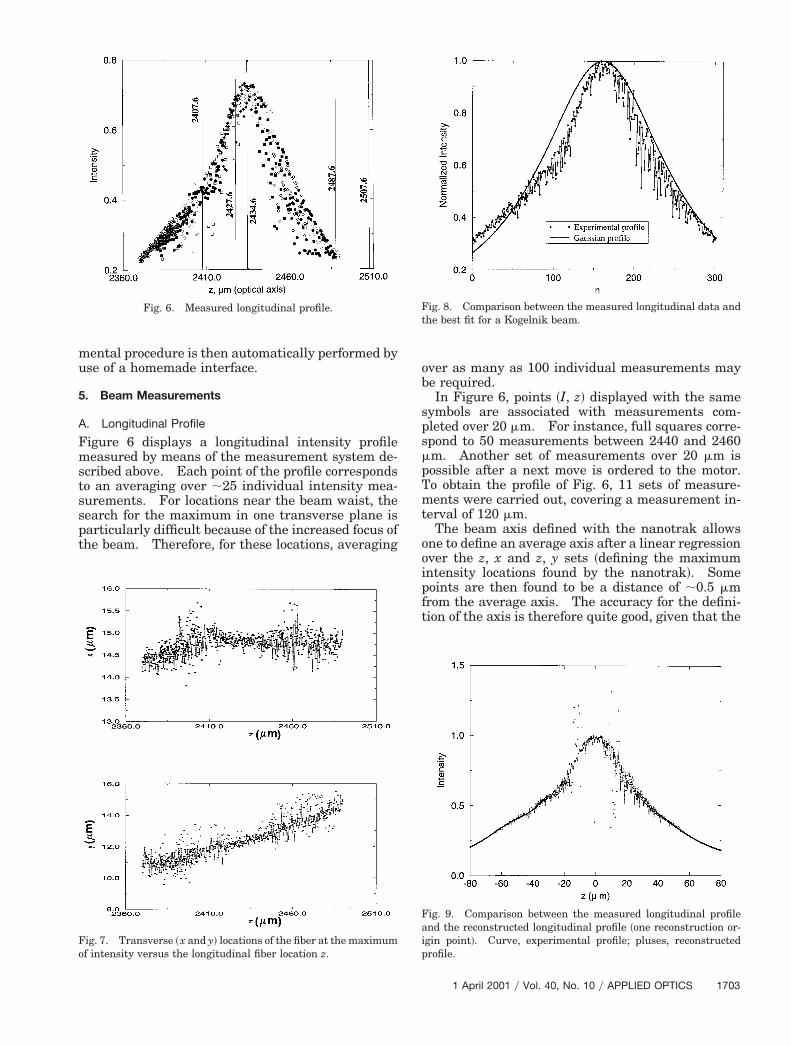
Figure 6 displays a longitudinal intensity profilemeasured by means of the measurement system de-scribed above. Each point of the profile correspondsto an averaging over ;25 individual intensity mea-surements. For locations near the beam waist, thesearch for the maximum in one transverse plane isparticularly difficult because of the increased focus ofthe beam. Therefore, for these locations, averaging

Fig. 6. Measured longitudinal profile.

Fig. 7. Transverse ~x and y! locations of the fiber at the maximumf intensity versus the longitudinal fiber location z.

over as many as 100 individual measurements maybe required.

In Figure 6, points ~I, z! displayed with the samesymbols are associated with measurements com-pleted over 20 mm. For instance, full squares corre-spond to 50 measurements between 2440 and 2460mm. Another set of measurements over 20 mm is

ossible after a next move is ordered to the motor.o obtain the profile of Fig. 6, 11 sets of measure-ents were carried out, covering a measurement in-

erval of 120 mm.The beam axis defined with the nanotrak allows

ne to define an average axis after a linear regressionver the z, x and z, y sets ~defining the maximumntensity locations found by the nanotrak!. Someoints are then found to be a distance of ;0.5 mmrom the average axis. The accuracy for the defini-ion of the axis is therefore quite good, given that the

Fig. 8. Comparison between the measured longitudinal data andthe best fit for a Kogelnik beam.

Fig. 9. Comparison between the measured longitudinal profileand the reconstructed longitudinal profile ~one reconstruction or-igin point!. Curve, experimental profile; pluses, reconstructedprofile.


t

nafitmatdpTtIw

bb

m

pr

i1am

1

intensity measurements are carried out with a 3-mmip ~see Fig. 7!.

The profile presented in Fig. 6 is a rough one; i.e.,o point has been rejected. However, some pointsre erroneous when, sometimes, the nanotrak fails tond a maximum. To reject these points, we rely onhe standard deviation of the intensity measure-ents. Each intensity measurement is actually an

verage and, in the case of a poorly determined point,he standard deviation over the data is large. Aftereleting these points, we obtain the profile that islotted in Fig. 8 with the label “Experimental profile.”his final profile is made from 300 points, the dis-

ance between two successive points being 0.4 mm.ntensities have been normalized such that, at beam-aist location, the normalized intensity is unity.In Fig. 8 a profile corresponding to a Gaussian

eam ~as defined by Kogelnik! is also plotted. Theeam-waist radius v0 ~equal to 2.7 mm! was deter-

mined from a best fit with experimental data. Thisfigure indicates that the experimental profile signif-icantly departs from a theoretical Gaussian beam.In particular, we can note that the experimental pro-file is not symmetrical. In such a case the interest ofthe determination of actual BSC’s is warranted.

To run the nonlinear inversion technique, we needinitial guess values for the special BSC’s gn. Start-ing from these guess values, the inversion techniquerelies on a singular-value-decomposition algorithmthat requires approximately three loops. The guessBSC’s that are used to initialize the process are cho-sen in a realistic way; namely, they are coefficients ofthe Gaussian ~Kogelnik! profile in Fig. 8.

The result of the inversion technique generates aset of coefficients gn. Using these coefficients, de-duced from experimental measurements, we can plota new longitudinal profile of intensity, which we callthe reconstructed profile. The two profiles ~experi-

ental profile and reconstructed profile! are com-

Fig. 10. Comparison between the measured longitudinal profileand the reconstructed longitudinal profile ~eight reconstructionorigin points!. Circles, measured; dotted curve, reconstructed;dashed curve, Gaussian.


ared in Fig. 9, exhibiting three different kinds ofegion:

• In region 1, close to the beam-waist center, thereconstruction is close to the experiments, includingat the scale of the small fluctuations. For this re-construction the center of the partial wave expansionwas chosen at the beam waist. In fact, the recon-struction is satisfactory around the partial wave ex-pansion center. For the case under study this regionextends over 68 mm around this center.

• Farther away from the center, in a region la-beled 2, we can see that the reconstruction is stillsatisfactory, except for some points that are outliers,departing appreciably from the mean curve. For ex-ample, at location z 5 9.9967 mm, the reconstructedntensity is dramatically large, namely, larger than.25. The set of such points has no physical sensend is actually due to numerical instabilities. Itust be noted, however, that these numerical insta-

Fig. 11. Comparison between extracted BSC’s and filtered BSC’s:~a! Real part versus n. ~b! Imaginary part versus n. Gray curve,reconstructed; dotted–dashed curve, measured.

eccr

wI

e

c

tici

bilities occur only for points that do not coincide withmeasurement points in the measurement interval.Conversely, we observe quite good agreement be-tween experiments and reconstructions for pointscorresponding to measurement points.

• In the final region, labeled 3, that is to say, farfrom the wave expansion center, there is, as a whole,good agreement between the measured profile andthe reconstructed profile, but the reconstructed pro-file smooths the small-scale fluctuations. Therefore,in this region, the inversion process acts as a noise-filtering process. This region extends out far fromthe measurement domain.

If another point is chosen as a center for the partialspherical wave expansion, then the above resultswith three regions is still valid. In any case, the

Fig. 12. Comparison between the measured longitudinal profileand the reconstructed longitudinal profile for one reconstructionorigin point but with filtered BSC’s.

Fig. 13. Comparison between the measu

global behavior of the profile is still recovered. Toeliminate the main drawback of the present inversionprocess ~large departures in region 2!, we now pro-pose two different solutions.

The first solution consists of using more than onepartial wave expansion center. Indeed, in region 1~that is to say, actually around the center of inversiondomain!, the intensity profile is well predicted, lead-ing to the idea of concatenating the result of severalregions 1 for different origins of the partial waveexpansions. The result is plotted in Fig. 10. Sinceregion 1 is ;16 mm wide whatever the origin forxpansions is, eight regions labeled 1 have been con-atenated to recover the totality of the profile. Wean observe that there is no outlier on this piecewiseeconstructed profile.

The second solution consists of filtering the BSC’sith only one point for the partial wave expansion.

n Fig. 11, coefficients gn resulting from the inversionprocess have been plotted. Figures 11~a! and 11~b!xhibit Re~gn! and Im~gn!, respectively. The center

for the partial spherical wave expansion was chosenat the beam focus. The inversion over 300 points~Fig. 8! therefore can provide us with as many as 150oefficients gn. However, the number of coefficients

gn required for calculating the Gaussian beam profileof Fig. 8 is equal to ;100. Consequently, the sum-mation in relation ~1! can be in practice numericallyruncated at n . 100 for the case under study. Thiss why the inversion was carried out for 100 or 110oefficients as displayed in Fig. 11. From this figuret is observed that the coefficients gn exhibit an oscil-

latory character, particularly for high values of n.We then remove high-frequency oscillations bymeans of a Fourier filter. The coefficients gn thenobtained are plotted in bold curves in Fig. 11. Usingthe filtered coefficients of Fig. 11, we calculate thelongitudinal intensity profile plotted in Fig. 12. We

ap and the reconstructed intensity map.
red m

fiotvwt

t

aNc

1

observe that the shape of the measured profile issatisfactorily predicted. Also, as a result of the high-frequency filtering, the reconstructed profile issmooth. Let us recall that this satisfactory result isobtained here by use of a single partial wave expan-sion, with origin at the beam-waist center.

B. Transverse Profile

The knowledge of measured BSC’s is equivalent to theknowledge of electromagnetic fields everywhere inspace and, therefore, should allow one, in particular, toalso recover transverse profiles of intensity. Indeed,let us consider Fig. 13. In Fig. 13~a! an experimentaltransverse map of intensity is plotted. To obtain it,the optical fiber fastly scans the beam, line by line.During this process some misalignments between linesmay occur, giving the map a fairly fuzzy character.The resolution between two points is equal to 100 nm.Figure 13~b! displays the corresponding reconstructedintensity map, obtained by use of the BSC’s of Fig. 11.The reconstructed map exhibits a rotational symmetrybecause special BSC’s are used. The comparison be-tween the measured and the reconstructed maps isthen satisfactory.

6. Conclusion

We have experimentally demonstrated the possibilityof determining special beam-shape coefficients~BSC’s! gn of an actual beam in the laboratory, both inamplitude and phase, from intensity measurementsalong the beam axis. These experimental coeffi-cients can be used as an input to the generalizedLorenz–Mie theory ~GLMT! and could allow for re-

ned particle characterization or a better masteringf radiation pressure forces for the design of opticalweezers. The formulation for a similar study, de-oted to BSC’s gn

m is ready ~Ref. 7! and, very likely,ould be amenable to experimental tests, extending

he results presented in this paper.

J. Heline carried out the computations concerninghe effect of a finite-size detector ~Section 3!, and we


lso acknowledge the financial support of the Haute-ormandie district, France, for the experimental fa-

ilities.

References1. G. Gouesbet and G. Grehan, “Generalized Lorenz–Mie theo-

ries, from past to future,” Atomization Sprays 10, 277–333~2000!.

2. K. F. Ren, G. Gouesbet, and G. Grehan, “Integral localizedapproximation in generalized Lorenz–Mie theory,” Appl. Opt.37, 4218–4225 ~1998!.

3. K. F. Ren, G. Grehan, and G. Gouesbet, “Prediction of reverseradiation pressure by generalized Lorenz–Mie theory,” Appl.Opt. 35, 2702–2710 ~1996!.

4. J. T. Hodges, G. Grehan, G. Gouesbet, and C. Presser, “For-ward scattering of a Gaussian beam by a nonabsorbingsphere,” Appl. Opt. 34, 2120–2132 ~1995!.

5. J. A. Lock and J. T. Hodges, “Far-field scattering of an axisym-metric laser beam of arbitrary profile by an on-axis sphericalparticle,” Appl. Opt. 35, 4283–4290 ~1996!.

6. J. A. Lock and J. T. Hodges, “Far-field scattering of non-Gaussian off-axis axisymmetric laser beam by a spherical par-ticle,” Appl. Opt. 35, 6605–6616 ~1996!.

7. G. Gouesbet, “On measurements of beam shape coefficients ingeneralized Lorenz–Mie theory and the density-matrix ap-proach. I. Measurements,” Part. Part. Syst. Charact. 14,12–20 ~1997!.

8. G. Gouesbet, “On measurements of beam shape coefficients ingeneralized Lorenz–Mie theory and the density-matrix ap-proach. II. The density-matrix approach,” Part. Part. Syst.Charact. 14, 88–92 ~1997!.

9. H. Polaert, G. Gouesbet, and G. Grehan, “Measurement ofbeam-shape coefficients in the generalized Lorenz–Mie theoryfor the on-axis case,” Appl. Opt. 37, 5005–5013 ~1998!.

10. L. W. Davis, “Theory of electromagnetic beams,” Phys. Rev. A19, 1177–1179 ~1979!.

11. G. Gouesbet, G. Grehan, and B. Maheu, “Computations ofthe coefficients gn in the generalized Lorenz–Mie theory us-ing three different methods,” Appl. Opt. 27, 4874–4883~1988!.

12. G. Gouesbet, “Validity of the localized approximation for arbi-trary shaped beams in generalized Lorenz–Mie theory forspheres,” J. Opt. Soc. Am. A 16, 1641–1650 ~1999!.

Date post:	30-Sep-2016
Category:	Documents
Upload:	gerard
View:	214 times
Download:	2 times

Laboratory Determination of Beam-Shape Coefficients for Use in Generalized Lorenz-Mie Theory

Documents