167
EPA-600-R-16-357 Laboratory, Field, and Analytical Procedures for Using Passive Sampling in the Evaluation of Contaminated Sediments: User’s Manual February 2017 Final Web Version (1.0)
EPA-600-R-16-357
Laboratory, Field, and Analytical Procedures for Using Passive Sampling in the Evaluation of Contaminated Sediments: User’s Manual
February 2017 Final Web Version (1.0)

Laboratory, Field, and Analytical Procedures for Using Passive
Sampling in the Evaluation of Contaminated Sediments:
User’s Manual
Robert M. Burgess
U.S. Environmental Protection Agency
National Health and Environmental Effects Research Laboratory
Atlantic Ecology Division, Narragansett, RI, USA
Susan B. Kane Driscoll
Exponent, Inc.
Maynard, MA, USA
G. Allen Burton
Cooperative Institute for Limnology & Ecosystems Research
University of Michigan Water Center
Ann Arbor, MI, USA
Upal Ghosh
Department of Chemical, Biochemical, & Environmental Engineering
University of Maryland Baltimore County
Baltimore, MD, USA
Philip M. Gschwend
Parsons Laboratory for Environmental Science and Engineering
Massachusetts Institute of Technology
Cambridge, MA, USA
Danny Reible
Department of Civil and Environmental Engineering
Texas Tech University
Lubbock, TX, USA
Sungwoo Ahn
Exponent, Inc.
Bellevue, WA, USA
Tim Thompson
Science and Engineering for the Environment, LLC
Seattle, WA 98105
U.S. Environmental Protection Agency
Office of Research and Development
National Health and Environmental Effects Research Laboratory
Atlantic Ecology Division, Narragansett, RI 02882
Strategic Environmental Research and Development Program (SERDP)/
Environmental Security Technology Certification Program (ESTCP)
4800 Mark Center Dr.
Alexandria, VA 22350

PASSIVE SAMPLING: USER’S MANUAL
ii
Notice
The Department of Defense’s Strategic Environmental Research and Development Program
(SERDP)/Environmental Security Technology Certification Program (ESTCP) and U.S. EPA’s Office
of Research and Development (ORD) produced this document as a guide for using passive sampling to
evaluate contaminated sediments. The document is intended to cover the laboratory, field, and
analytical aspects of passive sampler applications. This document will be useful for developing user-
specific laboratory, field and analytical procedures and as a complement to existing sediment
assessment tools. This document should be cited as:
U.S. EPA/SERDP/ESTCP. 2017. Laboratory, Field, and Analytical Procedures for Using
Passive Sampling in the Evaluation of Contaminated Sediments: User’s Manual. EPA/600/R- 16/357. Office of Research and Development, Washington, DC 20460
Most information in this document has been funded wholly by the DOD’s Strategic Environmental
Research and Development Program/Environmental Security Technology Certification Program with
some content provided by the U.S. Environmental Protection Agency. This document has been
subjected to Agency peer and administrative review and has been approved for publication as an EPA
document.
Mention of trade names or commercial products does not constitute endorsement or
recommendation for use. This document is U.S. EPA Science Inventory #308731.
For optimum readability, print and view this document in color. Further, when printing the
document pdf, make sure that sufficient dots per inch (dpi) are used to attain acceptable resolution
(e.g., 300-400 dpm).
EXECUTIVE SUMMARY
iii
Executive Summary
Addressing the human and ecological health risks associated with contaminated sediments
represents one of the most wide-spread and technically challenging environmental problems. In the
United States, monitoring programs coordinated by the U.S. Environmental Protection Agency (U.S.
EPA), National Oceanic and Atmospheric Administration (NOAA) and other organizations have
documented that vast quantities of freshwater and marine sediments are moderately to severely
contaminated with chemical pollutants (Daskalakis and O’Connor 1995, U.S. EPA 1996a, b, 1997a,b,c,
1998, 2004). Further, several other countries around the world also wrestle with related contaminated
sediments issues (e.g., Australia, New Zealand, the Netherlands, China, the United Kingdom [Babut et
al. 2005, Chen et al. 2006]). Based on surveys performed in the United States, the quantities of
contaminated sediments present in the environment approach billions of metric tons. To reduce or
eliminate the human and ecological health risks manifested by these sediments, federal, state, local, and
tribal regulatory authorities have a range of remedial technologies available including dredging, various
forms of capping, and natural monitored recovery (NMR) (U.S. EPA 2005a). Each technology has
advantages and disadvantages including effectiveness and costs. For example, the on-going remediation
of the Hudson River Superfund site involves the removal, via dredging, of over two million metric tons
of contaminated sediments at a potential cost of over a billion dollars
(http://www.epa.gov/superfund/accomp/success/hudson.htm). Estimated costs associated with
managing all contaminated sediments in terms of remediation and post-operational monitoring are in the
tens of billions of U.S. dollars (U.S. EPA 2005a).
Regardless of the remedial technology invoked to address contaminated sediments in the
environment, there is a critical need to have tools for designing and assessing the effectiveness of the
remedy. In the past, these tools have included chemical and biomonitoring of the water column and
sediments, toxicity testing and bioaccumulation studies performed on site sediments, and application of
partitioning, transport and fate modeling. All of these tools served as lines of evidence for making
informed environmental management decisions at contaminated sediment sites. In the last ten years, a
new tool for assessing remedial effectiveness has gained a great deal of attention. Passive sampling
offers a tool capable of measuring the freely dissolved concentrations (Cfree) of legacy contaminants in
water and sediments. In addition to assessing the effectiveness of the remedy, passive sampling can be
applied for a variety of other contaminated sediments site purposes involved with performing the
preliminary assessment and site inspection, conducting the remedial investigation and feasibility study,
preparing the remedial design, and assessing the potential for contaminant bioaccumulation (U.S. EPA
2005a).
While there is a distinct need for using passive sampling at contaminated sediments sites and several
previous documents and research articles have discussed various aspects of passive sampling (e.g.,
Vrana et al. 2005, Lohmann 2012, Reible and Lotufo 2012, Smedes and Booij 2012, U.S. EPA 2012a, b,
Ghosh et al. 2014, Mayer et al. 2014, Peijnenburg et al. 2014), there has not been definitive guidance on
the laboratory, field and analytical procedures for using passive sampling at contaminated sediment
sites. This document is intended to provide users of passive sampling with the guidance necessary to
apply the technology to evaluate contaminated sediments. The contaminants discussed in the document
include primarily polychlorinated biphenyls (PCBs), polycyclic aromatic hydrocarbons (PAHs), and the
metals, cadmium, copper, nickel, lead and zinc. Other contaminants including chlorinated pesticides

PASSIVE SAMPLING: USER’S MANUAL
iv
and dioxins and furans are also discussed. The document is divided into ten sections each discussing
aspects of passive sampling including the different types of samplers used most commonly in the United
States, the selection and use of performance reference compounds (PRCs), the extraction and
instrumental analysis of passive samplers, data analysis and quality assurance/quality control, and an
extensive list of passive sampling related references. In addition, the document has a set of appendices
which discuss facets of passive sampling in greater detail than possible in the main document. More
specifically, included in the appendices are two examples of quality assurance project plans (QAPPs).
This information is intended to provide a sound foundation for passive sampler users to apply this
technology. This document does not, however, cover the critical planning process that would be used to
arrive at the need for passive sampling. Additional information on the planning process can be found in
the guidance document, Integrating Passive Sampling Methods into Management of Contaminated
Sediment Sites (ESTCP 2016).
This document is not intended to serve as a series of standard operating procedures (SOPs) for using
passive samplers at contaminated sediment sites. Rather, the document seeks to provide users with the
information needed to develop their own SOPs or similar procedures. To this end, along with the
information provided in the document, the names of selected passive sampling experts are listed who
can be contacted to answer specific questions about the laboratory, field and analytical procedures
associated with passive sampling. Additional information on passive samplers (including this document), SOPs and case studies can also be found on the ESTCP and U.S. EPA Superfund websites:
https://www.serdp-estcp.org/Featured-Initiatives/Cleanup-Initiatives/Bioavailability
https://www.epa.gov/superfund/superfund-contaminated-sediments-guidance-document-fact-sheets-
and-policies
CONTENTS
v
Contents
Introduction .................................................................................................................................. 1 Objectives of User’s Manual ....................................................................................................... 1
Background .................................................................................................................................. 1 Types of Passive Samplers and Deployments ............................................................................. 4 Principles of the Passive Sampling of Target Hydrophobic Organic Contaminants ................... 9 Principles of the Passive Sampling of Metals ............................................................................ 11 Applications ............................................................................................................................... 13
Hydrophobic Organic Contaminants ............................................................................... 13
Metals .............................................................................................................................. 14
Additional Passive Sampler Needs and Current Resources ....................................................... 15 Commercial Laboratory Considerations .................................................................................... 16
Use of Project Teams ...................................................................................................... 16 Role of this Document’s Methods ................................................................................... 17
Defining “Immediately” in this Document ..................................................................... 17 Availability of Passive Sampler Partition Coefficients ................................................... 17
Document Overview .................................................................................................................. 23 Passive Sampling with Polyoxymethylene (POM) .................................................................... 24 Introduction ................................................................................................................................ 24
Laboratory Preparation .............................................................................................................. 24
POM Selection and Pre-Cleaning .................................................................................... 25 Selection of POM:Sediment Ratio .................................................................................. 25 Selection of Sediment Mass to be used for Cfree Determinations .................................... 26
Exposure Time and Conditions ....................................................................................... 26 Use of Biocides to Inhibit Target Contaminant Biodegradation ..................................... 26
Field Use .................................................................................................................................... 27 In situ Deployment Device Designs ................................................................................ 27
Recovery and Processing ........................................................................................................... 27
Extraction and Instrumental Analysis ........................................................................................ 29 Data Analysis ............................................................................................................................. 29
Selection of Published POM-Water Partition Coefficients (KPOM) ........................................... 29
Empirical Determination of KPOM Partition Coefficients .......................................................... 29 Passive Sampling with Polydimethylsiloxane (PDMS) ............................................................. 31 Introduction ................................................................................................................................ 31
Laboratory Preparation .............................................................................................................. 34 Pre-cleaning and Ex situ Deployment ............................................................................. 34
Field Use .................................................................................................................................... 34 Pre-deployment Preparation ............................................................................................ 34 In situ Deployment .......................................................................................................... 35
Recovery and Processing ........................................................................................................... 36 Extraction and Instrumental Analysis ........................................................................................ 37 Data Analysis ............................................................................................................................. 37
Selection of Published PDMS-Water Partition Coefficients (KPDMS) ....................................... 37 Passive Sampling with Low-Density Polyethylene (LDPE) ...................................................... 39 Introduction ................................................................................................................................ 39

PASSIVE SAMPLING: USER’S MANUAL
vi
Laboratory Use........................................................................................................................... 39 Pre-Deployment Preparation ........................................................................................... 39 Ex situ Deployment ......................................................................................................... 40
Field Use .................................................................................................................................... 40
Recovery and Processing ........................................................................................................... 42 Extraction and Instrumental Analysis ........................................................................................ 44 Data Analysis ............................................................................................................................. 44 Selection of Published Low-Density Polyethylene-WaterPartition Coefficients (KLDPE) ......... 44 Passive Sampling with Diffusive Gradient in Thin Films (DGT) .............................................. 45
Introduction ................................................................................................................................ 45 Preparation and Laboratory Use ................................................................................................ 47
Field Use .................................................................................................................................... 47 Recovery and Processing ........................................................................................................... 48 Extraction and Instrumental Analysis ........................................................................................ 48 Data Analysis ............................................................................................................................. 48
Selection and Use of Performance Reference Compounds for Hydrophobic
Organic Target Contaminants ....................................................................................................... 49
Introduction ................................................................................................................................ 49 Using Performance Reference Compounds (PRCs) .................................................................. 49
Selecting PRCs ................................................................................................................ 49
Loading PRCs .................................................................................................................. 50 Determining the Quantity of PRC to Load into Passive Samplers .................................. 53
Example Calculation ....................................................................................................... 54 Chemical Analysis of PRCs following Deployment ....................................................... 55
Extraction and Instrumental Analysis of Target Contaminants from Passive Sampling ........... 56 Introduction ................................................................................................................................ 56
Extraction for POM, PDMS, and LDPE .................................................................................... 60 7.2.1 Extraction of POM .......................................................................................................... 60 7.2.2 Extraction of PDMS ........................................................................................................ 60
7.2.3 Extraction of LDPE ......................................................................................................... 63 Instrumental Chemical Analysis for POM, PDMS and LDPE .................................................. 65
Instrumental Detection Limits for POM, PDMS and LDPE ........................................... 65 Extraction of DGT ..................................................................................................................... 69
Instrumental Chemical Analysis of DGT .................................................................................. 69 7.5.1 Instrumental Detection Limits for DGT .......................................................................... 69
Data Analysis: Calculation of Cfree and CDGT ............................................................................. 70 Introduction ................................................................................................................................ 70 POM, PDMS, and LDPE Data Analysis .................................................................................... 71
Equilibrium Conditions ................................................................................................... 72 Non-Equilibrium Conditions using PRCs ....................................................................... 72
Example Calculations: Equilibrium versus Non-Equilibrium Conditions ...................... 75 DGT Data Analyses ................................................................................................................... 83
Example DGT Calculations ............................................................................................. 83 Case Studies ............................................................................................................................... 83
Quality Assurance and Quality Control, and Other Considerations .......................................... 84 Introduction ................................................................................................................................ 84

CONTENTS
vii
Hydrophobic Organic Contaminant Polymer-Specific Quality Assurance
and Quality Control.................................................................................................................... 85 Polymer-Specific Deployment Blanks (i.e., trip blanks, field blanks) ............................ 85 Field Solvent Blanks ....................................................................................................... 85
Field Control Samples ..................................................................................................... 85 Field Internal Standards ................................................................................................... 86 Recoveries of Surrogate Standards (also known as Internal Standards) ......................... 86 PRC-Loaded Passive Sampler Reproducibility ............................................................... 86 QC Samples for Chemical Analysis ................................................................................ 86
Specific Quality Assurance for POM .............................................................................. 86 Specific Quality Assurance for PDMS ............................................................................ 87
Specific Quality Assurance for LDPE ............................................................................. 87 Passive Sampling Example Sampling and Analysis Project Plan (SAP)
and Quality Assurance Project Plan (QAPP) .................................................................. 88 DGT-Specific Quality Assurance and Quality Control ............................................................. 88
DGT Quality Control ....................................................................................................... 88 DGT Quality Assurance .................................................................................................. 88
References .............................................................................................................................. 90
Appendix A: Provisional Passive Sampler Partition Coefficients (KPS) for PCBs and PAHs .........103
Appendix B: Additional Passive Sampler Partition Coefficient Information ..................................107
Appendix C: Effects of Temperature and Salinity on Polymer-Water Partition Coefficients .........115
Appendix D: Diffusion Coefficients (D) for Metals used in DGTs .................................................117
Appendix E: Quality Guidelines for Hydrophobic Organic Contaminant Analysis ........................118
Appendix F: Case Studies.................................................................................................................127
Appendix G: Example Quality Assurance Project Plan (QAPP) .....................................................153
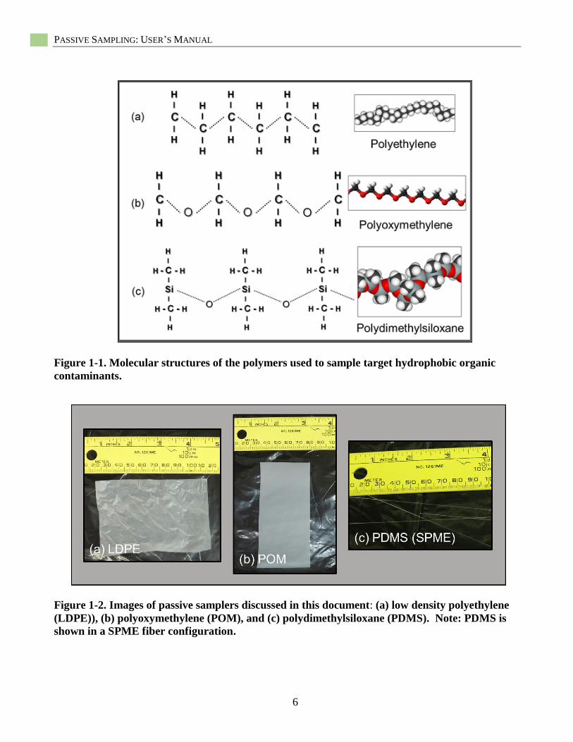
Figures Figure 1-1. Molecular structures of the polymers used to sample target hydrophobic organic
contaminants. ........................................................................................................................................ 6
Figure 1-2. Images of passive samplers discussed in this document .......................................................... 6
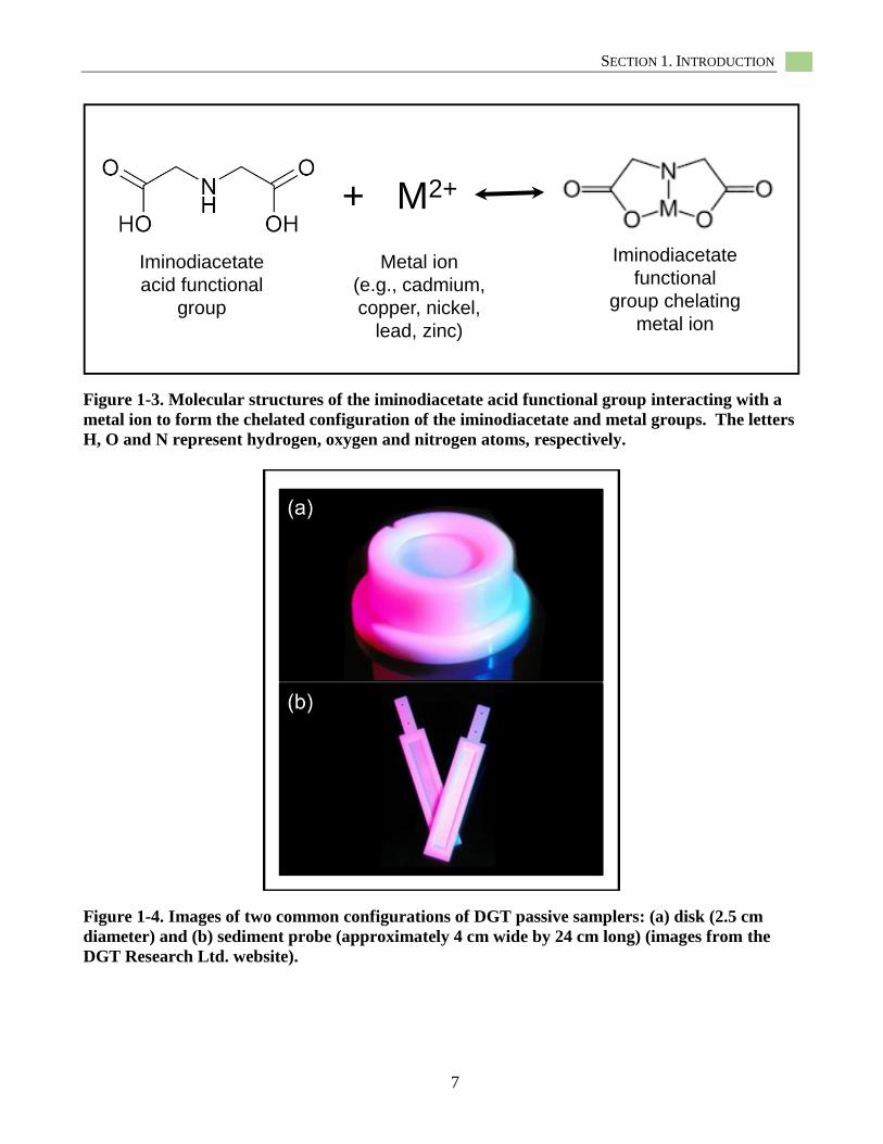
Figure 1-3. Molecular structures of the iminodiacetate acid functional group ........................................... 7
Figure 1-4. Images of two common configurations of DGT passive samplers .......................................... 7
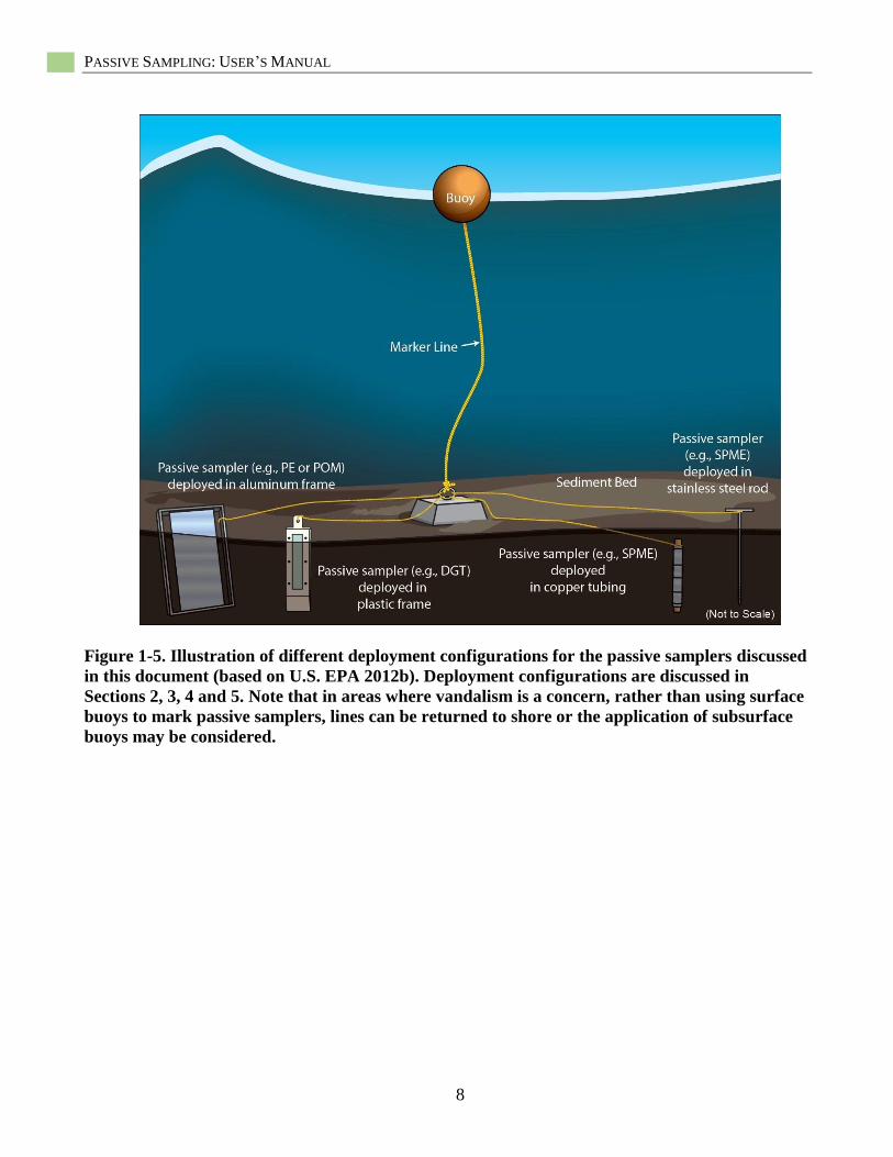
Figure 1-5. Illustration of different deployment configurations for the passive samplers.......................... 8
Figure 1-6. Cartoon showing the three stages of passive sampler operation ............................................ 10
Figure 2-1. Polyoxymethylene passive sampler strip in a laboratory vial ................................................ 28
Figure 2-2. Polyoxymethylene passive sampler strips .............................................................................. 28
Figure 3-1. Schematic of solid phase microextraction fiber showing the outer coating
of polydimethylsiloxane...................................................................................................................... 32
Figure 3-2. Insertion of a PDMS coated SPME fiber into whole sediments ............................................ 32
PASSIVE SAMPLING: USER’S MANUAL
viii
Figure 3-3. Shielded and unshielded holders forPDMS coated SPME fibers with insets ........................ 33
Figure 3-4. SPME fibers configured to be wrapped in fine stainless steel mesh ...................................... 33
Figure 4-1. Sequence of steps used to prepare passive samplers for in situ field deployment ................. 40
Figure 4-2. Schematic of a LDPE passive sampling configuration using two aluminum sheet frames ... 41
Figure 4-3. LDPE film deployed inside an aluminum mesh packet. ........................................................ 42
Figure 4-4. Photographs of various systems for deploying LDPE in the water column .......................... 43
Figure 4-5. Photograph of LDPE in an aluminum frame after deployment ............................................. 43
Figure 5-1. Schematic of commercial DGT disks in (a) cross-section and (b) DGT sediment probes
in exploded view ................................................................................................................................. 46
Figure 5-2. Theoretical diagram of metal concentrations in the DGT device .......................................... 46
Figure 5-3. Photograph of the ex situ deployment of DGT samplers in simulated water column............ 47
Figure 6-1. Sequence of steps used to prepare passive samplers for field deployment ............................ 52
Figure 7-1. Illustration of basic steps involved in preparing an in situ deployed passive sampler .......... 58
Figure 8-1. Flow chart of the approaches for analyzing passive sampler data ......................................... 73
Figure 8-2. Flow chart for selecting the appropriate PRC Correction Calculator .................................... 74
Figure 8-3. Primary data entry points and basic layout of the graphical user interface ........................... 76
Figure 8-4. Example output from the GUI for the PDMS PRC Correction Calculator ............................ 77
Figure 8-5. Primary data entry points and basic layout of the GUI .......................................................... 78
Figure 8-6. Example output from the GUI for the sediment deployment LDPE PRC
Correction Calculator .......................................................................................................................... 79
Figure 8-7. Primary data entry points and basic layout of the GUI .......................................................... 80
Figure 8-8. Example of data entry window (‘UserForm1’) ...................................................................... 80
Figure 8-9. Example output from the GUI for the water column deployment ......................................... 81
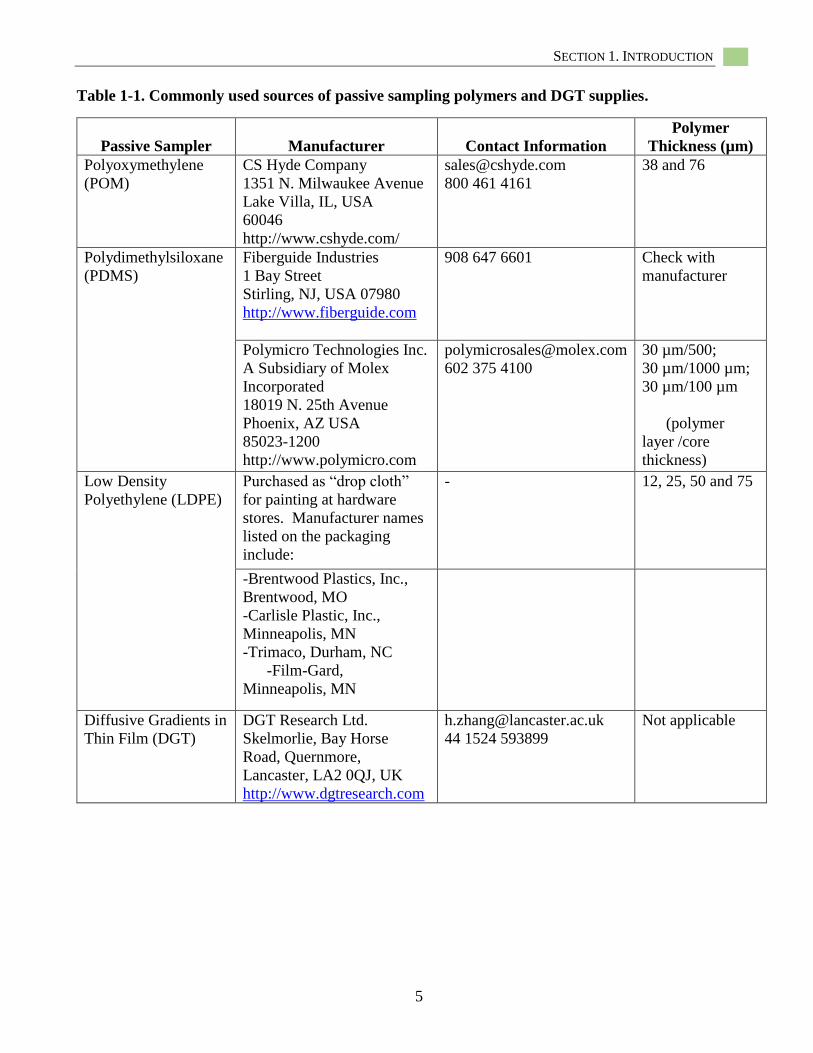
Tables Table 1-1. Commonly used sources of passive sampling polymers and DGT supplies. ............................ 5
Table 1-2. Application of passive samplers at selected U.S. EPA Superfund sites .................................. 18
Table 1-3. Advantages and disadvantages of different types of passive samplers ................................... 19
Table 1-4. List of academic and governmental technical contacts ........................................................... 20
Table 1-5. Examples of commercial analytical laboratories ..................................................................... 22
Table 1-6. Additional costs for commercial laboratories .......................................................................... 23
Table 6-1. Examplea performance reference compounds (PRCs) ............................................................ 53
Table 7-1. Summary of extraction and analytical methods for passive samplers ..................................... 59
Table 7-2. Representative target contaminant detection limitsa for POM. ............................................... 67
Table 7-3. Representative target contaminant detection limits for PDMS. .............................................. 68
Table 7-4. Representative target contaminant detection limits for LDPE. ............................................... 69
Table 8-1. Example calculations of Cfree for 11 PCB congeners and total PCBs ..................................... 82
Table 9-1. Summary of quality assurance and quality control samples ................................................... 84

ACKNOWLEDGEMENTS
ix
Acknowledgements Scientific Contributions
Steve Ells U.S. EPA, Office of Land and Emergency Management,
Washington, DC, USA
Loretta Fernandez Northeastern University, Boston, MA, USA
Abbey Joyce National Research Council, U.S. EPA, Office of Research and
Development, Narragansett, RI, USA
Matthew Lambert U.S. EPA, Office of Land and Emergency Management,
Washington, DC, USA
Keith Maruya Southern California Coastal Water Research Project Authority,
Costa Mesa, CA, USA
Monique Perron U.S. EPA, Office of Chemical Safety and Pollution Prevention,
Office of Pesticides, Washington, DC, USA
Ariette Schierz Exponent, Inc., Maynard, MA, USA
Technical Reviewers Mark Cantwell U.S. EPA, Office of Research and Development, Narragansett, RI, USA
Loretta Fernandez Northeastern University, Boston, MA, USA
Sandra Fogg U.S. EPA, Office of Research and Development, Narragansett, RI, USA
Kay Ho U.S. EPA, Office of Research and Development, Narragansett, RI, USA
Alan Humphrey U.S. EPA, Region 2, Edison, NJ, USA
Abigail Joyce National Research Council, U.S. EPA, Office of Research and
Development, Narragansett, RI, USA
Matthew Lambert U.S. EPA, Office of Land and Emergency Management,
Washington, DC, USA
Joseph LiVolsi U.S. EPA, Office of Research and Development, Narragansett, RI,
USA
Patricia McIssac Test America, Oakton, VA, USA
Thomas Parkerton ExxonMobil Biomedical Sciences Inc. Spring, Texas, USA
Kathleen Schweitzer United States Coast Guard, Warwick, RI, USA
Sean Sheldrake U.S. EPA, Region 10, Seattle, WA, USA
Patricia DeCastro CSRA, International, Narragansett, RI, USA

PASSIVE SAMPLING: USER’S MANUAL
x
Acronyms
A surface area of DGT exposed to sediment
AVS acid volatile sulfides
BLM biotic ligand model
CB chlorinated biphenyl
CCV continuing calibration verification 13C12 Carbon13 labelled form a compound
CDGT diffusion gradient in thin film concentration
Ce metal concentration in acid extract
Cfree freely dissolved concentration
CITW interstitial water or porewater concentration
CLDPE low density polyethylene concentration
CPDMS polydimethylsiloxane concentration
CPolymer DL detection limit for the passive sampler concentration
CPOM polyoxymethylene concentration
CPRCi performance reference compound initial concentration
CPRCf performance reference compound final concentration
CPS passive sampler concentration
CPSnon-eq non-equilibrium passive sampler concentration
CSed target contaminant sediment concentration
Cw water concentration
CW DL method detection limit of water using a given passive sampler
COD coefficient of determination
D diffusion coefficient of the resin gel
Dx Deuterated labelled form of a compound
DDD dichlorodiphenyldichloroethane
DDE dichlorodiphenyldichloroethylene
DDT dichlorodiphenyltrichloroethane
DGT diffusive gradient in thin films
DI deionized water
DOC dissolved organic carbon
DOD Department of Defense
EICP extracted ion current profile
EPA U.S. Environmental Protection Agency
EqP equilibrium partitioning
fe elution factor
feq fraction equilibrium
fmeq PRCx measured fractional equilibrium for PRC
GC gas chromatography
GC/ECD gas chromatography/electron capture detection
GC/ELCD gas chromatography/electrolytic conductivity detector
GC/MS gas chromatography/mass spectrometry
GC/FID gas chromatography/flame ionization detector
GUI graphical user interface
HOC hydrophobic organic chemical
HPLC high-performance liquid chromatography

ACRONYMS
xi
HRGC high-resolution gas chromatography
HRMS high-resolution mass spectrometry
ICAL initial calibration for all analytes
ICP-MS inductively coupled plasma mass spectrometry
ICP-OES inductively coupled plasma optical emission spectrometry
ICV initial calibration verification
ke exchange rate constant for the target contaminant
KD sediment-water partition coefficient
Kf SPME fiber-water portioning coefficient (approximately equivalent to KPDMS)
KLDPE low-density polyethylene-water partitioning coefficient
KOW octanol-water partitioning coefficient
KPDMS polydimethylsiloxane-water partitioning coefficient
KPOM polyoxymethylene-water partition coefficient
KPS passive sampler-water partition coefficient
KS Setschenow constant
LCS laboratory control sample
LDPE low-density polyethylene
LFER linear free energy relationship
LRMS low-resolution mass spectrometry
M mass of metal in resin gel
MDL method detection limit
MGP manufactured gas plant
MRL method reporting limit
MS mass spectrometry
n sample size
nDetection mass of contaminant detected
NAPL non-aqueous phase liquid
NOAA National Oceanic and Atmospheric Administration
NMR Natural monitored recovery
PAH polycyclic aromatic hydrocarbon
PCB polychlorinated biphenyl
PCC PRC correction calculator
PCDD polychlorinated dioxin
PCDF polychlorinated diphenyl furan
PDMS polydimethylsiloxane
PE polyethylene
PED polyethylene device
POM polyoxymethylene
PPE personal protective equipment
PQL practical quantitation limit
PRC performance reference compound
PS passive sampler or passive sampling
PSD passive sampling device
PSM passive sampling method
QA-QC quality assurance, quality control
R gas constant (8.31 J/mol K)
RDGT ratio of CDGT to CITW
RRT relative retention time
PASSIVE SAMPLING: USER’S MANUAL
xii
RSD relative standard deviation
[salt] salt concentration
SD standard deviation
SE standard error
SEM simultaneously extracted metals
SETAC Society of Environmental Toxicology and Chemistry
SOP Standard operating procedures
SPMD semi-permeable membrane device
SPME solid-phase micro-extraction
SS stainless steel
SVOC semi-volatile organic compound
T environmental temperature (in K)
Td DGT sampler deployment time
TLD toggle-locking device
TOC total organic carbon
Ve volume of acid extract including any liquid added for dilution
Vg volume of resin gel
VOC volatile organic contaminants
VPS volume of passive sampler polymer
VS volume of solvent
∆g diffusive gel and membrane filter thickness
∆HE excess enthalpy of solution for the target compound dissolved in water
SECTION 1. INTRODUCTION
1
Section 1
Introduction Objectives of User’s Manual
The primary objective of this document is discussed and provided, that are intended to
to serve as a reference for using passive encourage potential passive sampler users to
samplers with contaminated sediments. The develop their own specific documentation.
types of target contaminants of interest include
hydrophobic organic compounds (HOCs) such Background
as polychlorinated biphenyls (PCBs),
polycyclic aromatic hydrocarbons (PAHs), Sediments affected by historic and on-going
chlorinated pesticides, including discharges of contaminants may serve as
dichlorodiphenyl-trichloroethane (DDT) and its repositories of metals and organic contaminants
metabolites, polychlorinated dioxins and (Baker 1980a, b; Dickson et al.1987; National
furans, and divalent transition metals such as Research Council. 1989; Baudo et al. 1990; Di
cadmium, copper, nickel, lead, and zinc. Toro et al. 1991; Burton. 1992; Ingersoll et al.
Because of the abundance of available data, 1997; Wenning et al. 2005; Burgess et al. 2013)
with regard to the HOCs, this document and may also function as a source of
focuses on PCBs and PAHs. As more contamination to overlying water by processes
information becomes available, future editions such as resuspension, upwelling, interstitial
of this document may include other target water irrigation and diffusion (Larsson 1985;
contaminants. Specific information is provided Salomons et al. 1987; Burgess and Scott 1992).
for the preparation, deployment, recovery, Given the critical role of sediments in the
chemical analysis, and data analysis of passive overall environmental quality of aquatic
samplers. Ideally, this information can be used ecosystems, by acting as habitat and interacting
by commercial, academic, and government with the water column, it is important to
laboratories to prepare standard operating understand the fate, transport, bioavailability,
procedures (SOPs) and quality assurance bioaccumulation, and toxicity of sediment-
project plans (QAPPs) for the performance of associated contaminants.
passive sampling. Examples of two QAPPs
(including some SOPs) and several case studies To assess the adverse effects of sediment
are included in the appendices and are contaminants on aquatic ecosystems,
discussed later in this document. In addition, researchers initially focused on total
examples of SOPs for passive sampling are concentrations of contaminants in sediment
available at the ESTCP website. However, (e.g., Long and Chapman 1985). This effort,
because of the need to address several different however, was often complicated by varying
types of passive samplers and the various sediment compositions and complex
activities associated with those samplers for partitioning of contaminants in sediments. For
their use, sufficient space was not available for example, sediments with similar total
this document to be all inclusive or to be concentrations often exhibited different
considered as a comprehensive source of actual magnitudes of impact on transport behavior,
passive sampling SOPs. Rather, a great deal of bioavailability, bioaccumulation, and toxicity
technical information and resources are (Adams et al. 1985; Di Toro et al. 1991).
PASSIVE SAMPLING: USER’S MANUAL
2
Eventually, efforts to better understand and
model the complexities of contaminated
sediments resulted in the use of organic carbon
normalization to predict the behavior of HOCs,
because this sediment component was shown to
strongly influence contaminant partitioning
among particles, suspended solids, biota, and
the water column. These observations resulted
in the development and use of what came to be
called the equilibrium partitioning (EqP)
approach. Eventually, the U.S. EPA used EqP
to derive sediment quality benchmarks for
several HOCs (Burgess et al. 2013; U.S. EPA
2003, 2008). In addition, a similar EqP
approach was also developed for several toxic
transition metals (Ag, Cd, Cu, Ni, Pb, Zn), in
which sediment acid volatile sulfides (AVS)
and organic carbon were found to strongly limit
their bioavailability. For example, by
measuring acid volatile sulfide (AVS) and
simultaneously extracted metals (SEM) and
then calculating the molar difference between
the two (SEM-AVS) or the molar ratio
(AVS:SEM), the amount of metal in excess of
sulfides can be estimated (Allen et al. 1991;
U.S. EPA 2005b). Many studies have
demonstrated that sediments with SEM-AVS
<0 are non-toxic, because all the potentially
toxic metal is precipitated and non-bioavailable
as metal sulfides (Di Toro et al. 1992; Burton et
al. 2005; U.S. EPA 2005b; Burgess et al. 2013).
Although the AVS approach works well for
predicting non-toxic conditions, for potentially
toxic conditions (e.g., sediments with SEM-
AVS >0), there is substantial variability, with
many sediments that exceed toxic thresholds
eliciting no toxic response (U.S. EPA 2005b;
Costello et al. 2011). This lack of a toxic
response above non-toxic thresholds is likely
due to other binding phases that are not
accounted for effectively in current metals EqP
models. For some metals, particulate organic
carbon also reduces their bioavailability, so
AVS and organic carbon are often used in
combination to predict metal toxicicity in
sediments (Burgess et al. 2013; U.S. EPA
2005b). U.S. EPA’s guidance for EqP-based
sediment quality benchmarks for metals also
recommends comparison of interstitial water
concentrations of metals to ambient water
quality criteria, to predict potential toxicity of
sediment-bound metals (U.S. EPA 2005b).
Limitations in the predictive ability of
EPA’s EqP-based sediment quality benchmarks
for some HOCs and metals have been noted
(U.S. EPA 2012a, b). While the EqP
approaches were able to reduce the variability
in the evaluation of HOCs in some sediments,
additional variability was seen that could not be
entirely explained by organic carbon
normalization. A preliminary explanation for
this variability was that the sediment carbon
was not homogeneous; as it forms from several
different sources and types of carbon. Different
types of organic carbons (e.g., fresh plant
matter, soot, chars) exhibit different binding
with HOCs (e.g., adsorption, absorption),
which results in different partitioning behavior
represented as a wide range of the partitioning
coefficients (Gustafsson et al., 1997; Accardi-
Dey and Gschwend 2002; Arp et al. 2009;
Cornelissen et al. 2005; Kukkonen et al. 2005;
Luthy et al. 1997; Pignatello and Xing 1995).
For metals, the challenges in predicting
bioavailability include the high degree of
spatial and temporal variability that has been
observed for AVS in the field. Much of this
variability results from changes in the
oxidation/reduction potential of the sediment,
which alters sediment metals speciation and
AVS formation (Cantwell et al. 2002; Wenning
et al. 2005). For example, the resuspension of
sediments can result in the oxidation of AVS
with subsequent release of bound metals, the
partitioning of metals to Fe- and Mn-
oxyhydroxides in oxic surficial sediments, and
the movement of benthic organisms between
oxic and anoxic zones in the sediments can
change metal speciation and thus
bioavailability. In addition, the collection of
metal-contaminated sediments is technically
challenging because these redox zones can
change over spatial scales of just a few
millimeters. Further, there is the potential for

SECTION 1. INTRODUCTION
3
AVS oxidation in the sediment collection,
transport, and measurement processes.
The principle underlying these EqP-based
approaches was to predict whether sufficient
quantities of contaminants, HOCs or metals, in
a bioavailable form were present to cause
adverse biological or ecological effects. The
freely dissolved concentration (Cfree) of a given
contaminant is considered a viable surrogate
for the actual bioavailable concentration (Di
Toro et al. 1991; Schwarzenbach et al., 2003;
Lohmann et al., 2004; Burgess et al. 2013;
Mayer et al. 2014). The Cfree is directly related
to a contaminant’s chemical activity, and it
represents the driving force governing diffusive
uptake of contaminants from sediment
interstitial waters into benthic organisms and
the partitioning into the overlying water
column. While EqP-based models attempt to
predict Cfree, as discussed above, the
complexity of partitioning in sediment systems
can introduce considerable uncertainty to such
modeling exercises. Similarly, conventional
efforts to simply sample the Cfree for HOCs
from sediment interstitial waters using
centrifugation and squeezing methods have
proven both successful and unsuccessful,
depending on the circumstances (Carr and
Nipper 2003). Common problems associated
with isolating interstitial water include
collecting sufficient volumes for chemical and
toxicological analyses and dealing with
artifacts introduced by the isolation procedures.
Therefore, in recent years, research has focused
on developing methods to more simply, but
accurately, sample Cfree. Ideally, such a method
would eliminate the requirement to completely
understand the partitioning of target
contaminants in complex sediment systems and
the need to isolate large volumes of interstitial
water or provide sufficient target contaminant
for acceptable analytical detection (Ghosh et al.
2000).
Over the last ten years, passive sampling
has been proposed as an alternative means to
measure Cfree (Booij et al. 1998; Mayer et al.
2000; DiFilippo and Eganhouse 2010; Jonker
and Koelmans 2001; Zhang and Davison 1995;
Fernandez et al., 2009b; Mayer et al. 2014;
Ghosh et al. 2014; Peijnenburg et al. 2014;
Dong et al. 2015). Considerable information on
passive samplers has been compiled and
presented in a series of papers from the 2012
Society of Environmental Toxicology
(SETAC) Pellston workshop on passive
sampling (Lydy et al. 2014; Mayer et al. 2014;
Ghosh et al. 2014). Passive samplers, made of
organic polymers, are devices that are placed in
contact with sediment, surface water, or
groundwater for sufficient time to allow target
contaminants to reach equilibrium with the
sampler and other environmental phases (e.g.,
colloids, particles, organisms). Concentrations
of target contaminants in the retrieved passive
sampler are isolated and measured via
extraction and chemical instrumental analysis.
This concentration associated with the sampler
(CPS) is used to calculate the Cfree for HOCs and
a Diffuse Gradient in Thin Films (DGT) based
M value which allows for the calculation of
CDGT for metals. The concentration of
contaminants in the sampler (CPS or CDGT) can
also be compared to bioaccumulation by
benthic and water-column organisms
(Vinturella et al. 2004; Lohmann et al., 2004.
Friedman et al. 2009; Gschwend et al. 2011;
Simpson et al. 2012). As passive sampling has
been used more and more often, several
advantages over the indirect measurements of
Cfree have been identified, including low
detection limits; minimal interference from
colloids and particulate matter; simple
implementation, with no need for large
volumes of sediment or water for extractions;
and in some instances, the ability to mimic
bioaccumulation in aquatic organisms.
Limitations associated with passive sampling
include logistical challenges of deployment at
some sites, long duration times to achieve
equilibrium (see later discussion), and an
incomplete understanding of the relationship to
bioavailability in some organisms.

PASSIVE SAMPLING: USER’S MANUAL
4
Types of Passive Samplers and
Deployments
In North America, the most widely used
materials to construct passive samplers include
low-density polyethylene (LDPE),
polyoxymethylene (POM), and
polydimethylsiloxane (PDMS) for sampling of
HOCs as target contaminants (Figures 1-1,
1-2). For metals, most passive sampling has
used the diffusive gradient in thin films (DGT)
sampler which uses a chelating resin to capture
labile metal ions (Figures 1-3). Table 1-1
provides examples of manufacturers of the
passive samplers discussed in this document.
Various configurations of the three HOC
samplers are possible in terms of their size and
shape, but currently, two major configurations
are generally used: (1) sheets and thin films,
and (2) coatings. LDPE and POM are most
often used as thin sheet- or film-forms in
various thickness, shapes, and dimensions
(Figure 1-2a, b). In contrast, PDMS is mostly
applied as a coating on a solid support such as
thin glass fibers (i.e., solid-phase
microextraction (SPME)) (Vrana et al. 2005;
U.S. EPA 2012b) (Figure 1-2c). For metals
(as discussed below) several passive sampling
approaches have been used over the years
including interstitial water peepers, Teflon
sheets, and cation exchange resins. However,
DGTs have been used most frequently to assess
labile metals in water, soils, and sediments
(Peijnenburg et al. 2014). Currently, DGTs are
available in two configurations: disks (Figure
1-4a) and flat rectangular probes (Figure 1-4b).
DGTs have been used for approximately 20
years to measure the flux of metals in
environmental samples. The majority of studies
have applied DGTs in surface waters and soils,
with a much smaller set of studies assessing
metals in a sediment matrix. Again, the DGT
provides information on the flux of labile
metals from the environment into the sampler,
not the actual metal Cfree value (See Sections
1.5, 1.6.2 and 8. 3 for further discussion). Also
note that this flux depends on the combination
of all diffusing species (not just Zn+2, for
example). There is disagreement within the
scientific community as to whether the labile
fraction is predictive of toxicological effects or
not. Figure 1-5 illustrates how these passive
samplers are deployed to collect target
contaminants from contaminated sediments.
The following sections describe these
deployments in more detail.
SECTION 1. INTRODUCTION
5
Table 1-1. Commonly used sources of passive sampling polymers and DGT supplies.
Passive Sampler Manufacturer Contact Information
Polymer
Thickness (µm)
Polyoxymethylene
(POM)
CS Hyde Company
1351 N. Milwaukee Avenue
Lake Villa, IL, USA
60046
http://www.cshyde.com/
800 461 4161
38 and 76
Polydimethylsiloxane
(PDMS)
Fiberguide Industries
1 Bay Street
Stirling, NJ, USA 07980
http://www.fiberguide.com
908 647 6601 Check with
manufacturer
Polymicro Technologies Inc.
A Subsidiary of Molex
Incorporated
18019 N. 25th Avenue
Phoenix, AZ USA
85023-1200
http://www.polymicro.com
602 375 4100
30 µm/500;
30 µm/1000 µm;
30 µm/100 µm
(polymer
layer /core
thickness)
Low Density
Polyethylene (LDPE)
Purchased as “drop cloth”
for painting at hardware
stores. Manufacturer names
listed on the packaging
include:
- 12, 25, 50 and 75
-Brentwood Plastics, Inc.,
Brentwood, MO
-Carlisle Plastic, Inc.,
Minneapolis, MN
-Trimaco, Durham, NC
-Film-Gard,
Minneapolis, MN
Diffusive Gradients in
Thin Film (DGT)
DGT Research Ltd.
Skelmorlie, Bay Horse
Road, Quernmore,
Lancaster, LA2 0QJ, UK
http://www.dgtresearch.com
44 1524 593899
Not applicable
PASSIVE SAMPLING: USER’S MANUAL
6
Figure 1-1. Molecular structures of the polymers used to sample target hydrophobic organic
contaminants.
Figure 1-2. Images of passive samplers discussed in this document: (a) low density polyethylene
(LDPE)), (b) polyoxymethylene (POM), and (c) polydimethylsiloxane (PDMS). Note: PDMS is
shown in a SPME fiber configuration.
SECTION 1. INTRODUCTION
7
+ M2+
Iminodiacetate
acid functional
group
Metal ion
(e.g., cadmium,
copper, nickel,
lead, zinc)
Iminodiacetate
functional
group chelating
metal ion
Figure 1-3. Molecular structures of the iminodiacetate acid functional group interacting with a
metal ion to form the chelated configuration of the iminodiacetate and metal groups. The letters
H, O and N represent hydrogen, oxygen and nitrogen atoms, respectively.
Figure 1-4. Images of two common configurations of DGT passive samplers: (a) disk (2.5 cm
diameter) and (b) sediment probe (approximately 4 cm wide by 24 cm long) (images from the
DGT Research Ltd. website).
PASSIVE SAMPLING: USER’S MANUAL
8
Figure 1-5. Illustration of different deployment configurations for the passive samplers discussed
in this document (based on U.S. EPA 2012b). Deployment configurations are discussed in
Sections 2, 3, 4 and 5. Note that in areas where vandalism is a concern, rather than using surface
buoys to mark passive samplers, lines can be returned to shore or the application of subsurface
buoys may be considered.

SECTION 1. INTRODUCTION
9
Principles of the Passive Sampling of
Target Hydrophobic Organic
Contaminants
Passive sampling is based on the
thermodynamically regulated exchange of
chemical between the environmental medium
that is being investigated, and the passive
sampling polymer that accumulates the target
contaminant via diffusion. This can be
approximately described by a first-order
kinetics model:
PS
eqnon
PSe
PS CCkdt
dC
(during kinetic uptake) [1-1]
and
freePSPS CKC * (at equilibrium) [1-2]
where, CPS is the target contaminant
concentrations in the sampler (µg/g passive
sampler) at time t or at equilibrium; ke is the
exchange-rate coefficent (1/d) for the target
contaminant under the conditions of interest;
CPS non-eq is the non-equilibrium passive sampler
concentration (µg/g passive sampler), and KPS
is the partition coefficient of the target
contaminant between the polymer and water
(mL water/g passive sampler) (Bayen et al.
2009). For the purposes of this document,
Equation 1-2 can be modified to the following
to calculate Cfree (µg/mL):
PS
PS
freeK
CC [1-3]
to solve for the Cfree concentration. As
discussed later in this document, with proper
application of passive sampling, CPS will be
measured analytically or estimated, and KPS
values are available in this document and the
scientific literature for POM, PDMS, and
LDPE.
As shown above, passive sampling can be
implemented in two different operational
modes: equilibrium and kinetic (or non-
equilibrium) (Figure 1-6). Under the
equilibrium mode, sufficient time is allowed for
the target contaminant to reach equilibrium
with the sediment, the passive sampler, and the
other environmental phases (Mayer et al. 2000;
Mayer et al. 2003). Once the passive sampler is
at equilibrium, Cfree can be calculated using
Equation 1-3 from the measured concentration
in the passive sampler and partition coefficients
obtained from this document and/or the
scientific literature. In the kinetic mode,
calculation of the non-equilibrium
concentration of the target contaminants in the
passive sampler (CPS non-eq) will underestimate
actual dissolved concentrations (Cfree) and
result in errors in any environmental
management decisions. Section 8 discusses
how Cfree can be calculated properly under non-
equilibrium conditions (Huckins et al. 2002;
Tomaszewski and Luthy 2008; Fernandez et al.
2009a; Perron et al. 2013a,b; Tcaciuc et al.,
2014).
It is important to understand when the
target contaminant reaches equilibrium with the
passive sampler, sediments, and other
environmental media, and how rapidly
equilibrium is achieved. This kinetic state
depends on exposure time, passive sampler
characteristics such as construction material,
thickness, and dimensions, and the target
contaminant’s physicochemical properties
(Mayer et al. 2003; Vrana et al. 2005; Apell et
al., 2015). In general, the time to equilibrium
increases with increasing polymer thickness
and KPS values, and decreases with increasing
polymer diffusivity, ratio of surface area to
volume, agitation, temperature, and mass ratio
of sediment to polymer. Analytical detection
limits can be lowered by using polymers of
large areal size while maintaining the same
thickness. Thus, the optimum condition for the
sampler (e.g., polymer type, size, shape,
thickness) should be determined to achieve
reasonable equilibrium time while not losing

PASSIVE SAMPLING: USER’S MANUAL
10
PC
B C
oncentr
ation in P
assiv
e S
am
ple
r (C
PS)
Time0 ∞
(a) Deployment
(b) Uptake
(c) Equilibrium
the sensitivity to detect potentially lower
concentrations of the target contaminants.
Successful implementation of passive
sampling under equilibrium conditions is
subject to the following requirements.
Equilibrium should be reached among different
phases present—the passive sampler and other
environmental phases in the multiphasic
environment (sediment particles, colloids,
organisms). However, equilibrium is achieved
particularly slowly for strongly hydrophobic
compounds (e.g., log KOW >6). While not
always the case, many currently available
passive samplers require weeks to months and
even years to reach equilibrium for high KOW
target contaminants (Gschwend et al. 2011;
Mayer et al. 2000; Apell and Gschwend 2014).
In contrast, low log Kow contaminants (i.e., < 4)
will reach equilibrium more rapidly. In general,
because of its thinner thickness, the PDMS
coating SPME fibers will achieve equilibrium
in in situ sediment exposures with target
contaminants relatively rapidly (i.e., days to
weeks). By comparison, the thicker POM and
LDPE will require more time for target
contaminants to achieve equilibrium (i.e.,
weeks to months). In addition, elevated
variability can occur for high KOW target
contaminants, especially in field applications
(in situ) where control over experimental
conditions is not as feasible as in the laboratory
(ex situ). Second, the amount of the chemical
transferred into the sampler in the laboratory
Figure 1-6. Cartoon showing the three stages of passive sampler operation: (a) deployment,
(b) uptake (or kinetic), and (c) equilibrium. The blue forms represent passive samplers, and the
small icons are PCB molecules (from U.S. EPA 2012b).
SECTION 1. INTRODUCTION
11
(i.e., ex situ) should be negligible relative to the
sediment system and should not impose
significant disturbance or depletion on the
equilibrium condition between the other
environmental phases. This is commonly
referred to as “non-depletive” conditions, and
typically, less than 1% of depletion of the
chemical in the sediment system by the passive
sampler is considered acceptable (Jonker and
Koelmans 2001; Mayer et al. 2003; Ghosh et
al. 2014).
Principles of the Passive Sampling of
Metals
Heavy metals (e.g., Cd, Cu, Ni, Pb, Zn) are
some of the most common pollutants found in
sediment in freshwater, estuarine, and marine
environments. At elevated concentrations,
metals can have adverse effects on aquatic
biota (and in rare cases, on human health),
which has led to the regulation of metal-
containing discharges, efforts to clean up
contaminated sediments, and an increasing
emphasis placed on metals risk assessment.
Through decades of research on sediment
metals, one of the fundamental conclusions is
that a measurement of the entire pool of metal
at a location (i.e., total metals) is not an
effective predictor of adverse ecological effects
(Pagenkopf 1983; Ankley et al. 1996; U.S.
EPA 2005b). Due to their reactivity, metals can
bind with and adsorb to many chemical species
(i.e., form complexes), and complexed metals
in general, are less bioavailable and, therefore,
toxic than freely dissolved metals. The
physicochemical complexity of the sediment
environment provides many binding ligands for
metals. Attempting to set regulatory criteria or
clean-up goals based on a total metal threshold
ignores the potential for non-bioavailable pools
of metal and can result in unnecessarily low
regulatory criteria.
The concept of bioavailable metals has
been used to define the fraction of metal that
has the potential to interact with biota, which
excludes complexed (i.e., non-toxic) metals
that would be measured in the total metal
fraction (Ankley et al. 1996; Meyer 2002; U.S.
EPA 2005b). The goal of estimating
bioavailability is to more accurately reflect
metal exposure and potential effects, and
ultimately, to provide a method of measuring
metals that can standardize exposure to a wide
range of sedimentary conditions. In surface
waters, the biotic ligand model (BLM) has been
used successfully to account for the binding of
some metals by dissolved organic carbon
(DOC) and competition at the site of biotic
action by other cations (e.g., Mg2+, H+) (Di
Toro et al. 2001), which has allowed
comparison of the effects of metals across a
wide range of surface water chemistries
(Santore et al. 2001). In sediments, the primary
metal complexation processes occur in the solid
phase, with reduced sulfur (e.g., CuS), organic
carbon, and iron oxides all reducing the
bioavailable pool of metal (Ankley et al. 1996;
U.S. EPA 2005b; Burton 2010). Although
much of the metal binding occurs in the solid
phase, the pool of bioavailable metal in
sediments is largely dissolved in the interstitial
water (see previous discussion of AVS).
Like the HOCs, an alternative approach for
estimating bioavailable metals is the use of
passive sampling, which unlike equilibrium
partitioning modeling for HOCs, attempts to
measure bioavailable metals directly, without
having to measure metal concentrations in the
solid phases. For metals in sediment, a few
different designs have been fabricated for use
as passive samplers. Interstitial water peepers
are the most basic conventional passive
samplers and have been used to accurately
measure interstitial water metals (Carignan et
al. 1985; Brumbaugh et al. 2007). However,
peepers can disrupt the sediment structure
when installed in situ; may take a long time
(days to weeks) to equilibrate, and sample all
dissolved species even if they are not
bioavailable (e.g., dissolved organic carbon
[DOC] bound metals). In addition, teflon sheets
have been used in sediments to selectively
sample iron and manganese oxyhydroxides and

PASSIVE SAMPLING: USER’S MANUAL
12
sorbed metals (Belzile et al. 1989; Feyte et al.
2010). Teflon sheets need to be deployed for an
extended time period (weeks) to accumulate
sufficient Fe, Mn, and trace metals.
Importantly, trace metals bound to Fe and Mn
oxyhydroxides are likely not bioavailable; thus,
Teflon sheets do not sample a bioavailable
fraction of metal. Senn et al. (2004) and Dong
et al. (2015) described a sampler that uses the
cation exchange resin iminodiacetate
suspended in a diffusive gel to accumulate
metals. However, the most commonly used
passive samplers for metals in sediment are
diffusive gradients in thin films (DGTs)
(Davison and Zhang 1994; Zhang et al. 1995;
Harper et al. 1998). DGTs cause relatively little
sediment disturbance at deployment and need
only hours to accumulate enough metals to
meet analytical requirements. The link between
DGT-measured metals (CDGT) and bioavailable
metals (Cfree) has not been demonstrated
definitively (see below), but this technique
provides great promise for passively sampling
metals and estimating bioavailable metals
compared to other approaches.
DGTs for sediments are composed of two
functional layers of material that are stacked
and exposed to the sediment (see Figure 5-1).
The outer layer (direct contact with sediment)
is a membrane filter to allow only operationally
defined dissolved species to interact with the
gels within the DGT. Below the filter is a
diffusion gel (polyacrylamide) of a known
thickness through which the metals diffuse at a
known rate. Below the diffusion gel is an
iminodiacetate-based resin gel (Chelex-
impregnated polyacrylamide) which binds any
dissolved metal that passes through the
diffusion gel. The three materials are secured
together in a plastic housing, and when inserted
into the sediment, rapidly begin to accumulate
any metals dissolved in the interstitial water.
Because the resin gel is actively and rapidly
accumulating metals, concentrations above
analytical threshholds can typically be achieved
after a short deployment time (<24 hr). The
pore size of both the filter and the acylamide
hydrogel effectively exclude any particulate
metals and colloidal metals, yet some DOC-
bound metals can be incidentally sampled by
the DGT (Davison and Zhang 1994; Zhang
2004; Warnken et al. 2008). Metal dynamics
and kinetics in DGT for both aqueous and
sediment exposures are described
comprehensively in Harper et al. (1998) and
Davison and Zhang (1994), and herein, we
briefly summarize those papers.
For standard exposure times (hours to
days), the resin gel acts as an infinite sink for
metals, which establishes a linear diffusion
gradient through the diffusion gel (see Figure
5-2). Diffusion kinetics in the gel are well
described (Davison and Zhang 1994, Harper et
al. 1998) and a concentration at the surface of
the DGT (CDGT) can be calculated from the
mass of metal bound to the resin gel (see
Equation 8-5). In simple systems (e.g., well-
stirred solutions, well-mixed surface waters),
CDGT is equivalent to the concentration in the
solution. However, DGT dynamics in
sediments are complicated by interstitial waters
that are not well mixed and by large pools of
solid-phase metals. Because interstitial waters
are not well mixed, the immediate area around
the DGT can quickly become depleted of
metals, and the diffusion gradient can extend
into the sediment. However, interstitial water
metals are in equilibrium with metals sorbed to
solid-phase fractions, and this decline in
interstitial water metal concentrations may
cause metal release from solid phases to
maintain equilibrium conditions (i.e., resupply)
and reduce depletion. If the pool of solid-phase
metals is large enough, and the rate of resupply
is rapid relative to diffusion and binding in the
DGT, CDGT would still equal interstitial water
metal concentrations. The ratio of CDGT to
interstitial water metals concentrations (CITW,
measured by conventional methods (e.g.,
centrifugation)) can be calculated (RDGT =
CDGT/CITW), and values lower than one are
common in sediments (Harper et al. 1998). The
value of RDGT is related to parameters
associated with interstitial water diffusion (i.e.,
SECTION 1. INTRODUCTION
13
porosity, tortuosity, CITW) and resupply kinetics
(i.e., solid-phase metal concentrations,
equilibrium partitioning [Kd], rate of
desorption). Given sufficient information about
sediment and interstitial water physico-
chemistry, one can parameterize a model that
estimates contributions from the solid phase
and interstitial water (Harper et al. 1998;
Sochaczewski et al. 2007).
Applications
Hydrophobic Organic Contaminants
Passive samplers provide at least two types
of information: (1) the freely dissolved
concentration (Cfree) and (2) the actual
concentration in the sampler. Numerous studies
have successfully measured Cfree of HOCs in
sediments using the passive sampling method
(PSM) in both laboratory and field studies
(Fernandez et al. 2009b, 2014; Kraaij et al.
2002; Friedman et al. 2009; Maruya et al. 2009;
Mayer et al. 2000; ter Laak et al. 2006;
Vinturella et al. 2004; Witt et al. 2009). The
measurements obtained can provide a great
deal of useful information. For example,
vertical profiles of contaminant interstitial
water concentrations measured at sediment
capping or remedial amendment treatment sites
can be used as an indicator of remedy
effectiveness (Lampert et al. 2011; Oen et al.
2011; Fernandez et al. 2014).
Because passive samplers are intended to
measure the chemical activity of contaminants
in sediment, it is appropriate to expand their
use for evaluating the exposure of organisms to
the sediment, usually expressed in terms of
bioaccumulation, and any resulting adverse
ecological effects. The fact that passive
samplers measure Cfree, which can serve as a
surrogate estimate of exposure, supports the
application of passive sampler-based
bioaccumulation assessment. However, this
approach may have some limitations; it cannot
capture all of the processes affecting
bioaccumulation, such as contaminant
biotransformation and trophic transfer. Despite
these limitations, passive samplers are expected
to deliver proportional accumulation of
contaminants to the observed bioaccumulation
in organisms. Further, these relationships
between passive sampler accumulation and
bioaccumulation are expected to be statistically
significant and predictive. For example, Van
der Heijden and Jonker (2009) assessed the
bioaccumulation of PAHs using both POM and
PDMS for a sediment-dwelling freshwater
oligochaete (Lumbriculus variegatus). They
reported positive correlations between the field-
measured bioaccumulation in L. variegatus and
the predicted bioaccumulation based on Cfree.
Later, SPME was employed in a similar study
and was found to provide reliable
bioaccumulation assessments (Muijs and
Jonker 2012). Recently, Joyce et al. (2016)
reviewed the relationship between passive
sampler uptake and organism bioaccumulation.
A simple way to assess toxicity via passive
sampling is to compare Cfree with water-only
toxicity values (i.e., Final Chronic Values
(FCVs)) from the U.S. EPA’s water quality
criteria or other similar water quality guidelines
(Maruya et al. 2012; Burgess et al. 2013).
Toxicity can also be predicted from a toxicity
model using Cfree data. For example,
Hawthorne et al. (2007) demonstrated that the
survival of a freshwater amphipod, Hyalella
azteca, and toxicity could be predicted based
on PAH interstitial water Cfree measured by
SPME in sediments collected from former
manufactured gas production (MGP) and
aluminum smelter sites.
Numerous passive sampler studies have
provided valuable information regarding
measuring Cfree. To date, several studies have
shown passive sampler accumulation is
proportional and predictive of bioavailability,
bioaccumulation, and toxicity to contaminants
in sediment. Further, studies that compare and
evaluate the overall performances of different
types of passive samplers are increasing in
numbers (Barthe et al. 2008; Jonker and Van
PASSIVE SAMPLING: USER’S MANUAL
14
der Heijden 2007; Muijs and Jonker 2011; Van
der Heijden and Jonker 2009; Gschwend et al.
2011; Fernandez et al. 2012, 2014; Perron et al.
2013a,b).
Application at Superfund Sites
Table 1-2 provides a tabulation of recent
applications of passive samplers at U.S. EPA
Superfund sites where organic contaminants are
the contaminants of concerns (COCs).
Applications include COC source
identification, assessing remedy effectiveness,
monitoring cap performance, evaluating COC
transport, and developing dose-response
relationships between target contaminants and
local and deployed organisms. In some cases,
passive samplers are being evaluated as
possible surrogates for biomonitoring
organisms. Passive samplers have the
advantage of being deployable in environments
where organisms may not tolerate the
conditions (e.g., low dissolved oxygen,
elevated temperatures, toxicity); whereas,
passive samplers are not effected by those
environmental variables.
Metals
The utility of DGTs comes from their
potential use as a selective sampler for
bioavailable metal concentrations, and many
studies have assessed how DGT measured
metal is related to bioavailable metals. For
dissolved metals in surface waters, DGTs do
provide some capability to differentiate
bioavailable metals, but do not completely
control for dissolved organic carbon (DOC)
bound metals, which are not bioavailable but
are sampled by DGTs (Zhang 2004; van der
Veeken et al. 2010; Uribe et al. 2011). These
DOC-metal complexes can be accounted for by
adjusting the thickness or pore-size of the gel
(Tusseau-Vuillemin et al. 2004; Warnken et al.
2008). In soils, there is strong evidence that
DGT-measured metals do approximate
bioavailable metals for plants (Zhang et al.
2001; Degryse et al. 2009; Soriano-Disla et al.
2010). The close approximation of metals
bioavailable to plants and DGT-measured metal
is not surprising, because root uptake by plants
often generates diffusion gradients similar to
those created by DGTs (Zhang et al. 2001).
In sediments, there is growing evidence that
DGT-measured metal is a valid indicator of
bioavailable metal. Roulier et al. (2008) found
that, for the freshwater insect Chironomus
riparius, bioaccumulation of Cu, Cd, and Pb is
better predicted by total metals than DGT
measured metal, presumably due to dietary
exposure to metals. Van der Geest and León
Paumen (2008) showed that DGT-measured
metal predicted Tubifex sp. Cu accumulation,
but only for the first three weeks of a 10-week
experiment. Simpson et al. (2012) found a
strong connection between DGT measured
metal and bioaccumulation of Cu by the
bivalve Tellina deltoidalis, but much of the
exposure was from Cu in overlying water, not
sediment Cu. Dabrin et al. (2012) found that
DGT measured Cd accurately predicted
bioavailability for just one of three species
tested. Finally, Costello et al. (2012) found
that DGT measured Ni over-estimated
bioavailability to colonizing benthic
macroinvertebrates. Importantly, for many of
the studies assessing ecological effects (Dabrin
et al. 2012; Simpson et al. 2012; Costello et al.
2012) and other studies looking at sediment
geochemistry (Naylor et al. 2004; Tankere-
Muller et al. 2007; Roulier et al. 2010), DGT
measured metals provided valuable information
on metal speciation, distribution, and flux that
is important for quantifying exposure and, more
specifically, bioavailable concentrations.
Therefore, DGTs are a valuable tool in
sediment metal risk assessment, but more
research needs to be conducted before a strong
link between any DGT-related measurements
and bioavailable metals can be established.
Case study 5 in Appendix F provides an
example of the use of DGT at a contaminated
sediment site.
SECTION 1. INTRODUCTION
15
Finally, existing on-line tools like the
United States Navy’s ISRAP provide useful
information on selecting monitoring tools for
contaminated sediment sites. Using ISRAP
along with the information in this document
can provide a firm basis for applying passive
sampling at contaminated sediment sites.
Additional Passive Sampler Needs and
Current Resources
In the process of compiling this document,
efforts were made to be as comprehensive as
possible and include as much information as
was available. However, the science and
practice of passive sampling is an evolving
process, and some data simply were not
available at the time this document was being
prepared. For example, this document provides
partition coefficients for the partitioning of
PCBs and PAHs between the organic polymers
discussed here (i.e., KPOM, KPDMS, KLDPE) and
water that were published as part of the
proceedings from a 2012 SETAC Pellston
workshop on passive samplers (Ghosh et al.,
2014). Values for chlorinated pesticides, such
as the DDTs, and chlorinated dibenzodioxins
and furans were not provided in the workshop
publication and consequently are not included
in any detail in this document. A discussion of
partition coefficients for these target
contaminants is included in Appendix B.
Another evolving area for passive sampling
relates to the selection of the approach used for
calculating the Cfree concentration for the target
organic contaminants. As discussed in Section
8, in one approach, equilibrium is assumed to
have been achieved between the target
contaminants and environmental phases (e.g.,
water, particulates, colloids), and Cfree is
calculated using a KPS. In a second approach,
if equilibrium is not assumed, performance
reference compounds (PRCs) are used to adjust
the non-equilibrium passive sampler
concentration (CPSnon-eq) data for equilibrium
conditions (see Section 8 for a discussion of
equilibrium and non-equilibrium conditions).
Section 8 provides links, maintained by the
U.S. EPA’s Superfund Program and
SERDP/ESTCP, to graphic user interface
(GUI) programs, called PRC correction
calculators (PCC), that will provide calculated
adjustment factors (i.e., fractional equilibrium
(feq) values) for measured target PCB and PAH
concentration data to allow for relatively
straightforward and consistent calculations of
equilibrium Cfree values. The PCCs are
operational for the LDPE and PDMS polymers.
Efforts continue to expand the PCC’s
capabilities to include the POM polymer. As
new improvements become readily available,
such as partition coefficients and PCCs
discussed above, as well as others, this
document will be updated in future versions.
Below are tables that provide information
and resources for passive sampler users.
Table 1-3 lists the advantages and
disadvantages of various samplers for organic
contaminants. Table 1-4 lists academic and
governmental technical contacts with expertise
and experience working with various aspects of
passive sampling. They can be contacted to
answer technical questions about passive
sampling or point any requests in the right
direction for a timely resolution. This
document cannot address all of the possible
scenarios that may occur when applying
passive sampling (e.g., heterogeneity in
contaminant distributions, implications of
varying temperatures and salinities during
deployments, development of statistical designs
for sampling, and impacts of groundwater
intrusions) but the experts listed in Table 1-4
can provide advanced guidance. In addition,
Table 1-5 lists commercial analytical
laboratories that, at the time of this document’s
release, have experience with the chemical
analysis aspects of passive sampling. These
two tables are intended to encourage potential
passive sampler users to apply the technology
at contaminated sites and contact any of the
people listed for guidance or analytical
services.

PASSIVE SAMPLING: USER’S MANUAL
16
In several places in this document, the use
of divers is recommended for the deployment
and recovery of passive samplers. Given the
types of aquatic environments in which passive
samplers are deployed (i.e., contaminated
sites), the diver’s health and safety must be
considered. However, comprehensive coverage
of diver health and safety concerns during the
deployment and recovery of passive samplers
in contaminated waters and sediments are
beyond the scope of this guidance. Please
contact the U.S. EPA’s Environmental
Response Team
(https://www.epa.gov/ert/forms/contact-us-
about-environmental-response-team-ert) and/or
Region 10’s dive unit expertise centers
(https://yosemite.epa.gov/r10/OEA.NSF/investi
gations/dive+team) in order to receive more
information on polluted water diving.
Commercial Laboratory
Considerations
Use of Project Teams
For commercial laboratories, the use of
passive sampling at contaminated sediment
sites is an emerging technology with some
research attributes. The addition of passive
sampler analysis to a commercial laboratories
portfolio will likely include some new costs
summarized in Table 1-6. Note, Table 1-6 is
likely to be incomplete at this time. To
successfully implement passive sampler
application at commercial laboratories may
require a collaborative working relationship
with a research laboratory (e.g., governmental,
academic) in order develop an approach to
support these projects and make the best
decisions related to all of the considerations
related to the sample preparation, sample
handling and subsequent analysis and data
reporting. This collaboration could represent a
‘project team’. To enhance the operation of the
project team, especially when a commercial
laboratory first starts to perform passive
sampling-related work, the development of a
detailed project specification/statement of work
for a given passive sampling project is
recommended. This document would include a
conceptual site model for the site and would
discuss the project’s objectives and goals.
With such documentation, the commercial
laboratory would be in a better position to
contribute to the project team. The project
specification/statement of work would
incorporate sections that are non-standard to
most commercial laboratories (i.e., not “off the
shelf content”) including:
Project goals – Developed with the project
team based on their goals
Media – Discuss acquisition and handling, in
situ versus ex situ deployment, including
choices of passive sampler media (e.g., POM,
PDMS, LDPE), fabricating media for
deployments, and the use of performance
reference compounds (PRCs)
Deployment and retrieval of passive
samplers – Develop plan for handling of the
media to get it to the contaminated site and
associated QA/QC
Defining “Immediately” – See the discussion
below in Section 1.8.3.
Data Analyses – Determine how the data will
be analyzed. Specifically, in order to calculate
Cfree, the organic target contaminants must be
expressed as individual target contaminants; for
example, for PCBs, data must be reported in
terms of individual congeners not Aroclors or
homologs
Data Reporting – Establish terms for reporting
findings
From the laboratory perspective, these are
the areas which need to be clear and discussed
to appropriately execute the project and
transition this support from project teams
within a research setting to a commercial
laboratory.
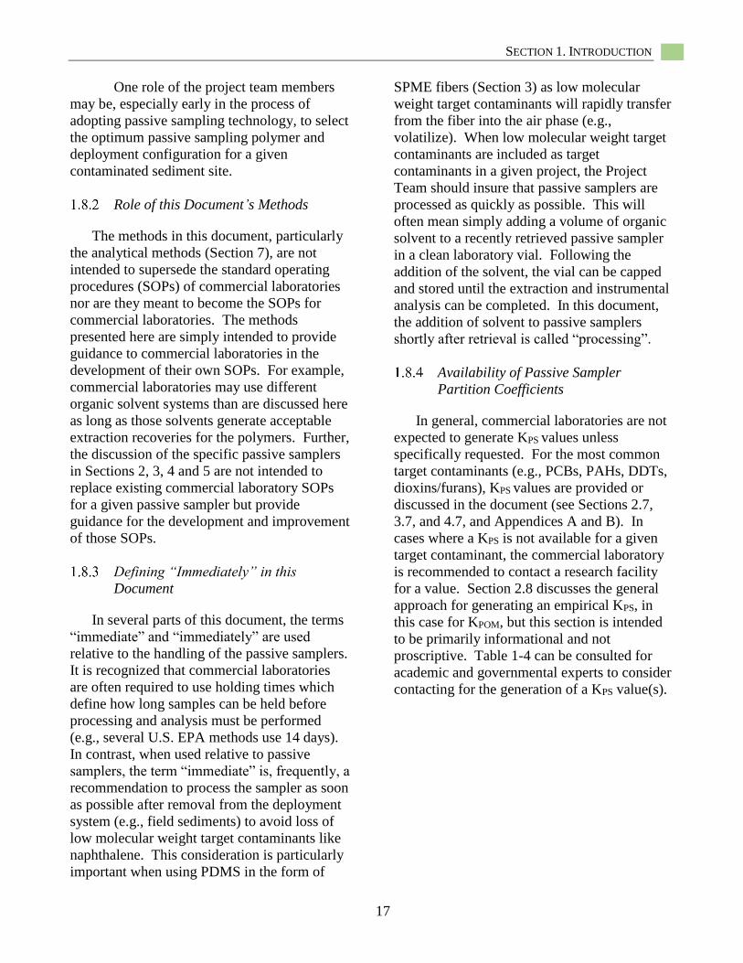
SECTION 1. INTRODUCTION
17
One role of the project team members
may be, especially early in the process of
adopting passive sampling technology, to select
the optimum passive sampling polymer and
deployment configuration for a given
contaminated sediment site.
Role of this Document’s Methods
The methods in this document, particularly
the analytical methods (Section 7), are not
intended to supersede the standard operating
procedures (SOPs) of commercial laboratories
nor are they meant to become the SOPs for
commercial laboratories. The methods
presented here are simply intended to provide
guidance to commercial laboratories in the
development of their own SOPs. For example,
commercial laboratories may use different
organic solvent systems than are discussed here
as long as those solvents generate acceptable
extraction recoveries for the polymers. Further,
the discussion of the specific passive samplers
in Sections 2, 3, 4 and 5 are not intended to
replace existing commercial laboratory SOPs
for a given passive sampler but provide
guidance for the development and improvement
of those SOPs.
Defining “Immediately” in this
Document
In several parts of this document, the terms
“immediate” and “immediately” are used
relative to the handling of the passive samplers.
It is recognized that commercial laboratories
are often required to use holding times which
define how long samples can be held before
processing and analysis must be performed
(e.g., several U.S. EPA methods use 14 days).
In contrast, when used relative to passive
samplers, the term “immediate” is, frequently, a
recommendation to process the sampler as soon
as possible after removal from the deployment
system (e.g., field sediments) to avoid loss of
low molecular weight target contaminants like
naphthalene. This consideration is particularly
important when using PDMS in the form of
SPME fibers (Section 3) as low molecular
weight target contaminants will rapidly transfer
from the fiber into the air phase (e.g.,
volatilize). When low molecular weight target
contaminants are included as target
contaminants in a given project, the Project
Team should insure that passive samplers are
processed as quickly as possible. This will
often mean simply adding a volume of organic
solvent to a recently retrieved passive sampler
in a clean laboratory vial. Following the
addition of the solvent, the vial can be capped
and stored until the extraction and instrumental
analysis can be completed. In this document,
the addition of solvent to passive samplers
shortly after retrieval is called “processing”.
Availability of Passive Sampler
Partition Coefficients
In general, commercial laboratories are not
expected to generate KPS values unless
specifically requested. For the most common
target contaminants (e.g., PCBs, PAHs, DDTs,
dioxins/furans), KPS values are provided or
discussed in the document (see Sections 2.7,
3.7, and 4.7, and Appendices A and B). In
cases where a KPS is not available for a given
target contaminant, the commercial laboratory
is recommended to contact a research facility
for a value. Section 2.8 discusses the general
approach for generating an empirical KPS, in
this case for KPOM, but this section is intended
to be primarily informational and not
proscriptive. Table 1-4 can be consulted for
academic and governmental experts to consider
contacting for the generation of a KPS value(s).

PASSIVE SAMPLING: USER’S MANUAL
18
Table 1-2. Application of passive samplers at selected U.S. EPA Superfund sites where the target
contaminants of concern (COCs) are organic contaminants
Site
U.S. EPA
Region Application
Aniston PCB 4 Develop a dose-response curve for benthic toxicity studies
Berry’s Creek 2 Monitor remedy effectiveness of activated carbon (AC) application in
a pilot study
Brodhead Creek 3 Monitor transport of contaminants from ground water into interstitial
water (not deployed yet)
Diamond Alkali 2 Monitor cap effectiveness; develop dose-response curve for benthic
toxicity studies
Grand Calumet 5 Monitor cap effectiveness
Grasse River 2 Monitor transport of contaminants from sediment into water column;
Compare passive sampler accumulation to bioaccumulation
Lake Hartwell 4 Monitor PCB diffusion from surficial sediment into overlying surface
water
Lower Duwamish
Waterway
10 Identify sources of contaminants to water column and organisms;
Monitor pilot study of activated carbon application effectiveness
MW
Manufacturing
3 Monitor volatile organic contaminant discharges from groundwater into
stream
Naval Station
Newport
1 Research and development on performance of passive sampling
methods
New Bedford
Harbor
1 Research and development on performance of passive sampling
methods
Pacific Sound
Resources
10 Assess groundwater breakthrough of a sediment cap via measurement of
interstitial water
Palos Verdes Shelf 9 Monitor transport of contaminants from sediment into water column;
remedy effectiveness
Tennessee
Products
4 Monitor creosote/non-aqueous phase liquid (NAPL) isolation (and
potential break thru) below a AquaBlok cap
United Heckathorn 9 Identify sources of contaminants to water column and organisms
Wyckoff 10 Monitor cap; Assess remedy effectiveness
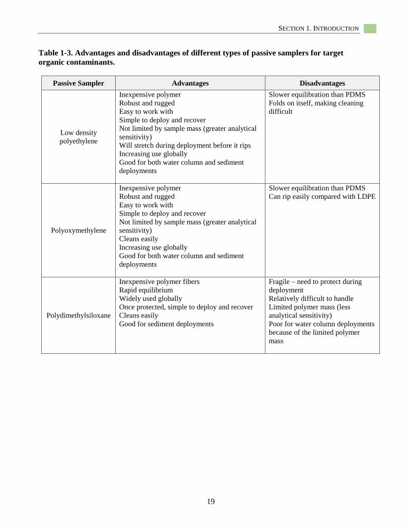
SECTION 1. INTRODUCTION
19
Table 1-3. Advantages and disadvantages of different types of passive samplers for target
organic contaminants.
Passive Sampler Advantages Disadvantages
Low density
polyethylene
Inexpensive polymer
Robust and rugged
Easy to work with
Simple to deploy and recover
Not limited by sample mass (greater analytical
sensitivity)
Will stretch during deployment before it rips
Increasing use globally
Good for both water column and sediment
deployments
Slower equilibration than PDMS
Folds on itself, making cleaning
difficult
Polyoxymethylene
Inexpensive polymer
Robust and rugged
Easy to work with
Simple to deploy and recover
Not limited by sample mass (greater analytical
sensitivity)
Cleans easily
Increasing use globally
Good for both water column and sediment
deployments
Slower equilibration than PDMS
Can rip easily compared with LDPE
Polydimethylsiloxane
Inexpensive polymer fibers
Rapid equilibrium
Widely used globally
Once protected, simple to deploy and recover
Cleans easily
Good for sediment deployments
Fragile – need to protect during
deployment
Relatively difficult to handle
Limited polymer mass (less
analytical sensitivity)
Poor for water column deployments
because of the limited polymer
mass
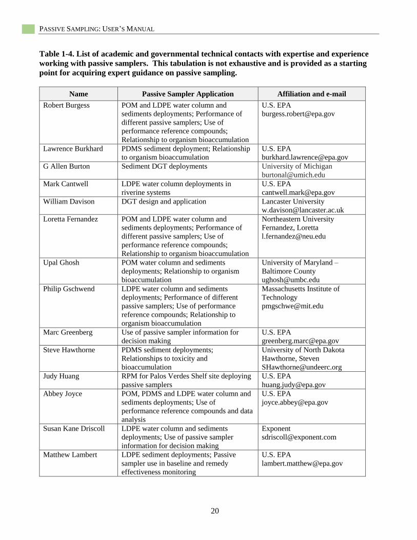
PASSIVE SAMPLING: USER’S MANUAL
20
Table 1-4. List of academic and governmental technical contacts with expertise and experience
working with passive samplers. This tabulation is not exhaustive and is provided as a starting
point for acquiring expert guidance on passive sampling.
Name Passive Sampler Application Affiliation and e-mail
Robert Burgess POM and LDPE water column and
sediments deployments; Performance of
different passive samplers; Use of
performance reference compounds;
Relationship to organism bioaccumulation
U.S. EPA
Lawrence Burkhard PDMS sediment deployment; Relationship
to organism bioaccumulation
U.S. EPA
G Allen Burton Sediment DGT deployments University of Michigan
Mark Cantwell LDPE water column deployments in
riverine systems
U.S. EPA
William Davison DGT design and application Lancaster University
Loretta Fernandez POM and LDPE water column and
sediments deployments; Performance of
different passive samplers; Use of
performance reference compounds;
Relationship to organism bioaccumulation
Northeastern University
Fernandez, Loretta
Upal Ghosh POM water column and sediments
deployments; Relationship to organism
bioaccumulation
University of Maryland –
Baltimore County
Philip Gschwend LDPE water column and sediments
deployments; Performance of different
passive samplers; Use of performance
reference compounds; Relationship to
organism bioaccumulation
Massachusetts Institute of
Technology
Marc Greenberg Use of passive sampler information for
decision making
U.S. EPA
Steve Hawthorne PDMS sediment deployments;
Relationships to toxicity and
bioaccumulation
University of North Dakota
Hawthorne, Steven
Judy Huang RPM for Palos Verdes Shelf site deploying
passive samplers
U.S. EPA
Abbey Joyce POM, PDMS and LDPE water column and
sediments deployments; Use of
performance reference compounds and data
analysis
U.S. EPA
Susan Kane Driscoll LDPE water column and sediments
deployments; Use of passive sampler
information for decision making
Exponent
Matthew Lambert LDPE sediment deployments; Passive
sampler use in baseline and remedy
effectiveness monitoring
U.S. EPA

SECTION 1. INTRODUCTION
21
Name Passive Sampler Application Affiliation and e-mail
Rainer Lohmann PDMS and LDPE water column and
sediments deployments; Performance of
different passive samplers; Use of
performance reference compounds
University of Rhode Island
Keith Maruya PDMS and LDPE water column and
sediments deployments; Use of
performance reference compounds;
Relationship to organism bioaccumulation
Southern California Coastal
Water Research Project
Keith Maruya
Marc Mills LDPE water column and sediment
deployments; Source tracking and
identification; Relationship to organism
bioaccumulation
U.S. EPA
Monique Perron LDPE, POM and PDMS water column and
sediments deployments; Performance of
different passive samplers; Use of
performance reference compounds
U.S. EPA
Danny Reible PDME water column and sediments
deployments; Relationship to organism
bioaccumulation
Texas Technical University
Sean Sheldrake Passive sampler deployment techniques and
diver related QA/QC issues
U.S. EPA
Stuart Simpson DGT application in marine sediments CISRO
Rachelle Thompson RPM for United Heckathorn site deploying
passive samplers
U.S. EPA

PASSIVE SAMPLING: USER’S MANUAL
22
Table 1-5. Examples of commercial analytical laboratories capable of consulting on and/
or performing analyses on passive samplers (as of December 2016). This tabulation is not exhaustive and is provided as a starting point for locating commercial laboratories with passive sampling experience.
Laboratory Contact Name and Location
ALS
Environmental
Jeff Christian
1317 South 13th Ave
Kelso WA 98626 USA
Alpha Analytical Jim Occhialini
8 Walkup Drive
Westborough, MA 01581
USA
AXYS Analytical
Services
Georgina Brooks
Richard Grace
2045 Mills Road West
Sidney, BC V8L 5X2
Canada
Brooksrand Labs Michelle Briscoe
[email protected] 18804 North Creek Parkway
Suite 100
Bothell, WA 98011 USA
DGT Research Ltd. Hao Zhang
Skelmorlie, Bay Horse Rd
Quernmore, Lancaster
Lancashire, LA2 0QJ
United Kingdom
Frontier Analytical
Laboratory
Bradley Silverbush
5172 Hillsdale Circle
El Dorado Hills, CA 95762 USA
Geosyntec Jason Conder
2100 Main Street, Suite 150
Huntington Beach, CA 92648 USA
PACE Analytical
Services, Inc.
Mary Christie
205 Seagull Dr.
Mosinee, WI 54455 USA
Test America Patricia MacIsaac
Bruce Wagner
3452 Lyrac St.
Oakton, VA 22124 USA
SiRem Jeff Roberts
130 Stone Road West
Guelph, Ontario N1G 3Z2
SECTION 1. INTRODUCTION
23
Table 1-6. Additional costs for commercial laboratories associated with the deployment and
analysis of passive samplers.
Scope of Activity Consideration
Labor of Laboratory Project Manager Additional labor may be necessary, especially early
in the process of adopting passive sampling when the
technology is unfamiliar.
Purchasing and cleaning passive samplers New costs.
Purchasing performance reference compounds
(PRCs)
New cost which can be expensive for the 13C-labelled
PRCs used for PCBs and DDTs. Use of deuterated
PAHs as PRCs for PAH passive sampling is much
less expensive than 13C-labelled PRCs.
Labor associated with amending passive samplers
with PRCs and verifying PRC concentrations in
passive samplers
New costs.
Additional labor and purchasing associated with
passive sampling analytical and QA/QC
requirements including passive samplers,
deployment, retrieval and field blanks, method
blanks, and matrix spikes and duplicates
New costs which will likely evolve as the use of
passive sampling becomes more familiar.
Document Overview
This User’s Manual has 10 sections and an
extensive selection of appendices. Following
this Introduction. The first four sections
discuss in detail the preparation, deployment,
and retrieval of POM, PDMS, LDPE, and DGT
passive samplers. The next sections address
the use of performance reference compounds
(PRCs), the extraction and analysis of passive
samplers, data analysis, and quality assurance
and quality control. The final section provides
an extensive list of the references cited
throughout this document. A series of
appendices provides a range of information,
including provisional partition coefficients for
POM, PDMS, and LDPE, passive sampling
case studies, and two examples of passive
sampler quality assurance project plans
(QAPPs).
Again, the primary goal of this document is
to provide the passive sampling user with the
information needed to deploy, collect and
analyze passive samplers and the resulting data.
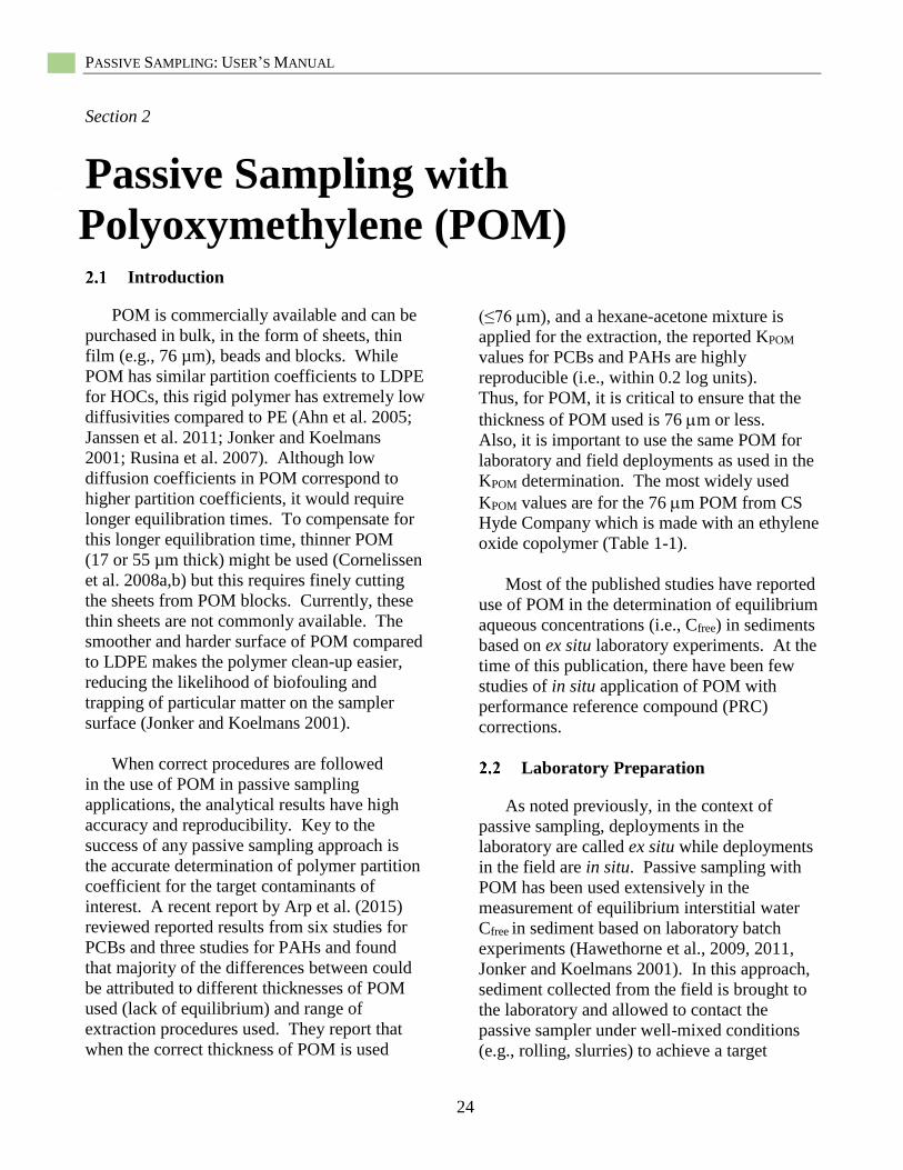
PASSIVE SAMPLING: USER’S MANUAL
24
Section 2
Passive Sampling with
Polyoxymethylene (POM) Introduction
POM is commercially available and can be
purchased in bulk, in the form of sheets, thin
film (e.g., 76 µm), beads and blocks. While
POM has similar partition coefficients to LDPE
for HOCs, this rigid polymer has extremely low
diffusivities compared to PE (Ahn et al. 2005;
Janssen et al. 2011; Jonker and Koelmans
2001; Rusina et al. 2007). Although low
diffusion coefficients in POM correspond to
higher partition coefficients, it would require
longer equilibration times. To compensate for
this longer equilibration time, thinner POM
(17 or 55 µm thick) might be used (Cornelissen
et al. 2008a,b) but this requires finely cutting
the sheets from POM blocks. Currently, these
thin sheets are not commonly available. The
smoother and harder surface of POM compared
to LDPE makes the polymer clean-up easier,
reducing the likelihood of biofouling and
trapping of particular matter on the sampler
surface (Jonker and Koelmans 2001).
When correct procedures are followed
in the use of POM in passive sampling
applications, the analytical results have high
accuracy and reproducibility. Key to the
success of any passive sampling approach is
the accurate determination of polymer partition
coefficient for the target contaminants of
interest. A recent report by Arp et al. (2015)
reviewed reported results from six studies for
PCBs and three studies for PAHs and found
that majority of the differences between could
be attributed to different thicknesses of POM
used (lack of equilibrium) and range of
extraction procedures used. They report that
when the correct thickness of POM is used
(≤76 m), and a hexane-acetone mixture is
applied for the extraction, the reported KPOM
values for PCBs and PAHs are highly
reproducible (i.e., within 0.2 log units).
Thus, for POM, it is critical to ensure that the
thickness of POM used is 76 m or less.
Also, it is important to use the same POM for
laboratory and field deployments as used in the
KPOM determination. The most widely used
KPOM values are for the 76 m POM from CS
Hyde Company which is made with an ethylene
oxide copolymer (Table 1-1).
Most of the published studies have reported
use of POM in the determination of equilibrium
aqueous concentrations (i.e., Cfree) in sediments
based on ex situ laboratory experiments. At the
time of this publication, there have been few
studies of in situ application of POM with
performance reference compound (PRC)
corrections.
Laboratory Preparation
As noted previously, in the context of
passive sampling, deployments in the
laboratory are called ex situ while deployments
in the field are in situ. Passive sampling with
POM has been used extensively in the
measurement of equilibrium interstitial water
Cfree in sediment based on laboratory batch
experiments (Hawethorne et al., 2009, 2011,
Jonker and Koelmans 2001). In this approach,
sediment collected from the field is brought to
the laboratory and allowed to contact the
passive sampler under well-mixed conditions
(e.g., rolling, slurries) to achieve a target
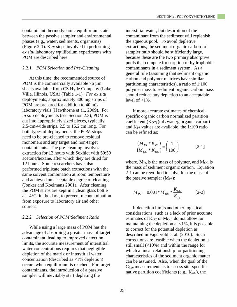
SECTION 2. POLYOXYMETHYLENE
25
contaminant thermodynamic equilibrium state
between the passive sampler and environmental
phases (e.g., water, sediments, organisms)
(Figure 2-1). Key steps involved in performing
ex situ laboratory equilibrium experiments with
POM are described here.
POM Selection and Pre-Cleaning
At this time, the recommended source of
POM is the commercially available 76 µm
sheets available from CS Hyde Company (Lake
Villa, Illinois, USA) (Table 1-1). For ex situ
deployments, approximately 300 mg strips of
POM are prepared for addition to 40 mL
laboratory vials (Hawthorne et al., 2009). For
in situ deployments (see Section 2.3), POM is
cut into appropriately sized pieces, typically
2.5-cm-wide strips, 2.5 to 15.2 cm long. For
both types of deployments, the POM strips
need to be pre-cleaned to remove residual
monomers and any target and non-target
contaminants. The pre-cleaning involves
extraction for 12 hours with Soxhlet with 50:50
acetone/hexane, after which they are dried for
12 hours. Some researchers have also
performed triplicate batch extractions with the
same solvent combination at room temperature
and achieved an acceptable degree of cleaning
(Jonker and Koelmans 2001). After cleaning,
the POM strips are kept in a clean glass bottle
at –4°C, in the dark, to prevent recontamination
from exposure to laboratory air and other
sources.
Selection of POM:Sediment Ratio
While using a large mass of POM has the
advantage of absorbing a greater mass of target
contaminant, leading to improved detection
limits, the accurate measurement of interstitial
water concentrations requires that negligible
depletion of the matrix or interstitial water
concentration (described as <1% depletion)
occurs when equilibrium is reached. For target
contaminants, the introduction of a passive
sampler will inevitably start depleting the
interstitial water, but desorption of the
contaminant from the sediment will replenish
the aqueous pool. To avoid depletive
extractions, the sediment organic carbon-to-
sampler ratio should be sufficiently large,
because these are the two primary absorptive
pools that compete for sorption of hydrophobic
contaminants in a sediment system. As a
general rule (assuming that sediment organic
carbon and polymer matrices have similar
partitioning characteristics), a ratio of 1:100
polymer mass to sediment organic carbon mass
should reduce any depletion to an acceptable
level of <1%.
If more accurate estimates of chemical-
specific organic carbon normalized partition
coefficient (KOC) (mL waer/g organic carbon)
and KPS values are available, the 1:100 ratio
can be refined as:
100
1
*
*
OCOC
PSPS
KM
KM[2-1]
where, MPS is the mass of polymer, and MOC is
the mass of sediment organic carbon. Equation
2-1 can be reworked to solve for the mass of
the passive sampler (MPS):
PS
OC
OCPSK
KMM **001.0 [2-2]
If detection limits and other logistical
considerations, such as a lack of prior accurate
estimates of KOC or MOC, do not allow for
maintaining the depletion at <1%, it is possible
to correct for the potential depletion as
described in Fagervold et al. (2010). Such
corrections are feasible when the depletion is
still small (<10%) and within the range for
which a linear relationship for partitioning
characteristics of the sediment organic matter
can be assumed. Also, when the goal of the
Cfree measurements is to assess site-specific
native partition coefficients (e.g., KOC), the
PASSIVE SAMPLING: USER’S MANUAL
26
decreased matrix concentrations (i.e., post-
deployment sediment concentrations) can be
measured and accounted for in the partitioning
calculation.
Selection of Sediment Mass to be used
for Cfree Determinations
Key criteria that are involved in deciding
how much sediment mass should be used
include the concentration of the target
contaminant in the sediment and the analytical
detection limits. One approach for performing
the calculation is to work backward from the
analytical mass detection limits. For example,
if the analytical detection limit is X ng/mL for
a given target contaminant in the final solvent
extract, and the desire is to stay 10 times above
the detection limit, one can target a final
concentration of 10X ng/mL as the minimum.
Assuming a final extract volume of 1 mL, this
amounts to a mass of 10X ng target
contaminant sampled in the POM. The batch
equilibrium experiments are designed such that
not more than 1% of the target contaminant is
transferred from the sediment into the passive
sampler, as described above. Thus, the
minimum sediment mass that is required should
have 1000X ng of the target contaminant.
So, the mass of sediment required will equal
1000X/Csed g, where Csed [ng/g] is the
concentration of the target contaminant in
sediment. For most applications, this results in
the range of 10–1000 g sediment (wet) per
replicate measurement depending on the level
of sediment contamination. For example,
Hawthorne et al., (2009) used 10 to 15 grams of
relatively highly PCB contaminated wet
sediment combined with 30 mL of deionized
water to perform their ex situ sediment-water
slurry equilibrations (Figure 2-1). The
sediment sample should be homogenized
before distributing into at least duplicate
samples (n = 2) for the measurement of
equilibrium interstitial water Cfree.
Exposure Time and Conditions
A typical exposure time for well-mixed
batch experiments with POM is one month.
Results reported by Hawthorne et al. (2009)
indicate adequate equilibration even for
octachlorobiphenyls in that period of time in
well-mixed batch systems. While sediment
samples with high water content can be used
directly to form a slurry, additional water may
need to be added to form a free-flowing slurry
for most sediments. Typical water content in a
well-formed slurry is 80% water (Figure 2-1).
Clean DI water can be used to supplement the
water content for freshwater sediments. If
necessary, water with appropriate salinity can
be prepared by adding reconstituted seawater
prepared from hypersaline brine or Instant
Ocean salt mixture, as performed by Gomez-
Eyles et al. (2013). Exposure bottles should be
well mixed, typically on a shaker table or bottle
roller mill during the equilibration. The
purpose of the mixing is to reduce the aqueous
boundary-layer thickness around the sediment
particles and the passive sampler to enhance
target contaminant mass transfer.
Use of Biocides to Inhibit Target
Contaminant Biodegradation
For degradable target contaminants (e.g.,
PAHs), biocides such as sodium azide (100–
1000 mg/L) (Cornelissen et al. 2006; Khalil et
al. 2006; Zimmerman et al. 2004) or mercuric
chloride are required to inhibit biological
activity during the experiments. In addition,
the experiments should be conducted in the
dark or in amber bottles to reduce the chance of
photodegradation of some target contaminants.
SECTION 2. POLYOXYMETHYLENE
27
Field Use
In situ Deployment Device Designs
An important difference in the field
deployment is the physical deployment device
used to protect the sampler from harsh
environmental conditions or damage during
deployment and recovery in sediments. While
POM is more rigid than other polymers, such as
LDPE and PDMS, the thin POM strips can
easily fold up during deployment if they are not
adequately supported. Although unframed
POM strips have been used by Cornelissen et
al. (2008b) and Beckingham et al. (2013) for
surface water measurements, for deployment
within sediment, the POM sampler is typically
encased in a stainless-steel fine mesh and a
metal frame such as shown in Figure 2-2.
Stainless steel is a suitable metal for use in field
deployments, because it resists corrosion
adequately. While galvanized iron or
aluminum may work for short deployment
periods, both are prone to corrosion, especially
in saltwater environments. To date, POM
samplers have been deployed by wading to the
station or by divers as well as attaching POM
passive samplers to metal frames fastened to a
platform lowered into the seabed at depths
exceeding diver limitations (e.g., 60 m) (see
Figure 4-4c) (Fernandez et al., 2014).
Additional details on field deployment is
provided in Appendix F, Case Study 1. As
noted in Section 1 (Figure 1-5), in areas where
vandalism is a concern, rather than using
surface buoys to mark passive samplers, lines
can be returned to shore or the application of
subsurface buoys may be considered.
Recovery and Processing
POM passive sampling strips deployed
in laboratory or field exposures should be
removed from any enclosures and rinsed with
deionized water to remove attached sediment.
The POM strips should be wiped gently with
clean laboratory wipes to remove any attached
biological growth, and rinsed again with DI
water. Do not use any alcohol or solvent-
soaked swabs. Note that some discoloration
from iron oxide deposits may be difficult to
remove, but it is not expected to influence the
sorption of target contaminants. The strips
should be wiped dry and stored in clean glass
vials in a freezer at –4°C, in the dark, until they
are analyzed.
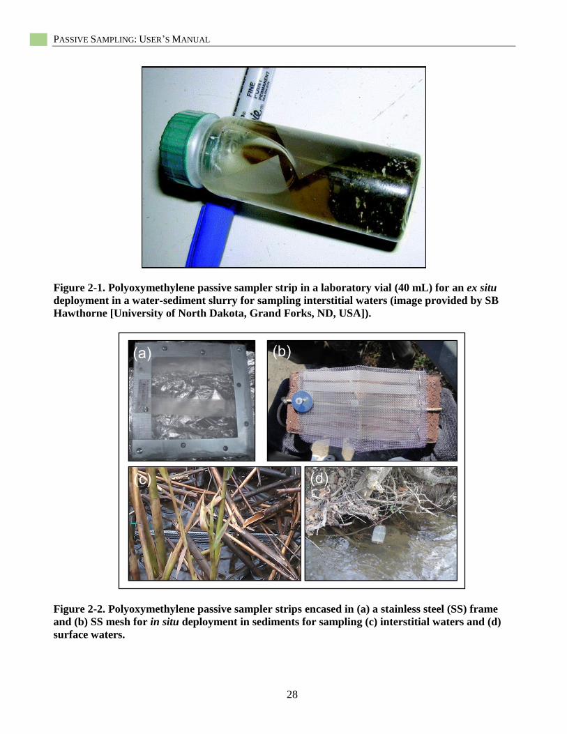
PASSIVE SAMPLING: USER’S MANUAL
28
Figure 2-1. Polyoxymethylene passive sampler strip in a laboratory vial (40 mL) for an ex situ
deployment in a water-sediment slurry for sampling interstitial waters (image provided by SB
Hawthorne [University of North Dakota, Grand Forks, ND, USA]).
Figure 2-2. Polyoxymethylene passive sampler strips encased in (a) a stainless steel (SS) frame
and (b) SS mesh for in situ deployment in sediments for sampling (c) interstitial waters and (d)
surface waters.
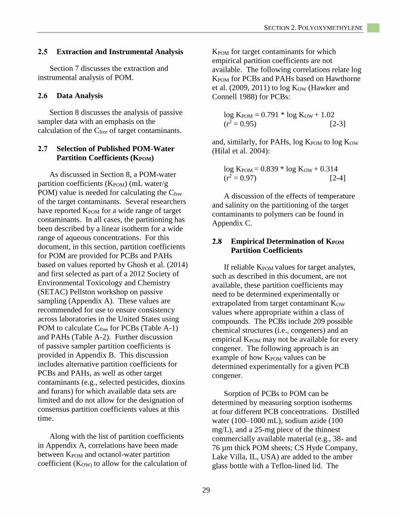
SECTION 2. POLYOXYMETHYLENE
29
Extraction and Instrumental Analysis
Section 7 discusses the extraction and
instrumental analysis of POM.
Data Analysis
Section 8 discusses the analysis of passive
sampler data with an emphasis on the
calculation of the Cfree of target contaminants.
Selection of Published POM-Water
Partition Coefficients (KPOM)
As discussed in Section 8, a POM-water
partition coefficients (KPOM) (mL water/g
POM) value is needed for calculating the Cfree
of the target contaminants. Several researchers
have reported KPOM for a wide range of target
contaminants. In all cases, the partitioning has
been described by a linear isotherm for a wide
range of aqueous concentrations. For this
document, in this section, partition coefficients
for POM are provided for PCBs and PAHs
based on values reported by Ghosh et al. (2014)
and first selected as part of a 2012 Society of
Environmental Toxicology and Chemistry
(SETAC) Pellston workshop on passive
sampling (Appendix A). These values are
recommended for use to ensure consistency
across laboratories in the United States using
POM to calculate Cfree for PCBs (Table A-1)
and PAHs (Table A-2). Further discussion
of passive sampler partition coefficients is
provided in Appendix B. This discussion
includes alternative partition coefficients for
PCBs and PAHs, as well as other target
contaminants (e.g., selected pesticides, dioxins
and furans) for which available data sets are
limited and do not allow for the designation of
consensus partition coefficients values at this
time.
Along with the list of partition coefficients
in Appendix A, correlations have been made
between KPOM and octanol-water partition
coefficient (KOW) to allow for the calculation of
KPOM for target contaminants for which
empirical partition coefficients are not
available. The following correlations relate log
KPOM for PCBs and PAHs based on Hawthorne
et al. (2009, 2011) to log KOW (Hawker and
Connell 1988) for PCBs:
log KPOM = 0.791 * log KOW + 1.02
(r2 = 0.95) [2-3]
and, similarly, for PAHs, log KPOM to log KOW
(Hilal et al. 2004):
log KPOM = 0.839 * log KOW + 0.314
(r2 = 0.97) [2-4]
A discussion of the effects of temperature
and salinity on the partitioning of the target
contaminants to polymers can be found in
Appendix C.
Empirical Determination of KPOM
Partition Coefficients
If reliable KPOM values for target analytes,
such as described in this document, are not
available, these partition coefficients may
need to be determined experimentally or
extrapolated from target contaminant KOW
values where appropriate within a class of
compounds. The PCBs include 209 possible
chemical structures (i.e., congeners) and an
empirical KPOM may not be available for every
congener. The following approach is an
example of how KPOM values can be
determined experimentally for a given PCB
congener.
Sorption of PCBs to POM can be
determined by measuring sorption isotherms
at four different PCB concentrations. Distilled
water (100–1000 mL), sodium azide (100
mg/L), and a 25-mg piece of the thinnest
commercially available material (e.g., 38- and
76 µm thick POM sheets; CS Hyde Company,
Lake Villa, IL, USA) are added to the amber
glass bottle with a Teflon-lined lid. The
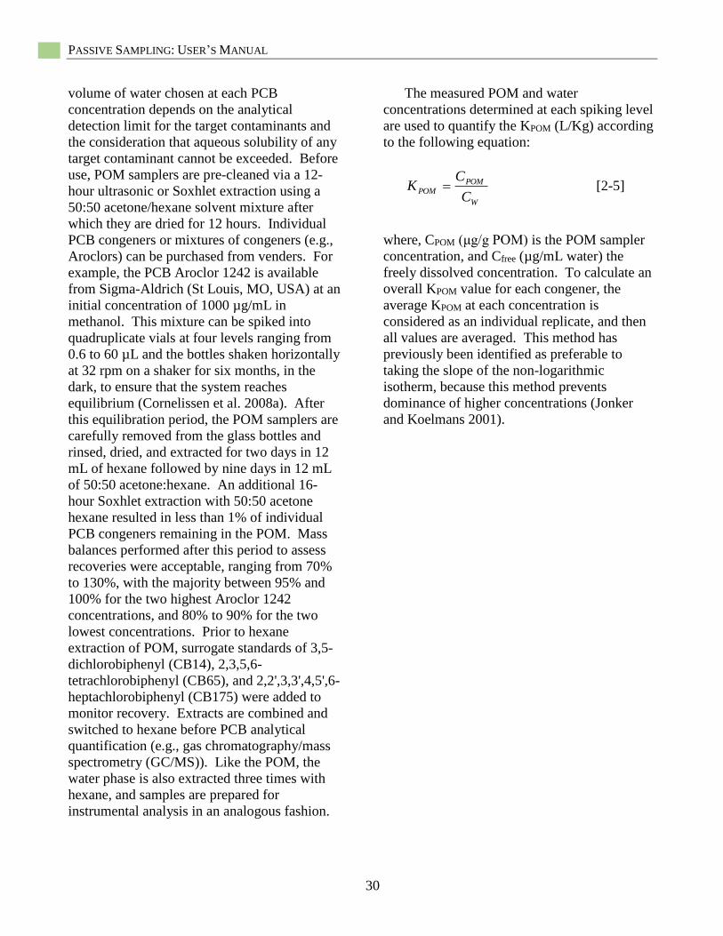
PASSIVE SAMPLING: USER’S MANUAL
30
volume of water chosen at each PCB
concentration depends on the analytical
detection limit for the target contaminants and
the consideration that aqueous solubility of any
target contaminant cannot be exceeded. Before
use, POM samplers are pre-cleaned via a 12-
hour ultrasonic or Soxhlet extraction using a
50:50 acetone/hexane solvent mixture after
which they are dried for 12 hours. Individual
PCB congeners or mixtures of congeners (e.g.,
Aroclors) can be purchased from venders. For
example, the PCB Aroclor 1242 is available
from Sigma-Aldrich (St Louis, MO, USA) at an
initial concentration of 1000 µg/mL in
methanol. This mixture can be spiked into
quadruplicate vials at four levels ranging from
0.6 to 60 µL and the bottles shaken horizontally
at 32 rpm on a shaker for six months, in the
dark, to ensure that the system reaches
equilibrium (Cornelissen et al. 2008a). After
this equilibration period, the POM samplers are
carefully removed from the glass bottles and
rinsed, dried, and extracted for two days in 12
mL of hexane followed by nine days in 12 mL
of 50:50 acetone:hexane. An additional 16-
hour Soxhlet extraction with 50:50 acetone
hexane resulted in less than 1% of individual
PCB congeners remaining in the POM. Mass
balances performed after this period to assess
recoveries were acceptable, ranging from 70%
to 130%, with the majority between 95% and
100% for the two highest Aroclor 1242
concentrations, and 80% to 90% for the two
lowest concentrations. Prior to hexane
extraction of POM, surrogate standards of 3,5-
dichlorobiphenyl (CB14), 2,3,5,6-
tetrachlorobiphenyl (CB65), and 2,2',3,3',4,5',6-
heptachlorobiphenyl (CB175) were added to
monitor recovery. Extracts are combined and
switched to hexane before PCB analytical
quantification (e.g., gas chromatography/mass
spectrometry (GC/MS)). Like the POM, the
water phase is also extracted three times with
hexane, and samples are prepared for
instrumental analysis in an analogous fashion.
The measured POM and water
concentrations determined at each spiking level
are used to quantify the KPOM (L/Kg) according
to the following equation:
W
POM
POMC
CK [2-5]
where, CPOM (μg/g POM) is the POM sampler
concentration, and Cfree (µg/mL water) the
freely dissolved concentration. To calculate an
overall KPOM value for each congener, the
average KPOM at each concentration is
considered as an individual replicate, and then
all values are averaged. This method has
previously been identified as preferable to
taking the slope of the non-logarithmic
isotherm, because this method prevents
dominance of higher concentrations (Jonker
and Koelmans 2001).
SECTION 3. POLYDIMETHYLSILOXANE
31
Section 3
Passive Sampling with
Polydimethylsiloxane (PDMS) Introduction
Currently, the most common form of
polydimethylsiloxane (PDMS) passive sampler,
solid-phase microextraction (SPME) uses a
hollow fused silica optical fiber coated with the
polymer (Figure 3-1). Initially developed as a
sample extraction tool for analytical chemistry,
SPME with PDMS has been adapted as an
environmental passive sampling technique
(Arthur and Pawliszyn 1990; Kraaij et al. 2002;
Mayer et al. 2000; Smedes and Booij 2012).
The thin PDMS coating over a relatively long
fiber renders higher surface area-to-volume
ratio, which enables PDMS to reach
equilibrium faster than PE or POM. For
example, long fibers with proper protective
casing can be used to monitor the vertical
profile of sediment interstitial water
contamination (Lampert et al. 2013; Lampert
et al. 2011). Concern for the fiber’s potential
fragility should be addressed when
deployments are in harsh environments. For
field applications, the thinner fibers are not as
robust as the relatively simple passive sampling
polymer sheets (e.g., POM, LDPE) and are
often deployed in a protected form to avoid loss
or breakage (e.g., metal mesh, copper or
stainless steel sheath or tubing).
Although not the focus of this document,
there are two additional PDMS-based passive
sampling techniques worth noting. The first is
an ex situ method developed by Hawthorne et
al. (2005) in which SPME fibers are placed into
a small volume (i.e., < 10 mL) of isolated
interstitial water treated to remove colloidal
matter. Under these conditions, the SPME
fiber absorbs freely dissolved target
contaminants. This method is not an
equilibrium passive sampling method like the
others described for nonpolar organic target
contaminants in this document as other
environmental phases have been removed.
The method rapidly accumulates target
contaminants on the SPME fiber resulting in
low detection limits. The second additional
method is also an ex situ technique involving
coating jars with a thin layer of PDMS
(Reichenberg et al. 2008; Jahnke et al. 2012).
Contaminated sediments added to the jars are
rolled to establish equilibrium between the
target contaminants and the PDMS coating.
Coatings of different thicknesses of PDMS
allow for the determination of equilibrium
conditions.

PASSIVE SAMPLING: USER’S MANUAL
32
Figure 3-1. Schematic of solid phase microextraction fiber showing the outer coating of poly-
dimethylsiloxane (from U.S. EPA 2012b). Dimensions are presented as examples only.
Figure 3-2. Insertion of a PDMS coated SPME fiber into whole sediments (in a 20 mL
scintillation vial) for an ex situ deployment.
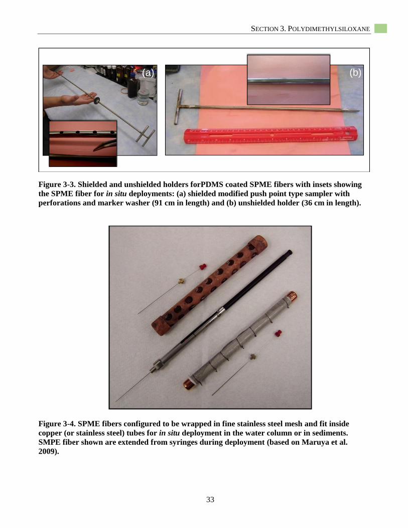
SECTION 3. POLYDIMETHYLSILOXANE
33
(a) (b)
Figure 3-3. Shielded and unshielded holders forPDMS coated SPME fibers with insets showing
the SPME fiber for in situ deployments: (a) shielded modified push point type sampler with
perforations and marker washer (91 cm in length) and (b) unshielded holder (36 cm in length).
Figure 3-4. SPME fibers configured to be wrapped in fine stainless steel mesh and fit inside
copper (or stainless steel) tubes for in situ deployment in the water column or in sediments.
SMPE fiber shown are extended from syringes during deployment (based on Maruya et al.
2009).
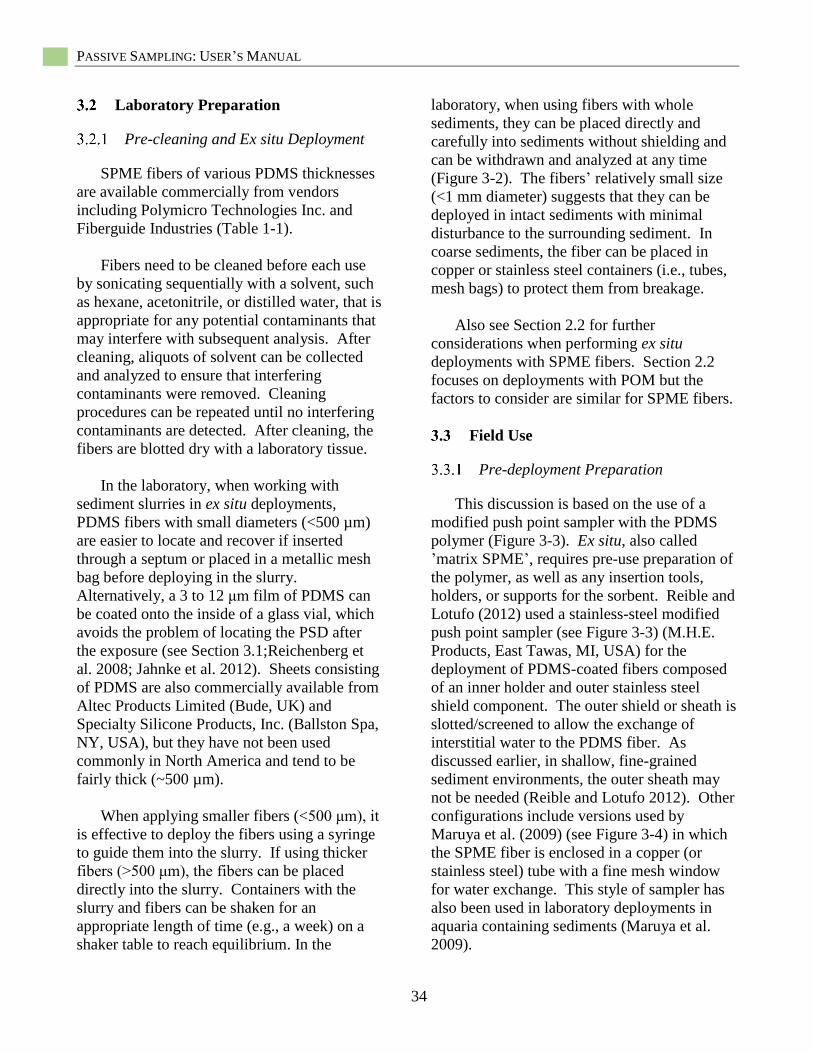
PASSIVE SAMPLING: USER’S MANUAL
34
Laboratory Preparation
Pre-cleaning and Ex situ Deployment
SPME fibers of various PDMS thicknesses
are available commercially from vendors
including Polymicro Technologies Inc. and
Fiberguide Industries (Table 1-1).
Fibers need to be cleaned before each use
by sonicating sequentially with a solvent, such
as hexane, acetonitrile, or distilled water, that is
appropriate for any potential contaminants that
may interfere with subsequent analysis. After
cleaning, aliquots of solvent can be collected
and analyzed to ensure that interfering
contaminants were removed. Cleaning
procedures can be repeated until no interfering
contaminants are detected. After cleaning, the
fibers are blotted dry with a laboratory tissue.
In the laboratory, when working with
sediment slurries in ex situ deployments,
PDMS fibers with small diameters (<500 µm)
are easier to locate and recover if inserted
through a septum or placed in a metallic mesh
bag before deploying in the slurry.
Alternatively, a 3 to 12 μm film of PDMS can
be coated onto the inside of a glass vial, which
avoids the problem of locating the PSD after
the exposure (see Section 3.1;Reichenberg et
al. 2008; Jahnke et al. 2012). Sheets consisting
of PDMS are also commercially available from
Altec Products Limited (Bude, UK) and
Specialty Silicone Products, Inc. (Ballston Spa,
NY, USA), but they have not been used
commonly in North America and tend to be
fairly thick (~500 µm).
When applying smaller fibers (<500 μm), it
is effective to deploy the fibers using a syringe
to guide them into the slurry. If using thicker
fibers (>500 μm), the fibers can be placed
directly into the slurry. Containers with the
slurry and fibers can be shaken for an
appropriate length of time (e.g., a week) on a
shaker table to reach equilibrium. In the
laboratory, when using fibers with whole
sediments, they can be placed directly and
carefully into sediments without shielding and
can be withdrawn and analyzed at any time
(Figure 3-2). The fibers’ relatively small size
(<1 mm diameter) suggests that they can be
deployed in intact sediments with minimal
disturbance to the surrounding sediment. In
coarse sediments, the fiber can be placed in
copper or stainless steel containers (i.e., tubes,
mesh bags) to protect them from breakage.
Also see Section 2.2 for further
considerations when performing ex situ
deployments with SPME fibers. Section 2.2
focuses on deployments with POM but the
factors to consider are similar for SPME fibers.
Field Use
Pre-deployment Preparation
This discussion is based on the use of a
modified push point sampler with the PDMS
polymer (Figure 3-3). Ex situ, also called
’matrix SPME’, requires pre-use preparation of
the polymer, as well as any insertion tools,
holders, or supports for the sorbent. Reible and
Lotufo (2012) used a stainless-steel modified
push point sampler (see Figure 3-3) (M.H.E.
Products, East Tawas, MI, USA) for the
deployment of PDMS-coated fibers composed
of an inner holder and outer stainless steel
shield component. The outer shield or sheath is
slotted/screened to allow the exchange of
interstitial water to the PDMS fiber. As
discussed earlier, in shallow, fine-grained
sediment environments, the outer sheath may
not be needed (Reible and Lotufo 2012). Other
configurations include versions used by
Maruya et al. (2009) (see Figure 3-4) in which
the SPME fiber is enclosed in a copper (or
stainless steel) tube with a fine mesh window
for water exchange. This style of sampler has
also been used in laboratory deployments in
aquaria containing sediments (Maruya et al.
2009).
SECTION 3. POLYDIMETHYLSILOXANE
35
Before loading the PDMS fiber into a
holder or placing them directly into the
sediments, the polymer and the holder must be
cleaned of any potential contamination. The
holder can often be scrubbed with hot water
and detergent and then rinsed sequentially with
solvents appropriate for the contaminants that
may interfere with subsequent analysis (e.g.,
hexane, acetonitrile, distilled water, or others).
The components are then dried (e.g., in an oven
overnight). The solvents used for cleaning are
typically the same as those used to extract the
PDMS after the exposure, which ensures that
the sampling equipment is free of contaminants
that are extractable by the analysis solvent.
Reible and Lotufo (2012) used acetonitrile as a
primary cleaning solvent when analyzing for
PAHs because acetonitrile was also used as
the carrier solvent for analysis of PAHs by high
performance liquid chromatography (HPLC)
with fluorescent detection. Similarly, Reible
and Lotufo (2012) used hexane as a primary
solvent for PCBs analysis, because their
GC/ECD analytical method used hexane as a
carrier solvent.
For deployed devices, the cleaned fibers
are laid into the groove of the inner holder
of the modified sampler and affixed with
approximately 1 cm of waterproof caulk
(hydrocarbon-free silicon) at both ends. Caulk
is used to hold the fiber in place, and can also
be used to fill any gaps between the holder and
the shield at the ends of the insertion tool, to
eliminate any vertical water movement. Care
should be taken to avoid any placement of
silicon on the screened length or active
measurement portion of the insertion tool.
Also avoid placing too much silicon, so that the
cured silicon hinders separation of the insertion
tool from the fiber or outer sheath after field
deployment. After the caulk dries, the inner
holder is inserted into the outer sheath, with
groove and fiber aligned with the screened side
of the sheath. The handles on both the inner
grooved holder and sheath are wrapped
together to maintain orientation of the fiber to
the screened section of the outer sheath. The
length of the fiber loaded into each insertion
tool is documented, and the samplers are
labeled via a waterproof marker.
In situ Deployment
For in situ field application of PDMS, the
fiber should be placed in an outer holder to
protect it from breakage. In coarse sediments
(gravel, rocky, or filled with debris) the holder
should include an external sheath to help
protect the fiber. As discussed previously, the
holder or sampler used herein is modified from
a hand-held piezometer (i.e., push point
sampler). Modifications include adding
perforations in the outer sheath to allow water
exchange, incorporation of a slit into the inner
sheath to hold the SPME fiber, and adding a
washer to mark the sediment/water interface
(Figure 3-3a). Fibers can be left unshielded for
short lengths (up to 30 cm) in soft sediments
(Figure 3-3b). Other types of samplers or fiber
holders are acceptable, as long as they can
protect the fiber from breakage, do not interfere
with water and fiber exchange, and can be
easily deployed.
In the field, use of PDMS fibers is more
complicated, because placement typically
requires divers, and shielding to protect the
fibers during placement. The modified push
point sampler based system was found to be
simple to deploy in all but the most difficult of
subsurface environments (e.g., sediments
armored by rock). The primary difficulty is
ensuring proper vertical placement, particularly
in soft sediments where the lack of resistance
of the sediment makes it difficult to define the
sediment/water interface. Retrieval by divers
or remotely by pulling on an attached line has
been demonstrated at multiple field locations.
However, as noted in Section 1.7, using divers
will involve special considerations including
appropriate personal protective equipment
(PPE) usage. Consulting with U.S. EPA
PASSIVE SAMPLING: USER’S MANUAL
36
experts on diver based deployment and
retrieval is recommended.
For in situ placement into sediment, the
assembled SPME insertion devices are driven
perpendicular into the sediment surface by
divers at locations not accessible on foot. An
alternative method uses a long, sleeved pipe to
insert the sampler into the sediment from the
surface. Samples can also be collected by
conventional cylindrical or box corer and
placed in the laboratory before insertion of the
sampler. Sampling in the laboratory is similar
to the field, except that the effects of field-
related processes such as groundwater
upwelling and tides will not be included.
All SPME insertion devices are marked
during deployment to allow retrieval. This
might include cording to surface-deployed
buoys or cording run to a nearby shore. The
samplers can be pushed into sediment by hand
at easily accessible sites (e.g., onshore locations
at low tide and shallow creeks). Deployment
blanks (also considered a field blank) can be
shipped to the field but not deployed, to assess
possible sources of contamination to the
sampler on site or during shipping. For SPME,
the deployment blanks should be processed
(i.e., transferred to vials and solvent added) at
the time of deployment. A field blank can also
be used for retrieval. No retrieval field blank is
needed if the samplers are processed on site
immediately after retrieval.
As noted in Section 1 (Figure 1-5) and
above, in areas where vandalism is a concern,
rather than using surface buoys to locate
passive samplers, lines can be returned to shore
or the application of subsurface buoys may be
considered.
Recovery and Processing
All fibers are typically equilibrated in situ for
7 to 28 days before retrieval. The equilibrium
time is chosen as a balance between using short
times to minimize sample disturbance or
vandalism and the time required to achieve a
significant fraction of equilibrium for highly
hydrophobic contaminants. Full equilibration
involves the initial depletion of the interstitial
water surrounding the fiber and then slow re-
equilibration with the surrounding media.
The time required to achieve full equilibrium
depends on the hydrophobicity of the target
contaminant being analyzed, the dimensions
of the PDMS polymer, and the mixing
characteristics within the sediment. A highly
hydrophobic contaminant (e.g., a tetrachloro-
or higher chlorinated biphenyl), in a medium
that is easily depleted due to low sorption
capacity (e.g., sand), under conditions of
limited transport (e.g., diffusion-controlled
conditions) may require well in excess of 28
days to achieve full equilibrium. A less
hydrophobic contaminant (e.g., 3- or 4-ring
PAH) may reach equilibrium within a period of
days in a typical fine-grained organic-rich, and
therefore high-capacity, sediment. Lampert et
al. (2015) discuss a modelling approach for
estimating how much time is required to
achieve equilibrium between the target
contaminants and the PDMS polymer.
After deploying the fibers for the specified
length of time in the sediment to be sampled,
they are removed from the sediment. It is
generally convenient to process the fibers
immediately, to maximize sample integrity.
Low-molecular-weight and volatile
contaminants (e.g., naphthalene or less
hydrophobic/more volatile chemicals) are not
easily measured, due to minimal concentrations
on the fiber and rapid volatilization on
exposure to the atmosphere.
Samplers deployed in the field are first
dismantled from the solid support (e.g., push
point sampler). The sorbent fiber is removed,
cleaned with water or a damp laboratory tissue
to remove any sediment particles, and either
placed on ice for shipment to the laboratory or

SECTION 3. POLYDIMETHYLSILOXANE
37
sectioned and placed into extracting solvent in
the field. Due to the relatively slow kinetics of
uptake or loss of target contaminants from the
sorbent when exposed to water, quick rinsing
will not alter the concentration on the sorbent.
Processing of PDMS fibers onsite by sectioning
and placing into auto-sampling vials with
inserts prefilled with aliquots of solvent is an
effective processing method that stabilizes the
samples for shipment to the processing
laboratory without concern for sample
degradation during transport.
The passive sampling materials can be
cut into different segment sizes based on the
objectives of a given project. For example,
sampling within the biologically active zone
(e.g., 0–10 cm) would characterize exposure to
benthic organisms, while sampling in deeper
segments (e.g., 10–20 cm, 20–30 cm, etc.) may
indicate potential migration from below into
the biologically active zone. Vertical diffusion
of contaminants along the PDMS fiber likely
limits vertical resolution to 1–2 cm, depending
on the time of exposure. Normally, adjacent
1- to 2-cm sample segments can be used as
duplicate samples under most environmental
conditions.
Any observances of color change and odor
of the passive sampling material or solid
support should be documented. Changes in
color may be due to changes in the
biogeochemistry of the sediment or the
presence of non-aqueous-phase liquids
(NAPLs) which can also be detected by odor.
Note that contact with NAPL can affect the
validity of the interstitial water measurements,
because the passive sampling material may
directly absorb the NAPL. This would cause
the concentration in the polymer sorbent to be
much higher than if the sorbent were exposed
only to water equilibrated with the same NAPL
phase. If NAPL contamination of the PDMS is
suspected, the calculation of Cfree should not be
performed as the derived values will likely be
over-estimations.
Extraction and Instrumental Analysis
The SPME fibers can be liquid extracted
like the other types of passive samplers (see
Section 7). However, unique to SPME, the
fibers can be cut into segments, followed by
placement into an auto-sampling vial with an
insert and aliquot of solvent, followed by
analysis via direct injection into the analytical
instrumentation (e.g., GC or HPLC) (see
Section 7). The lack of additional processing
steps when using direct injection is a major
advantage of the method, reducing time, cost,
and potential contaminant losses due to sample
cleanup or extraction steps.
Data Analysis
See Section 8.
Selection of Published PDMS-Water
Partition Coefficients (KPDMS)
Several researchers have reported PDMS-
water partition coefficients (KPDMS) for a wide
range of target contaminants. In all cases, the
partitioning has been described by a linear
isotherm for a wide range of aqueous
concentrations. For this section, partition
coefficients for PDMS are provided for PCBs
and PAHs based on values reported by Ghosh
et al. (2014) and first selected as part of a 2012
Society of Environmental Toxicology and
Chemistry (SETAC) Pellston workshop on
passive sampling (Appendix A). These values
are recommended for use to ensure consistency
across laboratories in the United States using
PDME to calculate Cfree for PCBs (Table A-1)
and PAHs (Table A-2). Further discussion of
passive sampler partition coefficients is
provided in Appendix B. This discussion
includes alternative partition coefficients for
PCBs and PAHs, as well as other target
contaminants (e.g., selected pesticides, dioxins,
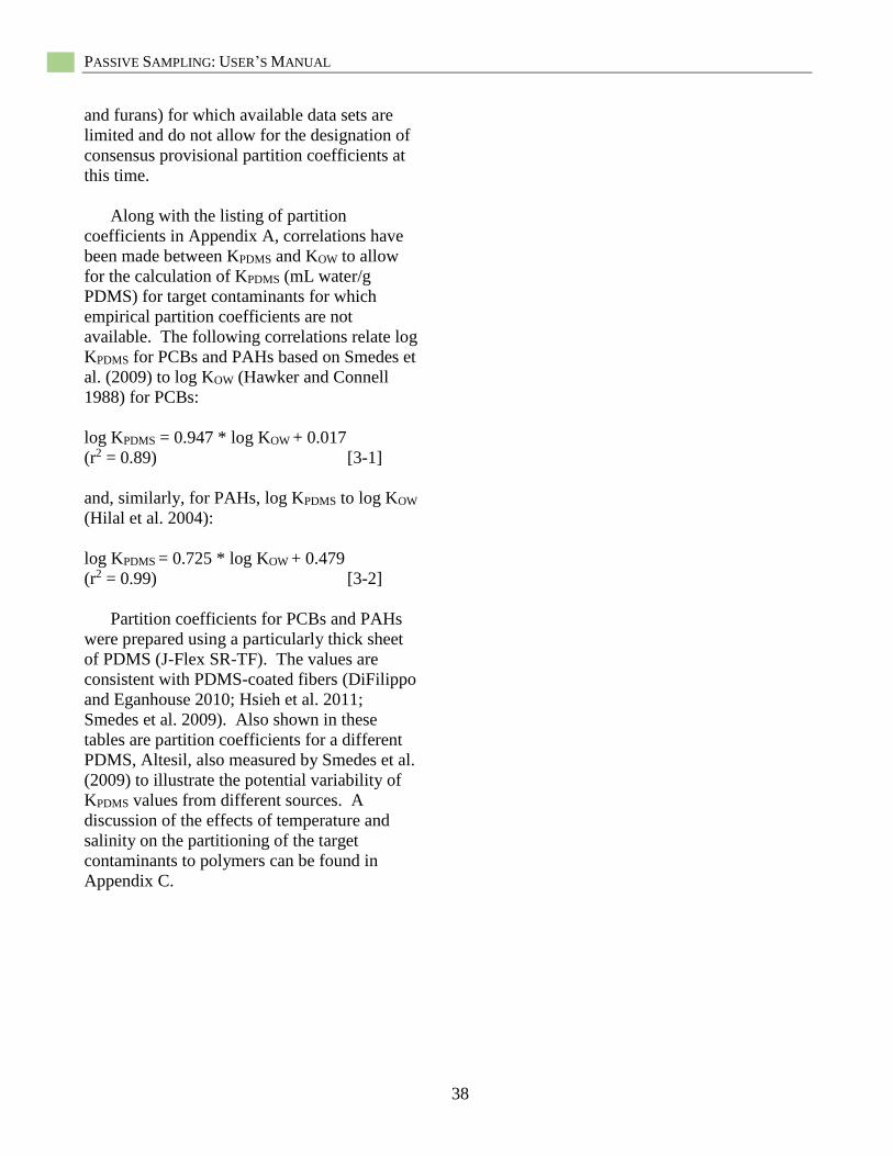
PASSIVE SAMPLING: USER’S MANUAL
38
and furans) for which available data sets are
limited and do not allow for the designation of
consensus provisional partition coefficients at
this time.
Along with the listing of partition
coefficients in Appendix A, correlations have
been made between KPDMS and KOW to allow
for the calculation of KPDMS (mL water/g
PDMS) for target contaminants for which
empirical partition coefficients are not
available. The following correlations relate log
KPDMS for PCBs and PAHs based on Smedes et
al. (2009) to log KOW (Hawker and Connell
1988) for PCBs:
log KPDMS = 0.947 * log KOW + 0.017
(r2 = 0.89) [3-1]
and, similarly, for PAHs, log KPDMS to log KOW
(Hilal et al. 2004):
log KPDMS = 0.725 * log KOW + 0.479
(r2 = 0.99) [3-2]
Partition coefficients for PCBs and PAHs
were prepared using a particularly thick sheet
of PDMS (J-Flex SR-TF). The values are
consistent with PDMS-coated fibers (DiFilippo
and Eganhouse 2010; Hsieh et al. 2011;
Smedes et al. 2009). Also shown in these
tables are partition coefficients for a different
PDMS, Altesil, also measured by Smedes et al.
(2009) to illustrate the potential variability of
KPDMS values from different sources. A
discussion of the effects of temperature and
salinity on the partitioning of the target
contaminants to polymers can be found in
Appendix C.
SECTION 4. POLYETHYLENE
39
Section 4
Passive Sampling with Low-Density
Polyethylene (LDPE)
Introduction
Low-density polyethylene (LDPE) is one of
the most commonly used thermoplastics, with
numerous product applications including bags,
bottles, containers, and geomembranes
(Lohmann 2012). This inexpensive material
can be purchased in bulk and is available in
thin sheets or film forms that can be easily cut
to fit various experimental designs. The thin
sheet or film form can maximize the surface-
area-to-volume ratio, achieving low detection
limits and faster equilibrium times (Adams et
al. 2007; Lohmann, 2012, Apell et al. 2015).
While LDPE use for laboratory or ex situ
testing is possible (e.g., Lohmann et al. (2005)
used LDPE to infer partition coefficient values
of PAHs, PCBs and a dioxin), field deployment
has been the primary application. The
following discussion emphasizes polymer
preparation and usage associated with in situ
and ex situ observations.
Laboratory Use
Pre-Deployment Preparation
Low-density polyethylene is most easily
purchased from hardware/painting stores in
large sheets (e.g., drop cloth or plastic tarp
material; Figure 4-1) with thicknesses of 13 µm
(0.5 mil), 25 µm (1 mil), 51 µm (2 mil) and
76 µm (3 mil) depending on the user's need for
strength (choose thicker) and desire for short
deployment times (use thinner) (see Table 1-1).
The sheet is cut into strips sized for the
environment and support frames/meshes to
be used.
An organic solvent cleaning sequence is
then used to prepare the LDPE (Figure 4-1).
In this process, the samplers are completely
submerged in the solvent. This process ensures
that extractable oligomers, plasticizers, and
contaminating organic chemicals are removed
from the LDPE prior to use. All extractions are
performed sequentially in the same container.
Methylene chloride is placed into the extraction
vessel and the LDPE strips are immersed in the
container for 24 hours, to allow time for
diffusive transfers out of the LDPE (placing the
samplers on an orbital mixer will accelerate this
process). The initial methylene chloride extract
is discarded, and a second methylene chloride
extraction is performed for 24 hours. The
second methylene chloride extract is discarded
and replaced by methanol in order to remove
methylene chloride from the LDPE. Methanol
immersion is also performed for 24 hours.
The initial methanol extract is discarded and
followed by a second methanol soak for 24
hours. Finally, the second methanol extract is
discarded, and the LDPE undergoes three
24-hour soaks in the same extraction vessel
with high quality water (e.g., free of DOC and
HOCs) to remove residual methanol from the
LDPE. The cleaned LDPE is stored in high
quality deionized water in the extraction vessel
until further processing. See Section 6 on the
impregnation and use of PRCs prior to field
deployment.
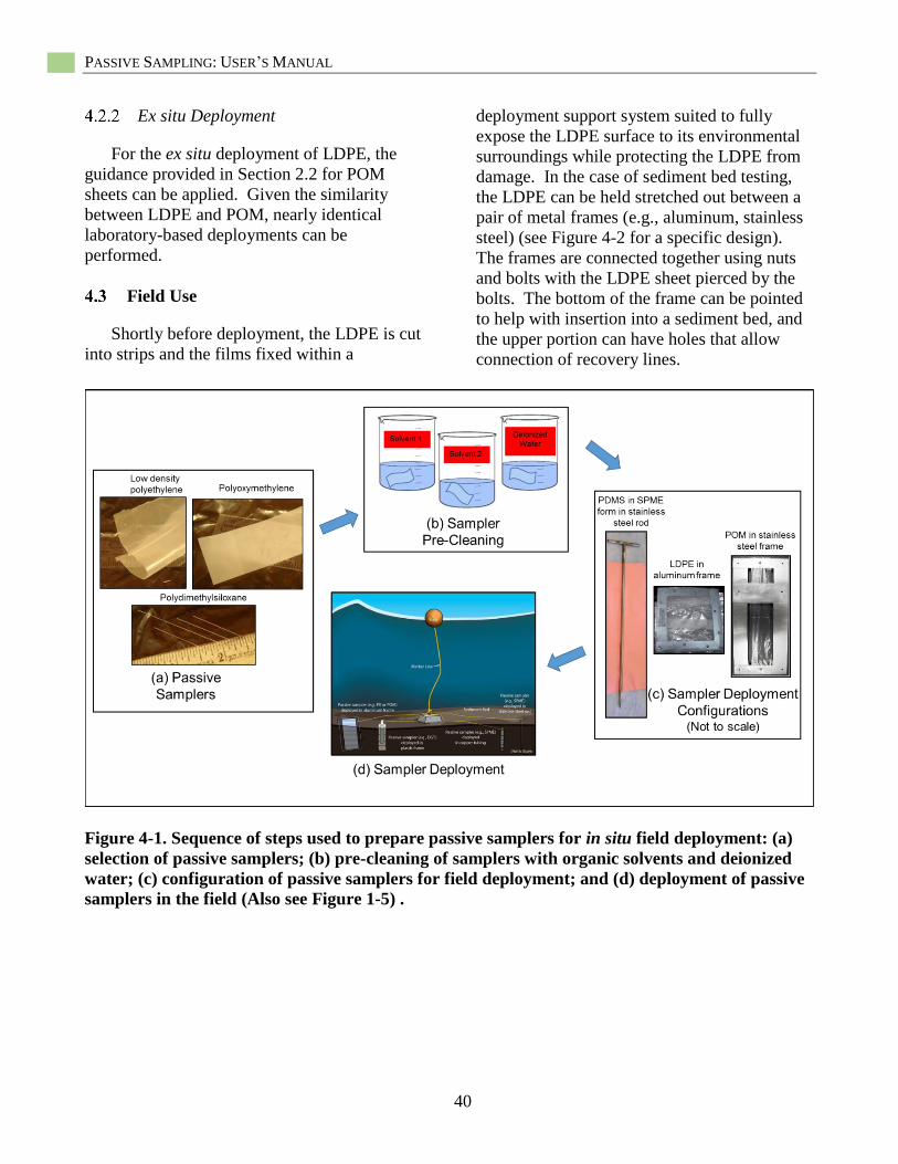
PASSIVE SAMPLING: USER’S MANUAL
40
Ex situ Deployment
For the ex situ deployment of LDPE, the
guidance provided in Section 2.2 for POM
sheets can be applied. Given the similarity
between LDPE and POM, nearly identical
laboratory-based deployments can be
performed.
Field Use
Shortly before deployment, the LDPE is cut
into strips and the films fixed within a
deployment support system suited to fully
expose the LDPE surface to its environmental
surroundings while protecting the LDPE from
damage. In the case of sediment bed testing,
the LDPE can be held stretched out between a
pair of metal frames (e.g., aluminum, stainless
steel) (see Figure 4-2 for a specific design).
The frames are connected together using nuts
and bolts with the LDPE sheet pierced by the
bolts. The bottom of the frame can be pointed
to help with insertion into a sediment bed, and
the upper portion can have holes that allow
connection of recovery lines.
Figure 4-1. Sequence of steps used to prepare passive samplers for in situ field deployment: (a)
selection of passive samplers; (b) pre-cleaning of samplers with organic solvents and deionized
water; (c) configuration of passive samplers for field deployment; and (d) deployment of passive
samplers in the field (Also see Figure 1-5) .

SECTION 4. POLYETHYLENE
41
Figure 4-2. Schematic of a LDPE passive sampling configuration using two aluminum sheet
frames (blue) “sandwiching” a 50 cm strip of LDPE (red) positioned in a “window” for exposure
to the water column and sediments during deployment (drawing by ICF International [Fairfax,
VA, USA]).
If one wants to deploy water-column
samplers during the same field campaign, then
the LDPE can be deployed by placing it inside
a metallic mesh (e.g., aluminum, copper,
stainless steel) (Figure 4-3). The mesh protects
the LDPE from attack by aquatic organisms
(we have observed that ribbons of LDPE
deployed for a month had been chewed on).
The mesh also enables grommets to be used
that enable easy attachment to recovery gear.
After the LDPE is placed in the metal frame
or mesh, the entire assembly is wrapped
carefully and completely in solvent-cleaned,
heavy-duty, metal foil. The wrapped samplers
are also labeled on the outside for field crew
identification, and then they are carefully
arrayed in a clean shipping container (e.g., a
cooler) on ice or ice packs.
For deployment in the field, additional
equipment and lines are used. For example, for
LDPE insertion into relatively shallow
sediments (<5 m), the LDPE frame can be
inserted and locked into a toggle-locking
device (TLD), which is specifically designed
for LDPE installations (Figure 4-4b). The
LDPE is then lowered through the water
column to the surface of the sediment bed and
driven into the sediment so that the LDPE strip
within the frame is positioned across the
sediment-surface water interface. The frame is
then unlocked from the TLD and left in place.
For deployments in moderate depth waters
(e.g., approximately < 20 m), divers can be
used to insert the frames into the bed sediment.
Finally, at still deeper locations, LDPE in the
frame can be affixed to a deployment platform
and the platform lowered from a vessel to the
sediment surface, where the weight of the
platform causes the frame to be inserted into
the sediment bed (Figure 4-4c) (Fernandez et
al. 2014; Fernandez 2009a, b). In addition,
using a hydraulically operated device, the
LDPE sampling frame can be mechanically
pressed into the sediment (Figure 4-4d, Marine
Sampling Systems, Burley WA). In all cases,
recovery lines are attached to the support
frame, and these lines are connected to nearby
pilings, marker surface or subsurface buoys, or
remote releasing devices. As noted in Section
1 (Figure 1-5) in areas where vandalism is a
concern, rather than using surface buoys to
locate passive samplers, lines can be returned
to shore or the use of subsurface buoys may be
considered.

PASSIVE SAMPLING: USER’S MANUAL
42
Figure 4-3. LDPE film deployed inside an aluminum mesh packet.
LDPE is typically left in place for a period
of weeks to months, depending on the target
contaminants of interest. During the
deployment, the target HOCs diffuse into
the LDPE from the surrounding sediments.
As discussed in Section 6, for field (in situ)
deployment of LDPE, the use of performance
reference compounds (PRCs) is highly
recommended. While the target contaminants
accumulate in the sample, the PRCs are
simultaneously diffuse out of the LDPE. Use
of these PRCs is essential, because the rates of
mass transfer of contaminants from the
environment into the LDPE sheets can be
influenced by several environmental factors
(Apell et al., 2015) (e.g., sorption coefficients
of adjacent sediments; turbulence intensity in
adjacent surface water, the uneven formation of
growths, and precipitates that build up on the
LDPE surface) (Figure 4-5).
Recovery and Processing
On recovery from the field exposure,
the LDPE, while still in the frame, should be
cleaned carefully. While the formation of
biofilms and epiphytic growth on LDPE
surfaces does not prevent the polymer from
accumulating target contaminants during
deployment, these coatings can substantially
complicate subsequent chemical analysis
(see Section 7). Careful removal of adhering
sediment or surface growths via water-wetted
laboratory wipes may be necessary. Next, the
LDPE is cut into the appropriate segment
lengths (e.g., to acquire sections exposed to
varying depths in the sediment bed and water
column). The LDPE pieces, usually 10- to
100-mg quantities, are placed in pre-cleaned,
amber glass vials or bottles with a drop of high
purity deionized water for shipping. The water
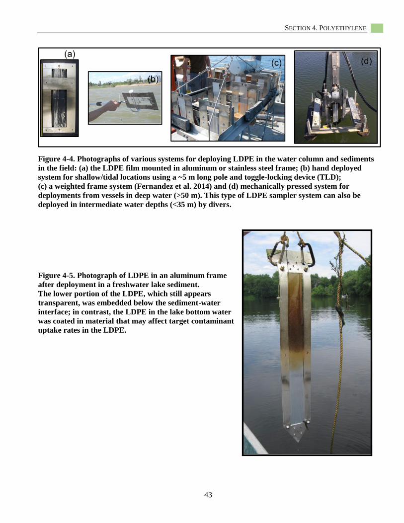
SECTION 4. POLYETHYLENE
43
Figure 4-4. Photographs of various systems for deploying LDPE in the water column and sediments
in the field: (a) the LDPE film mounted in aluminum or stainless steel frame; (b) hand deployed
system for shallow/tidal locations using a ~5 m long pole and toggle-locking device (TLD);
(c) a weighted frame system (Fernandez et al. 2014) and (d) mechanically pressed system for
deployments from vessels in deep water (>50 m). This type of LDPE sampler system can also be
deployed in intermediate water depths (<35 m) by divers.
Figure 4-5. Photograph of LDPE in an aluminum frame
after deployment in a freshwater lake sediment.
The lower portion of the LDPE, which still appears
transparent, was embedded below the sediment-water
interface; in contrast, the LDPE in the lake bottom water
was coated in material that may affect target contaminant
uptake rates in the LDPE.

PASSIVE SAMPLING: USER’S MANUAL
44
is intended to cause the vessel to maintain
100% relative humidity, thereby limiting
sorption of target contaminants to the walls of
the glass vials. Alternatively, the LDPE can be
placed between clean glass or metal plates or
metal foil during transport and sectioned at the
laboratory. Once back at the laboratory, the
samplers are stored at –4°C in the dark unless
extractions can be started by submerging the
PE in organic solvent.
Extraction and Instrumental Analysis
See Section 7.
Data Analysis
See Section 8.
Selection of Published Low-Density
Polyethylene-WaterPartition
Coefficients (KLDPE)
Several researchers have reported LDPE-
water partition coefficients (KLDPE). In all
cases, the partitioning has been described by a
linear isotherm for a wide range of aqueous
concentrations. For this document, partition
coefficients for LDPE are provided for PCBs
and PAHs based on values reported by Ghosh
et al. (2014) and first selected as part of a 2012
Society of Environmental Toxicology and
Chemistry (SETAC) Pellston workshop on
passive sampling (Appendix A). These values
are recommended for use to ensure consistency
across laboratories in the United States using
LDPE to calculate Cfree for PCBs (Table A-1)
and PAHs (Table A-2). Further discussion of
passive sampler partition coefficients is
provided in Appendix B. This discussion
includes alternative partition coefficients for
PCBs and PAHs, as well as other target
contaminants (e.g., selected pesticides, dioxins,
and furans), for which available data sets are
limited and do not allow the designation of
consensus provisional partition coefficients
values at this time.
Along with the listing of partition
coefficients in Appendix A, linear free energy
relationships (LFERs) have been made between
KLDPE (mL water/g LDPE) and KOW to allow
for the calculation of KLDPE for target
contaminants for which empirical partition
coefficients are not available. The following
LFERs relate log KLDPE for PCBs and PAHs
based on Smedes et al. (2009) to log KOW
(Hawker and Connell 1988) for PCBs:
log KLDPE = 1.18 * log KOW – 1.26
(r2 = 0.95) [4-1]
and, similarly, for PAHs, log KLDPE to log KOW
(Hilal et al. 2004):
log KLDPE = 1.22 * log KOW – 1.36
(r2 = 0.99) [4-2]
Alternatively, additional LFERs for LDPE with
PCBs and PAHs are included in Appendix B.
A discussion of the effects of temperature and
salinity on the partitioning of the target
contaminants to polymers can be found in
Appendix C.
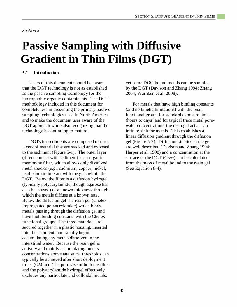
SECTION 5. DIFFUSE GRADIENT IN THIN FILMS
45
Section 5
Passive Sampling with Diffusive
Gradient in Thin Films (DGT) Introduction
Users of this document should be aware
that the DGT technology is not as established
as the passive sampling technology for the
hydrophobic organic contaminants. The DGT
methodology included in this document for
completeness in presenting the primary passive
sampling technologies used in North America
and to make the document user aware of the
DGT approach while also recognizing that the
technology is continuing to mature.
DGTs for sediments are composed of three
layers of material that are stacked and exposed
to the sediment (Figure 5-1). The outer layer
(direct contact with sediment) is an organic
membrane filter, which allows only dissolved
metal species (e.g., cadmium, copper, nickel,
lead, zinc) to interact with the gels within the
DGT. Below the filter is a diffusion hydrogel
(typically polyacrylamide, though agarose has
also been used) of a known thickness, through
which the metals diffuse at a known rate.
Below the diffusion gel is a resin gel (Chelex-
impregnated polyacrylamide) which binds
metals passing through the diffusion gel and
have high binding constants with the Chelex
functional groups. The three materials are
secured together in a plastic housing, inserted
into the sediment, and rapidly begin
accumulating any metals dissolved in the
interstitial water. Because the resin gel is
actively and rapidly accumulating metals,
concentrations above analytical thresholds can
typically be achieved after short deployment
times (<24 hr). The pore size of both the filter
and the polyacrylamide hydrogel effectively
excludes any particulate and colloidal metals,
yet some DOC-bound metals can be sampled
by the DGT (Davison and Zhang 1994; Zhang
2004; Warnken et al. 2008).
For metals that have high binding constants
(and no kinetic limitations) with the resin
functional group, for standard exposure times
(hours to days) and for typical trace metal pore-
water concentrations, the resin gel acts as an
infinite sink for metals. This establishes a
linear diffusion gradient through the diffusion
gel (Figure 5-2). Diffusion kinetics in the gel
are well described (Davison and Zhang 1994;
Harper et al. 1998) and a concentration at the
surface of the DGT (CDGT) can be calculated
from the mass of metal bound to the resin gel
(See Equation 8-4).
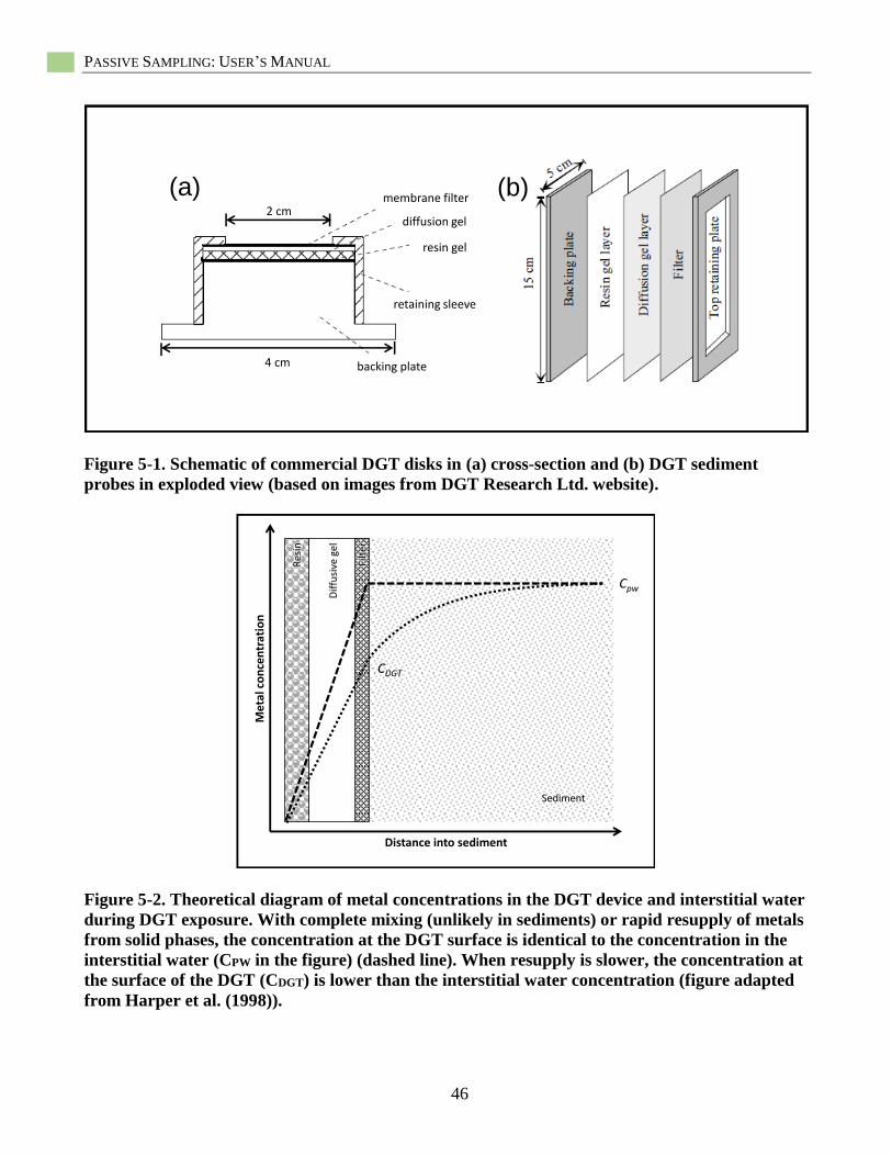
PASSIVE SAMPLING: USER’S MANUAL
46
membrane filter
diffusion gel
resin gel
retaining sleeve
backing plate
(a) (b)2 cm
4 cm
Figure 5-1. Schematic of commercial DGT disks in (a) cross-section and (b) DGT sediment
probes in exploded view (based on images from DGT Research Ltd. website).
Cpw
CDGT
Filt
er
Dif
fusi
ve g
el
Res
in
Sediment
Distance into sediment
Met
al c
on
cen
trat
ion
Figure 5-2. Theoretical diagram of metal concentrations in the DGT device and interstitial water
during DGT exposure. With complete mixing (unlikely in sediments) or rapid resupply of metals
from solid phases, the concentration at the DGT surface is identical to the concentration in the
interstitial water (CPW in the figure) (dashed line). When resupply is slower, the concentration at
the surface of the DGT (CDGT) is lower than the interstitial water concentration (figure adapted
from Harper et al. (1998)).

SECTION 5. DIFFUSE GRADIENT IN THIN FILMS
47
Preparation and Laboratory Use
Unlike POM, PDMS and LDPE which
require some assembly prior to deployment,
DGTs can be purchased as assembled units
from the manufacturer or selected components
can be ordered (e.g., resin gel) (DGT Research
Ltd.) (see Table 1-1) for assembly by the user
in standard or custom-built housings.
Commercially available DGTs for use in
sediments are available in two possible
configurations: a DGT disk (Figure 1-4a) or a
DGT probe (Figure 1-4b). The DGT probe can
be inserted into the sediment vertically to
assess the vertical distribution of metals
(Figure 5-3), and the DGT disk can be placed
on the sediment surface to measure metal flux
to surface waters. Commercially available
DGTs typically have a filter membrane with a
pore size of 0.45 μm, diffusive hydrogel with a
thickness of 0.8 mm, and resin impregnated gel
with a thickness of 0.4 mm.
Prior to use, DGTs should be marked
(probes only) and deoxygenated. DGT probes
should be marked with a fine marker to denote
the location of the sediment/water interface.
The manufacturer recommends placing the
mark ~1–2 cm below the top of the window,
but if the sediment is shallow or compacted, it
may be more appropriate to place the mark
lower. Note that the depth to which the DGT
will accumulate metals is determined by the
distance from the mark to the bottom of the
window. It is recommended that DGTs be
deoxygenated prior to use, which is particularly
important for vertical probes that will likely
interact with anoxic sediments. DGTs can be
deoxygenated for 24 hours in trace metal clean
0.01M NaCl that is gently bubbled with N2 or
Ar gas.
Figure 5-3. Photograph of the ex situ
deployment of DGT samplers in simulated
water column – whole sediment system
(image provided by S Simpson [CSIRO,
Sydney, Australia]).
Field Use
DGTs have been used effectively in situ for
both water column and sediment assessments
of labile (e.g., Costello et al. 2012). DGTs
should be used soon after deoxygenating, to
minimize the introduction of oxygen into the
sediment by DGT placement. DGTs are
transported in sealed plastic bags in a cooler to
the field site and deployed within 24 hrs. DGT
disks are used by pressing the assembly gently
onto the surface of the sediment. Disk
assemblies are slightly negatively buoyant and
will maintain contact with the sediment under
static conditions. However, in flowing waters,
it is necessary to weigh down the DGT disks or
use the DGT probe assembly. The DGT probe
assembly is inserted into the sediment
vertically, with a smooth motion, until the
marked line is at the sediment/water interface.
PASSIVE SAMPLING: USER’S MANUAL
48
Be sure to note the time of DGT
deployment and the temperature of the
sediment (i.e., temperature is a variable in
calculating the diffusion coefficient (D)). The
DGT deployment time should be sufficiently
long to accumulate a measureable quantity of
metal on the resin but short enough to avoid
depleting the supply of metal in the interstitial
water (see below). In some cases, retrieval of
replicate DGTs at different time points can
yield useful information about metal dynamics.
For single retrieval, a deployment time of
~24 hours has been used successfully and is
recommended.
For sediment assessments, it is
recommended that the vertical DGTs (with
15-cm by 1.8-cm exposure windows) be used
and gently inserted approximately 10 cm into
the sediment. The depth of penetration should
be measured and then rechecked at retrieval.
This approach allows for determination of the
differences in labile metals associated with
deep and surficial sediments, and also the
overlying waters. If DGTs are deployed
repetitively through time, then temporal
changes also can be assessed (Costello et al.
2012). As noted in Section 1 (Figure 1-5), in
areas where vandalism is a concern, rather than
using surface buoys to locate passive samples,
lines can be returned to shore or the use of
subsurface buoys may be considered.
Recovery and Processing
After deployment, the DGTs are removed
from the sediment and stored until processing.
DGTs are removed gently from the sediment,
and any adhering sediment particles are washed
off with deionized water. If processing is not
performed immediately (e.g., field-deployed
DGTs), the DGT apparatus can be stored in a
clean plastic bag and refrigerated.
For DGT disks, the plastic housing is
removed by placing a flat-head screwdriver in
the slot and twisting until the outer housing
pops off. Without disassembling the probe, the
filter and gels can be cut along the edges of the
DGT housing window using a Teflon-coated
razor. It is important to cut entirely through to
the bottom of the gels, because the resin gel can
easily deform. The entire gel and filter section
is removed from the housing using plastic
forceps and placed on an acid-cleaned Perspex
or Lucite plate (i.e., polymethyl methacrylate
(PMMA)). The membrane filter and diffusive
gel are removed carefully and discarded. Using
the Teflon-coated razor blade, carefully cut
measured sections of the resin gel
corresponding to the appropriate sediment
depth. Sections can range from 1 to 20 mm,
depending on the resolution required.
Extraction and Instrumental Analysis
See Section 7.
Data Analysis
See Section 8.
SECTION 6. PERFORMANCE REFERENCE COMPOUNDS
49
Section 6
Selection and Use of Performance
Reference Compounds for
Hydrophobic Organic Target
Contaminants Introduction
While many passive samplers used with
hydrophobic organic contaminants have been
shown to reach equilibrium with sediment in
well-mixed slurry systems within a month, the
time necessary to reach equilibrium under
field-deployed (i.e., in situ) conditions is slow.
Performance reference compounds (PRCs) can
be used to estimate the extent of equilibrium of
the target contaminant(s) and provide a method
to then adjust measured accumulated target
contaminant levels to equilibrium
concentrations. In passive sampler
deployments where the demonstration of target
contaminant equilibrium with the passive
sampler is not determined directly using
temporal sampling or different polymer
thicknesses, PRCs can be used. One clear
benefit of using PRCs is that they take into
consideration the effects on attaining
equilibrium of biofilm growth and fouling on
the passive sampler surface. Consequently, it is
highly recommended that PRCs be applied to
passive sampling deployments whenever
possible. PRCs are chemicals that behave like
the target contaminants and are loaded into
the passive sampler polymer prior to the
deployment (Huckins et al. 2002). A good
PRC should (i) allow precise measurement
of its loss, (ii) follow similar same kinetics
bracketing the target analyte, and (iii) not occur
in the environment (Fernandez et al. 2009a;
Huckins et al. 2002). Performance reference
compounds have been used with LDPE and
POM and less often than with PDMS-based
systems. Because of the very small mass of
PDMS associated with the SPME fiber, target
contaminants are often considered to achieve
equilibrium with it relatively rapidly compared
to LDPE and POM. This PRC-free approach
with PDMS has been explored in in situ
deployments (e.g., Witt et al. 2013; Maruya
et al. 2015) and is worth further careful
investigation because of the time and cost
savings (e.g., no need to use PRCs) that could
be gained in some in situ passive sampler
applications. However, it is critical that target
contaminant equilibrium is demonstrated
before this PRC-free approach is used in situ
otherwise Cfree may be underestimated resulting
in an underestimation of exposure. PRCs are
not used with DGT passive sampling and risk.
Using Performance Reference
Compounds (PRCs)
Selecting PRCs
It is very important to avoid adding PRCs
to the passive sampler that the analytical
laboratory is using as surrogate (i.e., recovery)
or injection standard (see Section 7). One
subset of compounds should be used as PRCs,
while reserving others for use as surrogate
(recovery) compounds. Still other compounds
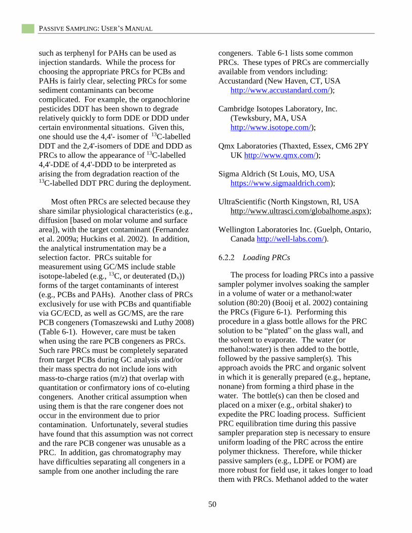
PASSIVE SAMPLING: USER’S MANUAL
50
such as terphenyl for PAHs can be used as
injection standards. While the process for
choosing the appropriate PRCs for PCBs and
PAHs is fairly clear, selecting PRCs for some
sediment contaminants can become
complicated. For example, the organochlorine
pesticides DDT has been shown to degrade
relatively quickly to form DDE or DDD under
certain environmental situations. Given this,
one should use the 4,4'- isomer of 13C-labelled
DDT and the 2,4'-isomers of DDE and DDD as
PRCs to allow the appearance of 13C-labelled
4,4'-DDE of 4,4'-DDD to be interpreted as
arising the from degradation reaction of the 13C-labelled DDT PRC during the deployment.
Most often PRCs are selected because they
share similar physiological characteristics (e.g.,
diffusion [based on molar volume and surface
area]), with the target contaminant (Fernandez
et al. 2009a; Huckins et al. 2002). In addition,
the analytical instrumentation may be a
selection factor. PRCs suitable for
measurement using GC/MS include stable
isotope-labeled (e.g., 13C, or deuterated (Dx))
forms of the target contaminants of interest
(e.g., PCBs and PAHs). Another class of PRCs
exclusively for use with PCBs and quantifiable
via GC/ECD, as well as GC/MS, are the rare
PCB congeners (Tomaszewski and Luthy 2008)
(Table 6-1). However, care must be taken
when using the rare PCB congeners as PRCs.
Such rare PRCs must be completely separated
from target PCBs during GC analysis and/or
their mass spectra do not include ions with
mass-to-charge ratios (m/z) that overlap with
quantitation or confirmatory ions of co-eluting
congeners. Another critical assumption when
using them is that the rare congener does not
occur in the environment due to prior
contamination. Unfortunately, several studies
have found that this assumption was not correct
and the rare PCB congener was unusable as a
PRC. In addition, gas chromatography may
have difficulties separating all congeners in a
sample from one another including the rare
congeners. Table 6-1 lists some common
PRCs. These types of PRCs are commercially
available from vendors including:
Accustandard (New Haven, CT, USA
http://www.accustandard.com/);
Cambridge Isotopes Laboratory, Inc.
(Tewksbury, MA, USA
http://www.isotope.com/);
Qmx Laboratories (Thaxted, Essex, CM6 2PY
UK http://www.qmx.com/);
Sigma Aldrich (St Louis, MO, USA
https://www.sigmaaldrich.com);
UltraScientific (North Kingstown, RI, USA
http://www.ultrasci.com/globalhome.aspx);
Wellington Laboratories Inc. (Guelph, Ontario,
Canada http://well-labs.com/).
Loading PRCs
The process for loading PRCs into a passive
sampler polymer involves soaking the sampler
in a volume of water or a methanol:water
solution (80:20) (Booij et al. 2002) containing
the PRCs (Figure 6-1). Performing this
procedure in a glass bottle allows for the PRC
solution to be “plated” on the glass wall, and
the solvent to evaporate. The water (or
methanol:water) is then added to the bottle,
followed by the passive sampler(s). This
approach avoids the PRC and organic solvent
in which it is generally prepared (e.g., heptane,
nonane) from forming a third phase in the
water. The bottle(s) can then be closed and
placed on a mixer (e.g., orbital shaker) to
expedite the PRC loading process. Sufficient
PRC equilibration time during this passive
sampler preparation step is necessary to ensure
uniform loading of the PRC across the entire
polymer thickness. Therefore, while thicker
passive samplers (e.g., LDPE or POM) are
more robust for field use, it takes longer to load
them with PRCs. Methanol added to the water
SECTION 6. PERFORMANCE REFERENCE COMPOUNDS
51
(e.g., 80:20 methanol:water) swells the passive
sampler polymer to some extent, and
equilibration takes somewhat less time than the
water-only solutions (Booij et al. 2002).
Loading with PRCs using methanol:water has
been applied with all three types of samplers
(e.g., Perron et al. 2013a, 2013b, Thomas et al.
2014). However, such loading requires soaking
the passive sampler in water to remove
methanol after the PRC addition. If the PRCs
were loaded from methanol:water solution, just
before deployment, the PRC-loaded passive
sampler is rinsed with high quality water, and
then it is soaked in high quality water for 24
hours to remove methanol from the polymer.
This methanol removal step is repeated twice to
ensure complete methanol removal.
Equilibration times also vary for different
PRC/passive sampler thickness combinations
and the passive sampler to water phase ratio.
For PAHs and PCBs in aqueous solution, at
least a 30-day duration is needed to ensure
homogeneous distributions of the PRCs
throughout the entire thickness of the LDPE
film, unless faster equilibration has been
confirmed. Equilibration times from
methanol:water solutions are typically
completed within seven days (Booij et al.
2002). Confirmation of PRC loading
equilibration can be performed by time course
measures of PRC concentrations in the polymer
or by showing that concentrations of PRCs are
the same for films of different thicknesses but
the same masses. Once loaded with PRCs the
samplers generally are stored in the PRC
solution until shortly before deployment. It is
critical to retain at least one (i.e., replicates are
recommended) sample of PRC that is loaded in
a passive sampler but not deployed. This
passive sampler will be analyzed to determine
the initial PRC concentrations in the polymer
(PRCi) for later analysis. Ideally, replication of
the undeployed passive sampler would match
the replication used in the deployment design.
For example, if three passive samplers were
deployed at each field station, or three replicate
chambers were used in the laboratory, then
unique pieces of three passive sampler
polymers would be prepared to determine
PRCi.
While the medium and high KOW PRCs are
relatively stable once accumulated by the
passive sampler polymer, low KOW PRCs may
start to exit the polymer via volatilization once
they are removed from the PRC-loading
solution. If the purpose of a deployment is
focused on low KOW target contaminants
(e.g., naphthalene) using low KOW PRCs, it is
advisable to analyze sub-samples of the
samplers to determine how much PRC has been
lost prior to deployment.
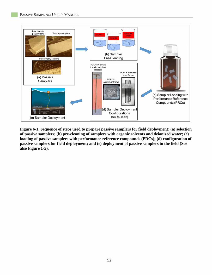
PASSIVE SAMPLING: USER’S MANUAL
52
Figure 6-1. Sequence of steps used to prepare passive samplers for field deployment: (a) selection
of passive samplers; (b) pre-cleaning of samplers with organic solvents and deionized water; (c)
loading of passive samplers with performance reference compounds (PRCs); (d) configuration of
passive samplers for field deployment; and (e) deployment of passive samplers in the field (See
also Figure 1-5).

SECTION 6. PERFORMANCE REFERENCE COMPOUNDS
53
Table 6-1. Examplea performance reference compounds (PRCs), as well as surrogate standards
(internal standards), and injection standards for different classes of contaminants when using
low density polyethylene (LDPE) passive samplers.
Target Contaminant
Performance
Reference Compounds
(PRCs)
Surrogates/Internal
Standards Injection Standards
Polycyclic aromatic
hydrocarbons (PAHs)
D10-phenanthrene
D10-pyrene
D12-chrysene
D10-anthracene
D10-fluoranthene
D12-benz(a)anthracene
D10-acenaphthene
D14-m-terphenyl
D12-perylene
Polychlorinated biphenyls
(PCBs)
13C12 CB-28 13C12 CB-52 13C12 CB-101 13C12 CB-153 13C12 CB-180
13C12 CB-19
D6 CB-77
D5 CB-116
CB-198 13C12 CB-105 13C12 CB-167 13C12 CB-170 13C12 CB-194
D6 CB-77
D5 CB-116
DDTs 2,4’-DDD
2,4'-DDE 13C12 2,4'-DDD 13C12 4,4'-DDT
CB-111 13C12 CB-153 13C12 2,4'-DDT
D6 CB-77 13C12 CB-105 13C12 CB-167
a This example assumes that gas chromatography/mass spectroscopy is the analysis method with
detection limits of approximately 100 – 200 pg/100 mg LDPE.
Determining the Quantity of PRC to
Load into Passive Samplers
To determine how much PRC should be
loaded into a passive sampler for laboratory
(ex situ) or field deployments (in situ), one
should first estimate the expected concentration
of the target contaminants in the sampler post-
deployment. This estimate can be based on
historical water or sediment interstitial water
data or modeling interstitial water
concentrations using equilibrium partitioning
and measured sediment target contaminant
concentrations. Following deployment, target
contaminants and PRCs should have
comparable concentrations, so that if dilution or
further extract concentrating is necessary for
analytical reasons, quantification of both the
targets and PRCs is possible in the same
analysis. Also, it is important to ensure that
depleted PRC concentrations will be
quantifiable, given the sampler size and final
extract concentrations. For example, if PRCs
are loaded at 0.50 µg/g to a one gram passive
sampler, it is important to make certain, given
instrument detection limits, that it is possible
to quantify 0.05 µg/g (i.e., ~50 ng/mL for 1 mL
final extract volume, or ~25 ng/mL for a
0.5 g-sampler in a one milliliter final extract
volume), in the event that 90% of a given PRC
is depleted. In this instance, if concentrations
of the target contaminants are on the order of
50 µg/g, it may be difficult to accurately
quantify the loss of the PRCs and use them to
adjust for equilibrium concentrations of target
contaminants.
Once the loaded PRC concentration in the
passive samplers and the number of samplers
to be loaded have been determined, a loading or
spiking solution volume and concentration can
be calculated. First, determine the volume of

PASSIVE SAMPLING: USER’S MANUAL
54
loading solution that is needed. Note that
exceeding a 0.03 g polymer/mL loading
solution ratio can result in problems with
physically getting all of the polymer into the
loading solution. Once the mass of PE and
volume of loading solution have been
determined, then the concentration necessary
to load into the samplers can be estimated.
First, determine the equilibrium concentration
of each PRC in the loading solution, based on
that PRC’s concentration as needed in the
passive sampler using the same partitioning
approach applied to determine Cfree from CPS
(based on Equation 1-3). The total amount of
PRC needed can be determined by summing
the mass of PRC in both the passive sampler
polymer and the loading solution at
equilibrium. To calculate the mass in the
polymer, divide the equilibrium concentration
by the total mass of polymers to be pre-loaded,
and to calculate total mass in the loading
solution, divide the solution's concentration by
the total volume. If loading with a
methanol/water solution (as opposed to just
water), methanol:water partitioning coefficients
(KMS) for LDPE and PDMS are given by Booij
et al. (2002). To estimate KMS for compounds
not measured by Booij et al. (2002), an
estimation can be performed by correlating the
log KOW to the log KMS given in the same
publication. Note that KMS is not presented as
a log value (Booij et al. 2002), and the units are
mL/g.
To load the PRCs into the sampler, first
prepare the loaded PRC solution. Make sure
that the container in which you intend to load
the samplers is sufficiently large for both the
samplers and the loading solution. Once the
PRC solution is ready, add the samplers one at
a time, eliminate air bubbles on the polymers,
and maximize the sampler solvent contact until
all samplers are submerged in the loading
solution. If there is a significant amount of
headspace in the container, consider adding
more solvent (i.e., water or methanol:water) —
although this will lower your spiking
concentrations somewhat. Seal the container
with a watertight, ground glass stoppered lid,
and protect the solution from light (either in
amber glass or cover with foil). To accelerate
the loading process, place the container on an
orbital shaker to agitate the loading solution
and enhance transfer of PRCs into the passive
sampler polymer. Generally, the loading
period will be at least as long as the
deployment period. As noted, if using the
methanol:water solution to load the passive
samplers, this solution causes the polymer
matrix to expand, allowing faster loading, and
the process will take less time than using a high
quality water loading solution. However, one
must plan on a day or two to leach methanol
from the passive sampler before deployment.
Once the loading process is complete, the
samplers can be left in the loading solution (for
water) or the leaching solution (for methanol-
water) in the dark until the laboratory or field
deployment. The time necessary to load the
PRCs into a passive sampling polymer such
that they reach equilibrium can be estimated
using diffusion modeling but requires some
sophistication and acquiring assistance from
one of the technical contacts listed in Table 1-4
is highly recommended.
Example Calculation
The following example describes (i) how
much PRC to load into a given passive sampler,
(ii) the amount of PRCs to add to the batch of
samplers being deployed together, and (iii) the
loading solution volume and concentrations of
PRCs. The example assumes that the loading
solution is pure water and not a solution
containing a mixture of water and methanol.
To load passive sampler polymers with PRCs
in a water:methanol solution, see the
methodology discussed in Booij et al. (2002).
In this simple example, based on
equilibrium partitioning modeling, interstitial
waters at a contaminated sediment site are

SECTION 6. PERFORMANCE REFERENCE COMPOUNDS
55
expected to have concentrations of PCB
congener 52 (CB52) at about 10 ng/L
interstitial water. Rearranging Equation 1-3,
we can estimate the concentration of CB52 that
would accumulate in a one kilogram LDPE:
freeLDPELDPE CKC * [6-1]
where, the KLDPE for CB52 is 354813 L/kg
LDPE (Appendix A), and Cfree is set equivalent
to an equilibrium partition based estimate of
10 ng/L for the interstitial water concentration.
In this case, CLDPE is 3.55106 ng/kg LDPE,
or 3.55 µg/g LDPE. Given this result, the
samplers will be loaded with 3.55 µg/g LDPE
using the PRC 13C CB52 (i.e., the best PRC
for CB52). If during the deployment, the PRC
is depleted by 90%, there would still be
0.355 µg/g LDPE in the sampler, which is well
above the equivalent instrumental detection
limit for CB52 using GC/MS (i.e., for this
example, 3550 ng/mL versus the detection limit
of 50 ng/mL) using a LDPE density of
0.92 g/mL.
Next, the loading solution will be 2000 mL
for 50 g of LDPE samplers (n = 50 individual
passive samplers are to be deployed). Again
using Equation 1-3, modified for LDPE, the
sampler loading solution concentrations can
be determined:
LDPE
LDPEfree
K
CC [6-2]
Now, Cfree is set equal to the loading solution
concentration of the PRC 13C CB52, and CLDPE
is the 3.55 µg of PRC 13C CB52 /g LDPE
calculated above. Here, the loading solution
concentration is determined to be 10 µg/L
loading solution. Given the results of this
calculation and the volume of loading solution
(2000 mL), 197.5 µg of PRC 13C CB52 will be
needed for preparing the loading solution. One
vendor, Cambridge Isotope Laboratories, Inc.,
offers 13C CB52 in 40 µg/mL organic solvent
units of 1.2 mL or 3.0 mL which can be used to
prepare the loading solution. For this example,
5 mL of the venders 13C CB52 is required to
prepare the loading solution.
Chemical Analysis of PRCs following
Deployment
Following recovery of the passive samplers,
instrumental chemical analysis of the PRCs is
performed as part of the analysis of the target
contaminants (see Section 7). During the data
analysis (Section 8), the post-deployment
concentrations of the PRCs are determined
(CPRC(f)). In addition, the sample from the non-
deployed passive sampler is also analyzed to
determine the initial concentration of PRCs
(CPRC(i)) in the passive samplers. These two
values are used to calculate the measured
fraction of each PRC (fmeqPRCx) lost from the
sampler section during its deployment (see
Equation 8-3). As noted above, analyses would
be performed in an effort to match the
replication used in the field or laboratory
deployments.
PASSIVE SAMPLING: USER’S MANUAL
56
Section 7
Extraction and Instrumental Analysis
of Target Contaminants from Passive
Sampling Introduction
Following deployment and storage of the
passive samplers, chemical analysis is the next
step in their processing. This part of the
process is addressed in two steps in this
section: first, the extraction of target organic
contaminants and metals from the passive
sampler polymer, and second, the actual
instrumental chemical analysis of the resulting
extracts (Table 7-1). Neither of these exercises
is overly difficult. For example, extraction of
the passive samplers is, in most cases, simpler
than extracting sediments, soils, or tissues.
However, the extraction procedures are not yet
commonly performed in commercial
laboratories, so they will be descibed here in
detail (Figure 7-1).
Ideally, the POM and LDPE passive
samplers deployed in situ will arrive
refrigerated at the analytical laboratory in glass
jars generally in coolers. The size of the jars
will depend on the objectives of the
investigation but will likely range from 20 mL
to four liters in volume. The PDMS passive
samplers deployed in situ, in the form of SPME
fibers, will also arrive at the analytical
laboratory in glass jars refrigerated but because
of the SPME’s small size, the jars will most
often range in volume from 2 to 20 mL. For
POM, LDPE and PDMS, the storage/transport
jars should use clean foil as a lid liner (not a
plastic polymer [e.g., Teflon]). The POM and
LDPE films and SPME fibers can be processed
in the field by the addition of organic solvent to
the glass jars holding the retrieved passive
samplers. This initiates the extraction and
reduces the loss of volatile target contaminants
during transport and storage. It is extremely
critical to confirm that vials and jars are firmly
sealed and that solvent will not leak during
transport. If the samplers require extensive
cleaning at the laboratory, they should not have
solvent added to them in the field. In addition,
if the passive sampler cannot be processed in
the field or upon arrival at the laboratory
(which is recommended), they should be stored
at or below 4.0 ˚C in the dark until processing
can be started.
After recovery, the DGT samplers should
be rinsed with deionized water prior to
placement in a clean plastic bag. A few drops
of deionized water is added to the interior of
the bag to maintain moist conditions and
prevent drying. When the DGT samplers arrive
at the analytical laboratory they should be
refrigerated (~4.0 ˚C) in the dark in the same
plastic bag (but not frozen).
Regarding the instrumental chemical
analysis, once extracted and reduced to an
organic solvent extract for organic target
contaminants, or an acid extract for target metal
contaminants, the chemical analysis is identical
precedurally and cost-wise to a water,
sediment, soil, or tissue analysis. In fact, the
passive sampler extracts may be easier to
analyze because the polymers generally don’t
SECTION 7. EXTRACTION AND INSTRUMENTAL ANALYSIS
57
require the degree of clean-up needed by
sediment, soil, and tissue extracts. For organic
target contaminants, one difference from
conventional extracts and analyses, as
discussed in Section 6, is that the passive
sampler extracts may contain performance
reference compounds that will need to be added
to the analyte list of the analytical instrumental
method.
Further, as with the rest of this document,
the target contaminants consists of the
conventional legacy pollutants, including the
hydrophobic organic contaminants,
polychlorinated biphenyls (PCBs) and
polycylic aromatic hydrocarbons (PAHs),
and metals (e.g., cadmium, copper, nickel, lead,
zinc). In part, this is because the extraction
and analytical methods have been developed
and standardized for these contaminants, and
these methods can be revised easily for use
with passive samplers. Further, these are the
classes of contaminants that occur at many
contaminated sites around the country and
drive monitoring and remediation efforts.
As noted earlier, for organic target
contaminants, other classes of contaminants
can be measured with the assistance of passive
sampling, including chlorinated pesticides such
as DDT and its degradation products and the
chlorinated dioxins and furans. However, data
needed for the passive sampling of these target
contaminants, like partition coefficients and
analytical methods, are not readily available
at present. This is not to suggest that methods
for other classes of contaminants, including
contaminants of emerging concern, are not
available for use with passive samplers (e.g.,
Perron et al. 2013b). However, in many cases,
greater method development would likely be
needed, because standardized methods may
not have been fully established.
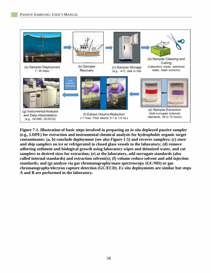
PASSIVE SAMPLING: USER’S MANUAL
58
Figure 7-1. Illustration of basic steps involved in preparing an in situ deployed passive sampler
(e.g., LDPE) for extraction and instrumental chemical analysis for hydrophobic organic target
contaminants: (a, b) conclude deployment (see also Figure 1-5) and recover samplers; (c) store
and ship samplers on ice or refrigerated in closed glass vessels to the laboratory; (d) remove
adhering sediment and biological growth using laboratory wipes and deionized water, and cut
samplers to desired sizes for extraction; (e) at the laboratory, add surrogate standards (also
called internal standards) and extraction solvent(s); (f) volume reduce solvent and add injection
standards; and (g) analyze via gas chromatography/mass spectroscopy (GC/MS) or gas
chromatography/electron capture detection (GC/ECD). Ex situ deployments are similar but steps
A and B are performed in the laboratory.

SECTION 7. EXTRACTION AND INSTRUMENTAL ANALYSIS
59
Table 7-1. Summary of extraction and analytical methods for passive samplers discusssed in this
section including U.S. EPA methods for analyzing PCBs, PAHs, and metals, as well as other
selected contaminant classes.
Target
Contaminant
Passive
Sampler Extraction
Contaminant
Class Analytical Methods
Hydrophobic
Organic
Contaminants
POM,
PDMS,
LDPE
Organic
solvents
(acetone,
hexane,
acetonitrile,
methylene
chloride)
Polycyclic
aromatic
hydrocarbons
Method 8310: HPLC
Method 8270D or 8270-Selecting
Ion Monitoring: SVOCs by GC/MS
Polychlorinated
biphenyls
Method 8082A: GC/ECD or
GC/ECD
Method 1668c: HRGC/HRMS
Method 8270-Selected Ion
Monitoring: GC/MS
Chlorinated
pesticides
Method 1699: Pesticides by
HRGC/HRMS
Method 8081B: Organochlorine
pesticides by GC
Method 8270D or 8270-Selected Ion
Monitoring: SVOCs by GC/MS
Polychlorinated
dibenzodioxins/
Polychlorinated
dibenzofurans
Method 8280B: HRGC/LRMS
Method 8290A: HRGC/HRMS
Method 1613B: HRGC/HRMS
Metals DGT Inorganic
acids (Nitric
acid)
Cadmium,
copper, nickel,
lead, zinc
Method 6020A (also APHA Method
3125): ICP-MS
PASSIVE SAMPLING: USER’S MANUAL
60
Extraction for POM, PDMS, and
LDPE
The general extraction procedure is
basically the same for each type of passive
sampler discussed in this document. Once
received by the analytical laboratory, each type
of passive sampler is amended with surrogate
standards (also called internal standards)
chosen to complement the target contaminants
of interest to assess target analyte recoveries
(see Table 6.1). Subsequently, the samplers are
each submerged in a suitable solvent
(e.g., methylene chloride) for at least 12 hours.
A shaker table or some other suitable
mechanical agitation is recommended for the
extractions, to facilitate sampler-solvent contact
and target contaminant transport. The extract is
transferred to a large vessel suited for solvent
evaporation, and then the sampler is re-
extracted two more times with organic solvent,
with the extracts combined for evaporative
volume reduction, and eventual gas
chromatography/mass spectroscopy (GC/MS)
(or suitable) instrumental analysis. After the
extraction, the sampler is air-dried and
weighed. Before analysis, appropriate injection
standards are added to the final extracts to
allow for evaluation of the injection efficiency.
For strongly hydrophobic and low volatility
target contaminants, there will be limited loss
from polymers even if processing is conducted
after shipment to a laboratory. For low
hydrophobicity, volatile target contaminants,
however, immediate processing may be
necessary to minimize the losses. Volatile
compounds such as naphthalene or similar
should be processed rapidly in the field (i.e.,
transferred to a vial containing organic solvent)
and tested for volatile losses from the thickness
and sorbent employed. For example,
substantial volatilization of naphthalene from
30 μm thick PDMS exposed directly to the air
occurs on the order of minutes (Reible and
Lotufo 2012). Retention is maximized by
using a thicker polymer or polymer with a
greater affinity for the target contaminant or by
focusing on less volatile target contaminants.
Evaporative losses can also be minimized by
placing samplers in a sealed bag and cooling
for shipment to the laboratory. For example,
phenanthrene losses from 30 µm PDMS were
negligible over 24 hours when prepared in this
manner (Reible and Lotufo 2012). Adding a
small volume of deionzied water will also limit
volatilization.
The affinity for many target contaminants
to the extraction solvents such as hexane,
methanol, or acetonitrile is equal to or stronger
than that of the polymers, and thus, extraction
is complete as long as the volume of extraction
solvent is much greater than the volume of
polymer. For example, typically less than
1–10 µL of PDMS sorbent is employed in a
sample, so extraction with 10–100 µL of
solvent is sufficient to insure essentially
complete extraction.
7.2.1 Extraction of POM
Text Box 7.2 provides a detailed
description of the steps involved for the
extraction of POM for PCBs and PAHs.
7.2.2 Extraction of PDMS
Text Box 7.1 provides a detailed
description of the steps involved for the
extraction of PDMS for PCBs and PAHs.
For this description, the PDMS is assumed to
be associated with an SPME fiber, rather than
in a sheet configuration. If the PDMS is
deployed in a sheet configuration, the polymer
will be extracted in a similar way as POM and
LDPE.
SECTION 7. EXTRACTION AND INSTRUMENTAL ANALYSIS
61
Text Box 7-1. Outline of example procedures for extracting PAHs and PCBs from POM.
Extraction Procedure
Preliminary: After field or laboratory deployment, carefully remove sampler polymer from
any deployment gear and clean by wiping with laboratory wipes
1. The POM film is inspected for surface biofilms, particles, mud, oily coatings, and other residues.
Biofilm mass should be removed using a clean wipe followed by a rinse with deionized water.
Sedimentary debris is removed by rinsing with deionized water and careful surface scraping with a
razor if necessary to remove adhered/embedded material. Oily coatings (e.g., hydrocarbon slicks)
are removed by soaking clean wipes in hexane and using forceps to wipe both POM surfaces. This is
a rapid and non-exhaustive rinsing performed immediately prior to immersion in organic solvent for
the actual extraction. To limit the presence of water, POM surfaces are blotted dry if necessary.
2. To start the extraction, use clean, labeled, glass vials, one for each POM strip. The size of the
polymer strips will vary depending on the expected concentration of target contaminants. For
example, samplers exposed to sediment interstitial water will be smaller than samplers deployed in
the water column. Add sufficient acetone/hexane (1:1 by volume) to each vial to completely
submerge the POM strips. Use pesticide residue–grade solvents.
3. Add surrogate solution to each extraction vial (e.g., 30 µl of 500 µg/L of selected PCB congeners
and PAH molecules added to 40 mL vial). Surrogate standard is also called internal standard. It is
critical to avoid using surrogate (internal) and injection standards that may co-elute or interfere with
performance reference compounds (PRCs) as discussed in Section 6.
4. Transfer each POM strip to one of the vials. Tightly cap the vials using Teflon-line caps.
5. Place POM extraction vials on an orbital shaker running at 30 rpm. Cover or use amber vials to
prevent photo-degradation of light sensitive target contaminants. Note the time.
6. After a 24-hour extraction period, remove the vials from the shaker.
7. Prepare clean, labeled glass vials with a capacity approximately three times that of the extraction
vials, one for each POM strip. From each of the extraction vials, transfer the solvent extract, but not
the POM strip, to its corresponding large capacity vial. Cap, wrap (to reduce photodegradation), and
freeze the vials.
8. Add fresh acetone/hexane (1:1 by volume) to each of the extraction vials still containing the POM
strips. Cap, wrap, cover to prevent photodegradation, and place on the shaker for another 24 hours.
9. After the second 24-hour extraction, transfer the liquid extract of each strip to the corresponding
large capacity vial containing the first day’s extract (i.e., combine the first and second extracts of
each strip). Cap, wrap, and freeze the large capacity vials.
10. Perform the third and final extraction by repeating steps 7 and 8.
11. Allow the extracted POM strips to dry, and record their weights using an analytical balance. This
result is used to calculate the final target contaminant concentrations measured in the POM sampler
in units of contaminant mass per POM mass (e.g., ng/g POM).
12. Using rotary evaporation or equivalent volume reduction equipment, reduce the final extracts in the
large capacity vials and proceed with sample clean-up (if necessary) and instrumental analysis for
selected PCB congeners and PAHs. The final volume will depend on the specific laboratory
procedures: 1 to 2 mL is recommended.

PASSIVE SAMPLING: USER’S MANUAL
62
Extraction Procedure
13. The solvent extracts are stored at -4°C in the dark until ready for instrumental analysis.
14. Before analysis, appropriate injection standards are added to the final extracts to allow for evaluation
of losses during the injection and instrumental analysis (Table 6-1).
Text Box 7-2. Outline of example procedures for extracting PAHs and PCBs from PDMS.
Extraction Procedures
Preliminary: The following description is for a modified push point sampler used in a field
deployment applying SPME fibers (not PDMS sheets). However, the basic procedures are
applicable to laboratory deployed PDMS samplers or field deployed PDMS samplers using
configurations other than the push point sampler
1. After removal from the field, the sampling device’s inner rod is separated from the outer sheath. The
SPME PDMS fiber is carefully removed from the inner rod using a single-edge razor, and adhering
sediment, particles, biofilm, and any residue is removed from the SPME PDMS fiber using
deionized water-wetted laboratory wipes. SPME PDMS fibers are then blotted dry before
segmentation.
2. Laboratory and/or field blank and field-deployed SPME PDMS fibers are segmented, using a
ceramic column cutter into predetermined lengths at points along the SPME PDMS fiber, which
correspond to specific depths of interest from the sediment-water interface.
3. The SPME PDMS fiber segments are transferred to 2-mL glass amber vials (i.e., auto-sampler vials)
that contain a 300-μL glass vial insert. The inserts should be prefilled with the appropriate solvent
(e.g., acetonitrile for PAHs, hexane for PCBs). The solvent volume should be sufficient for the
complete immersion of the SPME PDMS fiber segment. Add surrogate standard to each 300 µL
glass vial insert.
4. The SPME PDMS fiber segments are left in the solvent for 12 to 24 hours and stored at –17°C until
analysis. During transportation, the samples are kept at a temperature not to exceed 4°C.
5. The SPME PDMS fiber segments are removed from the solvent before analysis to avoid interference
with the analytical equipment’s injection needle.
6. The SPME PDMS fiber segments are allowed to dry and weighed using an analytical balance. This
result is used to calculate the final target contaminant concentrations measured in the PDMS sampler
in units of contaminant mass per PDMS mass (e.g., ng/g PDMS). For a given type of fiber, the
volume and mass of the PDMS coating per unit length are known.
7. The solvent extracts are stored at -4°C in the dark until ready for instrumental analysis.
8. Before analysis, appropriate injection standards are added to the final extracts to allow for evaluation
of losses during the injection and instrumental analysis (Table 6-1).

SECTION 7. EXTRACTION AND INSTRUMENTAL ANALYSIS
63
Unlike POM and LDPE, when used in the
SPME configuration, PDMS can also be
extracted by direct injection into a gas
chromatograph’s injection port. In this
approach, the SPME fiber is inserted into the
heated injection port, and the target
contaminants evaporate directly from the fiber
and enter the gas chromatographic column.
This approach allows the entire mass of target
contaminant to be extracted from the fiber
during instrumental analysis at once, rather
than a fraction of the mass as occurs when
using conventional solvent extraction as
described above. Consequently, the direct
injection approach can result in much greater
instrumental sensitivity for target contaminants.
For example, estimated increases in
instrumental sensitivity range from a factor of
10 to higher. This technique also results in the
use of less organic solvents which is both an
environmental sustainability and cost-savings
goal. However, aspects of direct injection are
not as well established as with conventional
solvent extraction methods. For example,
standards are analyzed via an external
calibration, rather than the more common and
established internal calibration. In addition, in
general, with direct injection, the samples are
loaded into the instrument manually, unless an
automated direct injection device is available.
While autosamplers are common for
conventional injection loading of organic
solvent extracts, autosamplers for direct
injection are less common. In addition, the use
of the direct injection technique may result in
the increased loss of volatile target
contaminants (e.g., naphthalene). Finally, with
direct injection, if the analysis fails for any
reason (e.g., instrumental error), the entire
sample is lost; whereas with conventional
solvent extracts, there frequently is more
extract remaining that can be used.
7.2.3 Extraction of LDPE
Text Box 7.3 provides a detailed
description of the steps involved for the
extraction of LDPE for selected PCBs and
PAHs.

PASSIVE SAMPLING: USER’S MANUAL
64
Text Box 7-3. Outline of example procedures for extracting PAHs and PCBs from LDPE.
Extraction Procedures
Preliminary: After field or laboratory deployment, carefully remove sampler polymer from
any deployment gear and clean by wiping with laboratory wipes
1. The LDPE film is inspected for surface biofilms, particles, mud, oily coatings, and other residues.
Biofilm mass should be removed using a clean wipe followed by a rinse with deionized water.
Sedimentary debris is removed by rinsing with deionized water and careful surface scraping with a
razor if necessary to remove adhered/embedded material. Oily coatings (e.g., hydrocarbon slicks)
are removed by soaking clean wipes in hexane and using forceps to wipe both LDPE surfaces. This
is a rapid and non-exhaustive rinsing performed immediately prior to immersion in organic solvent
for the actual extraction. To limit the presence of water, LDPE surfaces are blotted dry if necessary.
2. The LDPE is transferred to a pre-cleaned amber vial or bottle (size determined by dimensions of
LDPE, typically 15–40 mL). Vials or bottles must be large enough for complete immersion of
LDPE without excessive LDPE folding.
3. Known masses of surrogate compounds (also known as internal standard) (Table 6-3) in a
methylene chloride compatible solvent are added to the vial or bottle. Typical additions are: 2.5–20
ng for aqueous samples and 50–250 ng for sediment samples, depending on target contaminants
and their expected concentrations in the LDPE.
4. Methylene chloride is added to the vial to completely submerge the LDPE for a period of at least 12
hours.
5. The extract is transferred to a pre-cleaned glass concentration vessel leaving the passive sampler in
the first vial. A second aliquot of methylene chloride is added to the extraction vial and agitated for
>10 minutes. This step is repeated two more times with extracts being composited.
6. After the final extract transfer, the LDPE is allowed to air dry in the extraction vial and weighed on
an analytical balance until a consistent LDPE mass is obtained. This result is used to calculate the
final target contaminant concentrations measured in the LDPE sampler in units of contaminant
mass per LDPE mass (e.g., ng/g LDPE).
7. Extracts are concentrated using rotary evaporation (or equivalent) down to suitable volumes for
GC/MS analysis; the resultant concentrated extracts are transferred to smaller vials (e.g., for
autosamplers) according to standard laboratory analytical practices.
8. The solvent extracts are stored at -4°C in the dark until ready for instrumental analysis.
9. Before analysis, appropriate injection standards are added to the final extracts to allow for
evaluation of the total volume of extract analyzed (Table 6-3). Typical final extract volumes are
50–250 μL for water column–exposed LDPE and 1–10 mL for sediment-exposed LDPE.
SECTION 7. EXTRACTION AND INSTRUMENTAL ANALYSIS
65
Instrumental Chemical Analysis for
POM, PDMS and LDPE
In general, once the passive sampler–based
extracts have been generated, they can be
analyzed for target contaminants using standard
U.S. EPA methods (Table 7-1). Table 7-1
provides a tabulation of standard U.S. EPA
methods by class of contaminants. However,
for PCB analyses, only congener-level analysis
can be used to convert polymer concentrations
to Cfree. Consequently, methods including
SW846 Method 8082 (GC/ECD) for
quantifying Aroclors and SW846 Method
8270/U.S. EPA Method 608 (GC/MS) for
quantifying PCB homologs should not be used
for passive sampler analyses. Although the
standard methods listed in Table 7-1 are more
frequently used by research and commercial
laboratories, any method appropriate for the
target contaminants and capable of analyzing a
concentrated sample of extract can also be
successfully employed.
One additional consideration for passive
sampler extracts is the presence of performance
reference compounds (PRCs) used to adjust
measured passive sampler concentrations for
non-equilibrium conditions (see Section 8). Use
of PRCs means that the instrumental analytical
method developed and applied by a research or
commercial laboratory will need to include
these PRCs in their calibration standards.
Similarly, it is also important to select PRCs
that will not interfere with the analysis of the
surrogate (internal) and injection standards.
Instrumental Detection Limits for POM,
PDMS and LDPE
The minimum method detection limits
(MDLs) for POM, PDMS, and LDPE are
determined by three main factors: (1) final
analytical detection limits, (2) mass of polymer
used for sampling, and (3) partition coefficients
for the selected polymer. These factors are
expressed in the following equation series:
PSPS
SWDL
PSPS
Detection
PS
DLPolymer
KV
VC
KV
n
K
CMDL
*
*
*
[7-1]
where, CPolymer DL is the detection limit for the
passive sampler concentration (µg/g polymer),
KPS is the passive sampler-water partition
coefficient, nDetection is the mass of contaminant
detected (µg), VPS is the volume of the passive
sampler polymer (mL), COS is the concentration
in the organic solvent (µg/mL organic solvent),
and VOS is the volume of organic solvent (mL).
Note that this equation calculates MDLs using
KPS in units of mLW/mLPS, which differs from
the units used elsewhere in this document (e.g.,
mLW/gPS). While, the mass of polymer can be
tailored to achieve a desired detection limit, the
analytical detection limit and partition
coefficients are determined by the properties of
the target contaminant being measured. High-
resolution mass spectrometry (HRMS) can
provide very low detection limits but is more
expensive than more commonly used analytical
methods (i.e., low-resolution MS [LRMS]).
For chlorinated organics, when and where
possible, gas chromatography/electron capture
detection (GC/ECD) provides reasonably good
detection limits. Regular LRMS typically
provides a factor of 5–10 higher detection
limits compared to ECD for PCBs. However,
as discussed in Section 6, often the optimum
PRCs are the stable isotopically-labelled forms
of the target contaminants (e.g., 13C PCB
congeners, deuterated PAH molecules).
Unfortunately, the GC/ECD cannot distinguish
between isotopically labelled and unlabelled
PCB congeners and should not be used with
these PRCs. In some cases, detection limits are
reported along with log KOW values for the
chemical being discussed. For many of these
PASSIVE SAMPLING: USER’S MANUAL
66
chemicals, the KOW was determined using the
SPARC program (http://archemcalc.com/sparc-
web/calc). It is critical to note that SPARC log
KOW values may change with updates to the
SPARC software and it is critical to record the
date of when SPARC was used to generate log
KOW values. In addition, SPARC is no longer
available free of charge. Consequently, it may
be unrealistic for all users to operate this
estimation software. Another source of
physicochemical parameters, like KOW, is the
U.S. EPA’s EPI Suite software (https://www.
epa.gov/tsca-screening-tools/epi-suitetm-
estimation-program-interface). This program
can be downloaded free of charge, is gaining
usage by the passive sampling community, and
represents a viable alternative to using SPARC.
Finally, Equation 7-1, is calculating MDLs
under equilibrium conditions, when using
PRCs to adjust for non-equilibrium conditions,
the MDLs will be effectively raised.
Detection Limits for POM
Example detection limits for a range of
potential target contaminants in POM and
calculated practical quantitation limits (PQLs)
in water are presented in Table 7-2. The MDL
values for PCBs in POM are based on multiple
measurements of a single PCB concentration
using a GC/ECD and calculating MDL from
the estimated standard deviation (MDL = 3.14
* standard deviation). The aqueous PQL is
then calculated by: PQL = 5*MDL*(mass of
POM)/(KPOM). For PAHs and chlorinated
dioxins, the MDL is estimated based on the
lowest analytical calibration standard.
Detection Limits for PDMS
Based on Equation 7-1, Table 7-3
summarizes the detection limits for PDMS for
selected PAHs and PCBs. The detection limits
are based on 2 cm segments of fiber extracted
with 250 μL of solvent in four possible
configurations:(1) 1071 µm outer diameter and
1000 µm inner glass core diameter (1071/1000
µm), (2) 1060/1000 µm, (3) 558.8/486 µm, and
(4) 230/210 µm.
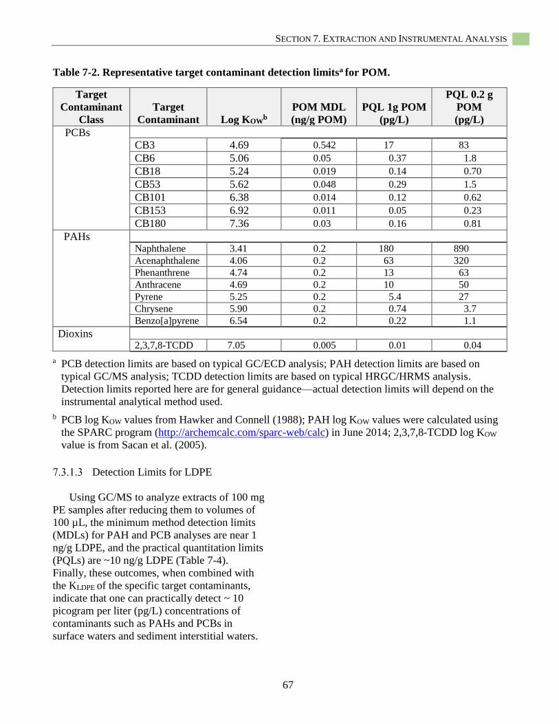
SECTION 7. EXTRACTION AND INSTRUMENTAL ANALYSIS
67
Table 7-2. Representative target contaminant detection limitsa for POM.
Target
Contaminant
Class
Target
Contaminant Log KOWb
POM MDL
(ng/g POM)
PQL 1g POM
(pg/L)
PQL 0.2 g
POM
(pg/L)
PCBs
CB3 4.69 0.542 17 83
CB6 5.06 0.05 0.37 1.8
CB18 5.24 0.019 0.14 0.70
CB53 5.62 0.048 0.29 1.5
CB101 6.38 0.014 0.12 0.62
CB153 6.92 0.011 0.05 0.23
CB180 7.36 0.03 0.16 0.81
PAHs
Naphthalene 3.41 0.2 180 890
Acenaphthalene 4.06 0.2 63 320
Phenanthrene 4.74 0.2 13 63
Anthracene 4.69 0.2 10 50
Pyrene 5.25 0.2 5.4 27
Chrysene 5.90 0.2 0.74 3.7
Benzo[a]pyrene 6.54 0.2 0.22 1.1
Dioxins 2,3,7,8-TCDD 7.05 0.005 0.01 0.04
a PCB detection limits are based on typical GC/ECD analysis; PAH detection limits are based on
typical GC/MS analysis; TCDD detection limits are based on typical HRGC/HRMS analysis.
Detection limits reported here are for general guidance—actual detection limits will depend on the
instrumental analytical method used.
b PCB log KOW values from Hawker and Connell (1988); PAH log KOW values were calculated using
the SPARC program (http://archemcalc.com/sparc-web/calc) in June 2014; 2,3,7,8-TCDD log KOW
value is from Sacan et al. (2005).
Detection Limits for LDPE
Using GC/MS to analyze extracts of 100 mg
PE samples after reducing them to volumes of
100 µL, the minimum method detection limits
(MDLs) for PAH and PCB analyses are near 1
ng/g LDPE, and the practical quantitation limits
(PQLs) are ~10 ng/g LDPE (Table 7-4).
Finally, these outcomes, when combined with
the KLDPE of the specific target contaminants,
indicate that one can practically detect ~ 10
picogram per liter (pg/L) concentrations of
contaminants such as PAHs and PCBs in
surface waters and sediment interstitial waters.
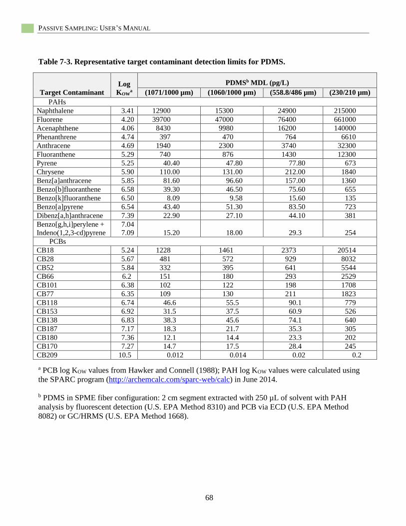
PASSIVE SAMPLING: USER’S MANUAL
68
Table 7-3. Representative target contaminant detection limits for PDMS.
Target Contaminant
Log
KOWa
PDMSb MDL (pg/L)
(1071/1000 µm) (1060/1000 µm) (558.8/486 µm) (230/210 µm)
PAHs
Naphthalene 3.41 12900 15300 24900 215000
Fluorene 4.20 39700 47000 76400 661000
Acenaphthene 4.06 8430 9980 16200 140000
Phenanthrene 4.74 397 470 764 6610
Anthracene 4.69 1940 2300 3740 32300
Fluoranthene 5.29 740 876 1430 12300
Pyrene 5.25 40.40 47.80 77.80 673
Chrysene 5.90 110.00 131.00 212.00 1840
Benz[a]anthracene 5.85 81.60 96.60 157.00 1360
Benzo[b]fluoranthene 6.58 39.30 46.50 75.60 655
Benzo[k]fluoranthene 6.50 8.09 9.58 15.60 135
Benzo[a]pyrene 6.54 43.40 51.30 83.50 723
Dibenz[a,h]anthracene 7.39 22.90 27.10 44.10 381
Benzo[g,h,i]perylene +
Indeno(1,2,3-cd)pyrene
7.04
7.09 15.20 18.00 29.3 254
PCBs
CB18 5.24 1228 1461 2373 20514
CB28 5.67 481 572 929 8032
CB52 5.84 332 395 641 5544
CB66 6.2 151 180 293 2529
CB101 6.38 102 122 198 1708
CB77 6.35 109 130 211 1823
CB118 6.74 46.6 55.5 90.1 779
CB153 6.92 31.5 37.5 60.9 526
CB138 6.83 38.3 45.6 74.1 640
CB187 7.17 18.3 21.7 35.3 305
CB180 7.36 12.1 14.4 23.3 202
CB170 7.27 14.7 17.5 28.4 245
CB209 10.5 0.012 0.014 0.02 0.2
a PCB log KOW values from Hawker and Connell (1988); PAH log KOW values were calculated using
the SPARC program (http://archemcalc.com/sparc-web/calc) in June 2014.
b PDMS in SPME fiber configuration: 2 cm segment extracted with 250 µL of solvent with PAH
analysis by fluorescent detection (U.S. EPA Method 8310) and PCB via ECD (U.S. EPA Method
8082) or GC/HRMS (U.S. EPA Method 1668).
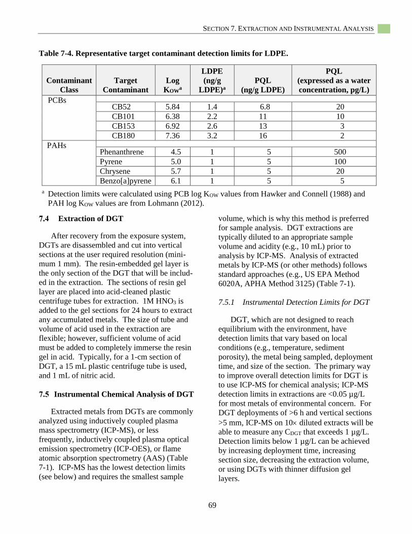
SECTION 7. EXTRACTION AND INSTRUMENTAL ANALYSIS
69
Table 7-4. Representative target contaminant detection limits for LDPE.
Contaminant
Class
Target
Contaminant
Log
KOWa
LDPE
(ng/g
LDPE)a
PQL
(ng/g LDPE)
PQL
(expressed as a water
concentration, pg/L)
PCBs CB52 5.84 1.4 6.8 20
CB101 6.38 2.2 11 10
CB153 6.92 2.6 13 3
CB180 7.36 3.2 16 2
PAHs Phenanthrene 4.5 1 5 500
Pyrene 5.0 1 5 100
Chrysene 5.7 1 5 20
Benzo[a]pyrene 6.1 1 5 5
a Detection limits were calculated using PCB log KOW values from Hawker and Connell (1988) and
PAH log KOW values are from Lohmann (2012).
Extraction of DGT
After recovery from the exposure system,
DGTs are disassembled and cut into vertical
sections at the user required resolution (mini-
mum 1 mm). The resin-embedded gel layer is
the only section of the DGT that will be includ-
ed in the extraction. The sections of resin gel
layer are placed into acid-cleaned plastic
centrifuge tubes for extraction. 1M HNO3 is
added to the gel sections for 24 hours to extract
any accumulated metals. The size of tube and
volume of acid used in the extraction are
flexible; however, sufficient volume of acid
must be added to completely immerse the resin
gel in acid. Typically, for a 1-cm section of
DGT, a 15 mL plastic centrifuge tube is used,
and 1 mL of nitric acid.
Instrumental Chemical Analysis of DGT
Extracted metals from DGTs are commonly
analyzed using inductively coupled plasma
mass spectrometry (ICP-MS), or less
frequently, inductively coupled plasma optical
emission spectrometry (ICP-OES), or flame
atomic absorption spectrometry (AAS) (Table
7-1). ICP-MS has the lowest detection limits
(see below) and requires the smallest sample
volume, which is why this method is preferred
for sample analysis. DGT extractions are
typically diluted to an appropriate sample
volume and acidity (e.g., 10 mL) prior to
analysis by ICP-MS. Analysis of extracted
metals by ICP-MS (or other methods) follows
standard approaches (e.g., US EPA Method
6020A, APHA Method 3125) (Table 7-1).
7.5.1 Instrumental Detection Limits for DGT
DGT, which are not designed to reach
equilibrium with the environment, have
detection limits that vary based on local
conditions (e.g., temperature, sediment
porosity), the metal being sampled, deployment
time, and size of the section. The primary way
to improve overall detection limits for DGT is
to use ICP-MS for chemical analysis; ICP-MS
detection limits in extractions are <0.05 µg/L
for most metals of environmental concern. For
DGT deployments of >6 h and vertical sections
>5 mm, ICP-MS on 10 diluted extracts will be
able to measure any CDGT that exceeds 1 µg/L.
Detection limits below 1 µg/L can be achieved
by increasing deployment time, increasing
section size, decreasing the extraction volume,
or using DGTs with thinner diffusion gel
layers.
PASSIVE SAMPLING: USER’S MANUAL
70
Section 8
Data Analysis: Calculation of Cfree and
CDGT
Introduction
In this section, for hydrophobic organic
contaminants, three methods are discussed for
using the passive sampler concentration data
for the target contaminants determined in
Section 7, with instrumental analysis, to
calculate the target contaminant’s Cfree. For the
hydrophobic organic contaminant passive
samplers (i.e., POM, PDMS, LDPE), there are
four basic approaches for handling the data
analysis (Figure 8-1). The first approach
assumes that the target contaminants achieved
equilibrium with the passive sampler and other
environmental phases during the deployment.
This assumption can be based on previous
experience with the passive sampler, the
deployment site, or the design of the passive
sampler investigation. In this approach,
relatively simple equations can be applied to
calculate Cfree using the passive sampler
concentration (CPS) data. These equations are
discussed below. The next two approaches
directly determine if the passive sampler and
target contaminants have achieved equilibrium.
In one approach, multiple thicknesses of POM,
PDMS and LDPE are deployed and the
concentrations of target contaminants on a
mass or volume of passive sampler basis are
compared. When the mass of target
contaminant is the same between different
thicknesses as a function of time, equilibrium
has been achieved. In the third approach,
multiple samplers are deployed and collected at
varying times to develop a time series. Like
the multiple thicknesses approach, when the
concentration of target contaminant in the
passive samplers no longer changes
significantly with time, equilibrium has been
reached. These two approaches benefit by
providing definitive evidence that equilibrium
has occurred between the target contaminants
and the passive samplers. However, these
approaches both require addition deployments
of passive samplers and chemical analyses
which will increases overall costs. For ex situ
deployments, these methods may be
worthwhile (see the discussion of different
thicknesses of PDMS in Section 3.1) but in
in situ deployments, the additional field effort
and analytical chemistry may be prohibitively
expensive.
In another approach, and the one
recommended in this document, equilibrium is
not assumed to have occurred among the target
contaminants, the passive sampler, and other
environmental phases. In this case, losses of the
performance reference compounds (PRCs)
discussed in Section 6 are used to adjust the
passive sampler concentration data from non-
equilibrium concentrations to equilibrium Cfree
values. The use of PRCs to calculate Cfree,
while scientifically sound, is still an evolving
practice with the potential to become
complicated because of the multiple variables
included in the calculations. In order to build in
a degree of consistency into the application of
PRCs, the use of three standardized PRC
correction calculators (PCCs) accessed via
graphic user interfaces (GUIs) for (1) PDMS
passive sampling in a SPME fiber configuration,
(2) LDPE passive sampling in sediments, and
(3) LDPE passive sampling in the water column

SECTION 8. DATA ANALYSIS
71
is encouraged to ensure that all of the PRC
calculations are performed uniformly.
Figure 8-2 provides a flow chart for selecting
the appropriate GUI to use for calculating Cfree
based on the type of polymer deployed and the
kind of deployment (i.e., water column versus
sediments) for LDPE and POM. The LDPE
GUI can be applied with POM recognizing that
the input values have to be changed to reflect
the POM-specific variables like POM and water
diffusion coefficients and POM partition
coefficients.
The PDMS GUI and an Excel spreadsheet
version of the PDMS GUI can be downloaded
from this web address:
http://www.depts.ttu.edu/ceweb/groups/reiblesg
roup/downloads.html
The sediment deployment LDPE GUI can
be downloaded from the following web
addresses:
https://www.serdp-estcp.org/Tools-and-
Training/Tools/PRC-Correction-Calculator
and
https://www.epa.gov/superfund/superfund-
contaminated-sediments-guidance-documents-
fact-sheets-and-policies
Additional guidance on the sediment
deployment LDPE GUI is located here:
https://www.serdp-estcp.org/Program-
Areas/Environmental-
Restoration/Contaminated-Sediments/ER-
200915
Finally, the water column LDPE GUI and
additional guidance can be downloaded from
the following address:
https://www.epa.gov/superfund/superfund-
contaminated-sediments-guidance-documents-
fact-sheets-and-policies
Figure 8-3 illustrates the data entry points and
lay-out of the PDMS GUI while Figure 8-4
provides an example output from the PDMS
GUI. Figures 8-5 and 8-6 report information
for the sediment LDPE GUI and Figures 8-7,
8-8 and 8-9 show similar information for the
water column LDPE GUI. Note that some of
the partition coefficients used by the sediment
LDPE GUI differ from those provided in
Appendix A of this document but that the PCC
GUI allows the user to select which coefficients
to use.
The PCCs discussed here are highlighted
because GUIs have been developed to simplify
their use. Booij and Smedes (2010) describe an
alternative PCC that document users are
encouraged to investigate. This PCC is
spreadsheet-based and can be accessed by
contacting the authors of Booij and Smedes
(2010).
The approach for performing the DGT data
analysis results in the calculation of CDGT
(Figure 8-1). This data analysis is unique for
metals and is discussed below.
POM, PDMS, and LDPE Data
Analysis
Figures 8-1 and 8-2 provide flowcharts for
determining how to proceed with the data
analysis of passive sampler concentration data.
The starting point for the data analysis is to
have the concentration of target contaminants
in the various passive sampler media (e.g.,
POM, PDMS, LDPE, DGT gel). For example,
x µg CB52 /g POM.
PASSIVE SAMPLING: USER’S MANUAL
72
Equilibrium Conditions
Under demonstrated or assumed
equilibrium conditions, Equation 8-1 can be
applied to calculate Cfree for hydrophobic
organic target contaminants using measured
passive sampler concentrations CPS (more
specifically, CPOM, CPDMS, CLDPE) and the
appropriate partition coefficient (KPS) (more
specifically, KPOM, KPDMS, KLDPE):
PS
PS
freeK
CC [8-1]
Non-Equilibrium Conditions using
PRCs
Because passive sampler deployments are
commonly too short for target contaminants to
achieve equilibration with their surroundings,
particularly for larger, high KOW target
contaminants, PRCs were developed as a tool
to estimate the degree of disequilibria between
the target contaminants associated with the
passive sampler and the rest of the
environmental phases. The GUI discussed
above calculate a simple variable, the fractional
equilibria (feq) (expressed as a decimal), which
can be used to adjust the measured non-
equilibrium passive sampler concentration
(CPS), from Section 7, to equilibrium
conditions:
PS
eq
PS
freeK
f
C
C
[8-2]
However, before feq can be calculated with a
GUI, it is necessary to estimate the actual feq
based on the measured PRC concentrations in
the deployed passive samplers and the non-
deployed passive samplers:
x
PRC
x
PRC
x
PRCxm
eq
i
fi
c
ccPRCf
[8-3]
where, fmeq PRCx is the measured fractional
equilibrium for PRC x (in contrast to the
calculated feq generated by the GUIs for the
target contaminants), CxPRCf
is the passive
sampler concentration of PRC x (µg/g polymer)
following deployment, and CxPRCi is the passive
sampler concentration of PRC x that was
loaded with PRCs but not deployed (i.e., stored
in the dark at -4˚C until chemical analysis with
the deployed passive samplers). The fmeq PRC
x values, in decimal format, will be loaded into
the PCCs via the GUIs.
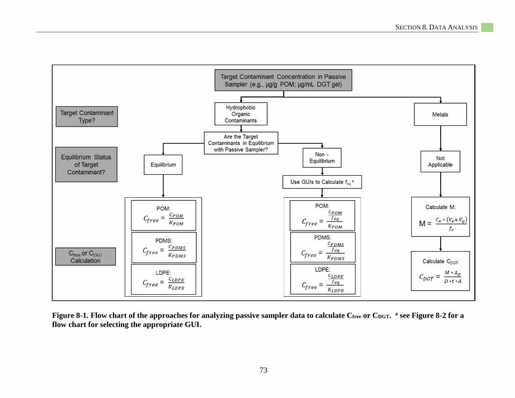
SECTION 8. DATA ANALYSIS
73
Figure 8-1. Flow chart of the approaches for analyzing passive sampler data to calculate Cfree or CDGT. a see Figure 8-2 for a
flow chart for selecting the appropriate GUI.

PASSIVE SAMPLING: USER’S MANUAL
74
Figure 8-2. Flow chart for selecting the appropriate PRC Correction Calculator GUI for analyzing non-equilibrium
hydrophobic organic contaminant passive sampling data to calculate Cfree. a to use the GUIs cited in this figure with POM,
the user will need to change the GUI’s input values for the POM polymer.
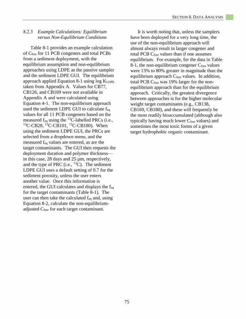
SECTION 8. DATA ANALYSIS
75
Example Calculations: Equilibrium
versus Non-Equilibrium Conditions
Table 8-1 provides an example calculation
of Cfree for 11 PCB congeners and total PCBs
from a sediment deployment, with the
equilibrium assumption and non-equilibrium
approaches using LDPE as the passive sampler
and the sediment LDPE GUI. The equilibrium
approach applied Equation 8-1 using log KLDPE
taken from Appendix A. Values for CB77,
CB126, and CB169 were not available in
Appendix A and were calculated using
Equation 4-1. The non-equilibrium approach
used the sediment LDPE GUI to calculate feq
values for all 11 PCB congeners based on the
measured feq using the 13C-labelled PRCs (i.e., 13C-CB28, 13C-CB101, 13C-CB180). When
using the sediment LDPE GUI, the PRCs are
selected from a dropdown menu, and the
measured feq values are entered, as are the
target contaminants. The GUI then requests the
deployment duration and polymer thickness—
in this case, 28 days and 25 µm, respectively,
and the type of PRC (i.e., 13C). The sediment
LDPE GUI uses a default setting of 0.7 for the
sediment porosity, unless the user enters
another value. Once this information is
entered, the GUI calculates and displays the feq
for the target contaminants (Table 8-1). The
user can then take the calculated feq and, using
Equation 8-2, calculate the non-equilibrium-
adjusted Cfree for each target contaminant.
It is worth noting that, unless the samplers
have been deployed for a very long time, the
use of the non-equilibrium approach will
almost always result in larger congener and
total PCB Cfree values than if one assumes
equilibrium. For example, for the data in Table
8-1, the non-equilibrium congener Cfree values
were 13% to 80% greater in magnitude than the
equilibrium approach Cfree values. In addition,
total PCB Cfree was 19% larger for the non-
equilibrium approach than for the equilibrium
approach. Critically, the greatest divergence
between approaches is for the higher molecular
weight target contaminants (e.g., CB138,
CB169, CB180), and these will frequently be
the most readily bioaccumulated (although also
typically having much lower Cfree values) and
sometimes the most toxic forms of a given
target hydrophobic organic contaminant.

PASSIVE SAMPLING: USER’S MANUAL
76
Figure 8-3. Primary data entry points and basic layout of the graphical user interface (GUI) for the PDMS PRC Correction
Calculator

SECTION 8. DATA ANALYSIS
77
Figure 8-4. Example output from the GUI for the PDMS PRC Correction Calculator
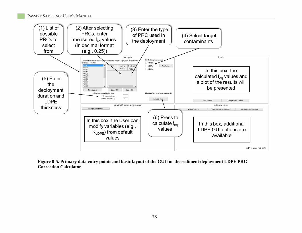
PASSIVE SAMPLING: USER’S MANUAL
78
Figure 8-5. Primary data entry points and basic layout of the GUI for the sediment deployment LDPE PRC
Correction Calculator

SECTION 8. DATA ANALYSIS
79
Figure 8-6. Example output from the GUI for the sediment deployment LDPE PRC Correction Calculator

PASSIVE SAMPLING: USER’S MANUAL
80
Figure 8-7. Primary data entry points and basic layout of the GUI for the water column
deployment LDPE PRC Correction Calculator
Figure 8-8. Example of data entry window (‘UserForm1’)for the water column LDPE PRC
Correction Calculator

SECTION 8. DATA ANALYSIS
81
Figure 8-9. Example output from the GUI for the water column deployment LDPE PRC
Correction Calculator
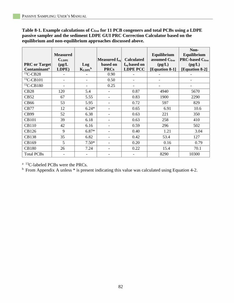
PASSIVE SAMPLING: USER’S MANUAL
82
Table 8-1. Example calculations of Cfree for 11 PCB congeners and total PCBs using a LDPE
passive sampler and the sediment LDPE GUI PRC Correction Calculator based on the
equilibrium and non-equilibrium approaches discussed above.
PRC or Target
Contaminanta
Measured
CLDPE
(µg/L
LDPE)
Log
KLDPEb
Measured feq
based on
PRCs
Calculated
feq based on
LDPE PCC
Equilibrium
assumed Cfree
(pg/L)
[Equation 8-1]
Non-
Equilibrium
PRC-based Cfree
(pg/L)
[Equation 8-2] 13C-CB28 - - 0.90 - - - 13C-CB101 - - 0.50 - - - 13C-CB180 - - 0.25 - - -
CB28 120 5.4 - 0.87 4940 5670
CB52 67 5.55 - 0.83 1900 2290
CB66 53 5.95 - 0.72 597 829
CB77 12 6.24* - 0.65 6.91 10.6
CB99 52 6.38 - 0.63 221 350
CB101 39 6.18 - 0.63 258 410
CB110 42 6.16 - 0.59 296 502
CB126 9 6.87* - 0.40 1.21 3.04
CB138 35 6.82 - 0.42 53.4 127
CB169 5 7.50* - 0.20 0.16 0.79
CB180 26 7.24 - 0.22 15.4 70.1
Total PCBs - - - - 8290 10300
a 13C-labeled PCBs were the PRCs. b From Appendix A unless * is present indicating this value was calculated using Equation 4-2.

SECTION 8. DATA ANALYSIS
83
DGT Data Analyses
Following the extraction and analyses for
metals discussed in Section 7, the metal
concentrations in the DGT gel extract are used
to calculate a mass associated with the resin gel
(M in µg) (Figure 5-1):
e
gee
f
VVCM
*[8-4]
where, Ce is the metal concentration in the acid
extract (µg/mL), Ve is the volume of the acid
extract plus any volume used for dilution (mL),
Vg is the volume of the gel (mL), and fe is the
elution factor. For standard DGT disks (i.e.,
resin gel thickness of 0.4 mm), Vg is 0.196 mL.
For the DGT probes, Vg can be calculated using
the formula for the volume of a rectangular
prism (i.e., Vg = length*width*height) (h =
0.04 cm, w = 1.8 cm); for example, a 1-cm
vertical section length of gel has a volume of
0.072 mL. The elution factor may be necessary
if 1M HNO3 does not completely extract all of
the metal from the resin gel. For Zn, Cd, Cu,
Ni, Pb, and Mn, a fe value of 0.8 can be used,
and for Fe, a fe value of 0.7 can be used.
Alternatively, matrix spikes can be performed
to determine elution recoveries. With the mass
on the resin gel calculated, the concentration of
metal at the surface of the DGT device (CDGT in
µg/mL) can be calculated as:
AtD
MC
d
g
DGT**
* [8-5]
where, Δg is thickness of the diffusive gel and
membrane filter (cm), D is the diffusion
coefficient in the gel (cm2/s), td is the time of
deployment (s), and A is the surface area of the
DGT exposed to the sediment (cm2). For both
disk and probe assemblies, standard DGTs have
Δg of 0.93 mm. Metal diffusion in the DGT
gel increases with increasing temperature
following a polynomial function. D in the
DGT diffusive gel has been calculated for
11 metals for temperatures from 1 to 35°C
(Appendix D). For DGT disks, A is 3.14 cm2,
and for DGT probes, A is determined by the
size of the sectioned resin gel (e.g., 1.8 cm2 for
a 1-cm vertical section).
Example DGT Calculations
As an example calculation, if a 1-cm
section of a standard DGT probe (Vg = 0.072
mL) was dissolved in 1 mL of nitric acid
(HNO3), Ve = 1.0 mL, and a Ni concentration in
the extract of 869 µg/L was analytically
measured, using Equation 8-4, the nickel mass
bound to the gel (M) would be calculated as
1.16 µg. Next, using Equation 8-5, if the DGT
had been deployed for 23 h at 18.3°C, a CDGT
of 152 µg/L would be calculated.
Case Studies
To illustrate the application of passive
sampling, the following case studies are
included in Appendix F of the document:
Case Study 1: Lower Grasse River, New York,
USA
Case Study 2: Pacific Sound Resources
Superfund Site (Marine Sediment Unit), Seattle,
Washington, USA
Case Study 3: Wyckoff/Eagle Harbor Superfund
Site (East Harbor Operable Unit), Bainbridge
Island, Washington, USA
Case Study 4: United Heckathorn Superfund Site
(Lauritzen Channel, Inner Richmond Harbor),
California, USA
Case Study 5: Site Assessment of Sediment
Toxicity, San Diego Bay, California, USA
Case Study 6: Ex situ Passive Sampling
Measurement of Site-Specific Partitioning of
PAHs and PCBs in Sediments
These case studies provide a comprehensive
demonstration of the preparation, deployment,
recovery, and data analysis of various types of
passive samplers discussed in this document.
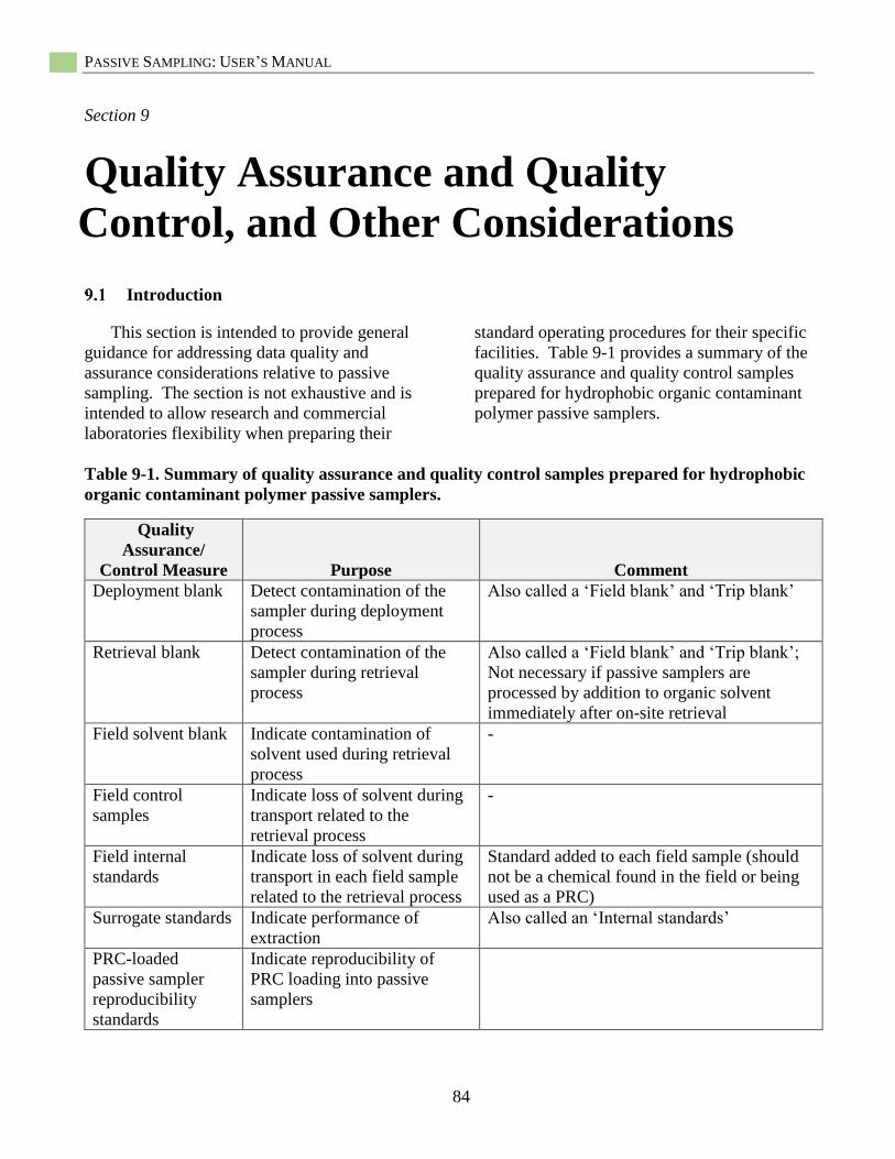
PASSIVE SAMPLING: USER’S MANUAL
84
Section 9
Quality Assurance and Quality
Control, and Other Considerations
Introduction
This section is intended to provide general
guidance for addressing data quality and
assurance considerations relative to passive
sampling. The section is not exhaustive and is
intended to allow research and commercial
laboratories flexibility when preparing their
standard operating procedures for their specific
facilities. Table 9-1 provides a summary of the
quality assurance and quality control samples
prepared for hydrophobic organic contaminant
polymer passive samplers.
Table 9-1. Summary of quality assurance and quality control samples prepared for hydrophobic
organic contaminant polymer passive samplers.
Quality
Assurance/
Control Measure Purpose Comment
Deployment blank Detect contamination of the
sampler during deployment
process
Also called a ‘Field blank’ and ‘Trip blank’
Retrieval blank Detect contamination of the
sampler during retrieval
process
Also called a ‘Field blank’ and ‘Trip blank’;
Not necessary if passive samplers are
processed by addition to organic solvent
immediately after on-site retrieval
Field solvent blank Indicate contamination of
solvent used during retrieval
process
-
Field control
samples
Indicate loss of solvent during
transport related to the
retrieval process
-
Field internal
standards
Indicate loss of solvent during
transport in each field sample
related to the retrieval process
Standard added to each field sample (should
not be a chemical found in the field or being
used as a PRC)
Surrogate standards Indicate performance of
extraction
Also called an ‘Internal standards’
PRC-loaded
passive sampler
reproducibility
standards
Indicate reproducibility of
PRC loading into passive
samplers
SECTION 9. QUALITY ASSURANCE AND QUALITY CONTROL
85
Hydrophobic Organic Contaminant
Polymer-Specific Quality Assurance
and Quality Control
Polymer-Specific Deployment Blanks
(i.e., trip blanks, field blanks)
The polymers used for passive sampling
have high partition coefficients for hydrophobic
organics, so there is a significant chance of
contaminating the polymers via exposure to the
laboratory or field environment. Passive
samplers used for measurement should be
protected from the laboratory and field
environment through adequate containment and
storage in clean glass jars (i.e., solvent washed
and muffled). Such contamination problems
are especially important when measurements
are being performed at low concentrations and
background reference sites, and the types of
target contaminants being measured are
ubiquitous in the environment, such as low
molecular weight PAHs. Thus, every passive
sampling investigation should include an
adequate set of laboratory and field blanks.
The laboratory performing the passive
sampling measurements should demonstrate the
absence of contamination of field and
laboratory blanks at the practical quantitation
limits. In addition, the laboratory should
demonstrate that no significant loss of loaded
PRCs occurred before sampler deployment in
the field. Maintaining loaded samplers at 4˚C
or less prior to deployment will limit PRC
losses.
A deployment blank should be employed
during the deployment. The deployment blank
is a sampler that is shipped together with other
samplers (i.e., deployed) to the field but is
shipped back without being deployed. A
retrieval blank is a sampler that is shipped
together with the other samplers on retrieval,
but is not needed if the samplers are processed
immediately on retrieval. Both the recovery
and retrieval blanks will include PRCs if the
regular passive samplers being deployed and
retrieved include PRCs. The field blanks
are used to assess possible presence of
environmental contamination during
deployment activities. Field blanks should
have no significant peaks where PRCs,
surrogate standards, injection standards,
and target analytes occur (<0.1 ng/g passive
sampler).
Field Solvent Blanks
For studies in which solvent will be added
to vials containing the recovered samplers, a
field solvent blank should be included. Field
solvent blanks will be analyzed at the time of
filling the vials for shipment (i.e., one at the
start of filling the vials and one at the end
where the same solvent source, has been used).
If these contain target contaminants at
significant levels, new vials will be filled from
a separate source, and the process will be
repeated. In addition, solvent blanks should be
shipped with the samples at a frequency of 1
per 20 samples.
Field Control Samples
Field control samples are used to track the
solvent volume change of contamination during
transport if on-site processing of samplers is
performed. The field control samples can be
calibration standards or other solutions with
known concentrations (note: if using calibration
standards, these same standards should not be
used for the analytical instrumental
calibration). The field control samples are
treated identically as other samples. At least
five field control samples are needed for each
deployment. They can be five different
concentrations or five replicates of the same
concentration if estimations of field
concentrations are available. The average of
the concentration change for all compounds in
all field control samples should be within 15%
to avoid the need to make solvent volume
adjustments.
PASSIVE SAMPLING: USER’S MANUAL
86
Field Internal Standards
Although field control samples indicate
solvent stability during transport, internal
standards are recommended for field samples to
indicate any changes in solvent loss in
individual samples. Deuterated PAHs and 13C12-labelled PCB congeners are good choices
for internal standards. If an internal standard
is used it should be included in the extraction
vials. The chosen compound should not be
present in the field in significant quantities and
should not be used as a PRC. The average of
the concentration changes for all internal
standards added in each sample should be
within 15% of a laboratory prepared field
internal standard (assume no losses in this
standard) to avoid the need to make solvent
volume adjustments to account for losses
while in the field.
Recoveries of Surrogate Standards
(also known as Internal Standards)
Surrogate standards should be recovered
from passive sampling samples at 100%, plus
or minus analytical precision, >70% to <120%.
An exception may be relatively volatile
compounds (e.g., mono-, dichlorobiphenyls)
that can be lost in significant amounts when
extracts are evaporated (e.g., recovery down to
60%). Typical surrogates used for PCB
analysis in the GC/ECD analytical method are:
PCB-14, PCB-65, and PCB-166.
PRC-Loaded Passive Sampler
Reproducibility
Individual batches of passive samplers
loaded with PRCs should exhibit reproducible
PRC concentrations (e.g., coefficient of
variation <20%) in the passive sampler before
deployment.
QC Samples for Chemical Analysis
The QC samples for chemical analysis of
PAHs and PCBs, including initial calibration,
second-source standard check, and continued
calibration verification checks should meet the
acceptance criterion set in the analytical
methods of each laboratory. These QC
standards are not unique to passive sampling.
A complete set of example guidelines for
quality assurance and quality control (QA/QC)
based on the U.S. Department of Defense
Quality Management System (QMS) can be
found in Appendix E. These guidelines are not
intended as required but are provided as
examples.
Specific Quality Assurance for POM
When correct procedures are followed
in the use of POM in passive sampling
applications, the analytical results have high
accuracy and reproducibility. Key to the
success of any passive sampling approach is the
accurate determination of polymer partitioning
constants for the target contaminants of
interest. A recent report by Arp et al. (2015)
reviewed reported results from six studies for
PCBs and three studies for PAHs and found
that the majority of the differences could be
attributed to different thicknesses of POM used
(lack of equilibrium) and different extraction
procedures applied. They report that when the
correct thickness of POM (≤76 m) and a
hexane-acetone mixture are used for the
extraction of this polymer, the reported KPOM
values for PCBs and PAHs are highly
reproducible (e.g., within 0.2 log units).
Thus, for POM, it is critical to ensure that the
thickness of POM used is 76 m or less.
Also, it is very important to use the same POM
as used in the KPOM determination. This point
is also true for PDMS and LDPE. The most
widely used KPOM values are for the 76 m
POM from CS Hyde Company (Table 1-1)
which is made with an ethylene oxide
copolymer.
SECTION 9. QUALITY ASSURANCE AND QUALITY CONTROL
87
Most of the published studies have reported
use of POM in the determination of equilibrium
aqueous concentrations in sediments based on
ex situ laboratory experiments. At the time of
this publication, there have been few studies of
in situ application of POM with performance
reference compound (PRC) corrections.
Specific Quality Assurance for PDMS
Use of PDMS can result in high analytical
accuracy and reproducibility (Thomas et al.
2014). A calibration study of the PDMS fiber
in prepared water with PAHs found that the
linearity of the resulting calibration for mid-
range HOCs was very high with r2 = 0.99
(Reible 2010). Coefficients of variation from
the resulting linear curve were less than 20%
for all PAH compounds except naphthalene.
Naphthalene does not concentrate significantly
on the PDMS fiber, and losses to air are rapid,
making it difficult to measure naphthalene via
PDMS without increasing the PDMS layer
volume. Coefficients of variation by
conventional extraction methods have also been
seen to be 10% to 20%, suggesting that the
levels of accuracy of the PDMS methods were
essentially identical to that expected by
conventional methods. Like POM, to ensure
acceptable data quality assurance, it is very
important, whenever possible, to use the same
batch and thickness of PDMS for developing
KPDMS values as for performing actual
deployments.
Specific Quality Assurance for LDPE
The first concern when using all of the
polymers, including LDPE, is to quantify
organic contaminants, especially in interstitial
waters, as accurately as possible. Several
investigations have been pursued to test this
measurement for LDPE. First, Fernandez et al.
(2009a, b) used ex situ testing with sediments
from three sites (two in Boston Harbor and one
in San Francisco Bay) to demonstrate that
PRC-corrected measures of PAHs in interstitial
water were very close to direct measures of the
PAHs in isolated interstitial waters, after
making corrections for the presence of colloid-
bound PAHs in the water samples. Further,
Gschwend et al. (2011) used ex situ testing of
PCB-contaminated sediments from Hunters
Point in San Francisco Bay to test the accuracy
of the LDPE approach. As an independent
reference, air bridge sampling was used to
avoid problems with other partitioning phases
(e.g., colloids); a set of six replicates revealed
that congener 101 (2, 2', 4, 5, 5'-pentachloro-
biphenyl) was present at a little less than 1 ng/L
in the interstitial water. Isolation of the
interstitial water and its analysis suggested a
concentration near 5 ng/L, until corrections for
colloid-associations were used and lowered the
estimated interstitial water concentration to
about 2 ng/L. Using the commonly applied
equilibrium partitioning modelling suggested a
interstitial water concentration of 32 ng/L; this
result was clearly divergent from the air
bridges. Correcting this approach by using a
sorption coefficient that included adsorption to
black carbon measured in this sediment (see
Lohmann et al. 2005) lowered the estimated
interstitial water concentration to less than
0.5 ng/L. Finally, analyses of multiple LDPE
samplers left in the sediment for a week, and
another set for a month, resulted in PRC-
corrected interstitial water concentrations of
about 1 and about 0.5 ng/L, respectively.
Clearly, the use of the LDPE samplers was
much more accurate than equilibrium
partitioning modelling, and the LDPE results
matched the air bridges to within a factor of 2.
Like POM and PDMS, to ensure acceptable
data quality assurance, it is very important,
whenever possible, to use the same batch and
thickness of LDPE for developing KLDPE values
as for performing actual deployments.

PASSIVE SAMPLING: USER’S MANUAL
88
Passive Sampling Example Sampling
and Analysis Project Plan (SAP) and
Quality Assurance Project Plan
(QAPP)
Appendix G contains two documents that are
intended to assist the reader in the preparation
of future QAPPs involving passive sampling.
The first document is the Sampling and
Analysis Plan for River Mile 11 East (RM11E)
Study Area. The RM11E study was conducted
to supplement the Portland Harbor Superfund
Site (Portland Harbor) Draft Investigation.
The goal of the investigation was to collect
interstitial water data for input into a sediment
cap isolation model and to inform cap design.
Appendix G also includes a copy of the
QAPP prepared for the 2011 deployment of
LDPE samplers at the Palos Verdes Shelf
Superfund site off the coast of Los Angeles
(California, USA). Goals of the deployment
were to investigate the release of target
contaminants from the contaminated sediment
into the water column.
DGT-Specific Quality Assurance
and Quality Control
DGT Quality Control
There is a risk of contamination during
preparation, transport, storage, and handling
of the DGTs, so a field blank should be used
to best account for this possible contamination
(Knutsson et al. 2014). DGT field blanks
should be extracted and analyzed using the
same procedures completed for those deployed
(Villanueva et al. 2013). For all deployments,
at least (triplicate blanks are preferred) one
extra DGT should be deoxygenated, marked,
and processed in the same manner as all other
DGTs with the exception of being exposed to
sediment. This “control” DGT is used to verify
that the solution used to deoxygenate the
probes and any associated handling does not
introduce any metal contamination to the
DGTs. Blank values should then be subtracted
from the values obtained from the field
deployed DGTs (Villanueva et al. 2013).
Additionally, all equipment (e.g., storage
vessel, forceps, centrifuge tubes, gel sectioning
plate) should be acid-cleaned with >1M acid to
ensure that no metals are introduced during use
and processing.
DGT Quality Assurance
A potential concern with DGTs is
uncertainty in the measurements including
error in the thickness of the diffusive gel and
the cross sectional diffusive area (Warnken
et al. 2006). A recent paper suggested the
measured values for diffusive gel thickness
were 1.1%-2.2% smaller than their nominal
value and sampling area was generally
underestimated by 1.4 µm (Kruzeder et al.
2015). When grouping the total uncertainties
from DGT sampling under well-controlled
experimental conditions, including sample
preparation and analytical work, uncertainties
of 0.3-3.3% for low target contaminant
concentration case studies and 3-6% for higher
target contaminant concentra-tions were
identified (Kruzeder et al. 2015).
Understanding the diffusive boundary layer
(DBL) that forms on the exposed side of the
device can be important to the performance of
effective DGT techniques (Turner et al. 2014).
The DBL has been identified as a possible
factor in ensuring accurate time-weighted
average concentrations. For well-controlled
laboratory experiments and/or in situ field
deployments where absolute accuracy is not a
concern, the DBL can generally be negated
(Warnken et al. 2006). However, when
accuracy and precision are important, the DBL
should be estimated as effectively as possible
and included in expanded DGT equations (see
Turner et al. 2014, Warnken et al. 2006,
Kreuzeder et al. 2015). Accounting for the
DBL is particularly important for longer term
deployments and in systems with fluctuating
SECTION 9. QUALITY ASSURANCE AND QUALITY CONTROL
89
flows, high suspended particular matter, and/or
biofouling, where the exclusion of the DBL in
calculations can lead to significantly
underestimated concentrations (Turner et al.
2014). Although actually measuring the DBL
for DGTs is not readily possible, the thickness
can be estimated in some circumstances. For
example, if DGTs are deployed in systems with
a high flowrate and elevated turbulence, the
DBL will be close to zero. Also, if the DGT is
oriented so that the surface of the filter
membrane is perpendicular to the flow, the
DBL will be negligible. For non-flowing
systems, placing the DGT near the water
surface where wind and wave action will mix
the water, the DBL will approach smaller, less
important values. Continuing to identify these
key uncertainties and optimizing these areas
should help reduce the uncertainties of DGT
techniques (Knutsson et al. 2014).
PASSIVE SAMPLING: USER’S MANUAL
90
Section 10
References Accardi-Dey A, PM Gschwend. 2002.
Assessing the combined roles of natural
organic matter and black carbon as sorbents in
sediments. Environ Sci Technol 36: 21-29.
Adams RG, Lohmann R, Fernandez LA,
MacFarlane JK, Gschwend PM. 2007.
Polyethylene devices: Passive samplers for
measuring dissolved hydrophobic organic
compounds in aquatic environments. Environ
Sci Technol 41(4):1317–1323.
Adams WJ, Kimerle RA, Mosher RG. 1985.
Aquatic safety assessment of chemicals sorbed
to sediments. In: Cardwell RD, Purdy R,
Bahner RC, editors. Aquatic toxicology and
hazard assessment: Seventh symposium.
Philadelphia (PA): ASTM. ASTM STP 854.
p 429–453.
Ahn S, Werner D, Karapanagioti HK,
McGlothlin DR, Zare RN, Luthy RG. 2005.
Phenanthrene and pyrene sorption and
intraparticle diffusion in polyoxymethylene,
coke, and activated carbon. Environ Sci
Technol 39:6516–6526.
Allen HE, Fu G, Boothman W, DiToro DM,
Mahony JD. 1991. Determination of acid
volatile sulfide and selected simultaneously
extractable metals in sediment. EPA/821/12-
91/100. U.S. Environmental Protection
Agency, Washington, DC.
Ankley G, Di Toro D, Hansen D, Berry W.
1996. Assessing the ecological risk of metals in
sediments. Environ Toxicol Chem
15:2053–2055.
Apell JN, PM Gschwend. 2014. Validating the
use of performance reference compounds in
passive samplers to assess porewater
concentrations in sediment beds. Environ Sci
Technol 48:10301-10307.
Apell JN, Tcaciuc AP and Gschwend, P.M.
2015. Understanding the rates of nonpolar
organic chemical accumulation into passive
samplers deployed in the environment:
Guidance for passive sampler deployments.
Integr Environ Assess Manage 12:486-492.
Arp HP, Breedveld GD, Cornelissen G. 2009.
Estimating the in situ sediment-porewater
distribution of PAHs and chlorinated aromatic
hydrocarbons in anthropogenic impacted
sediments. Environ Sci Technol 43(15):
5576–5585.
Arp HP, Hale SE, Krusa ME, Cornelissen G,
Grabanski CB, Miller DJ, Hawthorne SB.
2015. Review of polyoxymethylene passive
sampling methods for quantifying freely
dissolved porewater concentrations of
hydrophobic organic contaminants. Environ
Toxicol Chem 34: 710–720.
Arthur CL, Pawliszyn J. 1990. Solid phase
microextraction with thermal desorption using
fused silica optical fibers. Anal Chem
62(19):2145–2148.
Babut MP, Ahlf W, Batley GE, Camusso M,
Deckere ED, Besten PJD. 2005. International
overview of sediment quality guidelines and
their uses. In: Wenning RJ, Batley GE,
Ingersoll CG, Moore DW. (Eds.) Use of
Sediment Quality Guidelines and Related Tools
for the Assessment of Contaminated Sediments.
Society of Environmental Toxicology and
Chemistry Press, Pensacola, FL. pp. 345–381.
10. REFERENCES
91
Baker RA. 1980a. Contaminants and Sediments
Vol 1––Fate and Transport, Case Studies,
Modeling, Toxicity. Ann Arbor Science, Ann
Arbor, MI.
Baker RA. 1980b. Contaminants and Sediments
Vol 2––Analysis, Chemistry, Biology. Ann
Arbor Science, Ann Arbor, MI.
Bao LJ, You J, Zeng EY. 2011. Sorption of
PBDE in low-density polyethylene film:
implications for bioavailability of BDE-209.
Environ Toxicol Chem 30(8):1731–1738.
Barthe M, Pelletier E, Breedveld GD,
Cornelissen G. 2008. Passive samplers versus
surfactant extraction for the evaluation of PAH
availability in sediments with variable levels of
contamination. Chemosphere 71(8):1486–1493.
Baudo R, Giesy J, Muntau H. 1990. Sediments:
Chemistry and Toxicity of In-Place Pollutants.
Lewis, Boca Raton, FL.
Bayen SP, ter Laak TL, Buffle J, Hermens
JLM. 2009. Dynamic exposure of organisms
and passive samplers to hydrophobic
chemicals. Environ Sci Technol
43(7):2206–2215.
Beckingham B, Ghosh U. 2011. Field-scale
reduction of CB bioavailability with activated
carbon amendment to river sediments. Environ
Sci Technol 45(24):10567–10574.
Beckingham B, Ghosh U. 2013.
Polyoxymethylene passive samplers to monitor
changes in bioavailabilty and flux of PCBs
after activated carbon amendment to sediment
in the field. Chemosphere 91:1401–1407.
Beckingham B, Buys D, Vandewalker H,
Ghosh U. 2013. Observations of limited
secondary effects to benthic invertebrates and
macrophytes with activated carbon amendment
in river sediments. Environ Toxicol Chem
32(7):1504–1515.
Belzile N, De Vitre R, Tessier A. 1989. In situ
collection of diagenetic iron and manganese
oxyhydroxides from natural sediments. Nature
340:376–377.
Booij K, Sleiderink HM, Smedes F. 1998
Calibrating the uptake kinetics of
semipermeable membrane devices using
exposure standards. Environ Toxicol Chem
17(7):1236–1245.
Booij K, Smedes F, van Weerlee EM. 2002.
Spiking of performance reference compounds
in low density polyethylene and silicone
passive water samplers. Chemosphere
46(8):1157–1161.
Booij K, Smedes F. 2010. An improved method
for estimating in situ sampling rates of
nonpolar passive samplers. Environ Sci
Technol 44:6789–6794.
Brumbaugh WG, May T, Besser JM, Allert A,
Schmitt C. 2007. Assessment of elemental
concentrations in streams of the New Lead Belt
in southeastern Missouri 2002–05. Scientific
investigations report 2007–5057. U.S.
Geological Survey. 57 pp.
Burgess RM, Scott KJ. 1992. The Significance
of in-place contaminated marine sediments on
the water column: processes and effects. In;
Burton GA (ed.) Sediment Toxicity
Assessments. Lewis Publishers, Inc, Boca
Raton, FL, pp. 129–165.
Burgess RM, Berry DR, Mount DM, Di Toro
WJ. 2013. Critical review: Mechanistic
sediment quality guidelines based on
contaminant bioavailability: Equilibrium
partitioning sediment benchmarks (ESBs).
Environ Toxicol Chem 32:102–114.
Burton GA. 1992. Sediment Toxicity Assess-
ment. Lewis Publishers, Inc, Boca Raton, FL.

PASSIVE SAMPLING: USER’S MANUAL
92
Burton GA. 2010. Metal bioavailability and
toxicity in sediments. Crit Rev Env Sci Tec
40:852–907.
Burton GA, Nguyen LTH, Janssen C, Baudo R,
McWilliam RA, Bossuyt B, Beltrami M, Green
A. 2005. Field validation of sediment zinc
toxicity. Environ Toxicol Chem 24:541–553.
Cantwell MG, Burgess RM, Kester DR. 2002.
Release and phase partitioning of metals from
anoxic estuarine sediments during periods of
simulated resuspension. Environ Sci Technol
36:5328–5334.
Carignan R, Rapin F, Tessier A. 1985.
Sediment porewater sampling for metal
analysis: A comparison of techniques. Geochim
Cosmochim Acta 49:2493–2497.
Carr, R.S. and M. Nipper (eds). 2003.
Porewater Toxicity Testing: Biological,
Chemical, and Ecological Considerations.
SETAC Techncial Publication. SETAC Press.
Pensacola, FL.
Chen S-J, Luo X-J, Mail B-X, Sheng G-Y, Fu
J-M, Zeng EY. 2006. Distribution and mass
inventories of polycyclic aromatic
hydrocarbons and organochlorine pesticides in
sediments of the Pearl River estuary and the
northern South China Sea. Environ Sci Technol
40:709–714.
Cornelissen G, Gustafsson O, Bucheli TD,
Jonker MT, Koelmans AA, van Noort PC.
2005. Extensive sorption of organic compounds
to black carbon, coal, and kerogen in sediments
and soils: Mechanisms and consequences for
distribution, bioaccumulation, and
biodegradation. Environ Sci Technol
39(18):6881–6895.
Cornelissen G, Breedveld GD, Kalaitzidis S,
Christanis K, Kibsgaard A, Oen AMP. 2006.
Strong sorption of native PAHs to pyrogenic
and unburned carbonaceous geosorbents in
sediments. Environ Sci Technol 40(4):
1197–1203.
Cornelissen G, Pettersen A, Broman D,
Mayer P, Breedveld GD. 2008a. Field testing
of equilibrium passive samplers to determine
freely dissolved native polycyclic aromatic
hydrocarbon concentrations. Environ Toxicol
Chem 27(3):499–508.
Cornelissen G, Wiberg K, Broman D, Arp HP,
Persson Y, Sundqvist K, Jonsson P. 2008b.
Freely dissolved concentrations and sediment-
water activity ratios of PCDD/Fs and PCBs in
the open Baltic Sea. Environ Sci Technol
42(23):8733–8739.
Cornelissen G, Cousins IT, Wiberg K,
Tysklind M, Holmström H, Broman D. 2008c.
Black carbon-dominated PCDD/Fs sorption to
soils at a former wood impregnation site.
Chemosphere 72:1455–1461.
Costello DM, Burton GA, Hammerschmidt CR,
Rogevich EC, Schlekat CE. 2011. Nickel phase
partitioning and toxicity in field-deployed
sediments. Environ Sci Technol 45:5798–5805.
Costello DM, Burton GA, Hammerschmidt CR,
Taulbee WK. 2012. Evaluating the
performance of diffusive gradients in thin films
for predicting Ni sediment toxicity. Environ Sci
Technol 46:10239–10246.
Dabrin A, Durand CL, Garric J, Geffard O,
Ferrari BJD, Coquery M. 2012. Coupling
geochemical and biological approaches to
assess the availability of cadmium in
freshwater sediment. Sci Total Environ
424:308–315.
10. REFERENCES
93
Daskalakis KD, TP O’Connor. 1995.
Distribution of chemical concentrations in US
coastal and estuarine sediment. Mar Environ
Res 40:381–398.
Davison W, Zhang H. 1994. In situ speciation
measurements of trace components in natural
waters using thin-film gels. Nature
367:546–548.
Degryse F, Smolders E, Zhang H, Davison W.
2009. Predicting availability of mineral
elements to plants with the DGT technique: A
review of experimental data and interpretation
by modelling. Environ Chem 6:198–218.
Dickson KL, Maki AW, Brungs WA. 1987.
Fate and Effects of Sediment-Bound Chemicals
in Aquatic Systems. Pergamon Press,
New York.
DiFilippo EL, Eganhouse RP. 2010.
Assessment of PDMS-water partition
coefficients: Implications for passive
environmental sampling of hydrophobic
organic compounds. Environ Sci Technol
44(18):6917–6925.
Di Toro DM, Zarba CS, Hansen DJ, Berry WJ,
Swartz RC, Cowan CE, Pavlou SP, Allen HE,
Thomas NA, Paquin PR. 1991. Technical basis
for establishing sediment quality criteria for
nonionic organic chemicals using equilibrium
partitioning. Environ Toxicol Chem
10(12):1541–1583.
Di Toro DM, JD Mahony, DJ Hansen, KJ
Scott, AR Carlson, G T. Ankley. 1992. Acid
volatile sulfide predicts the acute toxicity of
cadmium and nickel in sediments. Environ Sci
Technol 26: 96–101.
Di Toro, DM, HE Allen, HL Bergman, JS
Meyer, PR Paqiun, RC Santore. 2001. A biotic
ligand model of the acute toxicity of metals. I.
Technical basis. Environ. Tox. Chem. 20:
2383–2396.
Dong Z, Lewis CG, Burgess RM, Sine JP.
2015. The Gellyfish: An in-situ equilibrium-
based sampler for determining multiple free
metal ion concentrations in marine ecosystems.
Environ Toxicol Chem 34:983–992.
Environmental Security Technology
Certification Program. 2016. Integrating
Passive Sampling Methods into Management of
Contaminated Sediment Sites: A Guide for
Department of Defence Remedial Project
Managers. ESTCP Project ER-201216.
Alexandria, VA.
Fagervold SK, Chai Y, Davis JW, Wilken M,
Cornelissen G, Ghosh U. 2010.
Bioaccumulation of polychlorinated dibenzo-p-
dioxins/dibenzofurans in E. fetida from
floodplain soils and the effect of activated
carbon amendment. Environ Sci Technol
44(14):5546–5552.
Fernandez LA, Harvey CF, Gschwend PM.
2009a. Using performance reference
compounds in polyethylene passive samplers to
deduce sediment porewater concentrations for
numerous target chemicals. Environ Sci
Technol 43(23):8888–8894.
Fernandez LA, MacFarlane JK, Tcaciuc AP,
Gschwend PM. 2009b. Measurement of freely
dissolved PAH concentrations in sediment beds
using passive sampling with low-density
polyethylene strips. Environ Sci Technol
43(5):1430–1436.
Fernandez LA, Lao W, Maruya KA, White C,
Burgess RM. 2012. Passive sampling to
measure baseline dissolved persistent organic
pollutant concentrations in the water column of
the Palos Verdes Shelf Superfund Site. Environ
Sci Technol 46:11937−11947.
PASSIVE SAMPLING: USER’S MANUAL
94
Fernandez LA, Lao W, Maruya KA, Burgess
RM. 2014. Calculating the diffusive flux of
persistent organic pollutants between sediments
and the water column on the palos verdes shelf
superfund site using polymeric passive
samplers. Environ Sci Technol 48:3925–3934.
Feyte S, Tessier A, Gobeil C, and Cossa D.
2010. In situ adsorption of mercury,
methylmercury and other elements by iron
oxyhydroxides and organic matter in lake
sediments. Appl Geochem 25:984–995.
Friedman CL, Burgess RM, Perron MM,
Cantwell MG, Ho KT, Lohmann R. 2009.
Comparing polychaete bioaccumulation and
passive sampler uptake to assess the effects of
sediment resuspension on PCB bioavailability.
Environ Sci Technol 43:2865–2870.
Ghosh U, Weber AS, Jensen JN, Smith JR.
2000. Relationship between PCB desorption
equilibrium, kinetics, and availability during
land biotreatment. Environ Sci Technol
34(12):2542–2548.
Ghosh U, Kane Driscoll S, Burgess RM, Jonker
M-TO, Reible D, Gobas F, Choi Y, Apitz SE,
Maruya KA, Gala WR, Mortimer M, Beegan C.
2014. Passive sampling methods for
contaminated sediments: Practical guidance for
selection, calibration, and implementation.
Integr Environ Assess Manag 10: 210–223.
Gomez-Eyles JL, Yupanqui C, Beckingham B,
Riedel G, Gilmour C, Ghosh U. 2013.
Evaluation of biochars and activated carbons
for in site remediation of sediments impacted
with organics, mercury and methylmercury.
Environ Sci Technol 47:13721–13729.
Gschwend PM, MacFarlane JK, Reible DD, Lu
X, Hawthorne SB, Nakles DV, Thompson T.
2011. Comparison of polymeric samplers for
accurately assessing PCBs in pore waters.
Environ Toxicol Chem 30(6):1288–1296.
Gustafsson, Ö., Haghseta F, Chan C,
MacFarlane JK, Gschwend PM. 1997.
Quantification of the dilute sedimentary soot
phase: Implications for PAH speciation and
bioavailability. Environ Sci Technol
31:203 209.
Haftka JJ, Govers HA, Parsons JR. 2010.
Influence of temperature and origin of
dissolved organic matter on the partitioning
behavior of polycyclic aromatic hydrocarbons.
Environ Sci Pollut Res Int 17:1070–1079.
Hale SE, Martin TJ, Goss KU, Arp HP, Werner
D. 2010. Partitioning of organochlorine
pesticides from water to polyethylene passive
samplers. Environ Pollut 158:2511–2517.
Harper MP, Davison W, Zhang H, Tych W.
1998. Kinetics of metal exchange between
solids and solutions in sediments and soils
interpreted from DGT measured fluxes.
Geochim Cosmochim Acta 62:2757–2770.
Hawker DW, Connell DW. 1988. Octanol-
water partition coefficients of polychlorinated
biphenyl congeners. Environ Sci Technol
22(4):382–387.
Hawthorne SB, Grabanski CB, Miller DJ,
Kreitinger JP. 2005. Solid-phase
microextraction measurement of parent and
alkyl polycyclic aromatic hydrocarbons in
milliliter sediment pore water samples and
determination of kdoc values. Environ Sci
Technol 39:2795–2803.
Hawthorne SB, Azzolina NA, Neuhauser EF,
Kreitinger JP. 2007. Predicting bioavailability
of sediment polycyclic aromatic hydrocarbons
to Hyalella azteca using equilibrium
partitioning, supercritical fluid extraction, and
pore water concentrations. Environ Sci Technol
41:6297–6304.
10. REFERENCES
95
Hawthorne SB, Miller DJ, Grabanski CB.
2009. Measuring low picogram per liter
concentrations of freely dissolved
polychlorinated biphenyls in sediment pore
water using passive sampling with
polyoxymethylene. Anal Chem
81(22):9472 9480.
Hawthorne SB, Jonker MT, van der Heijden
SA, Grabanski CB, Azzolina NA, Miller DJ.
2011. Measuring picogram per liter
concentrations of freely dissolved parent and
alkyl PAHs (PAH-34), using passive sampling
with polyoxymethylene. Anal Chem
83(17):6754–6761.
Hilal SH, Karickhoff SW, Carreira LA. 2004.
Prediction of the solubility, activity coefficient
and liquid/liquid partition coefficient of organic
compounds. QSAR Comb Sci 23(9):709–720.
Hsieh MK, Fu CT, Wu SC. 2011. Simultaneous
estimation of glass-water distribution and
PDMS-water partition coefficients of
hydrophobic organic compounds using simple
batch method. Environ Sci Technol
45(18):7785–7791.
Huckins JN, Petty JD, Lebo JA, Almeida FV,
Booij K, Alvarez DA, Cranor WL, Clark RC,
Mogensen BB. 2002. Development of the
permeability/performance reference compound
approach for in situ calibration of semi-
permeable membrane devices. Environ Sci
Technol 36(1):85–91.
Ingersoll C, Dillon T, Biddinger G. 1997.
Ecological Risk Assessment of Contaminated
Sediments. SETAC, Pensacola, FL.
Jahnke A, P Mayer, MS McLachlan. 2012.
Sensitive equilibrium sampling to study
polychlorinated biphenyl disposition in baltic
sea sediment Environ Sci Technol
46:10114−10122.
Janssen EM, Oen AM, Luoma SN, Luthy RG.
2011. Assessment of field-related influences on
polychlorinated biphenyl exposures and sorbent
amendment using polychaete bioassays and
passive sampler measurements. Environ
Toxicol Chem 30(1):173–180.
Jonker MT, Koelmans AA. 2001.
Polyoxymethylene solid phase extraction as a
partitioning method for hydrophobic organic
chemicals in sediment and soot. Environ Sci
Technol 35(18):3742–3748.
Jonker MT, Van der Heijden SA. 2007.
Bioconcentration factor hydrophobicity cutoff:
An artificial phenomenon reconstructed.
Environ Sci Technol 41:(21)7363–7369.
Jonker MTO, SA van der Heijden, M Kotte,
F Smedes. 2015. Quantifying the effects of
temperature and salinity on partitioning of
hydrophobic organic chemicals to silicone
rubber passive samplers. Environ Sci Technol
49:6791−6799.
Joshi C. 2010. Laboratory Assessment of
Bioavailability Reduction of DDx by Sorbent
Amendment to Sediment. Master of Science
Thesis submitted to the Department of Civil
and Environmental Engineering, University of
Maryland Baltimore County. Maryland.
Joyce AS, LM Portis, AN Parks, RM Burgess.
2016. Evaluating the relationship between
equilibrium passive sampler uptake and aquatic
organism bioaccumulation. Environ Sci
Technol 50:11437–11451.
Khalil MF, Ghosh U, Kreitinger JP. 2006. Role
of weathered coal tar pitch in the partitioning of
polycyclic aromatic hydrocarbons in
manufactured gas plant site sediments.
Environ Sci Technol 40:5681–5687.
PASSIVE SAMPLING: USER’S MANUAL
96
Knutsson J, Rauch S, Morrison GM. 2014.
Estimation of Measurement Uncertainties for
the DGT Passive Sampler Used for
Determination of Copper in Water. Intern J
Anal Chem 1:1–7.
Kraaij R, Mayer P, Busser FJM, van het
Bolscher M, Seinen W, Tolls J, Belfroid AC.
2002. Measured pore-water concentrations
make equilibrium partitioning work a data
analysis. Environ Sci Techno 37(2):268–274.
Kreuzeder, A., Santner, J., Zhang, H.,
Prohaska, T., & Wenzel, W. W. (2015).
Uncertainty evaluation of the diffusive
gradients in thin films technique. Environ Sci
Technol 49:1594–1602.
Kukkonen JV, Mitra S, Landrum PF, Gossiaux
DC, Gunnarsson J, Weston D. 2005. The
contrasting roles of sedimentary plant-derived
carbon and black carbon on sediment-spiked
hydrophobic organic contaminant
bioavailability to Diporeia species and
Lumbriculus variegatus. Environ Toxicol
Chem 24(4):877–885.
Lampert DJ, Sarchet WV, Reible DD. 2011.
Assessing the effectiveness of thin-layer sand
caps for contaminated sediment management
through passive sampling. Environ Sci Technol
45(19):8437–8443.
Lampert DJ, Lu X, Reible DD. 2013. Long-
term PAH monitoring results from the
Anacostia River active capping demonstration
using polydimethylsiloxane (PDMS) fibers.
Environ Sci Processes Impacts 15(3):554–562.
Lampert DJ, Thomas C, Reible DD. 2015.
Internal and external transport significance for
predicting contaminant uptake rates in passive
samplers. Chemosphere 119:910–916.
Larsson P. 1985. Contaminated sediments of
lakes and oceans act as sources of chlorinated
hydrocarbons for release to water and
atmosphere. Nature 317:347–349.
Lohmann R, Burgess RM, Cantwell MG,
SA Ryba, MacFarlane JK and Gschwend PM.
2004. Dependency of polychlorinated biphenyl
and polycyclic aromatic hydrocarbon
bioaccumulation in Mya arenaria on both
water column and sediment bed chemical
activities. Environ. Toxicol. Chem., 23:2551–
2562.
Lohmann R, Macfarlane JK, Gschwend PM.
2005. Importance of black carbon to sorption of
native PAHs, PCBs, and PCDDs in Boston and
New York harbor sediments. Environ Sci
Technol 39(1):141–148.
Lohmann R. 2012. Critical review of low-
density polyethylene’s partitioning and
diffusion coefficients for trace organic
contaminants and implications for its use
as a passive sampler. Environ Sci Technol
46(2):606–618.
Long ER, Chapman PM. 1985. A sediment
quality triad: Measures of sediment
contamination, toxicity and infaunal
community composition in Puget Sound.
Mar Pollut Bull 16(10):405–415.
Luthy RG, Aiken GR, Brusseau ML,
Cunningham SD, Gschwend PM, Pignatello JJ,
Reinhard M, Traina SJ, Weber WJ, Westall JC.
1997. Sequestration of hydrophobic organic
contaminants by geosorbents. Environ Sci
Technol 31(12):3341–3347.
Lydy MJ, Landrum PF, Oen AMP, Allinson,
M, Smedes, F, Harwood AD, Li H, Maruya
KA, Liu J. 2014. Passive sampling methods for
contaminated sediments: State of the science
for organic contaminants. Integr Environ
Assess Manag 10:167–178.

10. REFERENCES
97
Mackay D, Shiu WY, Ma KC. 1992. Illustrated
handbook of physical-chemical properties and
environmental fate for organic chemicals.
Lewis Publishers: Boca Raton, FL.
Maruya KA, Zeng EY, Tsukada D, Bay SM.
2009. A passive sampler based on solid-phase
microextraction for quantifying hydrophobic
organic contaminants in sediment pore water.
Environ Toxicol Chem 28(4):733–740.
Maruya KA, Landrum PF, Burgess RM,
Shine JP. 2012. Incorporating contaminant
bioavailability into sediment quality assessment
frameworks. Integr Enviro Assess Manage
8(4):659–673.
Maruya KA, Lao W, Tsukada D, Diehl DW.
2015. A passive sampler based on solid phase
microextraction (SPME) for sediment-
associated organic pollutants: Comparing
freely-dissolved concentration with
bioaccumulation. Chemosphere 137:192–197.
Mayer P, Vaes WHJ, Wijnker F, Legierse
KCHM, Kraaij R, Tolls J, Hermens JLM. 2000.
Sensing dissolved sediment porewater
concentrations of persistent and bioaccumu-
lative pollutants using disposable solid-phase
microextraction fibers. Environ Sci Technol
34(24):5177–5183.
Mayer P, Tolls J, Hermens JL, Mackay D.
2003. Equilibrium sampling devices. Environ
Sci Technol 37(9):184A–191A.
Mayer P, Parkerton TF, Adams RG, Cargill JG,
Gan J, Gouin T, Gschwend PM, Hawthorene
SB, Helm P, Gesine W, You J, Escher B. 2014.
Passive Sampling Methods for Contaminated
Sediments: Scientific Rationale Supporting
Use of Freely Dissolved Concentrations.
Integr Environ Assess Manag 10:197–209.
McDonough KM, Fairey JL, Lowry GV. 2008.
Adsorption of polychlorinated biphenyls to
activated carbon: equilibrium isotherms and a
preliminary assessment of the effect of
dissolved organic matter and biofilm loadings.
Water Res 42, 575–584.
Meyer JS. 2002. The utility of the terms
“bioavailability” and “bioavailable fraction” for
metals. Mar Environ Res 53:417–423.
Muijs B, Jonker MT. 2011. Assessing the
bioavailability of complex petroleum
hydrocarbon mixtures in sediments. Environ
Sci Technol 45(8):3554–3561.
Muijs B, Jonker MT. 2012. Does equilibrium
passive sampling reflect actual in situ
bioaccumulation of PAHs and petroleum
hydrocarbon mixtures in aquatic worms?
Environ Sci Technol 46 (2):937–944.
National Research Council. 1989.
Contaminated Marine Sediments––Ecological
Considerations, Pensacola, FL, SETAC Press,
346 pp.
Naylor C, Davison W, Motelica-Heino M, Van
Den Berg GA. 2004. Simultaneous release of
sulfide with Fe , Mn , Ni and Zn in marine
harbour sediment measured using a combined
metal/sulfide DGT probe. Sci Total Environ
328:275–286.
Oen AM, Janssen EM, Cornelissen G,
Breedveld GD, Eek E, Luthy RG. 2011. In situ
measurement of PCB pore water concentration
profiles in activated carbon-amended sediment
using passive samplers. Environ Sci Technol
45(9):4053–4059.
Pagenkopf GK. 1983. Gill surface interaction
model for trace-metal toxicity to fishes: Role of
complexation, pH, and water hardness. Environ
Sci Technol 17:342–347.
PASSIVE SAMPLING: USER’S MANUAL
98
Peijnenburg WJGM, Teasdale PR, Reible D,
Mondon KJ, BennettWS, Campbell PGC. 2014
Passive sampling methods for contaminated
sediments: State of the science for metals.
Integr Environm Assess Manag 10(2):179–196.
Perron MM, Burgess RM, Ho KT, Pelletier
MC, Friedman CL, Cantwell MG, Shine JP.
2009. Development and evaluation of reverse
polyethylene samplers for marine phase II
whole-sediment toxicity identification
evaluations. Environ Toxicol Chem/SETAC
28(4):749–758.
Perron MM, Burgess RM, Suuberg EM,
Cantwell MG, Pennell KG. 2013a.
Performance of passive samplers for
monitoring estuarine water column
concentrations: 1. Contaminants of concern.
Environ Toxicol Chem 32(10):2182–2189.
Perron MM, Burgess RM, Suuberg EM,
Cantwell MG, Pennell KG. 2013b.
Performance of passive samplers for
monitoring estuarine water column
concentrations: 2. Emerging contaminants.
Environ. Toxicol. Chem. 32 (10):2190−2196.
Pignatello JJ, Xing B. 1995. Mechanisms of
slow sorption of organic chemicals to natural
particles. Environ Sci Technol 30(1):1–11.
Reible D. 2010. Final report on calibration
study, April 26, 2010. University of Texas,
Austin, TX 78712. Prepared for US EPA
Region 10. Dallas, Texas.
Reible D, Lotufo G. 2012. Demonstration and
evaluation of solid phase microextraction for
the assessment of bioavailability and
contaminant mobility. ESTCP Project ER-
200624. Available from:
http://www.serdp.org/content/download/15533/
176851/file/ER-200624-Guidance%20Doc.pdf
Accessed March 2014.
Reible DD, Lotufo G, Skwarski A, Lampert D,
Lu X. 2012. Demonstration and evaluation of
solid phase microextraction for the assessment
of bioavailability and contaminant mobility -
final report. ESTCP Project ER-200624.
Available from:
http://www.serdp.org/content/download/15533/
176851/file/ER-200624-Guidance%20Doc.pdf
Prepared for the Environmental Security Tech-
nology Certification Program. Arlington, VA.
Reichenberg F, Smedes F, Jonsson JA, Mayer
P. 2008. Determining the chemical activity of
hydrophobic organic compounds in soil using
polymer coated vials. Chem Cent J 2:8.
Roulier J-L, Belaud S, Coquery M. 2010.
Comparison of dynamic mobilization of Co, Cd
and Pb in sediments using DGT and metal
mobility assessed by sequential extraction.
Chemosphere 79:839–843.
Roulier J-L, Tusseau-Vuillemin M-H, Coquery
M, Geffard O, Garric J. 2008. Measurement of
dynamic mobilization of trace metals in
sediments using DGT and comparison with
bioaccumulation in Chironomus riparius: First
results of an experimental study. Chemosphere
70:925–932.
Rusina TP, Smedes F, Klanova J, Booij K,
Holoubek I. 2007. Polymer selection for
passive sampling: A comparison of critical
properties. Chemosphere 68(7):1344–1351.
Sacan MT, Ozkul M, Erdem SS. 2005.
Physico-chemical properties of PCDD/Fs and
phthalate esters. SAR QSAR Environ Res
16:443–459.
Salomons W, de Rooij NM, Kerdijk, Bril J.
1987. Sediments as a source of contaminants?
Hydrobiologia 149:13–30.
10. REFERENCES
99
Santore RC, Di Toro DM, Paquin PR, Allen
HE, Meyer JS. 2001. Biotic ligand model of the
acute toxicity of metals. 2. Application to acute
copper toxicity in freshwater fish and Daphnia.
Environ Toxicol Chem 20:2397–2402.
Schwarzenbach RP, Gschwend PM, Imboden
DM. 2003. Environmental Organic Chemistry
2nd Edition. Wiley-Interscience, New Jersey.
Senn DB, Griscom SB, Lewis CG, Galvin JP,
Chang MW, Shine JP. 2004. Equilibrium-
based sampler for determining Cu2+
concentrations in aquatic ecosystems.
Environ Sci Technol 38:3381–3386.
Shiu W-Y, Ma K-C. 2000. Temperature
dependence of physical–chemical properties
of selected chemicals of environmental interest.
II. Chlorobenzenes, polychlorinated biphenyls,
polychlorinated dibenzo-p-dioxins, and
dibenzofurans. J Phys Chem Ref Data
29:387–462.
Simpson SL, Yverneau H, Cremazy A,
Jarolimek CV, Price HL, Jolley DF. 2012.
DGT-induced copper flux predicts bio-
accumulation and toxicity to bivalves in
sediments with varying properties. Environ
Sci Technol 46:9038–9046.
Smedes F, Geertsma RW, van der Zande T,
Booij K. 2009. Polymer-water partition
coefficients of hydrophobic compounds for
passive sampling: Application of cosolvent
models for validation. Environ Sci Technol
43(18):7047–7054.
Smedes F, Booij K. 2012. Guidelines for
passive sampling of hydrophobic contaminants
in water using silicone rubber samplers. ICES
Techniques in Marine Environmental Sciences:
No. 52. International Council for the
Exploration of the Sea. Copenhagen, Denmark.
Sochaczewski L, Tych W, Davison B, Zhang
H. 2007. 2D DGT induced fluxes in sediments
and soils (2D DIFS). Environ Model Softw
22:14–23.
Soriano-Disla JM, Speir TW, Gómez I,
Clucas LM, McLaren RG, Navarro-Pedreño J.
2010. Evaluation of different extraction
methods for the assessment of heavy metal
bioavailability in various soils. Water Air Soil
Pollut 213:471–483.
Tankere-Muller S, Zhang H, Davison W,
Finke N, Larsen O, Stahl H, Glud RN. 2007.
Fine scale remobilisation of Fe, Mn, Co, Ni,
Cu and Cd in contaminated marine sediment.
Mar Chem 106:192–207.
Tcaciuc AP, JN Apell and PM Gschwend.
2014. Passive Sampler PRC Calculation
Software and User’s Guide. Available at
https://www.serdp-estcp.org/Program-
Areas/Environmental-Restoration/
Contaminated-Sediments/ER-200915.
ter Laak TL, Barendregt A, Hermens JL. 2006.
Freely dissolved pore water concentrations and
sorption coefficients of PAHs in spiked, aged,
and field-contaminated soils. Environ Sci
Technol 40(7):2184–2190.
Thomas C, Lampert D, Reible D. 2014.
Remedy performance monitoring at
contaminated sediment sites using profiling
solid phase microextraction (SPME)
polydimethylsiloxane (PDMS) fibers. Environ
Sci: Pro Impacts 16:445–452.
Tomaszewski JE, Luthy RG. 2008. Field
deployment of polyethylene devices to measure
PCB concentrations in pore water of
contaminated sediment. Environ Sci Technol
42(16):6086–6091.
PASSIVE SAMPLING: USER’S MANUAL
100
Turner GSC, Mills GA, Bowes MJ, Burnett JL,
Amos S, Fones GR. 2014. Evaluation of DGT
as a long-term water quality monitoring tool in
natural waters; uranium as a case study.
Environ Sci: Proc Impacts 16(3):393.
Tusseau-Vuillemin M-H, Gilbin R, Bakkaus E,
Garric J. 2004. Performance of diffusion
gradient in thin films to evaluate the toxic
fraction of copper to Daphnia magna. Environ
Toxicol Chem 23:2154–2161.
United States Environmental Protection
Agency. 1996a. EMAP – Estuaries Virginian
Province Data 1990-1993.
http://www.epa.gov/emap. Office of Research
and Development, Washington, DC.
United States Environmental Protection
Agency. 1996b. EMAP – Estuaries Louisianian
Province Data 1991-1993.
http://www.epa.gov/emap. Office of Research
and Development, Washington, DC.
United States Environmental Protection
Agency. 1997a. The Incidence and Severity of
Sediment Contamination in Surface Waters of
the United States, Volume 1: National Sediment
Quality Survey. EPA/823/R-97/006, Office of
Water. Washington, DC.
United States Environmental Protection
Agency. 1997b. The Incidence and Severity of
Sediment Contamination in Surface Waters of
the United States, Volume 2: Data Summaries
of Areas of Probable Concern. EPA/823/R-
97/007, Office of Water. Washington, DC.
United States Environmental Protection
Agency. 1997c. The Incidence and Severity of
Sediment Contamination in Surface Waters of
the United States, Volume 3: National Sediment
Contamination Point Source Inventory.
EPA/823/R-97/008, Office of Water.
Washington, DC.
United States Environmental Protection
Agency. 1998. EMAP – Estuaries Carolinian
Province Data 1990–1993.
http://www.epa.gov/emap. Office of Research
and Development. Washington, DC.
United States Environmental Protection
Agency. 2003. Procedures for the Derivation
of Equilibrium Partitioning Sediment
Benchmarks (ESBs) for the Protection of
Benthic Organisms: PAH Mixtures. EPA-600-
R-02-013. Office of Research and
Development. Washington, DC.
United States Environmental Protection
Agency. 2004. The Incidence and Severity of
Sediment Contamination in Surface Waters of
the United States, National Sediment Quality
Inventory: Second Edition. EPA-823-R-04-007.
Office of Water. Washington DC.
United States Environmental Protection
Agency. 2005a. Contaminated Sediment
Remediation Guidance for Hazardous Waste
Sites. EPA/540/R-05/012. Office of Solid
Waste and Emergency Response.
Washington, DC.
United States Environmental Protection
Agency. 2005b. Procedures for the Derivation
of Equilibrium Partitioning Sediment
Benchmarks (ESBs) for The Protection of
Benthic Organisms: Metals Mixtures
(Cadmium, Copper, Lead, Nickel, Silver
and Zinc). EPA-600-R-02-011. Office of
Research and Development. Washington, DC.
United States Environmental Protection
Agency. 2005c. Uniform Federal Policy
for Quality Assurance Project Plans:
Evaluating, Assessing, and Documenting
Environmental Data Collection and Use
Program. EPA-505-B-04-900A.
Intergovernmental Data Quality Task Force.
10. REFERENCES
101
United States Environmental Protection
Agency. 2008. Procedures for the Derivation
of Equilibrium Partitioning Sediment
Benchmarks (ESBs) for The Protection of
Benthic Organisms: Compendium of Tier 2
Values for Nonionic Organics. EPA-600-R-02-
016. Office of Research and Development.
Washington, DC.
United States Environmental Protection
Agency. 2012a. Equilibrium Partitioning
Sediment Benchmarks (ESBs) for the
Protection of Benthic Organisms: Procedures
for the Determination of the Freely Dissolved
Interstitial Water Concentrations of Nonionic
Organics. EPA-600-R-02-012. Office of
Research and Development. Washington, DC.
United States Environmental Protection
Agency. 2012b. Guidelines for Using Passive
Samplers to Monitor Nonionic Organic
Contaminants at Superfund Sediment Sites.
Sediment Assessment and Monitoring Sheet
(SAMS) #3. OSWER Directive 9200.1-110 FS.
Office of Superfund Remediation and
Technology Innovation/Office of Research
and Development. Washington, DC.
Uribe R, Mongin S, Puy J, Cecília J, Galceran
J, Zhang H, Davison W. 2011. Contribution of
partially labile complexes to the DGT metal
flux. Environ Sci Technol 45:5317–5322.
van der Geest HG, León Paumen M. 2008.
Dynamics of metal availability and toxicity in
historically polluted floodplain sediments. Sci
Total Environ 406(3):419–425.
van der Heijden SA, Jonker MT. 2009. PAH
bioavailability in field sediments: comparing
different methods for predicting in situ
bioaccumulation. Environ Sci Technol
43(10):3757–3763.
van der Veeken PLR, Chakraborty P, Leeuwen
HPV. 2010. Accumulation of humic acid in
DET/DGT gels. Environ Sci Technol
44:4253–4257.
Villanueva JD, Le Coustumer P, Huneau F,
Motelica-Heino M, Perez TR, Materum R,
Stoll S. 2013. Assessment of trace metals
during episodic events using DGT passive
sampler: A proposal for water management
enhancement. Wat Res Manage 27:4163–4181.
Vinturella AE, Burgess RM, Coull BA,
Thompson KM, Shine JP. 2004. Use of passive
samplers to mimic uptake of polycyclic
aromatic hydrocarbons by benthic polychaetes.
Environ Sci Technol 38(4):1154–1160.
Vrana B, Allan IJ, Greenwood R, Mills GA,
Dominiak E, Svensson K, Knutsson J,
Morrison G. 2005. Passive sampling techniques
for monitoring pollutants in water. TrAC
24(10):845–868.
Warnken KW, H. Zhang, and W. Davison.
2006. Accuracy of the diffusive gradients in
thin-films technique: diffusive boundary layer
and effective sampling area considerations.
Anal Chem 78(11):3780–3787.
Warnken KW, Davison W, and Zhang H.
2008. Interpretation of in situ speciation
measurements of inorganic and organically
complexed trace metals in freshwater by DGT.
Environ Sci Technol 42:6903–6909.
Wenning RJ, Batley GE, Ingersoll CG, Moore
DW. 2005. Use of Sediment Quality Guidelines
and Related Tools for the Assessment of
Contaminated Sediments. SETAC,
Pensacola, FL.

PASSIVE SAMPLING: USER’S MANUAL
102
Witt G, Liehr GA, Borck D, Mayer P. 2009
Matrix solid-phase microextraction for
measuring freely dissolved concentrations and
chemical activities of PAHs in sediment cores
from the western Baltic Sea. Chemosphere
74(4):522–529.
Witt G, Lang S-C, Ullmann D, Schaffrath G,
Schulz-Bull D, Mayer P. 2013. Passive
Equilibrium sampler for in situ measurements
of freely dissolved concentrations of
hydrophobic organic chemicals in sediments.
Environ Sci Technol 47:7830–7839.
Zhang H, Davison W. 1995. Performance
characteristics of the technique of diffusion
gradients in thin-films (DGT) for the
measurement of trace metals in aqueous
solution. Anal Chem 67:3391–3400.
Zhang H, Davison W, Miller S, Tych W. 1995.
In situ high resolution measurements of fluxes
of Ni, Cu, Fe, and Mn and concentrations of Zn
and Cd in porewaters by DGT. Geochim
Cosmochim Acta 59:4181–4192.
Zhang H. 2004. In-situ speciation of Ni and Zn
in freshwaters: Comparison between DGT
measurements and speciation models. Environ
Sci Technol 38:1421–1427.
Zhang H., Zhao FJ, Sun B, Davison W,
McGrath SP. 2001. A new method to measure
effective soil solution concentration predicts
copper availability to plants. Environ Sci
Technol 35(12): 2602–2607.
Zimmerman JR, Ghosh U, Millward RN,
Bridges TS, Luthy RG. 2004. Addition of
carbon sorbents to reduce PCB and PAH
bioavailability in marine sediments:
Physicochemical tests. Environ Sci Technol
38:5458–5664.
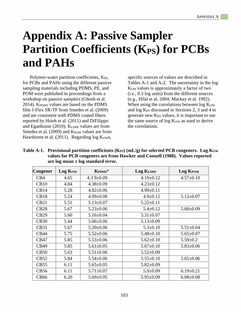
APPENDIX A
103
Appendix A: Passive Sampler
Partition Coefficients (KPS) for PCBs
and PAHs Polymer-water partition coefficients, KPS,
for PCBs and PAHs using the different passive
sampling materials including PDMS, PE, and
POM were published in proceedings from a
workshop on passive samplers (Ghosh et al.
2014). KPDMS values are based on the PDMS
film J-Flex SR-TF from Smedes et al. (2009)
and are consistent with PDMS coated fibers
reported by Hsieh et al. (2011) and DiFilippo
and Eganhouse (2010). KLDPE values are from
Smedes et al. (2009) and KPOM values are from
Hawthorne et al. (2011). Regarding log KOWs,
specific sources of values are described in
Tables A-1 and A-2. The uncertainty in the log
KOW values is approximately a factor of two
(i.e., 0.3 log units) from the different sources
(e.g., Hilal et al. 2004; Mackay et al. 1992).
When using the correlations between log KOW
and log KPS discssued in Sections 2, 3 and 4 to
generate new KPS values, it is important to use
the same source of log KOW as used to derive
the correlations.
Table A-1. Provisional partition coefficients (KPS) (mL/g) for selected PCB congeners. Log KOW
values for PCB congeners are from Hawker and Connell (1988). Values reported
are log mean ± log standard error.
Congener Log KOW KPDMSa Log KLDPE Log KPOM
CB4 4.65 4.3 9 ±0.09 4.19 ±0.12 4.57 ±0.10
CB10 4.84 4.38 ±0.09 4.23 ±0.12
CB14 5.28 4.82 ±0.06 4.99 ±0.11
CB18 5.24 4.99 ±0.08 4.9 ±0.12 5.12 ±0.07
CB21 5.51 5.13 ±0.07 5.22 ±0.11
CB28 5.67 5.23 ±0.06 5.4 ±0.12 5.68 ±0.09
CB29 5.60 5.16 ±0.04 5.31 ±0.07
CB30 5.44 5.06 ±0.06 5.13 ±0.09
CB31 5.67 5.20 ±0.06 5.3 ±0.10 5.51 ±0.04
CB44 5.75 5.52 ±0.06 5.48 ±0.10 5.65 ±0.07
CB47 5.85 5.53 ±0.06 5.62 ±0.10 5.59 ±0.2
CB49 5.85 5.61 ±0.05 5.67 ±0.10 5.83 ±0.06
CB50 5.63 5.51 ±0.06 5.52 ±0.09
CB52 5.84 5.54 ±0.06 5.55 ±0.10 5.65 ±0.06
CB55 6.11 5.65 ±0.05 5.82 ±0.09
CB56 6.11 5.71 ±0.07 5.9 ±0.09 6.19 ±0.21
CB66 6.20 5.69 ±0.05 5.95 ±0.09 6.08 ±0.08
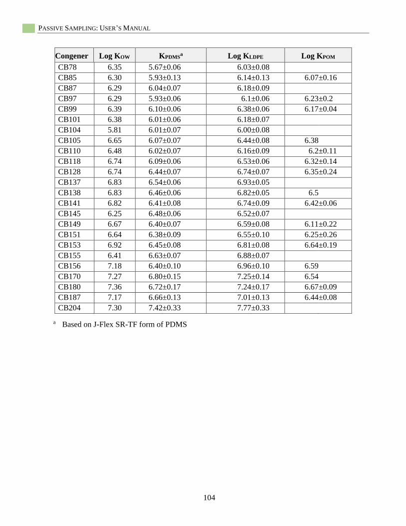
PASSIVE SAMPLING: USER’S MANUAL
104
Congener Log KOW KPDMSa Log KLDPE Log KPOM
CB78 6.35 5.67 ±0.06 6.03 ±0.08
CB85 6.30 5.93 ±0.13 6.14 ±0.13 6.07 ±0.16
CB87 6.29 6.04 ±0.07 6.18 ±0.09
CB97 6.29 5.93 ±0.06 6.1 ±0.06 6.23 ±0.2
CB99 6.39 6.10 ±0.06 6.38 ±0.06 6.17 ±0.04
CB101 6.38 6.01 ±0.06 6.18 ±0.07
CB104 5.81 6.01 ±0.07 6.00 ±0.08
CB105 6.65 6.07 ±0.07 6.44 ±0.08 6.38
CB110 6.48 6.02 ±0.07 6.16 ±0.09 6.2 ±0.11
CB118 6.74 6.09 ±0.06 6.53 ±0.06 6.32 ±0.14
CB128 6.74 6.44 ±0.07 6.74 ±0.07 6.35 ±0.24
CB137 6.83 6.54 ±0.06 6.93 ±0.05
CB138 6.83 6.46 ±0.06 6.82 ±0.05 6.5
CB141 6.82 6.41 ±0.08 6.74 ±0.09 6.42 ±0.06
CB145 6.25 6.48 ±0.06 6.52 ±0.07
CB149 6.67 6.40 ±0.07 6.59 ±0.08 6.11 ±0.22
CB151 6.64 6.38 ±0.09 6.55 ±0.10 6.25 ±0.26
CB153 6.92 6.45 ±0.08 6.81 ±0.08 6.64 ±0.19
CB155 6.41 6.63 ±0.07 6.88 ±0.07
CB156 7.18 6.40 ±0.10 6.96 ±0.10 6.59
CB170 7.27 6.80 ±0.15 7.25 ±0.14 6.54
CB180 7.36 6.72 ±0.17 7.24 ±0.17 6.67 ±0.09
CB187 7.17 6.66 ±0.13 7.01 ±0.13 6.44 ±0.08
CB204 7.30 7.42 ±0.33 7.77 ±0.33
a Based on J-Flex SR-TF form of PDMS
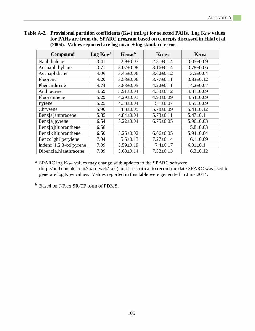
APPENDIX A
105
Table A-2. Provisional partition coefficients (KPS) (mL/g) for selected PAHs. Log KOW values
for PAHs are from the SPARC program based on concepts discussed in Hilal et al.
(2004). Values reported are log mean ± log standard error.
Compound Log KOWa KPDMS
b KLDPE KPOM
Naphthalene 3.41 2.9 ±0.07 2.81 ±0.14 3.05 ±0.09
Acenaphthylene 3.71 3.07 ±0.08 3.16 ±0.14 3.78 ±0.06
Acenaphthene 4.06 3.45 ±0.06 3.62 ±0.12 3.5 ±0.04
Fluorene 4.20 3.58 ±0.06 3.77 ±0.11 3.83 ±0.12
Phenanthrene 4.74 3.83 ±0.05 4.22 ±0.11 4.2 ±0.07
Anthracene 4.69 3.91 ±0.04 4.33 ±0.12 4.31 ±0.09
Fluoranthene 5.29 4.29 ±0.03 4.93 ±0.09 4.54 ±0.09
Pyrene 5.25 4.38 ±0.04 5.1 ±0.07 4.55 ±0.09
Chrysene 5.90 4.8 ±0.05 5.78 ±0.09 5.44 ±0.12
Benz[a]anthracene 5.85 4.84 ±0.04 5.73 ±0.11 5.47 ±0.1
Benz[a]pyrene 6.54 5.22 ±0.04 6.75 ±0.05 5.96 ±0.03
Benz[b]fluoranthene 6.58 5.8 ±0.03
Benz[k]fluoranthene 6.50 5.26 ±0.02 6.66 ±0.05 5.94 ±0.04
Benzo[ghi]perylene 7.04 5.6 ±0.13 7.27 ±0.14 6.1 ±0.09
Indeno[1,2,3-cd]pyrene 7.09 5.59 ±0.19 7.4 ±0.17 6.31 ±0.1
Dibenz[a,h]anthracene 7.39 5.68 ±0.14 7.32 ±0.13 6.3 ±0.12
a SPARC log KOW values may change with updates to the SPARC software
(http://archemcalc.com/sparc-web/calc) and it is critical to record the date SPARC was used to
generate log KOW values. Values reported in this table were generated in June 2014.
b Based on J-Flex SR-TF form of PDMS.
PASSIVE SAMPLING: USER’S MANUAL
106
The polymer-water partition coefficients
are dependent on the hydrophobicity of the
target contaminant and the passive sampling
material, but not on the amount of sorbent or its
dimensions (if equilibrium was attained). Thick
layers of sorbent may result in slow
achievement of equilibrium, and the lack of
equilibrium may be the cause of some reported
KPS that are lower than those shown in the
appendix. Some effects of the manufacture and
processing of the different polymers have been
noted particularly in PDMS (Ghosh et al.
2014). Consistent deviations of 0.1–0.3 log
units have been noted; for example, between
PDMS from different manufacturers (Smedes
et al. 2009). The larger deviations are noted for
the more hydrophobic compounds (e.g., highly
chlorinated PCBs). There are also occasional
wide variations in reported KPS for PDMS,
particularly for highly hydrophobic
compounds, which are exceedingly difficult to
measurement. Often, measurements have been
reported that are somewhat lower than for KPS
for highly hydrophobic target contaminants due
to the difficulty in achieving equilibrium with
these compounds and the potential for losses of
the contaminants to phases other than the
polymer sorbent during measurement. The
values presented here represent the best values
available, and the reader is cautioned that
attempts to refine these values for a particular
polymer sorbent and contaminants should be
undertaken only by experienced analysts
recognizing the problems involved.
There is also evidence that the values of
KPS are dependent on the temperature and
salinity of the aquatic system being measured.
Most KPS values are derived at 20–25˚C and in
deionized water. These variations are relatively
small compared to other sources of uncertainty
over the modest range of environmental
temperatures typically of interest (~5–25ºC)
and with salinities up to the salinity of
seawater. See Appendix C for further
discussion.
The estimated values of KPS are expected to
be accurate within approximately 0.3 log units
(factor of two), even for highly hydrophobic
compounds and for different sorbent sources.
The resulting error in KPS is similar in
magnitude to other environmental partition
coefficients (e.g., the octanol-water partition
coefficients (KOW). Like other environmental
sampling approaches, the uncertainty in
interstitial water or overlying water
concentrations derived from KPS values is also
likely to be dominated by the uncertainty in
whether a particular sample is representative of
environmental conditions, rather than the
specific value of KPS.
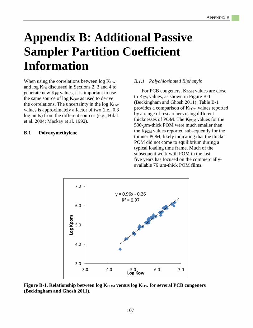
APPENDIX B
107
Appendix B: Additional Passive
Sampler Partition Coefficient
Information When using the correlations between log KOW
and log KPS discussed in Sections 2, 3 and 4 to
generate new KPS values, it is important to use
the same source of log KOW as used to derive
the correlations. The uncertainty in the log KOW
values is approximately a factor of two (i.e., 0.3
log units) from the different sources (e.g., Hilal
et al. 2004; Mackay et al. 1992).
B.1 Polyoxymethylene
B.1.1 Polychlorinated Biphenyls
For PCB congeners, KPOM values are close
to KOW values, as shown in Figure B-1
(Beckingham and Ghosh 2011). Table B-1
provides a comparison of KPOM values reported
by a range of researchers using different
thicknesses of POM. The KPOM values for the
500-µm-thick POM were much smaller than
the KPOM values reported subsequently for the
thinner POM, likely indicating that the thicker
POM did not come to equilibrium during a
typical loading time frame. Much of the
subsequent work with POM in the last
five years has focused on the commercially-
available 76 µm-thick POM films.
Figure B-1. Relationship between log KPOM versus log KOW for several PCB congeners (Beckingham and Ghosh 2011).
7.0
y = 0.96x - 0.26R² = 0.97
6.0
5.0
4.0
3.03.0 4.0 6.0 7.05.0
Log Kow
Log
Kpom
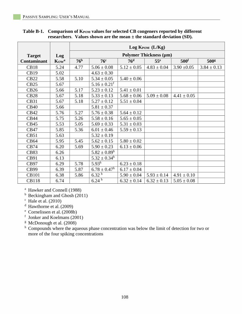
PASSIVE SAMPLING: USER’S MANUAL
108
Table B-1. Comparison of KPOM values for selected CB congeners reported by different
researchers. Values shown are the mean ± the standard deviation (SD).
Target
Contaminant
Log
KOWa
Log KPOM (L/Kg)
Polymer Thickness (µm)
76b 76c 76d 55e 500f 500g
CB18 5.24 4.77 5.06 ± 0.08 5.12 ± 0.05 4.83 ± 0.04 3.90 ±0.05 3.84 ± 0.13
CB19 5.02 4.63 ± 0.30
CB22 5.58 5.10 5.34 ± 0.05 5.40 ± 0.06
CB25 5.67 5.16 ± 0.21f
CB26 5.66 5.17 5.23 ± 0.12 5.41 ± 0.01
CB28 5.67 5.18 5.33 ± 0.13 5.68 ± 0.06 5.09 ± 0.08 4.41 ± 0.05
CB31 5.67 5.18 5.27 ± 0.12 5.51 ± 0.04
CB40 5.66 5.81 ± 0.37
CB42 5.76 5.27 5.76 ± 0.38 5.64 ± 0.12
CB44 5.75 5.26 5.58 ± 0.16 5.65 ± 0.05
CB45 5.53 5.05 5.69 ± 0.33 5.31 ± 0.03
CB47 5.85 5.36 6.01 ± 0.46 5.59 ± 0.13
CB51 5.63 5.32 ± 0.19
CB64 5.95 5.45 5.62 ± 0.15 5.80 ± 0.02
CB74 6.20 5.69 5.90 ± 0.23 6.13 ± 0.06
CB83 6.26 5.82 ± 0.89h
CB91 6.13 5.32 ± 0.34h
CB97 6.29 5.78 5.93h 6.23 ± 0.18
CB99 6.39 5.87 6.78 ± 0.47h 6.17 ± 0.04
CB101 6.38 5.86 6.32 h 5.90 ± 0.04 5.93 ± 0.14 4.91 ± 0.10
CB118 6.74 6.24 h 6.32 ± 0.14 6.32 ± 0.13 5.05 ± 0.08
a Hawker and Connell (1988)b Beckingham and Ghosh (2011) c Hale et al. (2010) d Hawthorne et al. (2009) e Cornelissen et al. (2008b)f Jonker and Koelmans (2001) g McDonough et al. (2008) h Compounds where the aqueous phase concentration was below the limit of detection for two or
more of the four spiking concentrations
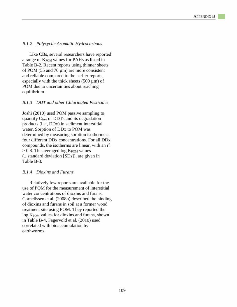
APPENDIX B
109
B.1.2 Polycyclic Aromatic Hydrocarbons
Like CBs, several researchers have reported
a range of KPOM values for PAHs as listed in
Table B-2. Recent reports using thinner sheets
of POM (55 and 76 µm) are more consistent
and reliable compared to the earlier reports,
especially with the thick sheets (500 µm) of
POM due to uncertainties about reaching
equilibrium.
B.1.3 DDT and other Chlorinated Pesticides
Joshi (2010) used POM passive sampling to
quantify Cfree of DDTs and its degradation
products (i.e., DDx) in sediment interstitial
water. Sorption of DDx to POM was
determined by measuring sorption isotherms at
four different DDx concentrations. For all DDx
compounds, the isotherms are linear, with an r2
> 0.8. The averaged log KPOM values
(± standard deviation [SDs]), are given in
Table B-3.
B.1.4 Dioxins and Furans
Relatively few reports are available for the
use of POM for the measurement of interstitial
water concentrations of dioxins and furans.
Cornelissen et al. (2008b) described the binding
of dioxins and furans in soil at a former wood
treatment site using POM. They reported the
log KPOM values for dioxins and furans, shown
in Table B-4. Fagervold et al. (2010) used
correlated with bioaccumulation by
earthworms.
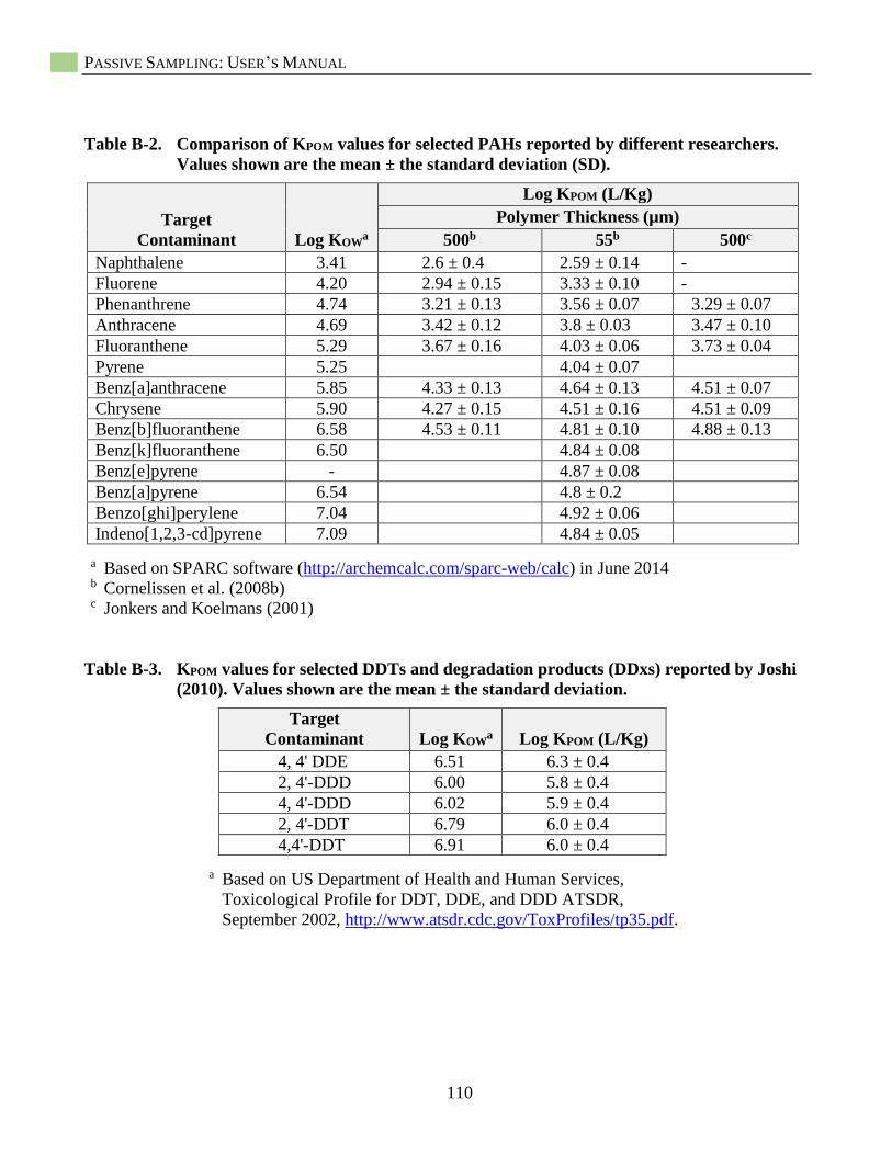
PASSIVE SAMPLING: USER’S MANUAL
110
Table B-2. Comparison of KPOM values for selected PAHs reported by different researchers.
Values shown are the mean ± the standard deviation (SD).
Target
Contaminant Log KOWa
Log KPOM (L/Kg)
Polymer Thickness (µm)
500b 55b 500c
Naphthalene 3.41 2.6 ± 0.4 2.59 ± 0.14 -
Fluorene 4.20 2.94 ± 0.15 3.33 ± 0.10 -
Phenanthrene 4.74 3.21 ± 0.13 3.56 ± 0.07 3.29 ± 0.07
Anthracene 4.69 3.42 ± 0.12 3.8 ± 0.03 3.47 ± 0.10
Fluoranthene 5.29 3.67 ± 0.16 4.03 ± 0.06 3.73 ± 0.04
Pyrene 5.25 4.04 ± 0.07
Benz[a]anthracene 5.85 4.33 ± 0.13 4.64 ± 0.13 4.51 ± 0.07
Chrysene 5.90 4.27 ± 0.15 4.51 ± 0.16 4.51 ± 0.09
Benz[b]fluoranthene 6.58 4.53 ± 0.11 4.81 ± 0.10 4.88 ± 0.13
Benz[k]fluoranthene 6.50 4.84 ± 0.08
Benz[e]pyrene - 4.87 ± 0.08
Benz[a]pyrene 6.54 4.8 ± 0.2
Benzo[ghi]perylene 7.04 4.92 ± 0.06
Indeno[1,2,3-cd]pyrene 7.09 4.84 ± 0.05
a Based on SPARC software (http://archemcalc.com/sparc-web/calc) in June 2014 b Cornelissen et al. (2008b) c Jonkers and Koelmans (2001)
Table B-3. KPOM values for selected DDTs and degradation products (DDxs) reported by Joshi
(2010). Values shown are the mean ± the standard deviation.
Target
Contaminant Log KOWa Log KPOM (L/Kg)
4, 4' DDE 6.51 6.3 ± 0.4
2, 4'-DDD 6.00 5.8 ± 0.4
4, 4'-DDD 6.02 5.9 ± 0.4
2, 4'-DDT 6.79 6.0 ± 0.4
4,4'-DDT 6.91 6.0 ± 0.4
a Based on US Department of Health and Human Services,
Toxicological Profile for DDT, DDE, and DDD ATSDR,
September 2002, http://www.atsdr.cdc.gov/ToxProfiles/tp35.pdf.

APPENDIX B
111
Table B-4. Log KPOM values for selected dioxins and furans reported by Cornelissen et al.
(2008b,c, 2010). Values shown are the mean ± the standard deviation.
Target
Contaminant Log KOWa
Log KPOM (L/Kg)
Cornelissen et
al. (2008b)
Cornelissen et al.
(2008c, 2010)
2-MCDF 5.3
2,8-DCDF 5.5 5.32 ± 0.09b
1,6-DCDD 6.2 5.24 ± 0.07b
2,4,8-TCDF 6.9 5.65 ± 0.09b
1,3,6,8-TCDF 6.5 5.78 ± 0.35b
2,3,7,8-TCDF 6.41 5.74 b
2,3,7,8-TCDD 7.05 5.86 b
1,3,6,8-TCDD 6.8 5.79 ± 0.35b
1,2,3,7,8-PCDF 6.74 5.87 b
1,2,3,7,8-PCDD 7.06 6.00 b
1,2,3,8,9-PCDF 7.4 5.99 ± 0.43b
2,3,4,7,8-PCDF 6.8 5.90 b
1,2,3,4,6,9-HCDD 7.8 6.40 ± 0.32b
1,2,3,4,7,8-HCDF 7.46 6.00 b
1,2,3,4,7,8-HCDD 7.93 6.10 b
1,2,3,6,7,8-HCDF 7.56 6.01 b
1,2,3,6,7,8-HCDD 7.93 6.11 b
1,2,3,7,8,9-HCDF 7.44 6.06 b
1,2,3,7,8,9-HCDD 7.91 6.09 b
2,3,4,6,7,8-HCDF 7.43 6.03 b
1,2,3,4,6,7,8-HCDF 7.81 6.12 b
1,2,3,4,6,7,8-HCDD 8.42 6.21 b
1,2,3,4,6,7,9-HCDD 8 6.30 ± 0.29b
1,2,3,4,7,8,9-HCDF 7.92 6.17 b
OCDF 8.43 6.33c 6.26 b
OCDD 8.85 6.46c 6.30 b
a Based on Sacan et al. (2005) b Measured values c Extrapolated values
B.2 Polydimethylsiloxane
B.2.1 Polychlorinated Biphenyls and
Polycyclic Aromatic Hydrocarbons
Tables B-5 and B-6 report alternative KPDMS
values for PCBs and PAHs. Other alternative
sources of KPDMS values not explicitly reported
here include Reible and Lotufo (2012), Reible
et al. (2012) and DiFilippo and Eaganhouse
(2010).
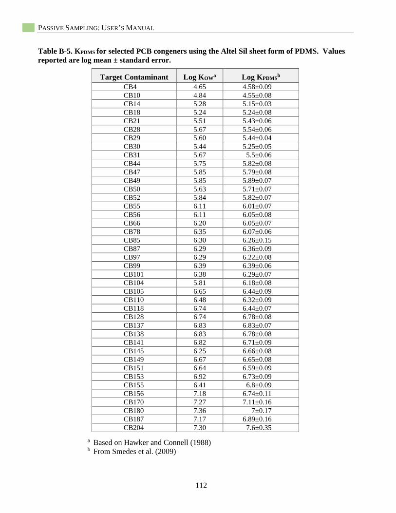
PASSIVE SAMPLING: USER’S MANUAL
112
Table B-5. KPDMS for selected PCB congeners using the Altel Sil sheet form of PDMS. Values
reported are log mean ± standard error.
Target Contaminant Log KOWa Log KPDMS
b
CB4 4.65 4.58 ±0.09
CB10 4.84 4.55 ±0.08
CB14 5.28 5.15 ±0.03
CB18 5.24 5.24 ±0.08
CB21 5.51 5.43 ±0.06
CB28 5.67 5.54 ±0.06
CB29 5.60 5.44 ±0.04
CB30 5.44 5.25 ±0.05
CB31 5.67 5.5 ±0.06
CB44 5.75 5.82 ±0.08
CB47 5.85 5.79 ±0.08
CB49 5.85 5.89 ±0.07
CB50 5.63 5.71 ±0.07
CB52 5.84 5.82 ±0.07
CB55 6.11 6.01 ±0.07
CB56 6.11 6.05 ±0.08
CB66 6.20 6.05 ±0.07
CB78 6.35 6.07 ±0.06
CB85 6.30 6.26 ±0.15
CB87 6.29 6.36 ±0.09
CB97 6.29 6.22 ±0.08
CB99 6.39 6.39 ±0.06
CB101 6.38 6.29 ±0.07
CB104 5.81 6.18 ±0.08
CB105 6.65 6.44 ±0.09
CB110 6.48 6.32 ±0.09
CB118 6.74 6.44 ±0.07
CB128 6.74 6.78 ±0.08
CB137 6.83 6.83 ±0.07
CB138 6.83 6.78 ±0.08
CB141 6.82 6.71 ±0.09
CB145 6.25 6.66 ±0.08
CB149 6.67 6.65 ±0.08
CB151 6.64 6.59 ±0.09
CB153 6.92 6.73 ±0.09
CB155 6.41 6.8 ±0.09
CB156 7.18 6.74 ±0.11
CB170 7.27 7.11 ±0.16
CB180 7.36 7 ±0.17
CB187 7.17 6.89 ±0.16
CB204 7.30 7.6 ±0.35
a Based on Hawker and Connell (1988) b From Smedes et al. (2009)
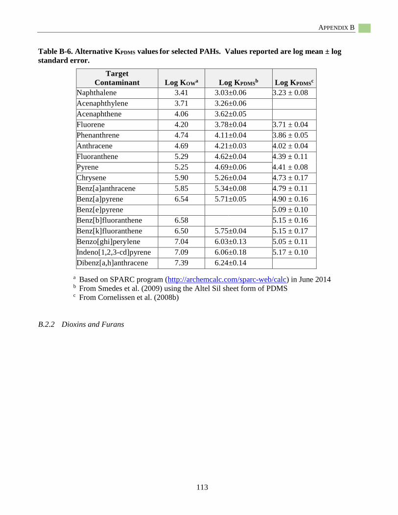
APPENDIX B
113
Table B-6. Alternative KPDMS values for selected PAHs. Values reported are log mean ± log
standard error.
Target
Contaminant Log KOWa Log KPDMS
b Log KPDMSc
Naphthalene 3.41 3.03 ±0.06 3.23 ± 0.08
Acenaphthylene 3.71 3.26 ±0.06
Acenaphthene 4.06 3.62 ±0.05
Fluorene 4.20 3.78 ±0.04 3.71 ± 0.04
Phenanthrene 4.74 4.11 ±0.04 3.86 ± 0.05
Anthracene 4.69 4.21 ±0.03 4.02 ± 0.04
Fluoranthene 5.29 4.62 ±0.04 4.39 ± 0.11
Pyrene 5.25 4.69 ±0.06 4.41 ± 0.08
Chrysene 5.90 5.26 ±0.04 4.73 ± 0.17
Benz[a]anthracene 5.85 5.34 ±0.08 4.79 ± 0.11
Benz[a]pyrene 6.54 5.71 ±0.05 4.90 ± 0.16
Benz[e]pyrene 5.09 ± 0.10
Benz[b]fluoranthene 6.58 5.15 ± 0.16
Benz[k]fluoranthene 6.50 5.75 ±0.04 5.15 ± 0.17
Benzo[ghi]perylene 7.04 6.03 ±0.13 5.05 ± 0.11
Indeno[1,2,3-cd]pyrene 7.09 6.06 ±0.18 5.17 ± 0.10
Dibenz[a,h]anthracene 7.39 6.24 ±0.14
a Based on SPARC program (http://archemcalc.com/sparc-web/calc) in June 2014 b From Smedes et al. (2009) using the Altel Sil sheet form of PDMS c From Cornelissen et al. (2008b)
B.2.2 Dioxins and Furans
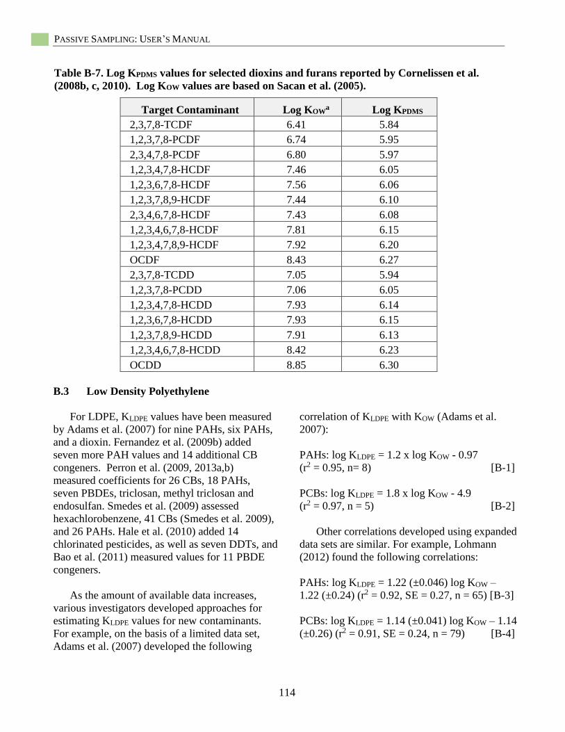
PASSIVE SAMPLING: USER’S MANUAL
114
Table B-7. Log KPDMS values for selected dioxins and furans reported by Cornelissen et al.
(2008b, c, 2010). Log KOW values are based on Sacan et al. (2005).
Target Contaminant Log KOWa Log KPDMS
2,3,7,8-TCDF 6.41 5.84
1,2,3,7,8-PCDF 6.74 5.95
2,3,4,7,8-PCDF 6.80 5.97
1,2,3,4,7,8-HCDF 7.46 6.05
1,2,3,6,7,8-HCDF 7.56 6.06
1,2,3,7,8,9-HCDF 7.44 6.10
2,3,4,6,7,8-HCDF 7.43 6.08
1,2,3,4,6,7,8-HCDF 7.81 6.15
1,2,3,4,7,8,9-HCDF 7.92 6.20
OCDF 8.43 6.27
2,3,7,8-TCDD 7.05 5.94
1,2,3,7,8-PCDD 7.06 6.05
1,2,3,4,7,8-HCDD 7.93 6.14
1,2,3,6,7,8-HCDD 7.93 6.15
1,2,3,7,8,9-HCDD 7.91 6.13
1,2,3,4,6,7,8-HCDD 8.42 6.23
OCDD 8.85 6.30
B.3 Low Density Polyethylene
For LDPE, KLDPE values have been measured
by Adams et al. (2007) for nine PAHs, six PAHs,
and a dioxin. Fernandez et al. (2009b) added
seven more PAH values and 14 additional CB
congeners. Perron et al. (2009, 2013a,b)
measured coefficients for 26 CBs, 18 PAHs,
seven PBDEs, triclosan, methyl triclosan and
endosulfan. Smedes et al. (2009) assessed
hexachlorobenzene, 41 CBs (Smedes et al. 2009),
and 26 PAHs. Hale et al. (2010) added 14
chlorinated pesticides, as well as seven DDTs, and
Bao et al. (2011) measured values for 11 PBDE
congeners.
As the amount of available data increases,
various investigators developed approaches for
estimating KLDPE values for new contaminants.
For example, on the basis of a limited data set,
Adams et al. (2007) developed the following
correlation of KLDPE with KOW (Adams et al.
2007):
PAHs: log KLDPE = 1.2 x log KOW - 0.97
(r2 = 0.95, n= 8) [B-1]
PCBs: log KLDPE = 1.8 x log KOW - 4.9
(r2 = 0.97, n = 5) [B-2]
Other correlations developed using expanded
data sets are similar. For example, Lohmann
(2012) found the following correlations:
PAHs: log KLDPE = 1.22 (±0.046) log KOW –
1.22 (±0.24) (r2 = 0.92, SE = 0.27, n = 65) [B-3]
PCBs: log KLDPE = 1.14 (±0.041) log KOW – 1.14
(±0.26) (r2 = 0.91, SE = 0.24, n = 79) [B-4]

APPENDIX C
115
Appendix C: Effects of Temperature
and Salinity on Polymer-Water
Partition Coefficients Passive samplers may find use in diverse
environments and at different times of year, so
one may expect that the data will reflect
polymer-water partitioning at temperatures
between 0 and 30°C and at salinities varying
from 0‰ to 35‰. Hence, one may need to
adjust KPS values to reflect site conditions
when the passive sampling is performed.
This discussion is focused primarily on low
density polyethylene, although the
experimental data for LDPE are limited it is
more extensive than the other polymers. For
example, Reible and Lotufo (2012) and Reible
et al. (2012) reported for two PDMS SPME
fibers (i.e., Fiberguide 230/210 and Polymicro
Technologies Inc. 170/110) that temperatures
ranging from 4 to 25˚C had little effect on
KPDMS values. Recently, Jonker et al. (2015)
investigated the effects of temperature (4 to 30
˚C) and salinity (0 to 36 ‰) on PDMS film
(Alteweb AlteSil 500 µm thick) partition
coefficients. They found significant effects
caused by temperature and salinity resulting in
reductions in Cfree for several PCBs and PAHs,
on average, by a factor of 1.6. The effect was
most significant for higher KOW chemicals.
Jonker et al. (2015) provide an equation for
adjusting the PDMS partition coefficient to
account for the effects of temperature and
salinity.
For LDPE, work has been performed to
quantify the effects of temperature on KLDPE
values. First, the data indicate that temperature
affects KLDPE chiefly through the target
contaminant's excess enthalpy of solution in
water, since the excess enthalpy of solution of
hydrophobic compounds in hydrophobic media
is generally small (Schwarzenbach et al. 2003).
Consequently, the temperature effect can be
estimated using:
KLDPE (T) = KLDPE(Tref) * exp [(∆HE/R)(1/T –
1/ Tref)] [C-1]
where: KLDPE (T) is the polyethylene-water
partition coefficient at temperature, T, KLDPE
(Tref) is the polyethylene-water partition
coefficient at some reference temperature
(e.g., 25°C), ∆HE is the excess enthalpy of
solution for the target compound dissolved in
water, R is the gas constant (8.31 J/mol K), T is
the environmental temperature of interest (in
K), and Tref is the (laboratory) reference
temperature at which the KLDPE has been
measured.
In tests of this approach, Adams et al.
(2007) found that the temperature dependencies
of KLDPE values for phenanthrene, pyrene, and
2, 2', 5, 5'-tetrachlorobiphenyl (CB52) were
consistent with the use of reported ∆HE values
(Haftka et al. 2010; Shiu and Ma 2000). For
example, using an excess enthalpy of aqueous
solution for 2,2',5,5'-tetrachlorobiphenyl of +16
kJ/mol, one estimates that the reported KLDPE
(23oC) of log 5.4 (Hafka et al. 2010, Shiu and
Ma 2000) should be increased by a factor of 1.6
for the case of a freshwater lake at 4°C to
KLDPE (4°C) of log 5.6. The measured value
was log 5.5 (Adams et al. 2007).
In order to treat the effects of dissolved
salts (i.e., seawater), the data also indicate that
PASSIVE SAMPLING: USER’S MANUAL
116
one can use the target contaminant's Setchenow
constant:
KLDPE,salt = KLDPE * 10 Ks * [salt] [C-2]
where, KS is the Setschenow constant (1/M),
and [salt] is the salt concentration (M).
For example, assuming that KS is 0.28 M-1
for phenanthrene and a measured KLDPE of log
4.3 for this PAH, for an 0.5 M NaCl water
solution (comparable to full-strength seawater),
one finds that the KLDPE,salt is expected to be
1.07 times greater than KLDPE for phenanthrene.
Experimental measurements confirmed this
expectation (Adams et al. 2007). Using this
approach, for the case of full-strength seawater,
the dissolved salt would cause a small increase
in the KLDPE (phenanthrene) of about 40% to
log 4.4.
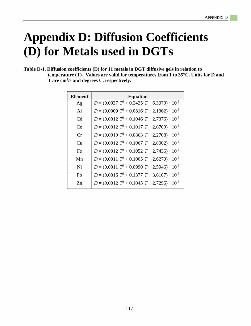
APPENDIX D
117
Appendix D: Diffusion Coefficients
(D) for Metals used in DGTs
Table D-1. Diffusion coefficients (D) for 11 metals in DGT diffusive gels in relation to
temperature (T). Values are valid for temperatures from 1 to 35°C. Units for D and
T are cm2/s and degrees C, respectively.
Element Equation
Ag D = (0.0027·T2 + 0.2425·T + 6.3370) · 10-6
Al D = (0.0009·T2 + 0.0816·T + 2.1362) · 10-6
Cd D = (0.0012·T2 + 0.1046·T + 2.7376) · 10-6
Co D = (0.0012·T2 + 0.1017·T + 2.6709) · 10-6
Cr D = (0.0010·T2 + 0.0863·T + 2.2708) · 10-6
Cu D = (0.0012·T2 + 0.1067·T + 2.8002) · 10-6
Fe D = (0.0012·T2 + 0.1052·T + 2.7436) · 10-6
Mn D = (0.0011·T2 + 0.1005·T + 2.6270) · 10-6
Ni D = (0.0011·T2 + 0.0990·T + 2.5946) · 10-6
Pb D = (0.0016·T2 + 0.1377·T + 3.6107) · 10-6
Zn D = (0.0012·T2 + 0.1045·T + 2.7296) · 10-6
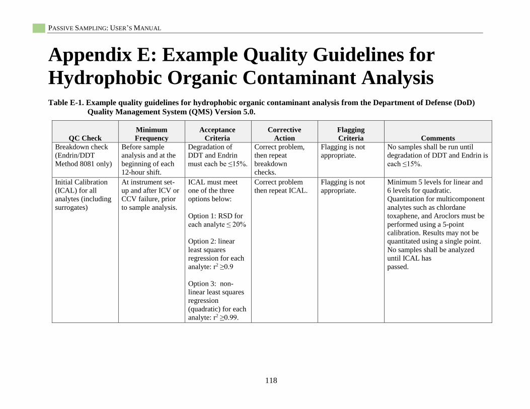
PASSIVE SAMPLING: USER’S MANUAL
118
Appendix E: Example Quality Guidelines for
Hydrophobic Organic Contaminant Analysis Table E-1. Example quality guidelines for hydrophobic organic contaminant analysis from the Department of Defense (DoD)
Quality Management System (QMS) Version 5.0.
QC Check
Minimum
Frequency
Acceptance
Criteria
Corrective
Action
Flagging
Criteria Comments
Breakdown check
(Endrin/DDT
Method 8081 only)
Before sample
analysis and at the
beginning of each
12-hour shift.
Degradation of
DDT and Endrin
must each be ≤15%.
Correct problem,
then repeat
breakdown
checks.
Flagging is not
appropriate.
No samples shall be run until
degradation of DDT and Endrin is
each ≤15%.
Initial Calibration
(ICAL) for all
analytes (including
surrogates)
At instrument set-
up and after ICV or
CCV failure, prior
to sample analysis.
ICAL must meet
one of the three
options below:
Option 1: RSD for
each analyte ≤ 20%
Option 2: linear
least squares
regression for each
analyte: r2 ≥0.9
Option 3: non-
linear least squares
regression
(quadratic) for each
analyte: r2 ≥0.99.
Correct problem
then repeat ICAL.
Flagging is not
appropriate.
Minimum 5 levels for linear and
6 levels for quadratic.
Quantitation for multicomponent
analytes such as chlordane
toxaphene, and Aroclors must be
performed using a 5-point
calibration. Results may not be
quantitated using a single point.
No samples shall be analyzed
until ICAL has
passed.

APPENDIX E
119
QC Check
Minimum
Frequency
Acceptance
Criteria
Corrective
Action
Flagging
Criteria Comments
Retention Time
window position
establishment
Once per ICAL and
at the beginning of
the analytical
sequence.
Position shall be set
using the midpoint
standard of the
ICAL curve when
ICAL is performed.
On days when
ICAL is not
performed, the
initial CCV is used.
NA. NA. Calculated for each analyte and
surrogate.
Retention Time
(RT) window width
At method set-up
and after major
maintenance
(e.g., column
change).
RT width is ± 3
times standard
deviation for each
analyte RT from the
72-hour study.
NA. NA. Calculated for each analyte and
surrogate.
Initial Calibration
Verification (ICV)
Once after each
ICAL, analysis of a
second source
standard prior to
sample analysis.
All reported
analytes within
established RT
windows.
All reported
analytes within ±
20% of true value.
Correct problem,
rerun ICV. If that
fails, repeat ICAL.
Flagging is not
appropriate.
No samples shall be analyzed
until calibration has been verified
with a second source.
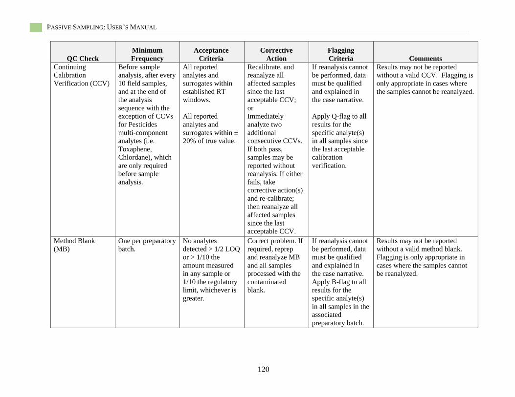
PASSIVE SAMPLING: USER’S MANUAL
120
QC Check
Minimum
Frequency
Acceptance
Criteria
Corrective
Action
Flagging
Criteria Comments
Continuing
Calibration
Verification (CCV)
Before sample
analysis, after every
10 field samples,
and at the end of
the analysis
sequence with the
exception of CCVs
for Pesticides
multi-component
analytes (i.e.
Toxaphene,
Chlordane), which
are only required
before sample
analysis.
All reported
analytes and
surrogates within
established RT
windows.
All reported
analytes and
surrogates within ±
20% of true value.
Recalibrate, and
reanalyze all
affected samples
since the last
acceptable CCV;
or
Immediately
analyze two
additional
consecutive CCVs.
If both pass,
samples may be
reported without
reanalysis. If either
fails, take
corrective action(s)
and re-calibrate;
then reanalyze all
affected samples
since the last
acceptable CCV.
If reanalysis cannot
be performed, data
must be qualified
and explained in
the case narrative.
Apply Q-flag to all
results for the
specific analyte(s)
in all samples since
the last acceptable
calibration
verification.
Results may not be reported
without a valid CCV. Flagging is
only appropriate in cases where
the samples cannot be reanalyzed.
Method Blank
(MB)
One per preparatory
batch.
No analytes
detected > 1/2 LOQ
or > 1/10 the
amount measured
in any sample or
1/10 the regulatory
limit, whichever is
greater.
Correct problem. If
required, reprep
and reanalyze MB
and all samples
processed with the
contaminated
blank.
If reanalysis cannot
be performed, data
must be qualified
and explained in
the case narrative.
Apply B-flag to all
results for the
specific analyte(s)
in all samples in the
associated
preparatory batch.
Results may not be reported
without a valid method blank.
Flagging is only appropriate in
cases where the samples cannot
be reanalyzed.
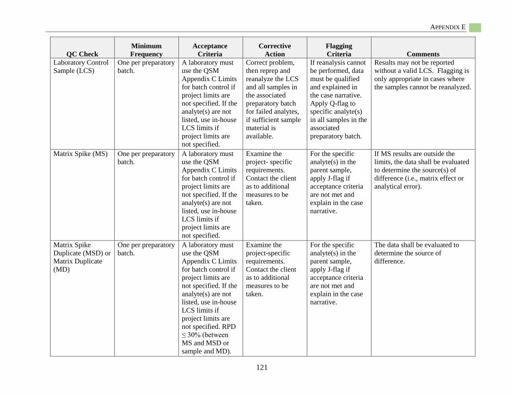
APPENDIX E
121
QC Check
Minimum
Frequency
Acceptance
Criteria
Corrective
Action
Flagging
Criteria Comments
Laboratory Control
Sample (LCS)
One per preparatory
batch.
A laboratory must
use the QSM
Appendix C Limits
for batch control if
project limits are
not specified. If the
analyte(s) are not
listed, use in-house
LCS limits if
project limits are
not specified.
Correct problem,
then reprep and
reanalyze the LCS
and all samples in
the associated
preparatory batch
for failed analytes,
if sufficient sample
material is
available.
If reanalysis cannot
be performed, data
must be qualified
and explained in
the case narrative.
Apply Q-flag to
specific analyte(s)
in all samples in the
associated
preparatory batch.
Results may not be reported
without a valid LCS. Flagging is
only appropriate in cases where
the samples cannot be reanalyzed.
Matrix Spike (MS) One per preparatory
batch.
A laboratory must
use the QSM
Appendix C Limits
for batch control if
project limits are
not specified. If the
analyte(s) are not
listed, use in-house
LCS limits if
project limits are
not specified.
Examine the
project- specific
requirements.
Contact the client
as to additional
measures to be
taken.
For the specific
analyte(s) in the
parent sample,
apply J-flag if
acceptance criteria
are not met and
explain in the case
narrative.
If MS results are outside the
limits, the data shall be evaluated
to determine the source(s) of
difference (i.e., matrix effect or
analytical error).
Matrix Spike
Duplicate (MSD) or
Matrix Duplicate
(MD)
One per preparatory
batch.
A laboratory must
use the QSM
Appendix C Limits
for batch control if
project limits are
not specified. If the
analyte(s) are not
listed, use in-house
LCS limits if
project limits are
not specified. RPD
≤ 30% (between
MS and MSD or
sample and MD).
Examine the
project-specific
requirements.
Contact the client
as to additional
measures to be
taken.
For the specific
analyte(s) in the
parent sample,
apply J-flag if
acceptance criteria
are not met and
explain in the case
narrative.
The data shall be evaluated to
determine the source of
difference.
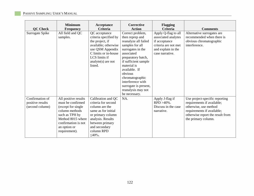
PASSIVE SAMPLING: USER’S MANUAL
122
QC Check
Minimum
Frequency
Acceptance
Criteria
Corrective
Action
Flagging
Criteria Comments
Surrogate Spike All field and QC
samples.
QC acceptance
criteria specified by
the project, if
available; otherwise
use QSM Appendix
C limits or in-house
LCS limits if
analyte(s) are not
listed.
Correct problem,
then reprep and
reanalyze all failed
samples for all
surrogates in the
associated
preparatory batch,
if sufficient sample
material is
available. If
obvious
chromatographic
interference with
surrogate is present,
reanalysis may not
be necessary.
Apply Q-flag to all
associated analytes
if acceptance
criteria are not met
and explain in the
case narrative.
Alternative surrogates are
recommended when there is
obvious chromatographic
interference.
Confirmation of
positive results
(second column)
All positive results
must be confirmed
(except for single
column methods
such as TPH by
Method 8015 where
confirmation is not
an option or
requirement).
Calibration and QC
criteria for second
column are the
same as for initial
or primary column
analysis. Results
between primary
and secondary
column RPD
≤40%.
NA. Apply J-flag if
RPD >40%.
Discuss in the case
narrative.
Use project-specific reporting
requirements if available;
otherwise, use method
requirements if available;
otherwise report the result from
the primary column.
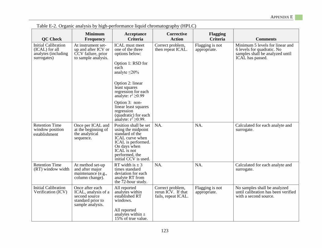
APPENDIX E
123
Table E-2. Organic analysis by high-performance liquid chromatography (HPLC)
QC Check
Minimum
Frequency
Acceptance
Criteria
Corrective
Action
Flagging
Criteria Comments
Initial Calibration (ICAL) for all analytes (including surrogates)
At instrument set-up and after ICV or CCV failure, prior to sample analysis.
ICAL must meet one of the three options below:
Option 1: RSD for each analyte ≤20%
Option 2: linear least squares regression for each analyte: r2 ≥0.99
Option 3: non-linear least squares regression (quadratic) for each analyte: r2 ≥0.99.
Correct problem, then repeat ICAL.
Flagging is not appropriate.
Minimum 5 levels for linear and 6 levels for quadratic. No samples shall be analyzed until ICAL has passed.
Retention Time window position establishment
Once per ICAL and at the beginning of the analytical sequence.
Position shall be set using the midpoint standard of the ICAL curve when ICAL is performed. On days when ICAL is not performed, the initial CCV is used.
NA. NA. Calculated for each analyte and surrogate.
Retention Time (RT) window width
At method set-up and after major maintenance (e.g., column change).
RT width is ± 3 times standard deviation for each analyte RT from the 72-hour study.
NA. NA. Calculated for each analyte and surrogate.
Initial Calibration Verification (ICV)
Once after each ICAL, analysis of a second source standard prior to sample analysis.
All reported analytes within established RT windows.
All reported analytes within ± 15% of true value.
Correct problem, rerun ICV. If that fails, repeat ICAL.
Flagging is not appropriate.
No samples shall be analyzed until calibration has been verified with a second source.
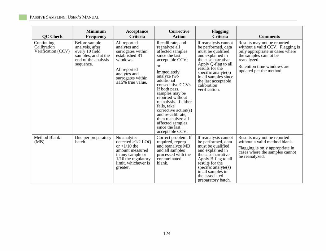
PASSIVE SAMPLING: USER’S MANUAL
124
QC Check
Minimum
Frequency
Acceptance
Criteria
Corrective
Action
Flagging
Criteria Comments
Continuing Calibration Verification (CCV)
Before sample analysis, after every 10 field samples, and at the end of the analysis sequence.
All reported analytes and surrogates within established RT windows.
All reported analytes and surrogates within ±15% true value.
Recalibrate, and reanalyze all affected samples since the last acceptable CCV;
or
Immediately analyze two additional consecutive CCVs. If both pass, samples may be reported without reanalysis. If either fails, take corrective action(s) and re-calibrate; then reanalyze all affected samples since the last acceptable CCV.
If reanalysis cannot be performed, data must be qualified and explained in the case narrative. Apply Q-flag to all results for the specific analyte(s) in all samples since the last acceptable calibration verification.
Results may not be reported without a valid CCV. Flagging is only appropriate in cases where the samples cannot be reanalyzed.
Retention time windows are updated per the method.
Method Blank (MB)
One per preparatory batch.
No analytes detected >1/2 LOQ or >1/10 the amount measured in any sample or 1/10 the regulatory limit, whichever is greater.
Correct problem. If required, reprep and reanalyze MB and all samples processed with the contaminated blank.
If reanalysis cannot be performed, data must be qualified and explained in the case narrative. Apply B-flag to all results for the specific analyte(s) in all samples in the associated preparatory batch.
Results may not be reported without a valid method blank.
Flagging is only appropriate in cases where the samples cannot be reanalyzed.
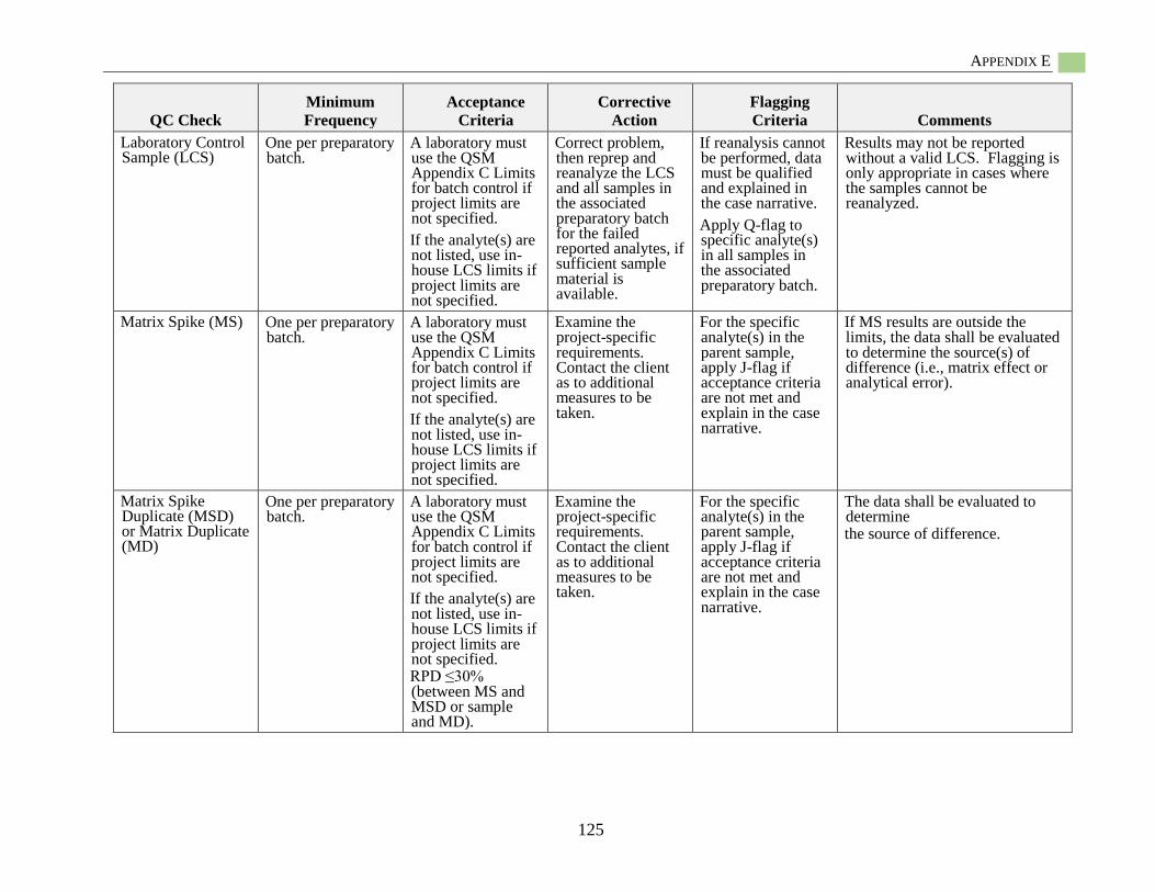
APPENDIX E
125
QC Check
Minimum
Frequency
Acceptance
Criteria
Corrective
Action
Flagging
Criteria Comments
Laboratory Control Sample (LCS)
One per preparatory batch.
A laboratory must use the QSM Appendix C Limits for batch control if project limits are not specified.
If the analyte(s) are not listed, use in-house LCS limits if project limits are not specified.
Correct problem, then reprep and reanalyze the LCS and all samples in the associated preparatory batch for the failed reported analytes, if sufficient sample material is available.
If reanalysis cannot be performed, data must be qualified and explained in the case narrative.
Apply Q-flag to specific analyte(s) in all samples in the associated preparatory batch.
Results may not be reported without a valid LCS. Flagging is only appropriate in cases where the samples cannot be reanalyzed.
Matrix Spike (MS) One per preparatory batch.
A laboratory must use the QSM Appendix C Limits for batch control if project limits are not specified.
If the analyte(s) are not listed, use in-house LCS limits if project limits are not specified.
Examine the project-specific requirements. Contact the client as to additional measures to be taken.
For the specific analyte(s) in the parent sample, apply J-flag if acceptance criteria are not met and explain in the case narrative.
If MS results are outside the limits, the data shall be evaluated to determine the source(s) of difference (i.e., matrix effect or analytical error).
Matrix Spike Duplicate (MSD) or Matrix Duplicate (MD)
One per preparatory batch.
A laboratory must use the QSM Appendix C Limits for batch control if project limits are not specified.
If the analyte(s) are not listed, use in-house LCS limits if project limits are not specified. RPD ≤30% (between MS and MSD or sample and MD).
Examine the project-specific requirements. Contact the client as to additional measures to be taken.
For the specific analyte(s) in the parent sample, apply J-flag if acceptance criteria are not met and explain in the case narrative.
The data shall be evaluated to determine the source of difference.
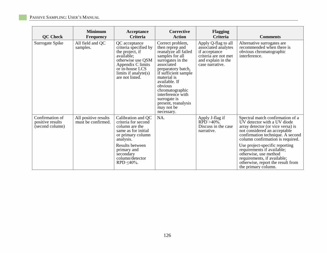
PASSIVE SAMPLING: USER’S MANUAL
126
QC Check
Minimum
Frequency
Acceptance
Criteria
Corrective
Action
Flagging
Criteria Comments
Surrogate Spike All field and QC samples.
QC acceptance criteria specified by the project, if available; otherwise use QSM Appendix C limits or in-house LCS limits if analyte(s) are not listed.
Correct problem, then reprep and reanalyze all failed samples for all surrogates in the associated preparatory batch, if sufficient sample material is available. If obvious chromatographic interference with surrogate is present, reanalysis may not be necessary.
Apply Q-flag to all associated analytes if acceptance criteria are not met and explain in the case narrative.
Alternative surrogates are recommended when there is obvious chromatographic interference.
Confirmation of positive results (second column)
All positive results must be confirmed.
Calibration and QC criteria for second column are the same as for initial or primary column analysis.
Results between primary and secondary column/detector RPD ≤40%.
NA. Apply J-flag if RPD >40%. Discuss in the case narrative.
Spectral match confirmation of a UV detector with a UV diode array detector (or vice versa) is not considered an acceptable confirmation technique. A second column confirmation is required.
Use project-specific reporting requirements if available; otherwise, use method requirements, if available; otherwise, report the result from the primary column.

APPENDIX F
127
Appendix F: Case Studies
This appendix provides a set of six case studies
illustrating the use of passive sampling at
contaminated sediment sites.
Case Study 1: Lower Grasse River,
New York, USA
Background
Target Contaminants:
Polychlorinated biphenyls (PCBs)
Passive Sampler:
Polyoxymethylene (POM)
Site Narrative
According to Alcoa (2001), the main source
of PCBs to the water column in the lower Grasse
River in New York (USA) is diffusive flux from
the sediment bed. PCBs desorb from the
sediment, diffuse through interstitial water,
and migrate past the sediment/water interface
and into the overlying water. It has been
determined that the mass transfer of CBs into
the water column is twice as high during the
summer months than during the rest of the year
(Alcoa 2001).
In 2006, activated carbon (AC) was amended
to river sediments over a 2000-m2 area of the
lower Grasse River where total concentrations of
PCBs in surficial sediments were 2 to 4 μg/g dry
wt. A comprehensive monitoring program was
established to track the following changes in
bioavailability over time: (1) measurements of
AC distributions and (2) bioaccumulation of
PCBs by freshwater invertebrates. POM samplers
were deployed in field to measure PCB Cfree
in surface waters and interstitial waters
(Beckingham and Ghosh 2013).
Project Objectives
To compare passive sampler measurements
to changes in bioavailability measured with
sediment invertebrate bioaccumulation tests
(Beckingham and Ghosh 2013).
Deployment and Retrieval of POM Samplers
POM strips obtained from the Norwegian
Geotechnical Institute were cut to 55 μm thick,
cleaned via Soxhlet extraction with hexane for
12 hours, air-dried in a fume hood, cut down to
0.2-g strips, and stored in a glass jar until
deployment. The strips were attached with plastic
wire ties to a rope and wire basket (Figure F-1)
used for the bioaccumulation tests and positioned
in duplicate on the surficial sediment (0 cm,
bottom of the basket) and at 7.5, 30, and 60 cm
in the water column above the sediment surface.
The strips were retrieved after 14 days, rinsed
with site water, and stored in glass vials at 4°C.
Baseline measurements were taken in 2006,
followed by continued monitoring events in
2007, 2008 and 2009. POM was deployed at an
untreated background site and at an AC treated
site in 2006 and 2007; POM deployments were
extended to two additional sites in both areas in
2008 and 2009 (Beckingham and Ghosh 2013).

PASSIVE SAMPLING: USER’S MANUAL
128
Figure F-1. Deployment of POM strips in
the field. POM strips were wire-tied to the
basket and rope (Beckingham and Ghosh
2013).
Analytical Methods
The following is taken from Beckingham and
Ghosh (2013). To process POM for CB analysis,
strips were wiped clean and then extracted by
agitating in 12 mL glass vials on a horizontal
shaker with 10 mL hexane for five days
(Cornelissen et al. 2008). Extracts were then
spiked with surrogate standards (PCB congeners
CB14 and CB65), concentrated to 1 mL, and
cleaned by column chromatography. Columns
consisted of disposable glass Pasteur pipettes
(14.5 cm length × 6 mm diameter) plugged with
glass wool containing ~0.7 g of 3% deactivated
silica gel, and the CBs were eluted with 8 mL of
hexane. Internal standards were added (CB30 and
CB204), and CBs (90 individual and co-eluting
congener peaks) were analyzed by gas
chromatography with electron capture detection
(GC-ECD) following a modified EPA method
described in Ghosh et al. (2003). Surrogate
compound recovery was within acceptable
criteria of 100 ± 30%. However, an additional
extraction with hexane:acetone (1:1,vol) of
several POM strips found that ~8%–20% of total
CBs remained after the initial 5-day hexane
extraction. All data herein show results that have
not been corrected to compensate for this
systematic error. POM in batch tests was
extracted with the same method to enable
comparison to the field data. Aqueous
concentrations were calculated according to
Equation 8-1:
POM
POM
freeK
CC
where, Cfree is the freely dissolved concentration,
CPOM is the amount accumulated in the polymer
at equilibrium, and KPOM is the polymer-water
distribution coefficient.
Results
Results showed that sediments treated with
AC behaved as a sink for CBs in the water
column (Figure F-2); CB concentrations were
lower at the sediment/water interface in treated
areas (2007–2009) than in background sites,
and lower than concentrations at treated areas
in 2006, prior to AC amendment. In general,
reduced uptake of PCB Cfree homologs di-
through penta- in POM passive samplers
correlated with reduced uptake in invertebrates
(Figure F-3) (Beckingham and Ghosh 2013).
The study ultimately showed that POM
passive samplers can be effective tools for
monitoring changes in PCB Cfree, and that the
bioavailability of PCBs is significantly reduced
with the addition of AC (Beckingham and
Ghosh 2013).

APPENDIX F
129
Figure F-2. Gradient of total PCB Cfree from the sediment/water
interface into the water column in untreated (A) and AC treated
(B) areas (Beckingham and Ghosh 2013).
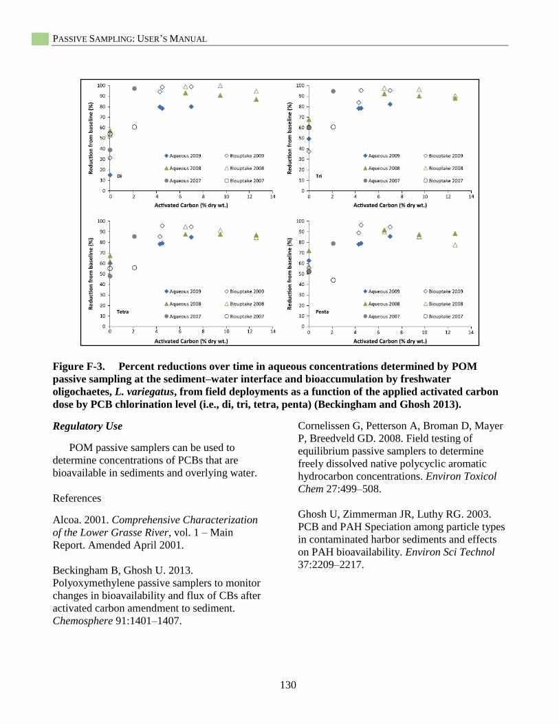
PASSIVE SAMPLING: USER’S MANUAL
130
Figure F-3. Percent reductions over time in aqueous concentrations determined by POM
passive sampling at the sediment–water interface and bioaccumulation by freshwater
oligochaetes, L. variegatus, from field deployments as a function of the applied activated carbon
dose by PCB chlorination level (i.e., di, tri, tetra, penta) (Beckingham and Ghosh 2013).
Regulatory Use
POM passive samplers can be used to
determine concentrations of PCBs that are
bioavailable in sediments and overlying water.
References
Alcoa. 2001. Comprehensive Characterization
of the Lower Grasse River, vol. 1 – Main
Report. Amended April 2001.
Beckingham B, Ghosh U. 2013.
Polyoxymethylene passive samplers to monitor
changes in bioavailability and flux of CBs after
activated carbon amendment to sediment.
Chemosphere 91:1401–1407.
Cornelissen G, Petterson A, Broman D, Mayer
P, Breedveld GD. 2008. Field testing of
equilibrium passive samplers to determine
freely dissolved native polycyclic aromatic
hydrocarbon concentrations. Environ Toxicol
Chem 27:499–508.
Ghosh U, Zimmerman JR, Luthy RG. 2003.
PCB and PAH Speciation among particle types
in contaminated harbor sediments and effects
on PAH bioavailability. Environ Sci Technol
37:2209–2217.

APPENDIX F
131
Case Study 2: Pacific Sound Resources
Superfund Site (Marine Sediment
Unit), Seattle, Washington,
Background
Target Contaminants:
Polycyclic aromatic hydrocarbons (PAHs),
dibenzofuran, and 2-methylnaphthylene
Passive Sampler:
Solid-phase microextraction (SPME)—
polydimethylsiloxane (PDMS)-coated fibers
Site Narrative
The Pacific Sound Resources (PSR)
Superfund site is located on Elliot Bay in
Seattle, Washington (USA). PSR was a wood-
treating facility that operated from 1909 to
1994, and the principal contaminants are
creosote related including polycyclic aromatic
hydrocarbons (PAHs). The site is divided into
an upland area unit and a marine sediment unit.
The upland area unit is approximately 10
hectares, with light non-aqueous-phase liquids
(LNAPLs) contained by a slurry wall and
recovery trench. Groundwater wells are
positioned outside of the slurry wall to monitor
for PAHs in groundwater. The marine unit is
23 hectares. Remedial actions included
dredging, placement of a sediment cap, and
institutional controls. The subtidal sediments
were capped with material from the Lower
Duwamish Waterway to variable depths: 2.3
meters (near shore), 1.1 meters (mid-shore), and
0.3 meters at the deepest part of the site.
Creosote-related contaminants remain in the
subsurface and extend below the intertidal and
subtidal zones as dissolved phase or NAPLs. In
addition, low levels of PAHs, dibenzofuran and
2-methyl-naphthylene have been detected in
groundwater wells outside the upland
containment wall. Monitoring of cap bulk
surface sediments had not detected PAHs; a
data gap was identified suggesting to the
potential for dissolved PAHs and NAPLs to be
released at water depths that would be
logistically difficult to sample by conventional
means (e.g., to 24 meters below mean low
water). U.S. EPA Region 10 elected to deploy
vertical-profiling SPME passive sampling to
determine whether dissolved phase
contaminants currently affect surface water
quality at the site.
This site is an example where U.S. EPA
scientific divers deployed and recovered the
passive samplers insuring proper sampler
placement and data quality and integrity.
Project Objectives
This investigation has two objectives: (1)
Collect and analyze interstitial water
concentrations with passive samplers in areas
with the potential for contaminated
groundwater discharge to surface water and
compare the results to surface-water quality
criteria and (2) Collect and analyze surface
sediment grab samples co-located with
interstitial water samples, to evaluate sediment
quality, determine compliance with sediment
standards, and assess equilibrium partitioning
between interstitial water and sediment-
associated phases. If the theoretical interstitial
water/sediment equilibrium is greatly exceeded,
this could indicate advective discharge of
contaminated groundwater.
Deployment and Retrieval of Passive Samplers
Details of the preparation, deployment,
retrieval, and analyses are found in the work
plan for the site (EPA/USACE 2010). SPMEs
were housed in a modified push point sampler
assembly developed at the University of Texas
(Figure F-4). The assembly consists of
piezometers that have been modified to serve as
a shielded sheath for SPME-PDMS coated glass
fibers. Details of the sampler and SPME fiber
preparation procedures can be found in Reible
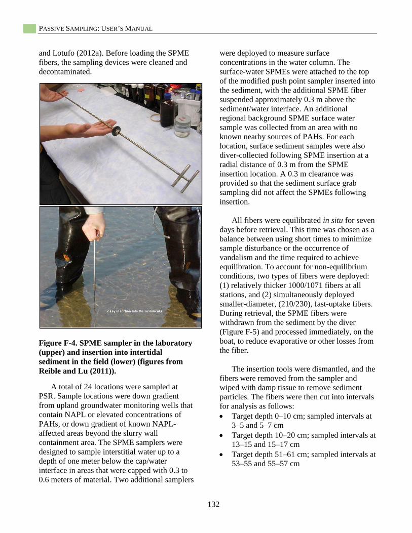
PASSIVE SAMPLING: USER’S MANUAL
132
and Lotufo (2012a). Before loading the SPME
fibers, the sampling devices were cleaned and
decontaminated.
Figure F-4. SPME sampler in the laboratory
(upper) and insertion into intertidal
sediment in the field (lower) (figures from
Reible and Lu (2011)).
A total of 24 locations were sampled at
PSR. Sample locations were down gradient
from upland groundwater monitoring wells that
contain NAPL or elevated concentrations of
PAHs, or down gradient of known NAPL-
affected areas beyond the slurry wall
containment area. The SPME samplers were
designed to sample interstitial water up to a
depth of one meter below the cap/water
interface in areas that were capped with 0.3 to
0.6 meters of material. Two additional samplers
were deployed to measure surface
concentrations in the water column. The
surface-water SPMEs were attached to the top
of the modified push point sampler inserted into
the sediment, with the additional SPME fiber
suspended approximately 0.3 m above the
sediment/water interface. An additional
regional background SPME surface water
sample was collected from an area with no
known nearby sources of PAHs. For each
location, surface sediment samples were also
diver-collected following SPME insertion at a
radial distance of 0.3 m from the SPME
insertion location. A 0.3 m clearance was
provided so that the sediment surface grab
sampling did not affect the SPMEs following
insertion.
All fibers were equilibrated in situ for seven
days before retrieval. This time was chosen as a
balance between using short times to minimize
sample disturbance or the occurrence of
vandalism and the time required to achieve
equilibration. To account for non-equilibrium
conditions, two types of fibers were deployed:
(1) relatively thicker 1000/1071 fibers at all
stations, and (2) simultaneously deployed
smaller-diameter, (210/230), fast-uptake fibers.
During retrieval, the SPME fibers were
withdrawn from the sediment by the diver
(Figure F-5) and processed immediately, on the
boat, to reduce evaporative or other losses from
the fiber.
The insertion tools were dismantled, and the
fibers were removed from the sampler and
wiped with damp tissue to remove sediment
particles. The fibers were then cut into intervals
for analysis as follows:
Target depth 0–10 cm; sampled intervals at
3–5 and 5–7 cm
Target depth 10–20 cm; sampled intervals at
13–15 and 15–17 cm
Target depth 51–61 cm; sampled intervals at
53–55 and 55–57 cm
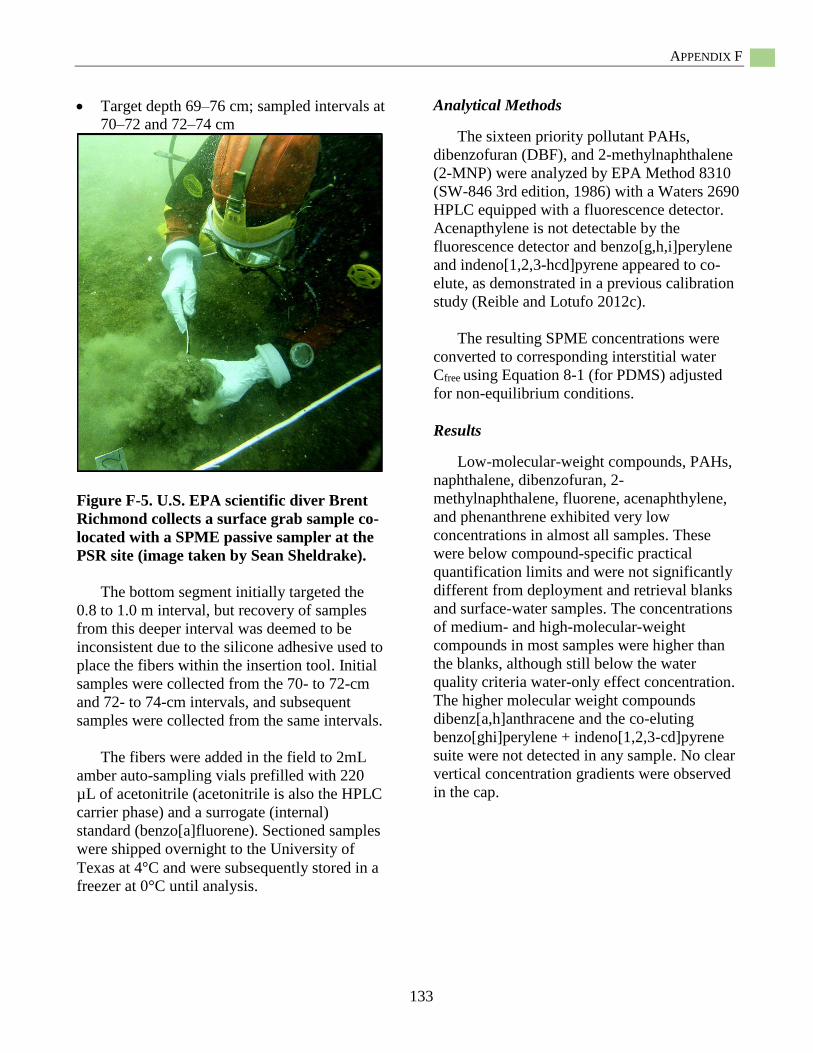
APPENDIX F
133
Target depth 69–76 cm; sampled intervals at
70–72 and 72–74 cm
Figure F-5. U.S. EPA scientific diver Brent
Richmond collects a surface grab sample co-
located with a SPME passive sampler at the
PSR site (image taken by Sean Sheldrake).
The bottom segment initially targeted the
0.8 to 1.0 m interval, but recovery of samples
from this deeper interval was deemed to be
inconsistent due to the silicone adhesive used to
place the fibers within the insertion tool. Initial
samples were collected from the 70- to 72-cm
and 72- to 74-cm intervals, and subsequent
samples were collected from the same intervals.
The fibers were added in the field to 2mL
amber auto-sampling vials prefilled with 220
µL of acetonitrile (acetonitrile is also the HPLC
carrier phase) and a surrogate (internal)
standard (benzo[a]fluorene). Sectioned samples
were shipped overnight to the University of
Texas at 4°C and were subsequently stored in a
freezer at 0°C until analysis.
Analytical Methods
The sixteen priority pollutant PAHs,
dibenzofuran (DBF), and 2-methylnaphthalene
(2-MNP) were analyzed by EPA Method 8310
(SW-846 3rd edition, 1986) with a Waters 2690
HPLC equipped with a fluorescence detector.
Acenapthylene is not detectable by the
fluorescence detector and benzo[g,h,i]perylene
and indeno[1,2,3-hcd]pyrene appeared to co-
elute, as demonstrated in a previous calibration
study (Reible and Lotufo 2012c).
The resulting SPME concentrations were
converted to corresponding interstitial water
Cfree using Equation 8-1 (for PDMS) adjusted
for non-equilibrium conditions.
Results
Low-molecular-weight compounds, PAHs,
naphthalene, dibenzofuran, 2-
methylnaphthalene, fluorene, acenaphthylene,
and phenanthrene exhibited very low
concentrations in almost all samples. These
were below compound-specific practical
quantification limits and were not significantly
different from deployment and retrieval blanks
and surface-water samples. The concentrations
of medium- and high-molecular-weight
compounds in most samples were higher than
the blanks, although still below the water
quality criteria water-only effect concentration.
The higher molecular weight compounds
dibenz[a,h]anthracene and the co-eluting
benzo[ghi]perylene + indeno[1,2,3-cd]pyrene
suite were not detected in any sample. No clear
vertical concentration gradients were observed
in the cap.

PASSIVE SAMPLING: USER’S MANUAL
134
Regulatory Use
EPA Region 10 concluded that, given that
the interstitial water concentrations of PAHs
were low and not clearly linked to site
contaminants or migration from upland sites, the
PSR sediment cap appeared to be functioning as
designed and is effectively containing site
contaminants.
Site Contact
Ravi Sanga, USEPA Region 10.
John Wakeman, USACE Seattle District
References
EPA Method 8310 (SW-846) 3rd edition, 1986.
Reible D, Lu X. 2011. Solid-Phase
Microextraction Field Deployment and Analysis
Pacific Sound Resources. Report prepared for
the USACE Seattle District and US EPA Region
10. University of Texas. February 14, 2011.
Reible D, Lotufo G. 2012a. Demonstration and
Evaluation of Solid Phase Microextraction for
the Assessment Of Bioavailability and
Contaminant Mobility. ESTCP Project ER-
200624. Available from:
http://www.serdp.org/content/download/15533/
176851/file/ER-200624-Guidance%20Doc.pdf.
Reible D, Lotufo G. 2012b. Demonstration and
Evaluation of Solid Phase Microextraction for
the Assessment of Bioavailability and
Contaminant Mobility. Final Report. ESTCP
Project ER-200624.
Reible D, Lotufo G. 2012c. Final Report.
Demonstration and Evaluation of Solid
Phase Microextraction for the Assessment
of Bioavailability and Contaminant Mobility.
ESTCP Project ER-200624. Available on the
web at:
http://www.serdp.org/content/download/5137/7
2968/file/ER-0624-Lab-Rep.pdf.
USEPA/USACE. 2010. Solid Phase
Microextraction Field Deployment and Analysis
Work Plan Pacific Sound Resources Superfund
Site. Seattle, WA. U.S. Environmental
Protection Agency Region 10, and the U.S.
Army Corps of Engineers Seattle District.
September 17, 2010. Available from:
http://www.epa.gov/region10/pdf/sites/psr/Field
_Deployment_Work_Plan.pdf.

APPENDIX F
135
Case Study 3: Wyckoff/Eagle Harbor
Superfund Site (East Harbor Operable
Unit), Bainbridge Island, Washington,
USA
Background
Target Contaminants:
Creosote-derived polycyclic aromatic
hydrocarbons (PAHs)
Passive Sampler:
Solid-phase microextraction (SPME) -
polydimethylsiloxane (PDMS)-coated fibers
Site Narrative
The Wyckoff/Eagle Harbor Superfund Site,
East Harbor Operable Unit (EHOU) is located
on Bainbridge Island, Washington. The site is a
former wood-treating facility that operated from
the early 1900s through 1988; pressure
treatment of utility poles with creosote and
bunker oil began in 1910. Relevant completed
remedial actions at the EHOU, to date, include:
Placement of a subtidal sediment cap,
completed in three phases between 1994 and
2002 (Figure F-6);
Upland source control, completed in
February 2001 by installation of a sheet-pile
wall around the perimeter of the former
process area;
Construction of an exposure barrier system
(EBS), completed in 2008, covering
approximately 300 linear meters of West
Beach and approximately 5.1 acres (2.06
hectares) from the southern edge of the
existing subtidal cap; and
Monitored natural recovery along the eastern
intertidal area
Monitoring of the marine portions of the
EHOU was conducted in 2011. The efficacy of
the subtidal cap is monitored principally by
collecting sediment grab and/or core samples,
chemical analyses, and comparison of the
resultant values to site human health remedial
action levels and the sediment management
standards (HDR et al, 2012). An additional
component of the 2011 monitoring was the
evaluation of whether PAHs were advecting in
interstitial water from the native contaminated
sediments up through the cap and into the
overlying water. Passive samplers co-located at
sediment sampling locations were used to
evaluate this potential pathway (Thomas et al.
2012).
Project Objectives
Evaluate whether near-surface cap interstitial
water concentrations exceed water quality
criteria effect concentrations for PAHs
Identify vertical profiles in PAH interstitial
water concentrations to ascertain whether
dissolved phase contaminants are migrating
through the subtidal cap
Compare depth discrete interstitial water
PAH concentrations determined by SPMEs
with measures made using integrated
interstitial water samples collected from bulk
sediment measurements.
Deployment and Retrieval of Passive Samplers
Details of the preparation, deployment,
retrieval and analyses reported here are from the
final report for the site (Thomas et al. 2012).
SPMEs were housed in a modified push point
sampling assembly developed by the University
of Texas. The samplers are piezometers that
have been modified to serve as a shielded sheath
for the SPME-PDMS coated glass fibers. Details
of the sampler and SPME fiber preparation
procedures are found in Reible and Lotufo
(2012).
Given the limited sampling period (7 days),
two methods were used to evaluate uptake and
estimate equilibrium dissolved concentrations of
PAHs. Two distinct SPME fibers were used:

PASSIVE SAMPLING: USER’S MANUAL
136
1000/1071-μm fiber (115 μL PDMS/m) and
1000/1060-μm fiber (97.1 μL PDMS/m). Second,
deuterated PAHs were impregnated into the
1000/1071-μm fiber as performance reference
compounds (PRCs). The four PRCs were
fluoranthene-d10, chrysene-d12, benzo[b]
fluoranthene-d12, and dibenz[a,h]anthracene-d14.
To adequately evaluate potential interstitial
water vertical profiles, cap thickness data were
used to select the appropriate sampler length. Of
specific import are stations G-8 where there was
only 0.61 m of capping material, and J9 where
there was little to no capping material over the
NAPL-contaminated sediments. Vertical
profiles of PAH concentrations were obtained
for depths of 30 to 90 cm from the
sediment/water interface based on the relative
cap thickness (Figure F-6). There were a total of
17 onsite deployments, and one offsite location
to serve as a reference station. Surface water-
column measurements were obtained using
fibers deployed approximately 30 cm above the
sediment/surface-water interface at three
locations—two onsite and one offsite—in a
nearby harbor located down gradient of the site
(Figure F-7).
The SPME samplers were deployed and
retrieved by EPA Region 10 divers (Figure F-8).
Six of the 90-cm samplers were loaded with
1000/1071-μm fibers spiked with PRCs to
assess the fraction of equilibrium attained
during the deployment. The deployed samplers
and the two field blanks were processed by
dismantling the samplers, removing the fibers
using a thin metal blade, and wiping with a
laboratory tissue dampened with deionized
water to remove any particulate matter. The
fibers were then sectioned into adjacent 2-cm
fiber segments, placed in prefilled vial inserts
containing acetonitrile, and shipped on ice back
to the University of Texas in Austin.
Analytical Method
The PDMS solvent extracts were transferred
from the original vial insert to a new vial insert
to avoid interference from the fiber during
analysis. The PDMS solvent extracts were
analyzed using high-performance liquid
chromatography (HPLC) according to EPA
Method 8310. Ultraviolet (UV) and
fluorescence (FLD) detectors were used to
quantify the EPA 16 priority PAHs.
Chromatographic separation was conducted
using a 1.0 mL/min isocratic flow composed of
3:7 (v:v) water:acetonitrile.
Limitations to this analytical method
include: acenaphthylene cannot be analyzed by
fluorescence detector, and the method detection
limit (MDL) is 20 μg/L with UV, and
benzo[g,h,i]perylene and indeno[1,2,3-
cd]pyrene coelute and must be reported as a
single combined concentration.
The interstitial water Cfree was determined
based on the reported HPLC-measured
concentration, the volume of solvent used to
extract the fiber, the length of fiber sample,
specific volume of the fiber, and PAH KPDMS.
The KPDMS were determined by Reible (2010).
Equilibrium correction factors were determined
based on the PRC loss over the seven day
sampling period, and were applied to all
sampling locations to determine the absolute
interstitial water Cfree at those locations.
The resultant interstitial water
concentrations were compared to EPA’s
Ambient Water Quality Criteria (AWQC) for
PAHs, and to the measures of PAHs made in the
overlying surface water. To compare the
measured interstitial water concentrations to
estimated interstitial water concentrations, the
sampled SPME intervals were matched to the
bulk sediment PAH and total organic carbon
measures from a 2011 report (HDR 2012).

APPENDIX F
137
Notes:1. Horizontal control based on WA coordinate system
north zone, NAD 8391
SPME Deployment Locations
1994 Phase I Cap Boundary2000 Phase II Cap Boundary
2001 Phase III Cap BoundaryExposure Barrier System
Figure F-6. Cap Boundary areas and SPME sampling locations. SPME sampling locations were placed on transects from the shore
and were co-located with bulk sediment sampling locations. Two SPMEs were deployed in surface water ~ 0.3 m above the sediment
surface between G-8 and H-9.5 (designated sample SW-1) and H-10 and H-10.5 (SW-2). (Base figure from HDR et al. (2012).
Sampling location figure from Thomas et al. (2012)).
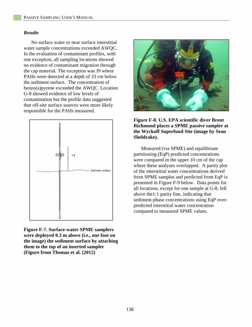
PASSIVE SAMPLING: USER’S MANUAL
138
Results
No surface water or near surface interstitial
water sample concentrations exceeded AWQC.
In the evaluation of contaminant profiles, with
one exception, all sampling locations showed
no evidence of contaminant migration through
the cap material. The exception was J9 where
PAHs were detected at a depth of 33 cm below
the sediment surface. The concentration of
benzo(a)pyrene exceeded the AWQC. Location
G-8 showed evidence of low levels of
contamination but the profile data suggested
that off-site surface sources were more likely
responsible for the PAHs measured.
Figure F-7. Surface-water SPME samplers
were deployed 0.3 m above (i.e., one foot on
the image) the sediment surface by attaching
them to the top of an inserted sampler
(Figure from Thomas et al. (2012)
Figure F-8. U.S. EPA scientific diver Brent
Richmond places a SPME passive sampler at
the Wyckoff Superfund Site (image by Sean
Sheldrake).
Measured (via SPME) and equilibrium
partitioning (EqP) predicted concentrations
were compared in the upper 10 cm of the cap
where these analyses overlapped. A parity plot
of the interstitial water concentrations derived
from SPME samples and predicted from EqP is
presented in Figure F-9 below. Data points for
all locations, except for one sample at G-8, fell
above the1:1 parity line, indicating that
sediment-phase concentrations using EqP over-
predicted interstitial water concentration
compared to measured SPME values.

APPENDIX F
139
0.000001
0.00001
0.0001
0.001
0.01
0.1
1
10
100
0.000001 0.0001 0.01 1 100
Pore
wat
er C
once
ntr
atio
n d
eriv
ed f
rom
Gra
b
Sam
ple
(ug/L
)
Porewater Concentration measured using SPME (ug/L)
I-8
I-9
I-10
I-10 Duplicate
G-8
J-9a
J-9b
J-9b Duplicate
J-9c
H-9
G-9
F-9
1:1 Line
Figure F-9. Parity plot of PAH concentrations between SPME interstitial water concentrations
and interstitial water concentrations inferred by equilibrium partitioning from grab sample
measurements (HDR et al. (2012)).
Regulatory Use
Efficacy of the subtidal cap was further
demonstrated by the SPME data. Overall, the
concentrations measured in surface samples did
not exceed the AWQC, with the exception of
location J-9. The OMMP report had shown
there was little to no capping material over the
contaminated native sediments at J-9 (HDR et
al. 2012).
Costs
Analytical costs were $425/sample. This is
based on a reported total cost of $62,000 for
146 samples (Thomas et al. 2012). This cost
represents only preparation and analysis time;
the cost of the field deployment and retrieval
by the EPA dive team was not available.
Site Contact
Mandy Michelson, USACE Seattle District
Howard Orlean, EPA Region 10, Washington.
PASSIVE SAMPLING: USER’S MANUAL
140
References
HDR. 2012. 2011 year 17 monitoring report
East Harbor Operable Unit Wyckoff/Eagle
Harbor Superfund Site. Final dated September
7, 2012. Prepared for the U.S. Environmental
Protection Agency, Region 10 Seattle WA, and
the U.S. Army Corps of Engineers Seattle
District. Prepared by HDR Engineering Inc,
Olympia WA; SEE LLC, Seattle, WA; Ken
Taylor and Associates, Seattle, WA.
Reible, DD. 2010. SPME/PDMS calibration
study. Final report to Northwest Division
Seattle District US Army Corps of Engineers,
April 2010.
Reible D, Lotufo G. 2012. Demonstration and
Evaluation of Solid Phase Microextraction for
the Assessment of Bioavailability and
Contaminant Mobility. ESTCP Project ER-
200624. Available from:
http://www.serdp.org/content/download/15533/
176851/file/ER-200624-Guidance%20Doc.pdf
Thomas C, Lu X, Reible D. 2012. Draft
Wyckoff cap performance evaluation, solid‐phase microextraction field deployment and
analysis, Wyckoff/Eagle Harbor. University of
Texas, Austin, TX.
APPENDIX F
141
Case Study 4: United Heckathorn
Superfund Site (Lauritzen Channel,
Inner Richmond Harbor), California.
Background
Target Contaminants:
DDT and degradation products
(i.e., DDE and DDD), dieldrin
Passive Sampler:
Low-density polyethylene (LDPE)
Site Narrative
The United Heckathorn Superfund site is
located in the Richmond Inner Harbor of San
Francisco Bay. The site includes an upland area
(~5 acres) and a marine portion (~25 acres) that
comprises two channels, the Lauritzen Channel
and the Parr Channel. Between 1947 and 1966,
onshore activities at this site included
formulating, packaging, and shipping of DDT,
dieldrin, and other pesticides. In 1996–1997,
remedial action involved excavation and
addition of a cap on the upland area, and
dredging of both channels.
Post-remediation monitoring found that the
remedial actions were not sufficient in the area
of the Laurizten Channel. In a five-year review
published in 2011, EPA concluded that the
levels of DDT in the sediments of the Lauritzen
Channel were still hazardous for human and
ecosystem health (US EPA, 2011). Further
sampling efforts (2011–2014) at the site,
including polyethylene passive samplers in the
sediments and water column, were used to
determine the source of the post-remediation
DDT levels in the Lauritzen Channel
sediments, and to inform clean-up decision
making.This site is another example where U.S.
EPA scientific divers from the Environmental
Response Team deployed and recovered the
passive samplers insuring proper sampler
placement, and data quality and integrity.
Objectives
Delineate the problematic sediments in the
Laurizten Channel with the help of in situ
LDPE samplers deployed at various locations
in the channel
Determine the direction and estimate the
magnitude of the sediment-to-water flux based
on the passive sampler deployed across the
sediment/water interface
Evaluate with a mass balance model for surface
water in the channel, whether the calculated
sediment-to-water fluxes can account for the
observed concentrations of DDX (DDT and
degradates DDE and DDD) in that water
column
Field Deployments
Polyethylene (PE) strips loaded with
performance reference compounds (PRCs)
were mounted in rectangular aluminum frames
(Figure F-10). The samplers were deployed for
31 days at the sediment/water interface, at
various sites across the channel (Figure F-11),
at ten stations in 2013 [see Gschwend 2014]—
and at eight stations in 2012 [see Gschwend
and Burgess 2012]). With the help of divers,
the samplers were pushed into the sediment
bed, such that a portion of the LDPE strip
remained above the sediment bed to sample the
overlying bottom water. In addition, LDPE
strips were deployed higher in the water
column, to infer truly dissolved DDX
concentrations. After retrieval, the LDPE strips
were cleaned, sectioned into 5-cm pieces, and
placed in VOA vials for extraction and
analysis.
Analytical Procedures
The sectioned LDPE strips were spiked
with surrogate standards (also known as
internal standards) and extracted three times
with dichloromethane. The extracts were
concentrated, exchanged to hexane, and spiked
with injection compounds. Finally, the extracts

PASSIVE SAMPLING: USER’S MANUAL
142
were analyzed using gas chromatography-mass
spectrometry (GC-MS) with cold on column
injections. Field blank samplers (i.e., LDPE
strips mounted in frames and taken to the field
but not deployed) were also analyzed to
determine the initial PRC concentrations
(procedures described in more detail in
Gschwend 2014).
Figure F-10. Assembly of samplers
prior to deployment (top), and a sampler
after retrieval (bottom), showing the
sediment/water interface right above the
white tape mark. The total length of the
LDPE window was ~50 cm.
To determine freely dissolved
concentrations (Cfree), the measured
concentrations of target analytes in the LDPE
samplers were first corrected by the fractional
equilibration calculated from the PRC loss.
These LDPE concentrations were then adjusted
by the low-density polyethylene-water partition
coefficient of each analyte to ascertain the
corresponding interstitial water or surface-
water Cfree (Equation 8-2).
Results
Distribution of contaminants across the
channel showed a gradient in concentration,
with interstitial water concentrations exceeding
1000 ng/L of 4,4-DDD in the northern-most
parts of the channel and decreasing to ~10 ng/L
of 4,4-DDD in the southern-most sampling
sites. The interstitial water concentrations were
typically larger than the bottom-water
concentrations, implying a flux out of the
sediment. The differences between the
interstitial water concentrations measured in the
top sediment layer (5 cm) and the bottom water
varied across the sampling sites, being larger in
the northern than in the southern portion of the
channel (Figure F-12).
Assuming that the sediment bed is the only
source of contamination, and that the only
removal of contaminants from the channel is
due to the tidal action, a simple mass balance
model was used to estimate the steady-state
water-column concentration. Given the strong
declining trend in interstitial water
concentrations from north to south, the channel
was split into four sections (or boxes), and an
average sediment-to-water flux of DDT, DDE,
and DDD was calculated for each box.
Assuming that the tidal flushing displaced
water between consecutive boxes, the steady-
state concentrations of the DDX in the water
column were calculated and compared to the
measured concentrations from water column
samplers.

APPENDIX F
143
Figure F-11. Map of locations in Lauritzen Channel for deployment of
samplers at the sediment/water interface in 2012 (pink) and 2013 (green).
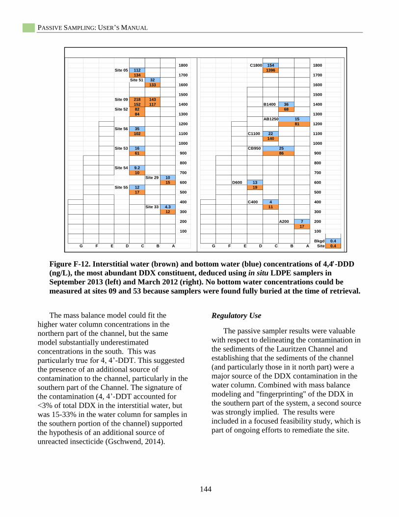
PASSIVE SAMPLING: USER’S MANUAL
144
1800
Site 05 112
134 1700
Site 51 32
133 1600
1500
Site 09 218 143
152 117 1400
Site 52 82
84 1300
1200
Site 56 35
102 1100
1000
Site 53 16
61 900
800
Site 54 9.2
10 700
Site 29 10
15 600
Site 55 12
17 500
400
Site 33 4.3
12 300
200
100
G F E D C B A
C1800 154 1800
1396
1700
1600
1500
B1400 36 1400
68
1300
AB1250 15
81 1200
C1100 22 1100
140
1000
CB950 25
86 900
800
700
D600 13 600
19
500
C400 4 400
11
300
A200 7 200
17
100
Bkgd 0.4
G F E D C B A Site 0.4
Figure X. Comparison of porewater (brown) and bottom water (blue) concentrations of 4,4'-DDD (ng/L) deduced using PE passive samplers in the field in Sept 2013 (left) and March 2012 (right).
Figure F-12. Interstitial water (brown) and bottom water (blue) concentrations of 4,4-DDD
(ng/L), the most abundant DDX constituent, deduced using in situ LDPE samplers in
September 2013 (left) and March 2012 (right). No bottom water concentrations could be
measured at sites 09 and 53 because samplers were found fully buried at the time of retrieval.
The mass balance model could fit the
higher water column concentrations in the
northern part of the channel, but the same
model substantially underestimated
concentrations in the south. This was
particularly true for 4, 4’-DDT. This suggested
the presence of an additional source of
contamination to the channel, particularly in the
southern part of the Channel. The signature of
the contamination (4, 4’-DDT accounted for
<3% of total DDX in the interstitial water, but
was 15-33% in the water column for samples in
the southern portion of the channel) supported
the hypothesis of an additional source of
unreacted insecticide (Gschwend, 2014).
Regulatory Use
The passive sampler results were valuable
with respect to delineating the contamination in
the sediments of the Lauritzen Channel and
establishing that the sediments of the channel
(and particularly those in it north part) were a
major source of the DDX contamination in the
water column. Combined with mass balance
modeling and "fingerprinting" of the DDX in
the southern part of the system, a second source
was strongly implied. The results were
included in a focused feasibility study, which is
part of ongoing efforts to remediate the site.

APPENDIX F
145
Site Contact
EPA Site Manager: Rachelle Thompson
415-972-3962
US EPA Region 9
Mail Code SFD
75 Hawthorne Street
San Francisco, CA 94105
References
USEPA (U.S. Environmental Protection
Agency). 2011. Third five-year review report
for United Heckathorn Superfund site,
Richmond, Contra Costa County, California.
September.
Gschwend, P.M., and Burgess, R.M. 2012.
Application of passive samplers to assess
dissolved DDTs in the Lauritzen Channel at the
United Heckathorn site in Richmond Harbor,
San Francisco Bay. Prepared for U.S.
Environmental Protection Agency Region 9.
November.
Gschwend, P. M. 2014. Application of
polyethylene (PE) passive samplers to assess
DDTs in the Lauritzen Channel at the United
Heckathorn site in Richmond Harbor, San
Francisco Bay. Included in United Heckathorn
Superfund Site, Richmond, California DDT
Fate and Transport Study, available at
http://yosemite.epa.gov/r9/sfund/r9sfdocw.nsf/
3dc283e6c5d6056f88257426007417a2/d9263f
b3f9c7358e88257d18005d365d/$FILE/Final_H
eckathorn_DDT_FateAndTransport.pdf
PASSIVE SAMPLING: USER’S MANUAL
146
Case Study 5: Site Assessment of
Sediment Toxicity, San Diego Bay,
California, USA
Background
Target Contaminants: Metals
Passive Sampler: Diffusive gradients in thin
films (DGTs)
Site Narrative
The Sediment Ecotoxicity Assessment
(SEA) Ring was developed as an integrated
exposure and effects assessment system.
Validation experiments were conducted in 2010
and 2011 in San Diego Bay, California as part
of extensive proof-of-concept studies. During
these studies, DGTs were deployed within SEA
Ring exposure chambers (Figure F-13) to
provide further assessment of labile fractions of
metals in sediments (Burton et al. 2012).
Several pier areas in San Diego Bay have
been listed as potentially at risk for aquatic life
impacts. Four sediment locations were
evaluated in San Diego Bay during the studies.
Three locations used had historical data
indicating sediment contamination and possibly
contaminated upwelling groundwaters. A
fourth location was the reference site. Test
organisms deployed on the SEA Ring included
the amphipod, Leptocheirus plumulosus, the
polychaete, Neanthes arenaceodentata, the
mysid, Americamysis bahia, and the clam,
Mercenaria mercenaria. The SEA Rings
contained up to 14 exposure chambers. Also,
placing multiple species in a single chamber
allowed for a minimum of four replicate
chambers for each toxicity and bioaccumula-
tion endpoint. Surface water and upwelling
groundwaters were sampled and monitored
with in situ water quality sensors for
temperature, depth, dissolved oxygen, pH,
salinity, conductivity, and oxidation-reduction
potential. In situ interstitial water Cfree was
measured using the solid-phase microextraction
devices (SPMEs), DGTs, and Trident probe
samplers for volatile organic compounds
(VOCs), polycyclic aromatic hydrocarbons
(PAHs), metals, and dissolved organic carbon.
Project Objectives
Improve on the efficiency and accuracy of
site assessments of ecosystem risk and
recovery (following remedial actions) by
simultaneously measuring exposures of
contaminants and effects in multiple species
of benthic and pelagic organisms (overall).
Provide information from the DGTs on
labile metal exposures and their vertical and
horizontal gradients at the test sites.
Deployment and Retrieval of Passive Samplers
The DGTs were purchased from DGT
Research, Ltd., and consisted of a diffusive gel
protected by a plastic housing. DGTs were
deployed within the SEA Ring surficial
sediment exposure chambers using a custom
holder at each of the four study locations. The
DGTs were positioned vertically, so that the
majority of the passive sampler would be
buried in the sediment. About one-third of the
device was exposed to the water column, and
the remaining two-thirds contacted the
sediment. The portion of the device exposed to
the water column was to provide shallow
interstitial water and overlying water
measurements (Burton et al. 2012).
Analytical Method
After 48 hours, the DGTs were removed,
rinsed in deionized water, sectioned into 1-cm
vertical slices, acidified, and analyzed for Cu,
Zn, Ni, Pb, and Cd using EPA Method 200.8.
Metal concentrations in elutriate were
converted to DGT concentrations (CDGT) using
temperature-specific diffusion coefficients (see
Section 8).
APPENDIX F
147
Results
DGT deployments in contaminated
sediments revealed gradients across the sites,
with elevated levels of Zn, followed by Ni and
Pb in the top 5 cm of sediments. Cu was
recovered only in the deeper sediments.
Toxicity and tissue residue results showed
some relationships with PAHs collected in the
SPMEs, but not with the labile fractions
recovered in the DGTs .The metal
concentrations observed in the interstitial
waters were well below published toxicity
thresholds. The infaunal bivalve tissue
concentrations (21-day exposures) of metals
suggested they were not causing toxicity.
Regulatory Use
DGTs can provide an additional line of
evidence when evaluating sites that have
multiple chemical contaminants and are being
considered for remediation.
Site Contact
Gunther Rosen
SPARWAR Systems Center Pacific
53475 Strohe Rd., Bldg. 1111
San Diego, CA 92152
Tel 619-553-0886

PASSIVE SAMPLING: USER’S MANUAL
148
Figure F-13. Side view of the SEA Ring exposure chambers, including options for overlying
water (WC), sediment/water interface (SWI), or surficial sediment (SED) exposures. Passive
samplers are also integrated into chambers, as shown for DGT (Figure from Burton et al.
(2012)).
Reference
Burton Jr. GA, Rosen G, Chadwick DB,
Greenberg MS, Taulbee WK, Lotufo GR, Reible
DD. 2012. A Sediment Ecotoxicity Assessment
Platform for in situ Measures of Chemistry,
Bioaccumulation and Toxicity. Part 1: System
Description and Proof of Concept. U.S. Navy
Research. Paper 29.

APPENDIX F
149
Case Study 6: Ex situ Passive
Sampling Measurement of Site-
Specific Partitioning of PAHs and
PCBs in Sediments
Background
Target Contaminants:
Polycyclic aromatic hydrocarbons (PAHs)
and polychlorinated biphenyls (PCBs)
Passive Sampler:
Low density polyethylene – ex situ
laboratory exposure
Site Narrative
The South Wilmington Wetlands adjoining
the Christiana River in Delaware has
experienced historical waste disposal and
impacts from past industrial and commercial
activities. A 22 acre portion of the wetlands is
under active investigation for potential
ecological and human health concerns and
options for a final remedy. Key contaminants
of concern include PAHs, PCBs, a suite of
metals, and pesticides. Initial site
investigations indicated that several chemicals
of concern present in the soils and sediments
can potentially pose ecological risk to aquatic
and terrestrial animals that can come in contact
with the media. To advance the restoration
process of the wetlands, it was determined that
‘preliminary remediation goals (PRGs)’ need to
be set for the chemicals of concern allowing for
conceptualization of the extent of the
contamination problem and initiating
evaluation of the potential remedial options for
the site. Initial development of the site
sediment guidelines were based on equilibrium
partitioning sediment benchmarks (USEPA
2003 for PAHs and pesticides) which use
organic carbon normalized partition constants
(KOC) to convert water-only final chronic
values (FCVs) to sediment phase Equilibrium
Partitioning Sediment Benchmarks (ESB). A
very critical parameter in the calculation of the
ESBs is the KOC, which is often estimated for
the site based on literature values. While the
traditional practice uses default values for KOC,
recent work indicates that site specific values
can often be several orders of magnitude
different from default values (Hawthorne et al.
2006). U.S. EPA guidance on sediment risk
assessment also cautions against the use of
default values and provides suggestions for
using site specific measurement of partition
constants (U.S. EPA 2012a) to refine the
assessment of risk. One of the reasons for the
common use of default partitioning values in
the past has been the difficulty and expense
associated with accurate measurement of low
concentrations of dissolved phase HOCs in
sediments. However, recent advances in the
use of passive sampling to measure equilibrium
partitioning has made it possible to
conveniently measure site-specific partitioning
of a wide range of HOCs in sediments (U.S.
EPA 2012b; Ghosh et al. 2014).
Project Objectives
The primary objective of this study was to
determine the site-specific equilibrium
partitioning constants for PAHs and PCBs in
sediments from the South Wilmington
Wetlands and use those values to refine the
development of PRGs for the site. It was
anticipated that a site-specific assessment of
partitioning would allow more accurate
assessment of the risk posed by the chemicals
of concern and the development of a more
targeted management plan to reduce remaining
risk.
Laboratory Deployment
To allow accurate calculation of KOC values
for the strongly hydrophobic compounds,
passive sampling technique was used to
measure the equilibrium interstitial water
concentration of PAHs and PCBs in the
sediment. Briefly, the method involved
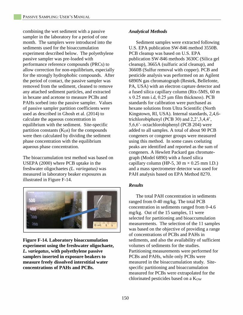
PASSIVE SAMPLING: USER’S MANUAL
150
combining the wet sediment with a passive
sampler in the laboratory for a period of one
month. The samplers were introduced into the
sediments used for the bioaccumulation
experiment described below. The polyethylene
passive sampler was pre-loaded with
performance reference compounds (PRCs) to
allow correction for non-equilibrium, especially
for the strongly hydrophobic compounds. After
the period of contact, the passive sampler was
removed from the sediment, cleaned to remove
any attached sediment particles, and extracted
in hexane and acetone to measure PCBs and
PAHs sorbed into the passive sampler. Values
of passive sampler partition coefficients were
used as described in Ghosh et al. (2014) to
calculate the aqueous concentration in
equilibrium with the sediment. Site-specific
partition constants (KDs) for the compounds
were then calculated by dividing the sediment
phase concentration with the equilibrium
aqueous phase concentration.
The bioaccumulation test method was based on
USEPA (2000) where PCB uptake in the
freshwater oligochaetes (L. variegatus) was
measured in laboratory beaker exposures as
illustrated in Figure F-14.
Figure F-14. Laboratory bioaccumulation
experiment using the freshwater oligochaete,
L. variegatus, with polyethylene passive
samplers inserted in exposure beakers to
measure freely dissolved interstitial water
concentrations of PAHs and PCBs.
Analytical Methods
Sediment samples were extracted following
U.S. EPA publication SW-846 method 3550B.
PCB cleanup was based on U.S. EPA
publication SW-846 methods 3630C (Silica gel
cleanup), 3665A (sulfuric acid cleanup), and
3660B (Sulfur removal with copper). PCB and
pesticide analysis was performed on an Agilent
6890N gas chromatograph (Restek, Bellefonte,
PA, USA) with an electron capture detector and
a fused silica capillary column (Rtx-5MS, 60 m
x 0.25 mm i.d, 0.25 μm film thickness). PCB
standards for calibration were purchased as
hexane solutions from Ultra Scientific (North
Kingstown, RI, USA). Internal standards, 2,4,6-
trichlorobiphenyl (PCB 30) and 2,2’,3,4,4’,
5,6,6’- octachlorobiphenyl (PCB 204) were
added to all samples. A total of about 90 PCB
congeners or congener groups were measured
using this method. In some cases coeluting
peaks are identified and reported as the sum of
congeners. A Hewlett Packard gas chromate-
graph (Model 6890) with a fused silica
capillary column (HP-5, 30 m × 0.25 mm I.D.)
and a mass spectrometer detector was used for
PAH analysis based on EPA Method 8270.
Results
The total PAH concentration in sediments
ranged from 0-40 mg/kg. The total PCB
concentration in sediments ranged from 0-4.6
mg/kg. Out of the 15 samples, 11 were
selected for partitioning and bioaccumulation
measurements. The selection of the 11 samples
was based on the objective of providing a range
of concentrations of PCBs and PAHs in
sediments, and also the availability of sufficient
volumes of sediments for the studies.
Partitioning measurements were performed for
PCBs and PAHs, while only PCBs were
measured in the bioaccumulation study. Site-
specific partitioning and bioaccumulation
measured for PCBs were extrapolated for the
chlorinated pesticides based on a KOW
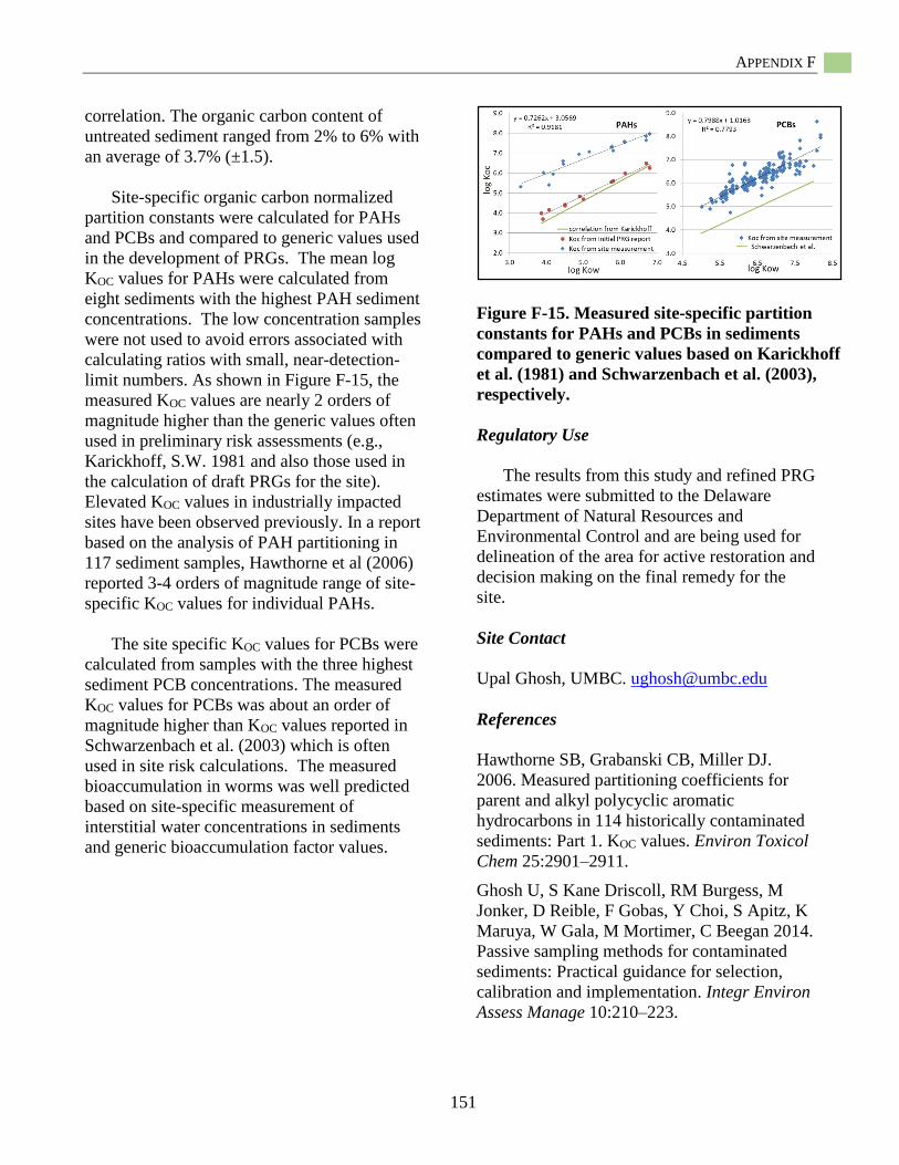
APPENDIX F
151
correlation. The organic carbon content of
untreated sediment ranged from 2% to 6% with
an average of 3.7% (±1.5).
Site-specific organic carbon normalized
partition constants were calculated for PAHs
and PCBs and compared to generic values used
in the development of PRGs. The mean log
KOC values for PAHs were calculated from
eight sediments with the highest PAH sediment
concentrations. The low concentration samples
were not used to avoid errors associated with
calculating ratios with small, near-detection-
limit numbers. As shown in Figure F-15, the
measured KOC values are nearly 2 orders of
magnitude higher than the generic values often
used in preliminary risk assessments (e.g.,
Karickhoff, S.W. 1981 and also those used in
the calculation of draft PRGs for the site).
Elevated KOC values in industrially impacted
sites have been observed previously. In a report
based on the analysis of PAH partitioning in
117 sediment samples, Hawthorne et al (2006)
reported 3-4 orders of magnitude range of site-
specific KOC values for individual PAHs.
The site specific KOC values for PCBs were
calculated from samples with the three highest
sediment PCB concentrations. The measured
KOC values for PCBs was about an order of
magnitude higher than KOC values reported in
Schwarzenbach et al. (2003) which is often
used in site risk calculations. The measured
bioaccumulation in worms was well predicted
based on site-specific measurement of
interstitial water concentrations in sediments
and generic bioaccumulation factor values.
Figure F-15. Measured site-specific partition
constants for PAHs and PCBs in sediments
compared to generic values based on Karickhoff
et al. (1981) and Schwarzenbach et al. (2003),
respectively.
Regulatory Use
The results from this study and refined PRG
estimates were submitted to the Delaware
Department of Natural Resources and
Environmental Control and are being used for
delineation of the area for active restoration and
decision making on the final remedy for the
site.
Site Contact
Upal Ghosh, UMBC. [email protected]
References
Hawthorne SB, Grabanski CB, Miller DJ.
2006. Measured partitioning coefficients for
parent and alkyl polycyclic aromatic
hydrocarbons in 114 historically contaminated
sediments: Part 1. KOC values. Environ Toxicol
Chem 25:2901–2911.
Ghosh U, S Kane Driscoll, RM Burgess, M
Jonker, D Reible, F Gobas, Y Choi, S Apitz, K
Maruya, W Gala, M Mortimer, C Beegan 2014.
Passive sampling methods for contaminated
sediments: Practical guidance for selection,
calibration and implementation. Integr Environ
Assess Manage 10:210–223.
PASSIVE SAMPLING: USER’S MANUAL
152
Karickhoff SW. 1981. Semi-empirical
estimation of sorption of hydrophobic
pollutants on natural sediments and soils.
Chemosphere 10(8):833–846.
Lohmann R, Macfarlane JK, Gschwend PM.
2005. Importance of black carbon to sorption of
native PAHs, PCBs and PCDDs in Boston and
New York harbor sediment. Environ. Sci.
Technol. 39:141–148.
Schwarzenbach RP, Gschwend PM, Imboden,
DM. 2003. Environmental Organic Chemistry.
John Wiley and Sons. Princeton, NJ.
U.S. EPA 2012a. Equilibrium Partitioning
Sediment Benchmarks (ESBs) for the
Protection of Benthic Organisms: Procedures
for the Determination of the Freely Dissolved
Interstitial Water Concentrations of Nonionic
Organics. EPA/600/R-02/012. Office of
Research and Development. Washington, DC.
U.S. EPA 2012b. Guidelines for Using Passive
Samplers to Monitor Organic Contaminants at
Superfund Sediment Sites. OSWER Directive
9200.1–110FS. Office of Research and
Development. Washington, DC.
U.S. EPA. 2003. Procedures for the derivation
of equilibrium partitioning sediment
benchmarks (ESBs) for the protection of
benthic organisms: PAH mixtures. EPA-600-R-
02-013. Office of Research and Development,
Washington, DC.
U.S. EPA. 2000. Methods for Measuring the
Toxicity and Bioaccumulation of Sediment
Associated Contaminants with Freshwater
Invertebrates. EPA/600/R-99/064, Office of
Research and Development, Washington, DC.
Werner D, Hale SE, Seokjoon K, Ghosh U,
Luthy RG. 2011. Polychlorinated biphenyl
sorption and availability in field-contaminated
sediments. Environ Sci Technol 44:2809–2815.
APPENDIX G
153
Appendix G: Example Quality
Assurance Project Plan (QAPP) Two examples of quality assurance project
plans (QAPPs) are provided in Appendix G.
The first example is a interstitial water
Sampling and Analysis Plan (SAP) that was
prepared for the U.S. EPA’s Region 10 as part
of the River Mile 11 East (RM11E)
Supplemental Remedial Investigation and
Feasibility Study. The plan was prepared on
behalf of the RM11E Group by Science and
Engineering for the Environment, LLC (SEE),
Dalton, Olmstead and Fuglevand, Inc. (DOF),
and GSI Water Solutions, Inc. (GSI). The SAP
was prepared in response to U.S. EPA’s
communications to the RM11E Group
requiring the performance of a interstitial water
investigation as part of the data gathering effort
under the project work plan. PCBs were the
focus of the study.
The second example was prepared for the
U.S. EPA’s Region 9 Superfund program for
water column-based passive sampling research
investigating the flux of dissolved chlorinated
pesticides (i.e., DDTs) and PCBs from
contaminated sediments into the water column.
Note that standard operating procedures (SOPs)
appended to the plan were prepared by the
Southern California Coastal Water Research
Project (SCCWRP), Costa Mesa, California,
USA.
These documents can be found at these sites:
https://www.epa.gov/superfund/superfund-
contaminated-sediments-guidance-documents-
fact-sheets-and-policies.
and
https://www.serdp-estcp.org/Featured-
Initiatives/Cleanup-initiatives/Bioavailability
Further guidance on the preparation of a
QAPP is available from the Intergovernmental
Data Quality Task Force document, Uniform
Federal Policy for Quality Assurance Project
Plan. Evaluating, Assessing, and Documenting
Environmental Data Collection and Use
Programs. Part 1: UFP-QAPP Manual Final
Version 1. March 2005, EPA: EPA-505-B-04-
900A DoD: DTIC ADA 42778. The document
can also be downloaded from:
https://www.epa.gov/sites/production/files/doc
uments/ufp_qapp_v1_0305.pdf


