Page 1
Classical Mechanics Page No. 1
LAGRANGE'S FORMULATION
Unit 1:
In mechanics we study particle in motion under the action of a force.
Equation of motion describes how particle moves under the action of a force.
However, every motion of a particle is not free motion, but rather it is restricted by
putting some conditions on the motion of a particle or system of particles. Hence the
basic concepts like equations of motion, constraints and type of constraints on the
motion of a particle, generalized coordinates, conservative force, conservation
theorems, D’Alembert’s principle, etc. on which the edifice of mechanics is built are
illustrated in this unit.
• Introduction :
Mechanics is a branch of applied mathematics deals with the motion
of a particle or a system of particle with the forces Suppose a bullet is fired from a
fixed point with initial velocity u, not exactly vertically upward but making an angle
α with the horizontal. Then
what instruments do
mathematicians need to find the
position of the bullet at some
instant latter, its velocity at that
instant, the distance covered by
the bullet at that instant and also
the path followed by the bullet at
the end of its journey?
mg
x.
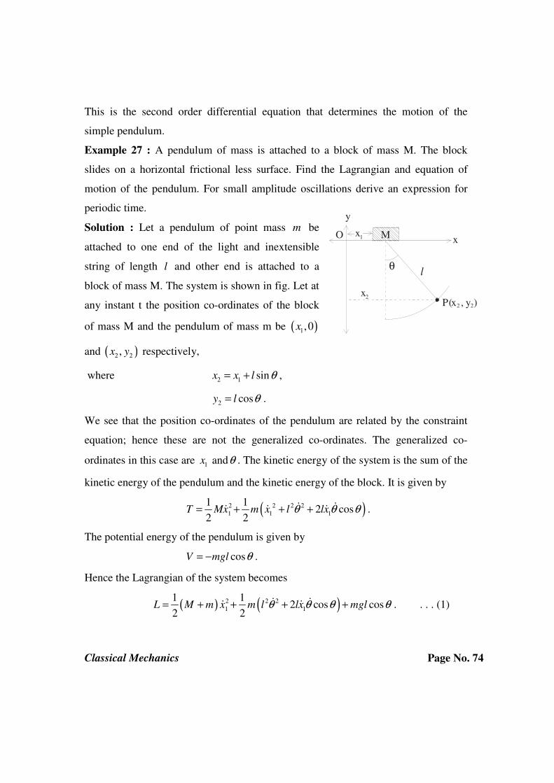
= u cosα
y.
= u sin α - gty.
= u sin α
x.
= u cosαOx
y
u
α
CHAPTER - I
Page 2
Classical Mechanics Page No. 2
Well, to answer such questions, mathematicians do not need any meter stick
to measure the distance covered by the bullet at the instant, they don't need any
speedometer to find its speed at any instant t, nor they need any clock to see the time
required to cover the definite distance. In fact, they need not have to do any such
experiment. What they need to describe the motion of the bullet are simply the co-
ordinates. Hence the single most important notion in mechanics is the concept of co-
ordinates. But the co-ordinates however, just play a role of markers or codes and will
no way influence or affect the motion of the bullet. These are just mathematical tools
in the hands of a mathematician. Thus the instruments in the hands of a
mathematician are the co-ordinates. With the help of these co-ordinates, the motion
of a particle or system of particle can completely be described.
For instance, to discuss the motion of the bullet, take P(x, y) be any point on
the path of the bullet. The only force acting on the bullet is the gravitational force in
the downward direction. Resolving this force horizontally and vertically, we write
from Newton's second law of motion the equations of motion as
0,
.
x
y g
=
= −
��
�� . . . (1)
Integrating the above two equations and using the initial conditions we
readily obtain
cos ,
sin ,
x u
y u gt
α
α
=
= −
�
� . . . (2)
where u is the initial velocity of the bullet when t = 0. Integrating equations (2) once
again and using the initial conditions we obtain
cos ,x u tα= ⋅ . . . (3)
21sin
2y u t gtα= − . . . . (4)
Page 3
Classical Mechanics Page No. 3
Equations (2) determine the velocity of the bullet at any time t, while equations (3)
and (4) determine the position of the bullet at that instant. Further, eliminating t from
equations (3) and (4), we get
2
2 2
1tan
2 cos
gxy x
uα
α= − . . . . (5)
This equation gives the path of the bullet and the path is a parabola.
However, the co-ordinates used to describe the motion of a particle or system
of particles must be linearly independent. If not then the number of equations
describing the motion of the system will be less than the number of variables and in
this case the solution can not be uniquely determined. For example if the particle
moves freely in space, then three independent co-ordinates are used to describe its
motion. These are either the Cartesian co-ordinates (x, y, z) or the spherical polar co-
ordinates ( ), ,r θ φ . If however, the particle is moving along one of the co-ordinate
axes in space, then all the three co-ordinates are not independent, hence these three
co-ordinates can not be used for its description. Along a co-ordinate axis only one
co-ordinate varies and other two are constants and only the varying co-ordinate can
be used to describe the motion of the particle.
• Basic concepts:
1. Velocity: Let a particle be moving along any path with respect to the fixed
point O. If r is its position vector, then the velocity of the particle is defined as the
time rate of change of position vector. i.e.,
v r= � ,
where dot denotes the derivative with respect to time. If further r xi yj zk= + + is
the position vector, then velocity of the particle is v r xi yj zk= = + +� � � � , where , ,x y z� � �
are called the components of the velocity along the coordinates axes.
Page 4
Classical Mechanics Page No. 4
2. Linear momentum: The linear momentum of a particle is defined as the
product of mass of the particle and its velocity. It is a vector quantity and is denoted
by .p Thus we have p mv= . The direction of momentum is along the same direction
of the velocity. In terms of the linear momentum of the particle the equation of
motion is given by F p= � .
3. Angular momentum: The angular momentum of a particle about any fixed
point O as origin is defined as r p× . It is a vector quantity and denoted by L . Thus
L r p= × . Angular momentum is perpendicular to both the position vector and the
linear momentum of the particle.
4. Torque (Moment of a Force): The time rate of change of angular
momentum L is defined as torque, It is denoted by N . Thus
( )
( ) ,
,
.
dL dN r p
dt dt
dN r mr
dt
r mr r F
dLN r F
dt
= = ×
= ×
= × + ×
= = ×
�
� �
• Equation of Motion and Conservation Theorems :
1. For a Particle :
Consider a particle of mass m whose position vector with respect to some
fixed point is r . If F is a force applied on the particle then the equation of motion
of the particle is given by Newton’s second law of motion
dp
Fdt
= , . . . (1)
where
dr
p m mrdt
= = �
Page 5
Classical Mechanics Page No. 5
is the linear momentum of the particle. The force is defined to be
.
.
F mass accel
F ma
= ⋅
=
Hence equation (1) becomes
2
2
d ra
dt= . . . . (2)
Integrating this equation we get
dr
at cdt
= + , . . . (3)
where c is the constant of integration and is to be determined. Now applying the
initial conditions, we have when 0,dr
t udt
= = initial velocity.
c u⇒ =
Hence equation (3) becomes
v u at= + . . . . (4)
This equation determines the velocity of the particle at any instant t. Integrating (4)
again we get
2
1
1
2r ut at c= + + ,
where 1c is the constant of integration. At 10, 0 0t r c= = ⇒ = . Hence we have
21
2r ut at= + . . . . (5)
This equation gives the distance covered by the particle at any time t. One can
combine equations (4) and (5) and write
2 2 2v u ar= + . . . . (6)
This equation determines the velocity of the particle at a given distance. Equations
(4), (5) and (6) are the algebraic equations of motion and are derived from the
equation (1) namely
Page 6
Classical Mechanics Page No. 6
F p= � . . . . (7)
This is the differential equation of motion. It follows from equation (7) that if the
applied force is zero then the linear momentum of the particle is conserved.
• Equation of motion of a system of particles:
Consider a system of n particles of masses 1 2, ,...,n
m m m having position
vectors , 1, 2,...,i
r i n= relative to an arbitrary fixed origin. Any particle of this
system will experience two types of forces.
i) External forces on the system ( )e
iF , 1, 2,...,i n= .
ii) Internal forces ( )int
jiF .
Thus the total force acting on the thi particle of the system is given by
( ) ( )inte
i i ji
j
F F F= +∑ ,
where ( )int
ji
j
F∑ is the total internal force acting on the thi particle due to the
interaction of all other (n-1) particles of the system. Thus the equation of motion of
the thi particle is given by
( ) ( )inte
i ji i
j
F F p+ =∑ � . . . . (1)
The equation of motion of the whole system is obtained by summing over i the
equation (1) we get
( ) ( )inte
i ji i
i i j i
F F p
+ =
∑ ∑ ∑ ∑ � .
We write this equation as
( ) ( )int
, ,
e
i ji i
i i j i j i
F F p≠
+ =∑ ∑ ∑ � . . . . (2)
Page 7
Classical Mechanics Page No. 7
The term ( )int
, ,
ji
i j i j
F≠
∑ represents the vector sum of all the interaction forces due to the
presence of remaining n-1 particles. However, there is no self interacting force,
hence 0,jiF i j= ∀ = . Also the internal forces obey the Newton’s third law of
motion. That is the action of one particle on the other is equal but opposite to the
action of second on the first. This implies that the mutual interaction between the
thi and thj particles are equal and opposite. i.e.
( ) ( )int int
ji ijF F= − .
This gives ( )int
, ,
0ji
i j i j
F≠
=∑ .
Thus equation of motion (2) of the system becomes
( ),
e
i i
i i
F p=∑ ∑ �
eF P= � , . . . (3)
where P is the total momentum of the system and eF P= � is the total external force
acting on the system.
• Conservation Theorem of Linear momentum of the system of particles :
Theorem 1 : If the sum of external forces acting on the particles is zero, the total
linear momentum of the system is conserved.
Proof : Proof follows immediately from equation (3). i.e., if
0 .eF P const= ⇒ =
• Angular Momentum of the system of particles :
Consider a system of n particles of masses 1 2, ,...,n
m m m having position
vectors , 1, 2,...,i
r i n= relative to an arbitrary fixed origin. The angular momentum of
the thi particle of the system about the origin is given by
i i i
L r p= × .
Page 8
Classical Mechanics Page No. 8
Thus the total angular momentum of the system about any point is equal to the vector
sum of the angular momentum of individual particles. Hence we have
i i i
i i
L r p= ×∑ ∑ . . . . (1)
If N is the total torque acting on the system, then equation of motion of the system is
given by
i i
i
dL dN r p
dt dt
= = ×
∑ .
i i i i
i i
dLN r p r p
dt= = × + ×∑ ∑� � . . . . (2)
But we have
0i i i i i
i i
r p r m r× = × =∑ ∑� � � . . . . (3)
Now consider
( ) ( )inte
i i i i ji
i i j
r p r F F
× = × +
∑ ∑ ∑�
( ) ( )inte
i i i i i ji
i i i j
r p r F r F× = × + ×∑ ∑ ∑ ∑�
( ) ( )int
,
e
i i i i i ji
i i i j
r p r F r F× = × + ×∑ ∑ ∑� . . . (4)
However, the term ( )int
,
i ji
i j
r F×∑ can be expanded for i j≠ as
( ) ( ) ( ) ( ) ( ) ( ) ( )
( ) ( )
int int int int
2 1 12 3 1 13 3 2 23
,
int int
,
...
,
i ji
i j
i ji i j ji
i j
r F r r F r r F r r F
r F r r F
× = − × + − × + − × +
× = − ×
∑
∑
( ) ( )int int
,
,i ji ij ji ij i j
i j
r F r F for r r r× = × = −∑ . . . (5)
Interchanging i and j on the r. h. s. of equation (5) we get
Page 9
Classical Mechanics Page No. 9
( ) ( )int int
,
,i ji ji ij
i j
r F r F× = ×∑
( ) ( )int int
,
i ji ij ji
i j
r F r F× = − ×∑ . . . (6)
Adding equations (5) and (6) we get
( )int
,
0i ji
i j
r F× =∑ . . . (7)
Consequently, on using equations (3), (4) and (7) in equation (2) we readily obtain
( )e
i i
i
dLN r F
dt= = ×∑ . . . . (8)
This equation shows that the total torque on the system is equal to the vector sum of
torques acting on the individual particles of the system.
• Conservation Theorem of Angular momentum of the system of particles:
Theorem 2 : If the total external torque acting on the system of particles is zero,
then the total angular momentum of the system is conserved.
Proof : Proof follows immediately from equation (8). i.e., if
0 .N L const= ⇒ =
• Some definitions:
Centre of Gravity (Centre of Mass): It is the point of the body at which the whole
mass of the body is supposed to be concentrated. If R is the position vector of the
centre of mass of the body with respect to the origin then its coordinates are given by
( ), ,i i
i
m r
R x yM
= =∑
where i
i
M m=∑ is the total mass of the body.
Example 1: Show that the total angular momentum of a system of particles can be
expressed as the sum of the angular momentum of the motion of the centre of mass
about origin plus the total angular momentum of the system about the centre of mass.
Page 10
Classical Mechanics Page No. 10
Solution: Consider a system of n particle of masses 1 2, ,...,n
m m m having position
vectors , 1, 2,...,i
r i n= relative to an arbitrary fixed origin. The angular momentum of
the thi particle of the system about the origin is given by
.i i i
L r p= ×
Thus the total angular momentum of the system about any point is equal to the vector
sum of the angular momentum of individual particles. Hence we have
.i i i
i i
L r p= ×∑ ∑ …(1)
Let R be the radius vector of the centre of mass with respect to the origin and i
r′ be
the position vector of the thi particle with respect to the centre of mass. Then we have
.i i
r r R′= + …(2)
Differentiating this equation with respect to t we get
.i i
r r R′= + �� �
i.e., ,i i
v v v′= +
where i
v is the velocity of the thi particle with respect to O,
i
v′ - velocity of the thi particle with respect to centre of mass,
v - velocity of the centre of mass with respect to O.
Using the equation (2) in the equation (1) we get
( ) ( ) ,
,
i i i i
i i
i i i i i i i
i i i i
L L r R m v v
L r m v m r v R m v R m v
′ ′= = + × +
′ ′′ ′= × + × + × + ×
∑ ∑
∑ ∑ ∑ ∑
,i i i i i i i
i i i i
dL r p m r v R m v R m r
dt′ ′′ ′= × + × + × + ×∑ ∑ ∑ ∑
Consider the term
( ) ,i i i i
i i
m r m r R′ = −∑ ∑
Page 11
Classical Mechanics Page No. 11
,i i i i i
i i i
m r m r m R′ = −∑ ∑ ∑
,
0.
i i
i
i i
i
m r MR MR
m r
′ = −
′ =
∑
∑
Consequently we have from above equation
,i i i
i i
L r p R m v′ ′= × + ×∑ ∑
.i i
i
L R Mv r p′ ′= × + ×∑ … (4)
This shows that the total angular momentum about the point O is the sum of the
angular momentum of the centre of mass about the origin and the angular momentum
of the system about the centre of mass.
Constraint Motion :
Some times the motion of a particle or a system of particles is not free but it
is limited by putting some restrictions on the position co-ordinates of the particle or
system of particles. The motion under such restrictions is called constraint motion or
restricted motion. The mathematical relations establishing the limitations on the
position co-ordinates are called as the equations of constraints. Mathematically, the
constraints are thus the relations between the co-ordinates and the time t.
Consequently, all the co-ordinates are not linearly independent; constraint relations
relate some of them. Thus in general the constraints on the motion of a particle or
system of particles are always possible to express in the form
( ), , , 0r i i if x y z t or or≤ ≥ = ,
where r =1,2,3,...,k the number of constraints and ( ), ,i i ix y z are the position co-
ordinates of the thi particle of the system, 1, 2,...,i n= .
Page 12
Classical Mechanics Page No. 12
Examples of motion under constraints:
1. The motion of a rigid body,
2. The motion of a simple pendulum,
3. The motion of a particle on the surface of a sphere,
4. The motion of a particle along the parabola 2 4x ay= ,
5. The motion of a particle on an inclined plane.
Holonomic and non-holonomic Constraints:
If the constraints on a particle or system of particles are expressible as
equations in the form
( ), , , 0, 1,2,...,r i i if x y z t r k= = . . . (1)
then constraints are said to be holonomic otherwise non-holonomic constraints. A
system of particles is called respectively holonomic or non-holonomic system if it
involves holonomic or non-holonomic constraints.
For example:
Constraints involved on the motion of a rigid body, and simple pendulum are
examples of holonomic constraints, while constraints involved in the motion of a
particle on the surface of a sphere, the motion of a gas molecules inside the container
are the examples of non-holonomic constraints. However, this is not the only way to
describe the non-holonomic system. A system is also said to be non-holonomic, if it
corresponds to non-integrable differential equations of constraints. Such constraints
can not be expressed in the form of equation of the type
( ), , , 0r i i if x y z t = .
Hence such constraints are also called non-holonomic constraints. Obviously,
holonomic system has integrable differential equations of constraints expressible in
the form of equations.
The constraints are further classified in to two parts viz., Scleronomic and
Rheonomic Constraints.
Page 13
Classical Mechanics Page No. 13
Scleronomic and Rheonomic Constraints :
When the constraint relations do not explicitly depend on time are called
scleronomic constraints. While the constraints, which involve time explicitly are
called rheonomic constraints. The examples cited above are all scleronomic
constraints. A bead moving along a circular wire of radius r with angular velocity ω
is an example of rheonomic constraint and the constraints relations are
cos , sinx r t y r tω ω= = .
Worked Examples •
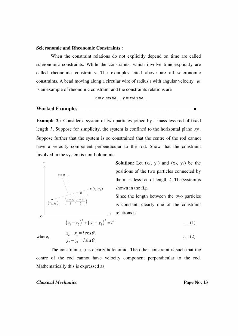
Example 2 : Consider a system of two particles joined by a mass less rod of fixed
length l . Suppose for simplicity, the system is confined to the horizontal plane xy .
Suppose further that the system is so constrained that the centre of the rod cannot
have a velocity component perpendicular to the rod. Show that the constraint
involved in the system is non-holonomic.
Solution: Let (x1, y1) and (x2, y2) be the
positions of the two particles connected by
the mass less rod of length l . The system is
shown in the fig.
Since the length between the two particles
is constant, clearly one of the constraint
relations is
( ) ( )2 2 2
1 2 1 2x x y y l− + − = . . . (1)
where, 2 1
2 1
cos ,
sin
x x l
y y l
θ
θ
− =
− = . . . (2)
The constraint (1) is clearly holonomic. The other constraint is such that the
centre of the rod cannot have velocity component perpendicular to the rod.
Mathematically this is expressed as
Ox
y
θ
v = 0
( )1 1,x y
( )2 2,x y
1 2 1 2,2 2
x x y y+ +
Page 14
Classical Mechanics Page No. 14
( ) ( ) ( )1 2 1 2cos 90 cos 0x x y yθ θ+ + + + =� � � � ,
( ) ( )1 2 1 2sin cosx x y yθ θ+ = +� � � � . . . . (3)
This constraint can not be integrated and hence the constraint is non-holonomic and
consequently, the system is non-holonomic.
• Degrees of freedom and Generalized co-ordinates :
Consider the motion of a free particle. To describe its motion we need three
independent co-ordinates, such as the Cartesian co-ordinates x, y, z or the spherical
polar co-ordinates , ,r θ φ etc. The particle is free to execute motion along any one of
the axes independently with change in only one co-ordinate. In this case we say that
the particle has three degrees of freedom. Thus we define
Definition : The least possible number of independent co-ordinates required to
specify the motion of the system completely by taking into account the constraints is
called degrees of freedom.
e.g. For a system of N particles free from constraints moving independent of each
other has 3N degree of freedom.
Generalized co-ordinates:
A system of N particles free from constraints has 3N degrees of freedom. If
however, there exists k holonomic constraints expressed in k equations
( )1 2, ,..., , 0, 1,2,...,i nf r r r t i k= = , . . . (1)
then 3N co-ordinates are not all independent but related by k equations given in (1).
We may use these k equations to eliminate k of the 3N co-ordinates, and we are left
with 3N k n− = (say) independent co-ordinates. These are generally denoted by
, 1, 2,...,j
q j n= called the generalized co-ordinates and the system has 3N-k
degrees of freedom.
Page 15
Classical Mechanics Page No. 15
Definition: A set of linearly independent variables 1 2 3, , ,...n
q q q q that are used to
describe the configuration of the system completely by taking into account the
constraints forces acting on it is called generalized co-ordinates.
Thus in general we have
No. of degrees of freedom – No. of constraints= No. of generalized co-ordinates.
Note: The generalized co-ordinates need not be the position co-ordinates, which have
the dimensions of length, breath and height, but they can be angles, charges or
momentum of the particle.
• Transformation Relations:
It is always possible to express the position co-ordinates of a particle or a
system of particles in terms of generalized co-ordinates and vice-versa. This
expression is called the transformation relation.
e.g., If , 1,2,3,...i
r i n= are the position vectors of the n particles of the system and
, 1,2,...,j
q j n= are the generalized co-ordinates, then there exists a relation
( )1 2 3, , ,... ,i i nr r q q q q t= , . . . (1)
called the transformation relation.
Work: Let a force F be acted on a particle whose position vector is r . Suppose the
particle is displaced through an infinitesimal distance dr due to the application of
force F. Then the work done by the force F is given by
dW F dr=
If the particle is finitely displaced from point ( )1P r to ( )2P r along any path, then
the work done by F is given by
2
1
r
r
W F dr= ∫ . . . (1)
Conservative Force : The work given in expression (1) is in general depends on the
extreme positions of the particle and also the path along which it travels. If a force is
Page 16
Classical Mechanics Page No. 16
such that the work depends only upon the positions 1P , 2P and not on the path
followed by the particle, then the force F is called conservative force, otherwise non-
conservative.
Worked Examples •
Example 3 : Show that the gravitational force is conservative.
Solution : Let a particle of mass m move along a curve PQ under gravity. Thus the
only force acting on the particle is its own
weight in the down ward direction. Therefore,
work done by the force is given by
Q
P
W F dr= ∫ ,
If F Xi Yj= + and r xi yj= + , where X and Y
are the components of the force along the co-
ordinate axes. We see that 0X = , and Y w= − .
Hence
b
a
W wdy= −∫ ,
where a and b are the ordinates at points P and Q respectively.
This implies
( )W w a b= − .
This shows that the work does not depend upon the path but depends on the
extreme points. Hence the gravitational force is conservative. Alternately, we say
that, the force F is conservative if the work done by it around the closed path is zero.
i. e. F is conservative iff 0F dr =∫� . . . (1)
However, by Stokes theorem, we have
. ,s
F dr F ds= ∇×∫ ∫� . . . (2)
Ox
z
X
YP
Q
ab
W = mg
Page 17
Classical Mechanics Page No. 17
where ds is an arbitrary surface element. Thus from equations (1) and (2) we have
F is conservative iff 0F∇× = . . . (3)
However, 0F F∇× = ⇒ is a gradient of some potential V.
V
F V or Fr
∂⇒ = −∇ = −
∂,
where V is a potential called potential energy of the particle and is a function of
position only. Thus the force F is conservative if
F V= −∇ . . . (4)
and conversely. The negative sign indicates that F is in the direction of decreasing V.
Example 4: Show that the inverse square law of attractive force (central force) is
conservative.
Solution: The inverse square law of force is the force of attraction between two
particles and is given by
1 2
2
m mF G
r= − . . . (1)
where negative sign indicates that the force is directed towards the fixed point and it
is called the attractive force. We write the force as
1 23,
kF r for k Gm m
r= − = . . . (2)
For r xi yj zk= + +
We have ( )
( )3
2 2 2 2
k xi yj zkF
x y z
+ += −
+ +
. . . (3)
For conservative force we have 0F∇× = .
Page 18
Classical Mechanics Page No. 18
Consider therefore
3 3 3
3 3 3 3 3 3.
i j k
Fx y z
Kx Ky Kz
r r r
z y x z y xF K i j k
y r z r z r x r x r y r
∂ ∂ ∂∇× =
∂ ∂ ∂
− − −
∂ ∂ ∂ ∂ ∂ ∂ ∇× = − − + − + −
∂ ∂ ∂ ∂ ∂ ∂
5 5 5 5 5 5
2 2 2 2 2 2
3 3 3 3 3 3.
0.
yz yz xz xz yx yxF K i j k
r r r r r r
F
− − − ∇× = − + + + + +
∇× =
This shows that the inverse square law of attractive force F is conservative.
••
• Virtual Work :
If the system of forces acting on a particle be in equilibrium then their
resultant is zero and hence the work done is zero.
Thus in the case of a particle be in equilibrium there is no motion, hence there
arises no question of displacement. In this case we assume the particle receives a
small virtual displacement (the displacement of the system which causes no real
motion is called as virtual or imaginary displacement) and it is denoted by i
rδ .
Virtual displacement i
rδ is assumed to take place only in the co-ordinates and at
fixed instant t, hence δ change in time t is zero.
( )i i dt or drδ
== .
Thus the work done by the system of forces in causing imaginary
displacement is called virtual work. It is the amount of work that would have been
Page 19
Classical Mechanics Page No. 19
done if the actual displacement had been caused. Hence the expression for the virtual
work done by the forces is given by
Virtual work i i
i
W F rδ δ=∑ . . . . (1)
• Principle of Virtual Work :
If the forces are in equilibrium then the resultant is zero. Hence the algebraic
sum of the virtual work is zero. Conversely, if the algebraic sum of the virtual work
is zero then the forces are in equilibrium.
Note that this principle is applicable in statics. However, an analogous
principle in dynamics was put forward by D’Alembert.
• D’Alembert’s Principle :
D’Alembert started with the equation of motion of a particle i i
F p= � , where
ip is the linear momentum of the th
i particle. This can be written as 0i i
F p− =� .
Hence ( ) 0,i i
i
F p− =∑ �
implying a system of particles is in equilibrium. This equation states that the
dynamical system appears to be in equilibrium under the action of applied forces i
F
and an equal and opposite ‘effective forces’i
p� . In this way dynamics reduces to
static. Thus
( ) 0i i
i
F p− = ⇔∑ � the system is in equilibrium (the resultant is zero).
Hence the virtual work done by the forces is zero. This implies that
( ) 0i i i
i
F p rδ− =∑ � .
This is known as the mathematical form of D’Alembert principle. This states that “a
system of particles moves in such a way that the total virtual work done by the
applied forces and reverse effective forces is zero’’.
Page 20
Classical Mechanics Page No. 20
Note :
1. D’Alembert Principle describes the motion of the system by considering its
equilibrium.
2. All the laws of mechanics may be derived from this single principle. Hence
D’Alembert principle has been called the fundamental principle of
mechanics. We will solve some examples by using this principle.
Worked Examples •
Example 5: A particle is constrained to move in a circle in a vertical plane xy. Apply
the D’Alembert’s principle to show that for equilibrium we must
have 0xy yx gx− − =�� �� .
Solution: Consider a particle of mass m be moving along
a circle of radius r in xy plane. Let (x, y) be the position
of the particle at any instant t with respect to the fixed-
point 0.The constraint on the motion of the particle is that
the position co-ordinates of the particle always lie on the
circle. Hence the equation of the constraint is
2 2 2x y r+ = . . . (1)
2 2 0x x y yδ δ⇒ + =
or y
x yx
δ δ= − . . . (2)
where xδ and yδ are displacement in x and y respectively. Now from
D’Alembert’s principle, we have
( ) 0F mr rδ− =�� .
In terms of components we have
( ) ( ) 0x y
F mx x F my yδ δ− + − =�� �� . . . . (3)
(x, y)
W = mg
O
Page 21
Classical Mechanics Page No. 21
However, the only force acting on the particle at any instant t is its weight mg in the
downward direction. Resolving the force horizontally and vertically, we have 0x
F =
and y
F mg= − . Therefore equation (3) becomes
( ) 0mx x mg my yδ δ− − + =�� �� .
On using (2) we have
( ) 0m xy yx gx xδ− + + =�� �� .
For 0, 0x and mδ ≠ ≠ we have
0xy yx gx− − =�� �� , . . . (4)
which is the required equation of motion.
Example 6: Use D’Alembert’s principle to determine the equation of motion of a
simple pendulum.
Solution : Consider a particle of mass m attached to one end of the string and other
end is fastened to a fixed point 0. Let l be
the length of the pendulum and θ the
angular displacement of the pendulum
shown in the fig.
According to the D’Alembert’s principle we
have
( ) 0i i i
i
F p rδ− =∑ �
where i is the number of particles in the system.
( ) 0F mr rδ⇒ − =�� ,
where r is the distance of the particle from the starting point along the curve.
Resolving the force acting on the particle along the direction of motion and
perpendicular to the direction of motion we have
B(x, y)
mg
mg sin θ
y
A
O x
mg cos θ
θl
Page 22
Classical Mechanics Page No. 22
( )sin 0mg mr rθ δ− − =�� ,
where the negative sign indicates the force is opposite to the direction of motion.
Since 0rδ ≠ we have
sinr g θ= −�� . . . . (1)
From the figure we have r = arcAB r lθ⇒ = r lθ⇒ = ���� .
Equation (1) becomes
sing
lθ θ= −�� . . . . (2)
For small angle, we have sing
lθ θ θ θ= ⇒ = −�� .
••
• Generalized Velocities :
From transformation equations we have
( )1 2 3, , ,... ,i i nr r q q q q t= , . . . (1)
Differentiating this with respect to t we get
i ij
j j
r rr q
q t
∂ ∂= +
∂ ∂∑� � . . . (2)
where , 1, 2,3,...,j
q j n=� are called generalized velocities.
• Virtual displacement :
We find δ variation (change) in the transformation equation (1) to get
ii j
j
rr q
qδ δ
∂=
∂∑
Note here that tδ term is absent because virtual displacement is assumed to take
place at fixed instant t, hence 0tδ = .
Page 23
Classical Mechanics Page No. 23
• Generalized force :
If i
F are forces acting on a dynamical system with position vectors i
r then
virtual work done by these forces is given by
,
,
,
,
i i
i
ii j
i j j
ii j
j i j
j j
j
W F r
rF q
q
rF q
q
Q q
δ δ
δ
δ
δ
=
∂=
∂
∂= ∂
=
∑
∑∑
∑ ∑
∑
where
ij i
i j
rQ F
q
∂=
∂∑ . . . (1)
are called the components of generalized forces.
Note :
1. If forces are conservative then they are derived from potential V and are
given by
i i
i
VF V
r
∂= −∇ = −
∂.
Consequently, the generalized forces are given by j
j
VQ
q
∂= −
∂.
2. If the forces are non-conservative, the scalar potential U may be function of
position, velocity and time. i.e., ( ), ,j j
U U q q t= � . This is called velocity dependent
potential or generalized potential. Such a potential exits in the case of a motion of a
particle of charge q moving in an electromagnetic field. We will see latter in example
(8) that how the generalized potential can be determined in the case of a particle
moving in an electromagnetic field. In this case generalized forces are given by
Page 24
Classical Mechanics Page No. 24
j
j j
U d UQ
q dt q
∂ ∂= − + ∂ ∂ �
.
3. If however, the system is acted upon by conservative forces i
F and non-
conservative forces ( )d
iF , in this case generalized forces
jQ are given by
( )( ) ( )d di
j i i j j
j j
r VQ F F Q Q
q q
∂ ∂= + ⇒ = − +
∂ ∂∑ ,
where
( ) ( )d d ij i
i j
rQ F
q
∂=
∂∑
are non-conservative forces which are not derivable from the potential V. Such a
situation often arises when frictional forces or dissipative forces are present in the
system.
It is found by experiment that in general the dissipative or frictional forces are
proportional to the velocity of the particle.
( )d
i i iF rλ⇒ = − � ,
where i
λ are constants. In such cases the generalized forces are obtained as
( ) ( ),
d d ij i
i j
ii i
i j
rQ F
q
rr
qλ
∂=
∂
∂= −
∂
∑
∑ �
However, from transformation equation we obtain
i i
j j
r r
q q
∂ ∂=
∂ ∂
�
�.
Thus we write
( ) 21,
2
,
d
j i i
j
j
Q rq
R
q
λ∂
= − ∂
∂= −
∂
∑ �
�
�
Page 25
Classical Mechanics Page No. 25
where 21
2i i
R rλ= ∑ �
is called the Rayleigh’s dissipative function.
Unit 2: Lagrange’s Equations of motion:
Newtonian approach for the description of particle involves vector quantities.
We now introduce another formulation called the Lagrangian formulation for the
description of mechanics of a particle or a system of particles in terms of generalized
coordinates, generalized velocities with time t as a parameter. This formulation
involves scalar quantities such as kinetic energy and the potential energy and hence
proves to be easier then the Newtonian approach, because to deal with scalars is easy
than to deal with vectors.
• Lagrange’s Equations of motion from D’Alembert’s Principle :
Theorem 3 : Obtain Lagrange’s equations of motion from D’Alembert’s principle.
Proof : Consider a system of n particles of masses i
m and position vectors i
r . We
know the position vectors i
r are expressed as the functions of n generalized co-
ordinates 1 2 3, , ,...,n
q q q q and time t as
( )1 2 3, , ,... ,i i nr r q q q q t= , . . . (1)
If i
F are the forces acting on the system, then by D’Alembert’s principle we have
( ) 0i i i
i
F p rδ− =∑ � , . . . (2)
where, i i i
p m r=� �� is the linear momentum of the thi particle of the system . From the
transformation equations we obtain the expression for the virtual displacement
ii j
j
rr q
qδ δ
∂=
∂∑ ,
Page 26
Classical Mechanics Page No. 26
where the term tδ is absent because the virtual displacement is assumed to take
place only in the co-ordinates and at the particular instant. Hence equation (2)
becomes
i ii j i i j
i j i jj j
r rF q m r q
q qδ δ
∂ ∂=
∂ ∂∑∑ ∑∑ �� .
,
i ii j i i j
j i i jj j
r rF q m r q
q qδ δ
∂ ∂= ∂ ∂
∑ ∑ ∑ �� ,
or ,
ij j i i j
j i j j
rQ q m r q
qδ δ
∂=
∂∑ ∑ �� , . . . (3)
where
,i
i
j
rQ F
q
∂=
∂∑ . . . . (4)
are called the components of generalized forces.
Consider
i i ii i i
j j j
r r rd dr r r
dt q q dt q
∂ ∂ ∂= + ∂ ∂ ∂
� �� � .
Substituting this in equation (3) we get
,
i ij j i i i j
j i j j j
r rd dQ q m r r q
dt q dt qδ δ
∂ ∂= − ∂ ∂
∑ ∑ � � . . . . (5)
Now from equation (1) we have
i ii k
k k
r rr q
q t
∂ ∂= +
∂ ∂∑� � . . . . (6)
Differentiating this with respect to j
q� we get
i i
j j
r r
q q
∂ ∂=
∂ ∂
�
�. . . . (7)
Further, differentiating equation (6) w. r. t. j
q , we get
Page 27
Classical Mechanics Page No. 27
2 2
i i ik
kj k j j
r r rq
q q q t q
∂ ∂ ∂= +
∂ ∂ ∂ ∂ ∂∑
�� . . . . (8)
Also we have
2 2
i i ik
kj j k j
r r rdq
dt q q q q t
∂ ∂ ∂= + ∂ ∂ ∂ ∂ ∂ ∑ � . . . . (9)
We notice from equations (8) and (9) that
i i
j j
r rd
q dt q
∂ ∂= ∂ ∂
�
In general we have
j j
d d
q dt dt q
∂ ∂ = ∂ ∂
. . . . (10)
On using equation (10) in equation (5) we get
,
i ij j i i i i j
j i j j j
v vdQ q m v m v q
dt q qδ δ
∂ ∂= − ∂ ∂
∑ ∑�
.
We write this as
2 21 1
2 2j j i i i i j
j j i ij j
dQ q m v m v q
dt q qδ δ
∂ ∂ = − ∂ ∂
∑ ∑ ∑ ∑�
,
or j j j
j j j j
d T TQ q q
dt q qδ δ
∂ ∂= − ∂ ∂
∑ ∑�
,
where 21
2i i
i
T m v= ∑
is the total kinetic energy of the system of particles.
0j j
j j j
d T TQ q
dt q qδ
∂ ∂⇒ − − = ∂ ∂
∑�
. . . . (11)
Page 28
Classical Mechanics Page No. 28
If the constraints on the motion of particles in the system are holonomic then j
qδ are
independent. In this case we infer from equation (11) that
0j
j j
d T TQ
dt q q
∂ ∂− − = ∂ ∂ �
,
, 1, 2,3,....,j
j j
d T TQ j n
dt q q
∂ ∂− = = ∂ ∂ �
. . . . (12)
These are called the Lagrange’s equations of motion. We see that, to derive
the Lagrange’s equations of motion the knowledge of forces acting on the system of
particles will not be necessary.
Note : If the constraints are non-holonomic then the generalized co-ordinates are not
all independent of each other. Hence we can’t conclude equation (12) from equation
(11).
Note: In deriving Lagrange’s equations of motion the requirement of holonomic
constraints does not appear until the last step.
Case (1) : Conservative system :
If the system is conservative so that particles move under the influence of a
potential which is dependent on co-ordinates only, then the forces are derived from
the potential V given by
i i
i
VF V
r
∂= −∇ =
∂.
In this case the components of generalized forces becomes
ij
i i j j
rV VQ
r q q
∂∂ ∂= =
∂ ∂ ∂∑ , and ( )j
V V q≠ � .
Hence equation (12) becomes
( ) ( )
0j j
d T V T V
dt q q
∂ − ∂ −− = ∂ ∂ �
.
Define a new function L T V= − ,
Page 29
Classical Mechanics Page No. 29
where L which is a function of 1 2 3 1 2 3, , ,..., , , , ,...,n n
q q q q q q q q� � � � and time t is called a
Lagrangian function of the system of particles. Then the equations of motion become
0j j
d L L
dt q q
∂ ∂− = ∂ ∂ �
. j = 1, 2, ..., n . . . (13)
These are called the Lagrange’s equations for motion for conservative holonomic
system.
Note : The Lagrangian L satisfying equation (13) is not unique. Refer Example (13)
bellow.
Case (2) : Non-conservative system :
In the case of non-conservative system the scalar potential U may be
function of both position and velocity. i.e., ( ), ,j j
U U q q t= � . Such a potential is
called as velocity dependent potential. In this case the associated generalized forces
are given by
j
j j
U d UQ
q dt q
∂ ∂= − + ∂ ∂ �
.
Substituting this in the equation (12) we get
0j j
d L L
dt q q
∂ ∂− = ∂ ∂ �
, 1, 2,...,j n=
which are the Lagrange’s equations of motion for non-conservative forces.
Case (3) : Partially conservative and partially non-conservative system :
Consider the system is acted upon by conservative forces i
F and non-
conservative forces( )d
iF . Such a situation often occurs when frictional forces or
dissipative forces are present in the system. In this case the components of
generalized force are given by
Page 30
Classical Mechanics Page No. 30
( )( ) ( )d di
j i i j j
j j
r VQ F F Q Q
q q
∂ ∂= + ⇒ = − +
∂ ∂∑ ,
where the non-conservative forces which are not derivable from potential function V
are represented in ( )d
jQ . Substituting this in equation (12) we readily obtain
( )d
j
j j
d L LQ
dt q q
∂ ∂− = ∂ ∂ �
, 1, 2,...,j n= . . . (14)
where the Lagrangian L contains the potential of the conservative forces, and ( )d
jQ
represents the forces not arising from the potential V. However, it is found by
experiment that, in general the dissipative or frictional forces are proportional to the
velocity of the particles.
( )d
i i iF rλ= − � ,
iλ are constants.
Hence we have
( ) ( ),
.
d d ij i
i j
ii i
i j
rQ F
q
rr
qλ
∂=
∂
∂= −
∂
∑
∑ �
But we know that
i i
j j
r r
q q
∂ ∂=
∂ ∂
�
�.
Hence
( ) 21
2
d
j i i
j j
RQ r
q qλ
∂ ∂ = − = −
∂ ∂ ∑ �
� � ,
where 21
2i i
i
R rλ= ∑ �
is called Rayleigh’s dissipation function. Hence the Lagrange’s equations of motion
become
Page 31
Classical Mechanics Page No. 31
0j j j
d L L R
dt q q q
∂ ∂ ∂− + = ∂ ∂ ∂ � �
. . . . (15)
Worked Examples •
• Conservation of Energy:
Example 7: Show that the total energy of a particle moving in a conservative force
field remains constant, if the potential energy is not an explicit function of time.
Solution : Let a particle of mass m be moving in the conservative field of force F.
Let r be the position vector of the particle at any instant. The total energy of the
particle is
E T V= + , . . . (1)
where T = kinetic energy,
V = potential energy.
Differentiating (1) with respect to t we get
dE dT dV
dt dt dt= + , . . . (2)
where the force
dv
F mdt
=
Therefore
,
dv drFdr m dt
dt dt
Fdr mvdv
=
=
21
2
,
Fdr d mv
Fdr dT
=
⇒ =
dr dT
Fdt dt
⇒ = . . . . (3)
Page 32
Classical Mechanics Page No. 32
Similarly, we have the potential energy V =V(r, t), therefore,
V V V V
dV dx dy dz dtx y z t
∂ ∂ ∂ ∂= + + +
∂ ∂ ∂ ∂,
.V
dV V dr dtt
∂⇒ = ∇ +
∂,
.dV dr V
Vdt dt t
∂⇒ = ∇ +
∂. . . . (4)
Substituting this in equation (2) we get
dE dr dr V
F Vdt dt dt t
∂= + ∇ +
∂,
( )dE dr V
F Vdt dt t
∂= + ∇ +
∂.
Since F is conservative
,
.
F V
dE V
dt t
⇒ = −∇
∂⇒ =
∂
Now if the potential energy V is independent of time t then
0dE
dt= .
This implies that E is conserved.
••
Theorem 4 : If the force acting on a particle is conservative then the total energy is
conserved.
Proof : If the particle is acted upon by the force F, then if it moves from position 1P
to 2P . Hence the work done by the force is given by
2
1
.
P
P
W F dr= ∫ . . . (1)
where dv
F p mdt
= =� ,
Page 33
Classical Mechanics Page No. 33
Therefore,
2 2
1 1
2
1
2
1
2
2
2 2
2 1
. .
1,
2
1,
2
1 1.
2 2
P P
P P
P
P
P
P
dv dr dvW m dt m v dt
dt dt dt
dmv dt
dt
mv
W mv mv
= =
=
=
= −
∫ ∫
∫
Thus 2 1W T T= − . . . . (2)
Now, if the force F is conservative then it is derivable from a scalar potential
functionV , which is a function of position only. Therefore, we have
,V
F Vr
∂= −∇ = −
∂ where V is the potential energy. Substituting this value in
equation (1) we get
2
1
P
P
VW dr
r
∂= −
∂∫,
2
1
P
P
dV= −∫ ,
( ) 2
1
P
PV= − ,
1 2W V V= − . . . . (3)
From equations (2) and (3) we have
2 1 1 2T T V V− = −
1 1 2 2T V T V+ = + = constant
T V⇒ + = constant.
This shows that the total energy of the particle is conserved.
Page 34
Classical Mechanics Page No. 34
Aliter : The force field is conservative. This implies that
F V= −∇ , . . . (1)
where V is the potential energy. Newton’s second law of motion defines the force by
F mr= �� . . . . (2)
Thus we have
V
mrr
∂= −
∂�� .
Multiply this equation by r� , we get
V
mr r rr
∂= −
∂�� � � .
This we write as
210
2
dmr V
dt
+ =
� .
Integrating we get
21.
2mr V const+ =�
This shows that the total energy of the particle moving in the conservative field of
force is constant.
Theorem 5 : If the external and internal forces are both conservative, then show that
the total potential energy V of the system is given by
( ) ( )int
,
1
2
e
i ij
i i j
V V V= +∑ ∑ ,
where ( )e
iV is the potential energy arises due to the external forces
( )e
iF and
( )int
ijV is
the internal energy arises due to internal forces ( )int
jiF . Further show that the total
energy of the system is conserved.
Page 35
Classical Mechanics Page No. 35
Proof : Two types of forces viz., external and internal forces are acting on the system
of particles. To find the total energy of the system, we find the work done by all the
forces external as well as internal in moving the system from initial configuration 1
to the final configuration 2. It is given by
2
1
i i
i
W F dr=∑∫ ,
where
( ) ( )inte
i i ji
j
F F F= +∑
( ) ( )
2 2int
, ,1 1
e
i i ji i
i i j i j
W F dr F dr≠
⇒ = +∑ ∑∫ ∫ . . . (1)
Let ( )e
iF be conservative, then there exists a potential
( )e
iV such that
( ) ( )
( )ee e i
i i i
i
VF V
r
∂= −∇ = −
∂
( )
( )( )
2 2 2
1 1 1
,
ee ei
i i i i
i i ii
VF dr dr dV
r
∂= − = −
∂∑ ∑ ∑∫ ∫ ∫
( ) ( )
22
1 1
e e
i i i
i i
F dr V
= −
∑ ∑∫ . . . (2)
Now consider the second term on the r. h. s. of equation (1)
( ) ( )
2 2int int
, , , ,1 1
ji i ji i
i j i j i j i j
F dr F dr≠ ≠
=∑ ∑∫ ∫ . . . (3)
Interchanging i and j on the r. h. s. of equation (3) we get
( ) ( )
2 2int int
, , , ,1 1
ji i ij j
i j i j i j i j
F dr F dr≠ ≠
=∑ ∑∫ ∫
( ) ( )
2 2int int
, , , ,1 1
ji i ji j
i j i j i j i j
F dr F dr≠ ≠
= −∑ ∑∫ ∫ (( ) ( )int int
ji ijF F= − ) . . . (4)
Adding equations (3) and (4) we get
Page 36
Classical Mechanics Page No. 36
( ) ( ) ( )
( ) ( )
2 2int int
, , , ,1 1
2 2int int
, , , ,1 1
1
2
1,
2
ji i ji i j
i j i j i j i j
ji i ji ij ij i j
i j i j i j i j
F dr F dr dr
F dr F dr for dr dr dr
≠ ≠
≠ ≠
= −
= = −
∑ ∑∫ ∫
∑ ∑∫ ∫
Now if the internal forces ( )int
jiF are conservative, there exists a potential ( )int
ijV such
that
( ) ( )
( )int
int int ij
ji ji ji
ij
VF V
r
∂= −∇ = −
∂,
where ji
∇ is the gradient with respect to ji
r . Thus the above equation becomes
( )
( )int2 2int
, , , ,1 1
1
2
ij
ji i ij
i j i j i j i j ij
VF dr dr
r≠ ≠
∂= −
∂∑ ∑∫ ∫ ,
( ) ( )
2 2int int
, , , ,1 1
1
2ji i ij
i j i j i j i j
F dr dV≠ ≠
= −∑ ∑∫ ∫ ,
( ) ( )
22
int int
, , ,1 1
1
2ji i ij
i j i j i j
F dr V≠
= −
∑ ∑∫ . . . . (5)
Substituting the values from equations (2) and (5) we get
[ ]2
1 21W V V V= − = − , . . . (6)
where
( ) ( )int
,
1
2
e
i ij
i i j
V V V= +∑ ∑ . . . (7)
represents the total potential energy of the system of particles. Similarly the total
work done by the force on the system in terms of kinetic energy is given by
Page 37
Classical Mechanics Page No. 37
( )
1
2
1
2
1
2
,
i i
i
ii i
i
ii i
i
W F dr
drdW m v dt
dt dt
dvm v dt
dt
=
=
=
∑∫
∑∫
∑∫
1
2
2
2
2
1
1
2
1
2
i i
i
i i
i
dW m v dt
dt
W d m v
=
=
∑∫
∑∫
2
2
2 1
1
1
2i i
i
W m v T T
= = −
∑ . . . (8)
From equations (6) and (8) we have
1 1 2 2T V T V+ = + .
This shows that the total energy of the system is conserved.
Example 8 : Find the velocity dependent potential and hence the Lagrangian for a
particle of charge q moving in an electromagnetic field.
Solution : Consider a charge particle of charge q moving with velocity v in an
electric field E and magnetic field B . The force acting on the particle is called
Lorenz force and is given by
( )F q E v B= + × , . . . (1)
where E and B satisfy the Maxwell’s field equations
0,
.
B
BE
t
∇ ⋅ =
∂∇× = −
∂
. . . (2)
Page 38
Classical Mechanics Page No. 38
We know the vector identity 0A∇ ⋅∇× = . Thus the Maxwell equation implies that
there exists the magnetic vector potential A which is a function of co-ordinates and
velocities such that
B A= ∇× . . . . (3)
Substituting this in the second Maxwell equation we get
( ) 0,
0,
E At
AE
t
∂∇× + ∇× =
∂
∂⇒ ∇× + ∇× =
∂
0A
Et
∂⇒ ∇× + =
∂ . . . . (4)
We also know the vector identity
0φ∇×∇ = . . . (5)
Comparing equations (4) and (5) we see that, there exists a scalar potential φ which
is function of co-ordinates and not involving velocities such that
A
Et
φ∂
+ = −∇∂
A
Et
φ∂
⇒ = −∇ −∂
. . . (6)
Using equations (3) and (6) in equation (1) we get
A
F q v At
φ ∂
= −∇ − + ×∇× ∂ . . . (7)
where we have
,i j kx y z
φ φ φφ
∂ ∂ ∂∇ = + +
∂ ∂ ∂
,yx z
AA AAi j k
t t t t
∂∂ ∂∂= + +
∂ ∂ ∂ ∂
Page 39
Classical Mechanics Page No. 39
,y yx xz z
x y z
y y yx x xz zy z x z
x zx
i j k
A AA AA AA i j k
x y z y z z x x y
A A A
A A AA A AA Av A i v v j v v
x y z x x y y z
A Ak v
z x
∂ ∂ ∂ ∂∂ ∂∂ ∂ ∂ ∇× = = − + − + −
∂ ∂ ∂ ∂ ∂ ∂ ∂ ∂ ∂
∂ ∂ ∂ ∂ ∂ ∂∂ ∂ ×∇× = − − − + − − − +
∂ ∂ ∂ ∂ ∂ ∂ ∂ ∂
∂ ∂ + −
∂ ∂
yzy
AAv
y z
∂ ∂− −
∂ ∂
Therefore the x-component of the Lorentz force (7) becomes
yx x x z
x y z
AA A A AF q v v
x t x y z x
φ ∂ ∂ ∂ ∂ ∂∂ = − − + − − −
∂ ∂ ∂ ∂ ∂ ∂ . . . (8)
Now consider
y yx x x x x xz zy z x y z x y z
A AA A A A A AA Av v v v v v v v
x y z x x x x x y z
∂ ∂ ∂ ∂ ∂ ∂ ∂ ∂∂ ∂ − − − = + + − + +
∂ ∂ ∂ ∂ ∂ ∂ ∂ ∂ ∂ ∂ . . . (9)
Also we have
,x x x x xx y z
dA A A A Av v v
dt x y z t
∂ ∂ ∂ ∂= + + +
∂ ∂ ∂ ∂
x x x x xx y z
A A A dA Av v v
x y z dt t
∂ ∂ ∂ ∂+ + = −
∂ ∂ ∂ ∂ . . . (10)
Also
( ) ( )x x y y z zv A v A v A v A
x x
∂ ∂⋅ = + +
∂ ∂
Page 40
Classical Mechanics Page No. 40
( ) yx zx y z
AA Av A v v v
x x x x
∂∂ ∂∂⋅ = + +
∂ ∂ ∂ ∂ . . . (11)
Substituting from equations (10) and (11) in equation (9) we get
( )y x x x xzy z
A A A dA AAv v v A
x y z x x dt t
∂ ∂ ∂ ∂∂ ∂ − − − = ⋅ − +
∂ ∂ ∂ ∂ ∂ ∂ . . . . (12)
Hence equation (8) becomes
( ) xx
dAF q v A
x dtφ
∂ = − − ⋅ − ∂
. . . (13)
Also
( ) ( )x x y y z z x
x x
v A v A v A v A Av v
∂ ∂⋅ = + + =
∂ ∂
As φ is independent of x
v , therefore we write
( ) x
x
v A Av
φ∂
− ⋅ = −∂
( ) x
x
dAdv A
dt v dtφ
∂⇒ ⋅ − ⋅ = −
∂ . . . (14)
Substituting this in equation (13) we get
( ) ( )x
x
dF q v A v A
x dt vφ φ
∂ ∂= − − ⋅ − − ⋅
∂ ∂ . . . (15)
Define the generalized potential
( )U q v Aφ= − ⋅ . . . (16)
Hence we write equation (15) as
x
U d UF
x dt x
∂ ∂ = − − ∂ ∂ �
for x
x v=� . . . (17)
Hence the Lagrange’s equation of motion
Page 41
Classical Mechanics Page No. 41
x
d T TF
dt x x
∂ ∂ − =
∂ ∂ �
becomes
( ) ( )
0
0.
d T T U d U
dt x x x dt x
T U T Ud
dt x x
d L L
dt x x
∂ ∂ ∂ ∂ − = − +
∂ ∂ ∂ ∂
∂ − ∂ − − =
∂ ∂
∂ ∂ − =
∂ ∂
� �
�
�
where the Lagrangian of the particle L T U= − becomes
( )2 2 21
2L m x y z q q v Aφ= + + − + ⋅� � � . . . . (18)
Example 9: Show that the Lagrange’s equation
j
j j
d T TQ
dt q q
∂ ∂− = ∂ ∂ �
can also be written in the form
2j
j j
T TQ
q q
∂ ∂− =
∂ ∂
�
�.
Solution: The kinetic energy T is in general a function of generalized co-ordinates,
generalized velocities and time. Thus we have
( ), ,j j
T T q q t= � . . . . (1)
Differentiating this w. r. t. t we get
k k
k kk k
dT T T TT q q
dt q q t
∂ ∂ ∂= = + +
∂ ∂ ∂∑ ∑� � ��
� . . . . (2)
Differentiating equation (2) partially w. r. t. j
q� we get
2 2 2
j
k k k
k kj j k k j k j
T T T T Tq q
q q q q q q q tδ
∂ ∂ ∂ ∂ ∂= + + + ∂ ∂ ∂ ∂ ∂ ∂ ∂ ∂ ∑ ∑
�
� ��
� � � � �
Page 42
Classical Mechanics Page No. 42
2 2 2
k k
k kj j k j j k j
T T T T Tq q
q q q q q q q t
∂ ∂ ∂ ∂ ∂= + + +
∂ ∂ ∂ ∂ ∂ ∂ ∂ ∂∑ ∑
�
� ��
� � � � �. . . . (3)
Also we find the expression
2 2 2
k k
k kj k j k j j
d T T T Tq q
dt q q q q q t q
∂ ∂ ∂ ∂= + + ∂ ∂ ∂ ∂ ∂ ∂ ∂ ∑ ∑� ��
� � � � �. . . . (4)
From equations (3) and (4) we have
j j j
T d T T
q dt q q
∂ ∂ ∂− = ∂ ∂ ∂
�
� �. . . . (5)
But it is given that
j
j j
d T TQ
dt q q
∂ ∂= + ∂ ∂ �
.
Consequently equation (5) becomes
j
j j j
T T TQ
q q q
∂ ∂ ∂− + = ∂ ∂ ∂
�
�.
⇒ 2j
j j
T TQ
q q
∂ ∂− =
∂ ∂
�
�.
Example10: A particle of mass M moves on a plane in the field of force given by
ˆ cosr
F i kr θ= − , where k is constant and ˆr
i is the radial unit vector. Show that
angular momentum of the particle about the origin is conserved and obtain the
differential equation of the orbit of the particle.
Solution: Let (x, y) and ( ),r θ be the Cartesian and polar co-ordinates of a particle
of mass M moving on a plane under the action of the given field of force
ˆ cosr
F i kr θ= − , . . . (1)
Since the force is explicitly given, hence the Lagrange’s equation motion
corresponding to the generalized coordinates r and θ are given by
Page 43
Classical Mechanics Page No. 43
d T T
Qdt
θθ θ
∂ ∂ − =
∂ ∂ �, . . . (2)
and r
d T TQ
dt r r
∂ ∂ − =
∂ ∂ �, . . . (3)
where T is the kinetic energy of the particle and is given by
( ) ( )2 2 2 2 21 1
2 2T M x y M r r θ= + = + �� � � , . . . (4)
The components of generalized force along the radial direction and in the direction of
θ are given by
ˆ cos ,
0.
r rQ i kr
Qθ
θ= −
=
Hence equations (1) and (2) become
( )2
2
0,
.
dMr
dt
Mr const
θ
θ
=
⇒ =
�
�
and 2 cos 0Mr Mr krθ θ− + =��� .
This is the equation of motion of the orbit of the particle.
Example 11: Show that the Lagrange’s equation of motion can also be written as
0j
j
L d LL q
t dt q
∂ ∂− − = ∂ ∂
∑ ��
,
Solution: A Lagrangian of a particle is
( ), ,j jL L q q t= � ,
Differentiating this w. r. t. we obtain
j j
j jj j
dL L L Lq q
dt q q t
∂ ∂ ∂= + +
∂ ∂ ∂∑ ∑� ��
� . . . (1)
Consider the expression
Page 44
Classical Mechanics Page No. 44
j j j
j j jj j j
d L d L Lq q q
dt q dt q q
∂ ∂ ∂= + ∂ ∂ ∂
∑ ∑ ∑� � ��
� � � . . . (2)
Subtracting equation (2) from (1) we get
j j
j jj j j
d L L L d LL q q
dt q t q dt q
∂ ∂ ∂ ∂− = + − ∂ ∂ ∂ ∂ ∑ ∑� �
� �. . . . (3)
But from Lagrange’s equation we have,
0j j
d L L
dt q q
∂ ∂− = ∂ ∂ �
. . . . (4)
Consequently, equation (3) becomes
0j
j j
d L LL q
dt q t
∂ ∂− − = ∂ ∂ ∑ �
�.
This is the required form.
Example 12: A particle of mass m moves in a plane under the action of a
conservative force F with components ( )2 2xF k x y= − + , ( )2 2yF k x y= − + , k is a
constant. Find the total energy of the motion, the Lagrangian, and the equations of
motion of the particle.
Solution: A particle is moving in a plane. Let (x, y) be the co-ordinates of the
particle at any instant t. If T and V are the kinetic and potential energies of the
particle then we have
( )2 21
2T m x y= +� � , . . . (1)
and ( ),V V x y= . . . . (2)
Since the force is given by
F V= −∇ ,
x y
V V ViF jF i j k
x y z
∂ ∂ ∂⇒ + = − + +
∂ ∂ ∂
Page 45
Classical Mechanics Page No. 45
( ) ( )
( )
( )
2 2
2
2
2 2 ,
2 ,
2 .
V Vk x y i k x y j i j
x y
Vk x y
x
Vk x y
y
∂ ∂− + − + = − +
∂ ∂
∂⇒ = +
∂
∂⇒ = +
∂
We write
V V
dV dx dyx y
∂ ∂= +
∂ ∂,
( ) ( )
( )
2 2
2
2 2 ,
2 ( ) 2 .
dV k x y dx k x y dy
dV k xdx d xy ydy
= + + +
= + +
On integrating we get,
( )2 2 2V k x xy y= + + . . . (3)
The total energy of motion of the particle is therefore given by
E T V= +
While the Lagrangian of the motion is given by
( ) ( )2 2 2 2 21
2L m x y k x xy y= + − + +� � . . . (4)
The Lagrange’s equations of motion corresponding to the generalized co-ordinates x
and y are respectively given by
( )
( )
2
2
2 0,
2 0.
mx k x y
my k x y
+ + =
+ + =
��
��
••
• Kinetic Energy as a Homogeneous Quadratic Function of Generalized
Velocities :
Theorem 6: Find the expression for the kinetic energy as the quadratic function of
generalized velocities. Further show that
Page 46
Classical Mechanics Page No. 46
i) when the constraints are scleronomic, the kinetic energy is a homogeneous
function of generalized velocities and 2j
j j
Tq T
q
∂=
∂∑ �
�,
ii) when the constraints are rheonomic then 2 12j
j j
Tq T T
q
∂= +
∂∑ �
�,
where 1 2,T T have usual meaning.
Proof: Consider a system of particles of masses i
m and position vectors i
r . The
kinetic energy of the system is given by
21
2i i
i
T m r= ∑ � , . . . (1)
where
( )1 2 3, , ,... ,i i nr r q q q q t= ,
i ii k
k k
r rr q
q t
∂ ∂= +
∂ ∂∑� � .
Substituting this value in equation (1) we get
1
2
i i i ii j k
i j kj k
r r r rT m q q
q t q t
∂ ∂ ∂ ∂= + + ∂ ∂ ∂ ∂ ∑ ∑ ∑� �
2
,
1. 2
2
i i i i ii j k j
i j k jj k j
r r r r rT m q q q
q q q t t
∂ ∂ ∂ ∂ ∂ = + +
∂ ∂ ∂ ∂ ∂ ∑ ∑ ∑� � � ,
2
,
1 1
2 2
i i i i ii j k i j i
j k i j i ij k j
r r r r rT m q q m q m
q q q t t
∂ ∂ ∂ ∂ ∂ = + +
∂ ∂ ∂ ∂ ∂ ∑ ∑ ∑ ∑ ∑� � �
or ,
jk j k j j
j k j
T a q q a q a= + +∑ ∑� � � . . . (2)
where 1
,2
i ijk i
i j k
r ra m
q q
∂ ∂=
∂ ∂∑
,i ij i
i j
r ra m
q t
∂ ∂=
∂ ∂∑ ... (3)
Page 47
Classical Mechanics Page No. 47
21
2
ii
i
ra m
t
∂ =
∂ ∑
are definite functions of r and t and hence functions of 'q s and t. From equation (2)
we observe that the kinetic energy is a quadratic function of the generalized
velocities.
Case 1 : If the constraints are scleronomic. This implies equivalently that the
transformation equations do not contain time t explicitly, and then we have
0ir
t
∂=
∂,
and consequently j
a and a vanish. Therefore equation (2) reduces to
,
jk j k
j k
T a q q=∑ � � . . . . (4)
This shows that the kinetic energy is a homogeneous quadratic function of
generalized velocities. Now applying Euler’s theorem for the homogeneous quadratic
function of generalized velocities we have
2j
j j
Tq T
q
∂=
∂∑ �
� . . . (5)
Case 2 : If the constraints are rheonomic then we write equation (2) in the form
2 1 0T T T T= + + , . . . (6)
where
2
,
1
,
,
jk j k
j k
j j
j
T a q q
T a q
=
=
∑
∑
� �
�
. . . (7)
and
2
0
1
2
ii
i
rT a m
t
∂ = =
∂ ∑
are homogeneous function of generalized velocities of degree two, one and zero
respectively.
Page 48
Classical Mechanics Page No. 48
Now we consider
02 1j j j j
j j j jj j j j
TT TTq q q q
q q q q
∂∂ ∂∂= + +
∂ ∂ ∂ ∂∑ ∑ ∑ ∑� � � �
� � � �
On applying Euler’s theorem for the homogeneous function to each term on the right
hand side we readily get
2 12j
j j
Tq T T
q
∂= +
∂∑ �
�. . . . (8)
This completes the proof.
Note : However, the result (8) can also be obtained by direct differentiating equation
(2) w. r. t. j
q� . Thus
2 jk k j
kj
Ta q a
q
∂= +
∂∑ �
�.
Next multiplying this equation by j
q� and summing over j we get
,
2j jk j k j j
j j k jj
Tq a q q a q
q
∂= +
∂∑ ∑ ∑� � � �
�
2 12j
j j
Tq T T
q
∂= +
∂∑ �
�.
The result (5) can similarly be derived by direct differentiating equation (4).
• Another way of proving conservation theorem for energy :
Theorem (7): If the Lagrangian does not contain time t explicitly, the total energy of
the conservative system is conserved.
Proof : Consider a conservative system, in which the forces are derivable from a
potential V which is dependent on position only. The Lagrangian of the system is
defined as
L T V= − , . . . (1)
where
Page 49
Classical Mechanics Page No. 49
( ), ,j j
L L q q t= � . . . (2)
satisfies the Lagrange’s equation
0j j
d L L
dt q q
∂ ∂− = ∂ ∂ �
. . . . (3)
Differentiating equation (2) we obtain
j j
j j j
dL L L Lq q
dt q q t
∂ ∂ ∂= + +
∂ ∂ ∂ ∑ � ��
�.
Since L does not contain time t explicitly implies 0L
t
∂=
∂.
j j
j j j
dL L Lq q
dt q q
∂ ∂= +
∂ ∂ ∑ � ��
�.
On using equation (3) we write
j j
j jj j
dL d L Lq q
dt dt q q
∂ ∂= + ∂ ∂ ∑ ∑� ��
� �.
,
0
j
j j
j
j j
dL d Lq
dt dt q
d LL q
dt q
∂= ∂
∂⇒ − =
∂
∑
∑
�
�
�
�
.
.j
j j
LL q const
q
∂⇒ − =
∂∑ �
�. . . . (4)
Since the potential energy V for the conservative system depends upon the position
co-ordinates only and does not involve generalized velocities. Hence we have
j j
L T
q q
∂ ∂=
∂ ∂� �.
The generalized momentum is defined as
Page 50
Classical Mechanics Page No. 50
j
j
Tp
q
∂=
∂ �.
Thus we have from equation (4) that
( )j j
j
p q L const H− =∑ � . . . . (5)
L does not contain time t means neither the kinetic energy nor the potential energy of
the particle involves time t. In this case the transformation equations do not contain
time t. consequently the constraints are scleronomic. Hence the kinetic energy T is a
homogeneous quadratic function of generalized velocities.
,
jk j k
j k
T a q q=∑ � � . . . (6)
where
1
,2
i ijk i
i j k
r ra m
q q
∂ ∂=
∂ ∂∑
Hence by Euler’s formula we have
2j
j j
Tq T
q
∂=
∂∑ �
� . . . (7)
Hence from equation (4) we have
2T L H− =
2
,
( )
T T V H
T V H
E H Const
⇒ − + =
⇒ + =
⇒ =
This proves the total energy E is conserved for conservative system.
Theorem (8): Show that non-conservation of total energy is directly associated with
the existence of non-conservative forces even if the transformation equation does not
contain time t.
Proof: We know the Lagrange’s equations of motion for a system in which
conservative forces i
F and non-conservative forces ( )d
iF are present are given by
Page 51
Classical Mechanics Page No. 51
( )d
j
j j
d L LQ
dt q q
∂ ∂− = ∂ ∂ �
, j=1, 2, 3, …, n. . . . (1)
where the Lagrangian L contains the potential of the conservative forces and the
forces which are not arising from potential V are represented by ( )d
jQ .
Since ( ), ,j j
L L q q t= �
j j
j j j
dL L L Lq q
dt q q t
∂ ∂ ∂= + +
∂ ∂ ∂ ∑ � ��
�. . . . (2)
From equation (1) we have ( )d
j
j j
L d LQ
q dt q
∂ ∂= − ∂ ∂ �
,
Therefore
( )
( )
,
,
d
j j j j
j j jj j
d
j j j
j jj
dL d L L Lq q Q q
dt dt q q t
d L Lq Q q
dt q t
∂ ∂ ∂= + − + ∂ ∂ ∂
∂ ∂= − + ∂ ∂
∑ ∑ ∑
∑ ∑
� �� �
� �
� �
�
( )d
j j j
j jj
dL d L Lq Q q
dt dt q t
∂ ∂= − + ∂ ∂
∑ ∑� �
� . . . (3)
Since L contains the potential of the conservative forces
This implies that j j
L T
q q
∂ ∂=
∂ ∂� �
( )d
j j j
j jj
dL d T Lq Q q
dt dt q t
∂ ∂= − + ∂ ∂
∑ ∑� �
�. . . . (4)
where T here is a quadratic function of generalized velocities and hence in this case
we have
2j
j j
Tq T
q
∂=
∂∑ �
�. . . . (5)
Substituting this in equation (4) we get
Page 52
Classical Mechanics Page No. 52
( )
2d
j j
j
dL dT LQ q
dt dt t
∂= − +
∂∑ � .
Hence
( )
.d
j j
j
dE LQ q
dt t
∂= −
∂∑ � . . . (6)
If the transformation equations do not contain time t explicitly, then the kinetic
energy does not contain time t. This implies that 0T
t
∂=
∂. Also Lagrangian contains
the potential of conservative forces, we have therefore V=V (j
q ) and hence
0V
t
∂=
∂.
Consequently, we have 0L
t
∂=
∂. Hence equation (6) becomes
( )d
j j
j
dEQ q
dt=∑ � . ...(7)
This shows that the non-conservation of total energy is directly associated with the
existence of non-conservative forces ( )d
jQ . However, if the system is conservative
and the transformation equations do not contain time t then the total energy is
conserved.
Example 13: Show that the new Lagrangian L′ defined by
( ),
jdf q t
L Ldt
′ = + , 1, 2,...,j n=
satisfies Lagrange’s equation of motion, where f is an arbitrary differentiable
functions of j
q and t , and L is a Lagrangian for a system of n degrees of freedom.
Solution : Given that
( ),
jdf q t
L Ldt
′ = + , . . . (1)
Page 53
Classical Mechanics Page No. 53
where L satisfies
0j j
d L L
dt q q
∂ ∂− = ∂ ∂ �
, . . . (2)
We prove that 0j j
d L L
dt q q
′ ′∂ ∂− = ∂ ∂ �
.
Since ( ),j
f f q t= ,
Therefore we have
k
k k
df f fq
dt q t
∂ ∂= +
∂ ∂∑ � . . . . (3)
Differentiating this partially w. r. t. j
q we get
2 2
k
kj k j j
df f fq
q dt q q t q
∂ ∂ ∂ = +
∂ ∂ ∂ ∂ ∂ ∑ � . . . . (4)
Also from equation (3) we have
j j
df f
q dt q
∂ ∂ =
∂ ∂ �.
Differentiating this w. r. t. t we get
2 2
k
kj k j j
d df f fq
dt q dt q q t q
∂ ∂ ∂ = +
∂ ∂ ∂ ∂ ∂ ∑ �
�. . . . (5)
Subtracting equation (4) from (5) we get
0,
. ., 0
j j
j j
d df df
dt q dt q dt
d L Li e
dt q q
∂ ∂ − =
∂ ∂
′ ′∂ ∂− =
∂ ∂
�
�
.
This proves that the Lagrangian of the system is not unique.
Page 54
Classical Mechanics Page No. 54
Example 14 : Deduce the principle of energy from the Lagrange’s equation of
motion.
Solution : We know the Lagrange’s equations of motion are given by
0j j
d L L
dt q q
∂ ∂− = ∂ ∂ �
, . . . (1)
where L T V= − is a Lagrangian and ( ) ( ), ,j j j
V V q T T q q= = �
Hence equation (1) becomes
j j j
d T T V
dt q q q
∂ ∂ ∂− = − ∂ ∂ ∂ �
, . . . (2)
We also know
2j
j j
Tq T
q
∂=
∂∑ �
�. . . . (3)
Also we obtain
j j
j jj j
dT T Tq q
dt q q
∂ ∂= +
∂ ∂∑ ∑� ��
�. . . . (4)
Multiply equation (2) by j
q� and summing over j we obtain
j j j j
j j j jj j j j
d T T T Vq q q q
dt q q q q
∂ ∂ ∂ ∂− − = −
∂ ∂ ∂ ∂ ∑ ∑ ∑ ∑� �� � �
� �. . . . (5)
On using (3) and (4) we write equation (5) as
(2 )d T dT dV
dt dt dt− = − ,
( ) 0,
.
dT V
dt
T V const
⇒ + =
⇒ + =
This implies that total energy is conserved.
••
Page 55
Classical Mechanics Page No. 55
Unit 3: Lagrange’s Equations for Non-holonomic Constraints:
Introduction:
We have seen that the constraints, which are not expressible in the form of
equations are called non-holonomic constraints. We have also seen that this is not the
only way to describe the non-holonomic system. A system is also said to be non-
holonomic, if it corresponds to non-integrable differential equations of constraints.
Such constraints can not be expressed in the form of equation of the type
( ), 0, 1, 2,3,..., .l j
f q t l m= = . . . (1)
Hence such constraints are called non-holonomic constraints. Obviously, holonomic
system has integrable differential equations of constraints expressible in the form of
equation.
Consider non-integrable differential constraints of the type
1
0n
lk k lt
k
a dq a dt=
+ =∑ , . . . (2)
where lk
a and lt
a are functions of j
q and t . Constraints of this type will be
holonomic only if, an integrating factor can be found that turns it in to an exact
differential, and hence the constraints can be reduced to the form of equations.
However, neither equations (2) can be integrated nor one can find an
integrating factor that will turn either of the equations in to perfect differentials.
Hence the constraints cannot be reduced to the form (1). Hence the constraints of the
type (2) are therefore non-holonomic.
Note also that non-integrable differential constraints of the type (2) are not
the only type of non-holonomic constraints. The non-holonomic constraint
conditions may involve higher order derivatives or may appear in the form of
inequalities.
There is no general way of attacking non-holonomic problems. However, the
constraints are not integrable, the differential equations of the constraint can be
introduced in to the problem along with the differential equations of motion and the
Page 56
Classical Mechanics Page No. 56
dependent equations are eliminated by the method of Lagrange’s multipliers. The
method is illustrated in the following theorem.
Theorem 9: Explain the method of Lagrange’s undetermined multipliers to construct
equations of motion of the system with non-holonomic constraints.
Proof: Consider a conservative non-holonomic system, where the equations of the
non-holonomic constraints are given by
1
0n
lk k lt
k
a dq a dt=
+ =∑ , . . . (1)
where l = 1, 2, 3, …., m represents the number of constraints, and lk
a , lt
a are
functions of j
q and t .
Since the constraints are non-holonomic, hence the equations expressing the
constraints (1) cannot be used to eliminate the dependent co-ordinates and hence all
the generalized co-ordinates are not independent, but are related by constraint
relations.
In the variational (Hamilton’s) principle, the time for each path is held fixed
( 0tδ = ). Hence the virtual displacement k
qδ must satisfy the following equations of
constraints.
1
0, 1, 2,3,...,n
lk k
k
a q l mδ=
= =∑ . . . (2)
We can use these m-equations (2) to eliminate the dependent virtual
displacement and reduce the number of virtual displacement to n-m independent one
by the method of Lagrange’s multipliers. Hence we multiply equations (2) by
1 2 3, , , ,m
λ λ λ λ� respectively and summing over l and integrating it between the
limits 0t to 1t we get
1
01 1
0
t m n
l lk k
l kt
a q dtλ δ= =
=∑∑∫ . . . (3)
Page 57
Classical Mechanics Page No. 57
Hamilton’s principle is assumed to hold for non-holonomic system, (see chapter 3)
we therefore have
1
0
0
t
t
Ldtδ =∫ .
1
01
0
t n
k
k k kt
L d Lq dt
q dt qδ
=
∂ ∂⇒ − =
∂ ∂ ∑∫
�. . . . (4)
Adding equations (3) and (4) we get
1
01 1
0
t n m
l lk k
k lk kt
L d La q dt
q dt qλ δ
= =
∂ ∂ − + =
∂ ∂ ∑ ∑∫
� . . . (5)
Note all the virtual displacementk
qδ , 1, 2,...,k n= are not independent but connected
by m equations (2). Now to eliminate the extra dependent virtual displacements we
choose the multipliers 1 2 3, , , ,m
λ λ λ λ� such that the coefficients of m-dependent
virtual displacements, in equation (5) are zero. i.e.,
1
0,m
l lk
lk k
L d La
q dt qλ
=
∂ ∂− + =
∂ ∂ ∑
� for ( ) ( )1 ,..., 1 ,k n m n n= − − − . . . . (6)
Hence from equation (6) we have
1
01 1
0
t n m m
l lk k
k lk kt
L d La q dt
q dt qλ δ
−
= =
∂ ∂ − + =
∂ ∂ ∑ ∑∫
�, . . . (7)
where 1 2 3, , ,...,n m
q q q qδ δ δ δ − are all independent. Hence it follows that
1
0,m
l lk
lk k
L d La
q dt qλ
=
∂ ∂− + =
∂ ∂ ∑
�for 1,2,..., .k n m= − . . . (8)
Combining equations (6) and (8) we have finally the complete set of Lagrange’s
equations of motion for non-holonomic system
1
,m
l lk
lk k
d L La
dt q qλ
=
∂ ∂− =
∂ ∂ ∑
�1,2,..., ,...,k n m n= − . . . . (9)
Page 58
Classical Mechanics Page No. 58
Remarks:
1. The n-equations in (9) together with m-equations of constraints (1) are
sufficient to determine (n + m) unknowns viz., the n-generalized co-ordinates
j
q and m Lagrange’s multipliersl
λ .
2. Lagrange’s multiplier method can also be used for holonomic constraints,
when it is inconvenient to reduce all the 'q s to independent co-ordinates, and
then obtain the forces of constraints.
Worked Examples •
Example 15: Use Lagrange’s undetermined multipliers to construct the equation of
motion of simple pendulum and obtain the force of constraint.
Solution : Consider a simple pendulum of mass m and of constant length l . Let
P (x, y) be the position co-ordinates of the pendulum. Then the equation of the
constraint is
2 2 2x y l+ = . . . . (1)
This shows that x, y are not the generalized co-
ordinates. If ( ),r θ are the polar co-ordinates of
the pendulum, then the equation of constraint is
(say)
1 0f r l≡ − = . . . . (2)
If this constraint is not used to eliminate the dependent variable r, then ,r θ
are the generalized co-ordinates. Hence the kinetic energy and potential energy of the
pendulum are respectively given by
( )2 2 21
,2
cos .
T m r r
V mgr
θ
θ
= +
= −
�
P(x, y)
y
O x
θl
Page 59
Classical Mechanics Page No. 59
The Lagrangian of the pendulum L = T – V becomes
( )2 2 21cos
2L m r r mgrθ θ= + +�� . . . . (3)
Differentiating the equation of the constraint, we get
0dr = .
Comparing this with the standard equation
1 1 0,r
a dr a dθ θ+ = (viz., 0 1, 1,2lk k
k
a dq l k= = =∑ )
we get
1 11, 0r
a a θ= = . . . . (4)
The Lagrange’s equations of motion viz.,
1
,m
l lk
lk k
d L La
dt q qλ
=
∂ ∂− =
∂ ∂ ∑
�1, 2,...,k n=
become 1 1
d L La
dtθλ
θ θ
∂ ∂ − =
∂ ∂ � ,
and 1 1 .r
d L La
dt r rλ
∂ ∂ − =
∂ ∂ �
These equations after solving become
sin 0g
rθ θ+ =�� , . . . (5)
1cosml mgθ θ λ+ = −� , . . . (6)
where 1λ is the force of constraint, in this case it is the tension in the string. Equation
(5) determines the motion of the pendulum under the constraint force given in (6).
Example 16 : Use Lagrange’s undetermined multipliers to construct the equations of
motion of spherical pendulum.
Solution : Let a particle of mass m move on a frictionless surface of radius r under
the action of gravity. Let P (x, y, z) be the position co-ordinates of the pendulum. If
Page 60
Classical Mechanics Page No. 60
( ), ,r θ φ are the spherical polar co-ordinates of the pendulum, then we have the
relations
sin cos ,
sin sin ,
cos ,
x r
y r
z r
θ φ
θ φ
θ
=
=
=
. . . (1)
where 2 2 2 2x y z r+ + = .
This shows that x, y, z are not the generalized
co-ordinates. The kinetic and potential energies
of the spherical pendulum are given by
respectively
( )2 2 2 2 2 21sin ,
2T m r r rθ θφ= + +� �� . . . (2)
cosV mgr θ= . . . . (3)
Hence the Lagrangian of the system becomes
( )2 2 2 2 2 21sin cos
2L m r r r mgrθ θφ θ= + + −� �� . . . . (4)
The equation of the constraint on the motion of the particle moving on the sphere is
1 0f r l≡ − = . . . . (5)
If this constraint is not used to eliminate the dependent variable r, then the
generalized co-ordinates are ( ), ,r θ φ . Differentiating equation (5) we get
0dr =
Comparing this with the standard equation
1 1 0,r
a dr a dθ θ+ = (viz., 0 1, 1,2lk k
k
a dq l k= = =∑ ,3).
we get
1 1 11, 0, 0r
a a aθ φ= = = . . . . (6)
In this case the Lagrange’s equations of motion viz.,
x
y
z
φ
θ
r
z = r cos θ
P(x, y, z) = (r, )θ, φ
Page 61
Classical Mechanics Page No. 61
1
,m
l lk
lk k
d L La
dt q qλ
=
∂ ∂− =
∂ ∂ ∑
�1, 2,...,k n=
become 1 1 ,r
d L La
dt r rλ
∂ ∂ − =
∂ ∂ � . . . (7)
1 1
d L La
dtθλ
θ θ
∂ ∂ − =
∂ ∂ �, . . . (8)
and 1 1
d L La
dtφλ
φ φ
∂ ∂− =
∂ ∂ �. . . . (9)
Consequently, these equations reduce to
2 2 2
1sin cosg
mll
θ θφ θ λ
+ − = − � � . . . . (10)
This equation determines the constraint force. Similarly, from equations (8) and (9)
we obtain
2sin cos sin 0g
lθ θ θφ θ− − =�� � , . . . (11)
and 2 2sin ( .)p constφθφ =� . . . (12)
Eliminating φ� between (11) and (12) we get
2
3cos sin 0
sin
p g
l
φθ θ θθ
− − =�� . . . . (13)
Equations (10) and (13) determine the motion of the spherical pendulum.
Example 17 : A particle is constrained to move on the plane curve xy c= , where c
is a constant, under gravity. Obtain the Lagrangian and hence the equation of motion.
Solution : Given that a particle is constrained to move on the plane curve
xy c= , . . . (1)
The kinetic energy of the particle is given by
( )2 21
2T m x y= +� � . . . (2)
Page 62
Classical Mechanics Page No. 62
The potential energy is given by
,V mgy y is vertical= . . . (3)
We see that x and y are not linearly independent as they are related by the equation
of constraint (1) and hence they are not the generalized co-ordinates. However, we
eliminate the variable y by putting c
yx
= and hence 2
cy x
x= −� � in equations (2) and
(3), we get
22
4
11 ,
2
cT m x
x
cV mg
x
= +
=
�
Here x is the generalized co-ordinate. Hence the Lagrangian of the particle becomes
2
2
4
11
2
c mgcL m x
x x
= + −
� . . . . (4)
The Lagrange’s equation of motion
0d L L
dt x x
∂ ∂ − =
∂ ∂ � ,
becomes
2 2
2
4 5 21 2 0
c c m mgcmx x
x x x
+ − − =
�� � . . . . (5)
Example 18 : A particle is constrained to move on the surface of a cylinder of fixed
radius. Obtain the Lagrange’s equation of motion.
Solution : The surface of the cylinder is characterized by the parametric equations
given by
cos , sin ,x r y r z zθ θ= = = . . . (1)
However, x, y, z are not the generalized co-ordinates as x and y are related by the
equation of constraint 2 2 2x y r+ = , r is a constant radius of the circle. Hence the
Page 63
Classical Mechanics Page No. 63
generalized co-ordinates are θ and z. In terms of these generalized co-ordinates the
kinetic and potential energies become
( )2 2 21
,2
.
T m r z
V mgz
θ= +
=
� �
Hence the Lagrangian is given by
( )2 2 21
2L m r z mgzθ= + −� � . . . . (2)
Therefore the θ − Lagrange’s equation 0d L L
dt θ θ
∂ ∂ − =
∂ ∂ �
yields ( )2 20 ( )d
mr mr const ldt
θ θ= ⇒ =� �
Integrating we get
02
lt
mrθ θ= + , . . . (3)
where 0θ is a constant of integration. Similarly, z- Lagrange’s equation of motion
0d L L
dt z z
∂ ∂ − =
∂ ∂ �,
gives 21
2z ut gt= − , . . . (4)
where 0z u at t= =� .
Example 19 : A particle of mass m is projected with initial velocity u at an angle α
with the horizontal. Use Lagrange’s equation to describe the motion of the projectile.
Solution : Let a particle of mass m be projected from O with an initial velocity u unit
making an angle α with the horizontal line referred as x-axis. Let P (x, y) be the
position of the particle at any instant t. Since x and y are independent and hence the
generalized co-ordinates. The kinetic of the projectile is given by
Page 64
Classical Mechanics Page No. 64
( )2 21
2T m x y= +� � ,
and the potential energy is V mgy=
Thus the Lagrangian function of the
projectile is
( )2 21
2L m x y mgy= + −� � . . . . (1)
The x- Lagrange’s equation of motion and y-Lagrange’s equation of motion
respectively give
0 0x and y g= + =�� �� . . . (2)
To find the velocity of the projectile and its path at any instant we integrate equations
(2) and using boundary conditions we readily obtain
cos , sinx u y u gtα α= = −� � . . . (3)
These equations determine velocity at any time t. Integrating (3) once again and
using boundary conditions we get
21cos . sin .
2x u t and y u t gtα α= = − . . . (4)
Eliminating t between equations (4) we get
2
2 2
1tan
2 cos
xy x g
uα
α= − .. . (5)
This represents the path of the projectile and it is a parabola.
• Atwood’s Machine :
Example 20: Explain Atwood Machine and discuss it’s motion.
mg
x.
= u cosα
y.
= u sin α - gty.
= u sin α
x.
= u cosαOx
y
u
α
Page 65
Classical Mechanics Page No. 65
Solution : Atwood machine consists of two masses 1 2m and m suspended over a
frictionless pulley of radius ‘a’. Both the ends of the string
are attached the masses 1 2m and m respectively. Let the
length of the string between 1 2m and m be l . Then we
have from fig. that PA = x and QA = l - x . The system has
only one degrees of freedom and x is the only generalized
co-ordinate. Hence the kinetic energy of the system is given
by
( ) 2
1 2
1
2T m m x= + � . . . . (1)
Considering the reference level as a horizontal plane
passing through A, the potential energy of both masses is
given by
( )1 2V m gx m g l x= − − − . . . . (2)
Hence the Lagrangian of the system becomes
( ) ( )2
1 2 1 2 2
1
2L m m x m m gx m gl= + + − +� . . . . (3)
The corresponding Lagrange’s equation of motion gives
( )1 2
1 2
m mx g
m m
−=
+�� . . . (4)
The solution of this equation gives
( )1 2 2
0 0
1 2
1
2
m mx gt x t y
m m
−= + +
+ , . . . (5)
where 0 0,x y are constants of integration.
Example 21: A particle of mass m moves in one dimension such that it has the
Lagrangian
m1
m2
m1g
m2g
P
Q
xl - x
a
Page 66
Classical Mechanics Page No. 66
( ) ( )2 4
2 2 ,12
m xL mx V x V x= + −
��
where V is some differentiable function of x. Find equation of motion for x (t).
Solution : Here the Lagrangian of the system is
( ) ( )2 4
2 2 ,12
m xL mx V x V x= + −
�� . . . (1)
We see from equation (1) that x is the only generalized co-ordinate. Therefore the
corresponding Lagrange’s equation of motion becomes
0V
mxx
∂+ =
∂�� . . . . (2)
This equation of motion shows that the particle moves in a straight line under the
action of a force V
Fx
∂= −
∂.
Example 22 : Let a particle be moving in a field of force given by
2
2 2
1 21
r rrF
r c
−= −
� ��.
Find the Lagrangian of motion and hence the equation of motion.
Solution: One can check that 0F∇ × ≠ , hence the force is non-conservative;
consequently, the corresponding potential is generalized potential or velocity
dependent potential. We know the component of generalized force corresponding to
the generalized coordinate r is given by
2
2 2
1 21r
r rrQ F
r c
−= = −
� ��.
We write this force as
2
2 2 2 2
2 2
2 2 2 2 2 2
1 2,
1 2 2,
r
r
r rQ
r c r c r
r r rQ
r c r c r c r
= − +
= + + −
� ��
� �� �
Page 67
Classical Mechanics Page No. 67
2 2
2 2
1 1,r
r d rQ
r r c r dt r r c r
∂ ∂= − + + +
∂ ∂
� �
�
,r
U d UQ
r dt r
∂ ∂= − +
∂ ∂�
2
2
11 .
rU
r c
= +
� …(1)
We notice that the potential energy U is the velocity dependent potential. The
kinetic energy of the particle is given by
21
2T mr= � . ... (2)
Hence the Lagrangian of the particle becomes
2
2
2
1 1 r 1+
2 cL mr
r
= −
�� . ...(3)
We see that r is the only generalized co-ordinate; hence the corresponding
Lagrange’s equation yields the equation of motion in the form
2
2 2 2 2
2 10.
rr m
rc r c r
− + − =
��� …(4)
Example 23 : Derive the equation of motion of a particle falling vertically under the
influence of gravity, when frictional forces obtainable from dissipation function
21
2Kv are present. Integrate the equation to obtain the velocity as a function of time.
Show also that the maximum possible velocity for fall from rest is mg
vK
= .
Solution : Let a particle of mass m be falling vertically under the influence of
gravity. Let z be the height of the particle at any instant t. Therefore the only
generalized co-ordinate is z. Thus the Kinetic energy and the potential energy of the
particle are given by
Page 68
Classical Mechanics Page No. 68
21
2T mz= � . . . (1)
and V mgz= − . . . (2)
Hence the Lagrangian function becomes
21
2L mz mgz= +� . . . . (3)
We know the Lagrange’s equation of motion for a system containing the frictional
forces obtainable from a dissipation function 21
2R Kv= is given by
0d L L R
dt z z z
∂ ∂ ∂ − + =
∂ ∂ ∂ � �. . . . (4)
Solving this equation we get
0mz Kz mg+ − =�� � . . . . (5)
On integrating equation (5) we get
1 0mz Kz mgt c+ − + =� , . . . (6)
where 1c is a constant of integration. Using initial conditions viz., when
10, 0, 0 0t z v z c= = = = ⇒ =� .
We have therefore
K
z z gtm
+ =
� . . . . (7)
This is a linear differential equation of first order whose solution is given by
2
2
K t
mmg m
z t g c eK K
− = − +
.
As
2
20 0m
t z c gK
= ⇒ = ⇒ =
,
Hence
2 2 K t
mmg m m
z t g g eK K K
− = − +
. . . . (8)
Page 69
Classical Mechanics Page No. 69
Differentiating equation (8) we obtain
K t
mmg m
z g eK K
− = −
� . . . . (9)
This shows that the velocity z� is the function of time only. For maximum velocity
we have
0dz
dt=�
.
Hence the maximum velocity is obtained from (5) by putting 0z =�� and is given by
.mg
zK
=�
Example 24: Two mass points of mass 1m and 2m are connected by a string passing
through a hole in a smooth table so that 1m rests on the table surface and 2m hangs
suspended. Assuming 2m moves only in a vertical line, what are the generalized co-
ordinates for the system? Write down the Lagrangian for the system. Reduce the
problem to a single second order differential equation and obtain a first integral of
the equation.
Solution: Let the two mass points 1m and 2m be connected by a string passing
through a hole in a smooth table so that 1m rests on the table surface and 2m hangs
suspended. We assume that 2m moves only in a vertical line. The system is shown in
the fig.
Let l be the length of a string. Consider OX as an initial line. Let ( ),r θ be
the position of the particle of mass 1m .
2Om l r⇒ = − .
Page 70
Classical Mechanics Page No. 70
O
r
θ
m1
m2
P(r, )θ
x
y
l - r
Thus the system is specified by two generalized co-ordinates r and θ . The
kinetic energy of the system is the sum of the kinetic energies of the two masses and
is given by
( )2 2 2 2
1 2
1 1
2 2T m r r m rθ= + +�� � . . . . (1)
Potential energy of mass 1m is zero while that of mass 2m is ( )2m g l r− − .
Hence the Lagrangian of the system becomes
L ( ) ( )2 2 2 2
1 2 2
1 1
2 2m r r m r m g l rθ= + + + −�� � . . . . (2)
The Lagrange’s equations corresponding to the generalized co-ordinates r and θ
respectively reduce to
( ) 2
1 2 1 2 0m m r m r m gθ+ − + =��� . . . (3)
and ( )2
1 .m r const h sayθ =� . . . (4)
These are the required equations of motion. Now eliminating θ� between (3) and (4)
we obtain
( )2
1 2 23
1
0h
m m r m gm r
+ − + =�� . . . . (5)
Page 71
Classical Mechanics Page No. 71
This is the required single second order differential equation of motion. Now to find
the first integral of (5), multiply equation (5) by 2r� and integrating it w. r. t. time t,
we get
( )2
1 2 23
1
2 2 .h r
m m rrdt dt m g rdt constm r
+ − + =
∫ ∫ ∫
���� �
( ) ( )2
2
1 2 22
1
2 12 .
2
hm m d r d m g dr const
m r
+ − − + =
∫ ∫ ∫�
( )2
2
1 2 22
1
2 .h
m m r m gr constm r
+ + + =� . . . (6)
This is required first integral of motion which represents total energy of the particle.
Example 25 : A body of mass m is thrown up an inclined plane which is moving
horizontally with a constant velocity v. Use Lagrangian equation to find the locus of
the position of the body at any time t after the motion sets in.
Solution: Let AB be an inclined plane moving horizontally with constant velocity v .
Therefore at some instant t the distance moved
by the plane AB is given by
OA v t= ⋅ . . . (1)
Let at t = 0 a body of mass m be thrown up an
inclined plane AB. Let P be the position of the
particle at that instant t, where AP = r. If
( ),x y are the co-ordinates of the particle at P,
then we have
cos ,x OA AP θ= +
cosx vt r θ⇒ = + . . . (2)
O
r
θ
P(x, y)
x
y
CA
m
B
v
Page 72
Classical Mechanics Page No. 72
and siny r θ= , (note θ is a fixed angle ) . . . (3)
The kinetic energy of the particle is given by
( )2 21
2T m x y= +� � .
We notice that x and y are related by equations (2) and (3) and hence will not be the
generalized co-ordinates. The only generalized co-ordinate is r. Hence using
equations (2) and (3) we write the expression for the kinetic energy in terms of
generalized co-ordinate r as
( )2 212 cos
2T m v r rv θ= + +� � . . . . (4)
The potential energy of the particle is given by
sinV mgr θ= . . . . (5)
Hence the Lagrangian of the system is
( )2 212 cos sin
2L m v r rv mgrθ θ= + + −� � . . . . (6)
Hence the corresponding r- Lagrange’s equation reduces to the form
sinr g θ= −�� . . . . (7)
Integrating we get
1sinr g t cθ= − +� .
At 0t = let r u=� be the initial velocity of the particle with which it is projected.
This gives 1c u= , hence
sinr u g tθ= −� . . . . (8)
Integrating once again we get
2
2
1. sin
2r u t gt cθ= − + .
At 20, 0 0.t r c= = ⇒ =
21sin
2r ut gt θ⇒ = − .
Page 73
Classical Mechanics Page No. 73
Hence the locus of the position of the particle is given by
( )2
22 2 21sin
2r ut gt x vt yθ
= − = − +
. . . . (9)
Example 26 : Set up the Lagrangian and the Lagrange’s equation of motion for
simple pendulum.
Solution : Consider a simple pendulum of point
mass m attached to one end of an inextensible light
string of length l and other end is fixed at point O.
The system is shown in fig. If ( , )B x y are the
position co-ordinates of the pendulum at any instant
t, then the equation of the constraint is given by
2 2 2x y l+ = , . . . (1)
where sin , cos ,x l y lθ θ θ= = is the angle made by the pendulum with the
vertical. This shows that x and y are not the generalized co-ordinates. We see that
the angle θ determines the position of pendulum at any given time; hence it is a
generalized co-ordinate. Hence the kinetic and potential energies of the pendulum
become
( ) ( )21
, 1 cos2
T m l V mglθ θ= = −� . . . . (2)
Hence the Lagrangian of the motion becomes
( ) ( )21
1 cos2
L m l mglθ θ= − −� . . . . (3)
The θ -Lagrange’s equation of motion gives
sin 0g
lθ θ+ =�� . . . . (4)
B(x, y)
O x
θl
C
Page 74
Classical Mechanics Page No. 74
This is the second order differential equation that determines the motion of the
simple pendulum.
Example 27 : A pendulum of mass is attached to a block of mass M. The block
slides on a horizontal frictional less surface. Find the Lagrangian and equation of
motion of the pendulum. For small amplitude oscillations derive an expression for
periodic time.
Solution : Let a pendulum of point mass m be
attached to one end of the light and inextensible
string of length l and other end is attached to a
block of mass M. The system is shown in fig. Let at
any instant t the position co-ordinates of the block
of mass M and the pendulum of mass m be ( )1,0x
and ( )2 2,x y respectively,
where 2 1 sinx x l θ= + ,
2 cosy l θ= .
We see that the position co-ordinates of the pendulum are related by the constraint
equation; hence these are not the generalized co-ordinates. The generalized co-
ordinates in this case are 1x andθ . The kinetic energy of the system is the sum of the
kinetic energy of the pendulum and the kinetic energy of the block. It is given by
( )2 2 2 2
1 1 1
1 12 cos
2 2T Mx m x l lxθ θ θ= + + +� �� � � .
The potential energy of the pendulum is given by
cosV mgl θ= − .
Hence the Lagrangian of the system becomes
( ) ( )2 2 2
1 1
1 12 cos cos
2 2L M m x m l lx mglθ θ θ θ= + + + +� �� � . . . . (1)
xO
P( , y )x2 2
θl
x2
x1 M
y
Page 75
Classical Mechanics Page No. 75
Since θ and 1x are the generalized co-ordinates, hence the corresponding
Lagrange’s equations of motion viz.,
0d L L
dt θ θ
∂ ∂ − =
∂ ∂ � and
1 1
0d L L
dt x x
∂ ∂− =
∂ ∂ �,
respectively reduces to
2
1cos sin 0ml ml x mglθ θ θ+ + =�� �� , . . . (2)
( ) 1 0M m x mlθ+ + =���� . . . . (3)
However, if θ is small then we have sinθ θ= and cos 1θ = . Consequently equation
(2) becomes
1 0x g
l lθ θ+ + =��
�� . . . (4)
Eliminating 1x�� between equations (3) and (4) we get
( )M m g
Mlθ θ
+=�� . . . . (5)
This is the required equation of simple harmonic motion. The periodic time T is
given by
2
.nT
accel per unit displacement
π=
( )
2Ml
TM m g
π⇒ =+
.
• Spherical Pendulum: A point mass constrained to move on the surface of a
sphere is called spherical pendulum.
Example 28 : In a spherical pendulum a particle of mass m moves on the surface of
a sphere of radius r in a gravitational field. Show that the equation of motion of the
particle may be written as
2
2 4 3
cossin 0,
sin
p g
m r r
φ θθ θ
θ− − =��
where pφ is the constant of angular momentum.
Page 76
Classical Mechanics Page No. 76
Solution : Let P (x, y, z) be the position co-ordinates of the particle moving on the
surface of a sphere of radius r. If ( ), ,r θ φ are its spherical co-ordinates, then we have
sin cos ,
sin sin ,
cos
x r
y r
z r
θ φ
θ φ
θ
=
=
=
. . . (1)
It clearly shows that x, y, z are not the generalized
co-ordinates, as they are related by the constraint
equations (1). The generalized co-ordinates are
( ),θ φ . Hence the kinetic and potential energies of
particle are respectively given by
( )2 2 2 21
sin ,2
cos
T mr
V mgr
θ θφ
θ
= +
=
� �
Hence the Lagrangian function becomes
( )2 2 2 21sin cos
2L mr mgrθ θφ θ= + −� � . . . . (2)
The two Lagrange’s equations of motion corresponding to the generalized co-
ordinates θ and φ reduce to
2 2 2sin cos sin 0mr mr mgrθ θ θφ θ− − =�� � . . . (3)
and 2 2sin .mr const pφθφ = =� . . . . (4)
Eliminating φ� between equations (3) and (4) we get
2
2 4 3
cossin 0,
sin
p g
m r r
φ θθ θ
θ− − =�� . . . (5)
where pφ is a constant of angular momentum.
• Compound Pendulum :
A rigid body capable of oscillating in a vertical plane about a fixed horizontal
axis under the action of gravity is called a compound pendulum.
y
z
x
φ
θ
r
z = r cos θ
P(r, )θ, φ
L
Page 77
Classical Mechanics Page No. 77
Example 29 : Set up the Lagrangian and the Lagrange’s equation of motion for the
compound pendulum.
Solution : Let O be a fixed point of a rigid body through which axis of rotation
passes. Let C be the center of mass, and OC l= .Let m be the mass of the pendulum
and I the moment of inertia about the axis of rotation. If θ is the angle of deflection
of the body then the rotational kinetic energy of the pendulum is given by
21
2T Iθ= � . . . (1)
The potential energy relative to the horizontal plane
through O is
cosV mgl θ= − . . . (2)
Hence the Lagrangian of compound pendulum becomes
21cos
2L I mglθ θ= +� . . . (3)
Thus the Lagrange’s equation of motion corresponding to the generalized co-
ordinate θ becomes
sin 0mgl
Iθ θ+ =�� . . . . (4)
The periodic time of oscillation is given by
2I
Tmgl
π= . . . . (5)
Example 30 : Obtain the Lagrangian and equations of motion for a double
pendulum vibrating in a vertical plane.
Solution : A double pendulum moving in a plane consists of two particles of masses
1m and 2m connected by an inextensible string. The system is suspended by another
inextensible and weightless string fastened to one of the masses as shown in the fig.
Let 1θ and 2θ be the deflections of the pendulum from vertical. These are the
C
θO
l
mg
xO
y
Page 78
Classical Mechanics Page No. 78
generalized co-ordinates of the system. Let 1l and 2l be
the lengths of the strings and ( ) ( )1 1 2 2, , ,x y x y be the
rectangular position co-ordinates of the masses 1m and
2m respectively at any instant t. From the fig. we have
1 1 1 1 1 1
2 1 1 2 2
2 1 1 2 2
sin , cos ;
sin sin ,
cos cos
x l y l
x l l
y l l
θ θ
θ θ
θ θ
= =
= +
= +
. . (1)
The total kinetic energy of the system is given by
( ) ( )2
2 2 2 2
1 1 1 2 2
1 1
2 2T m x y m x y= + + +� � � � . . . . (2)
Using equation (1) we obtain
( )2 2 2 2 2 2
1 1 1 2 1 1 2 2 1 2 1 2 1 2
1 12 cos
2 2T m l m l l l lθ θ θ θ θ θ θ = + + + −
� � � � � . . . . (3)
Taking the reference level as a horizontal plane through the point of suspension O,
the total potential energy of the system is given by
( )1 1 1 2 1 1 2 2cos cos cosV m gl m g l lθ θ θ= − − + . . . . (4)
Hence the Lagrangian of the system becomes
( ) ( )
( )
2 2 2 2
1 2 1 1 2 2 2 2 1 2 1 2 1 2
1 1 1 2 1 1 2 2
1 1cos
2 2
cos cos cos . . . . (5)
L m m l m l m l l
m gl m g l l
θ θ θ θ θ θ
θ θ θ
= + + + − +
+ + +
� � � �
Solving the Lagrange’s equations of motion corresponding to the generalized co-
ordinates 1θ and 2θ we obtain
( ) ( ) ( ) ( )2 2
1 2 1 1 2 1 2 1 2 2 2 1 2 1 2 21 1 2 1 1cos sin sin 0m m l m l l m l l m m glθ θ θ θ θ θ θ θ+ + − + − + + =�� �� � , . . (6)
and
( ) ( )2 2
2 2 2 2 1 2 1 2 1 2 1 2 1 2 11 2 2 2cos sin sin 0m l m l l m l l m glθ θ θ θ θ θ θ θ+ − − − + =�� �� � . . . . (7)
Equations (6) and (7) describe the motion of the double pendulum.
θ1 l1
(x , y )1 1
xO
y
θ2
l2
(x , y )2 2
Page 79
Classical Mechanics Page No. 79
Note : If in particular, two masses are equal, the lengths of the pendula are also
equal and 1 2θ θ− is very small, then for small angle we have sin , cos 1θ θ θ= =
and hence neglecting the terms involving 2θ� we get from equations (6) and (7) that
1 2 1
2 1 2
2 2 0,
0.
l l g
l l g
θ θ θ
θ θ θ
+ + =
+ + =
�� ��
�� �� . . . (8)
Example 31: A particle is moving on a cycloid 4 sins a θ= under the action of
gravity. Obtain the Lagrangian and Lagrange’s equation of motion.
Solution : A particle is moving on a cycloid under the action of gravity whose
intrinsic equation is given by
4 sins a θ= . . . (1)
From equation (1) we find
4 cosds a dθ θ= ,
2 2 2 216 cosds a dθ θ⇒ = . . . . (2)
Hence the kinetic energy of the particle is given by
2
2 2 2
1
2
8 cos .
dsT m
dt
T a m θθ
=
⇒ = �
. . . (3)
To find the potential energy of the particle, let P (x, y) be the position of the particle
at any instant, where the Cartesian equations of the cycloid are given by
( )
( )
2 sin 2 ,
1 cos 2 .
x a
y a
θ θ
θ
= +
= − . . . (4)
The potential energy of the particle is therefore
V mgy= ,
( )1 cos 2V mga θ= − . . . . (5)
Thus the Lagrangian of motion of the particle is
Page 80
Classical Mechanics Page No. 80
( )2 2 28 cos 1 cos 2L a m mgaθθ θ= − −� . . . (6)
We see that the system has one degree of freedom and θ is the only generalized co-
ordinate. Hence the Lagrange’s equation of motion is obtained as
2tan tan 04
g
aθ θ θ θ
− + =
�� � . . . . (7)
Example 32: Obtain the expression for kinetic energy of a particle constrained to
move on a horizontal xy plane which is rotating about the vertical z-axis with
angular velocity ω . Show that
where ( )
( )
2 1
2 2
2
1
2 ,
1 ,
2
T Tx y T T
x y
T m x y
T m xy yxω
∂ ∂+ = +
∂ ∂
= +
= −
� �
� �
� �
� �
Show also that the Lagrangian of the particle is given by
( ) ( ) ( )2 21
,2
L m x y y x V x yω ω = − + + − � � .
Solution : A particle is moving on the xy -plane and the plane itself is rotating with
respect to z-axis with angular velocity ω . Let ( )1 1 1, ,x y z be the co-ordinates of the
particle with respect to the fixed co-ordinate system and ( ), ,x y z the co-ordinates of
the particle with respect to rotating axes. The co-ordinates with respect to the rotating
axes are taken as the generalized co-ordinates. The transformation equations for
rotation are given by
1
1
cos sin ,
sin cos ,
x x t y t
y x t y t
ω ω
ω ω
= −
= + . . . (1)
1z z= . . . (2)
Since z fixed is the constraint, therefore, the system has only two degrees of freedom
and hence only two generalized co-ordinates and that are x and y. We note here that
Page 81
Classical Mechanics Page No. 81
the transformation equations (1) are not independent of time, though the constraint
equation (2) is. Thus the kinetic energy of the particle is given by
( )2 2
1 1
1
2T m x y= +� � . . . (3)
Differentiating equations (1) with respect to t and putting in (3) we obtain
( ) ( ) ( )2 2 2 2 212
2T m x y x y xy yxω ω = + + + + −
� � � � ,
( ) ( )2 21
2T m x y y xω ω = − + +
� � . . . . (4)
We can also write this equation as
2 1 0T T T T= + + ,
where
( )
( )
( )
2 2
2
1
2 2 2
0
1,
2
,
1.
2
T m x y
T m xy yx
T m x y
ω
ω
= +
= −
= +
� �
� �
Differentiating (4) w. r. t. ,x y� � we get
,
.
Tmx my
x
Tmy mx
y
ω
ω
∂= −
∂
∂= +
∂
�
�
�
�
This gives on solving
2 12 ,T T
x y T Tx y
∂ ∂+ = +
∂ ∂� �
� �
Now if V is the potential energy of the particle which is function of the generalized
co-ordinates x, y then the Lagrangian of the particle is given by
L T V= − ,
( ) ( ) ( )2 21
,2
L m x y y x V x yω ω = − + + − � � . . . . (5)
Page 82
Classical Mechanics Page No. 82
Example 33 : The Lagrangian of a system is
( ) ( )2 2 2 22 2 , , ,2 2
m kL ax bxy cy ax bxy cy a b c= + + − + +� �� �
are arbitrary constants such that 2 4 0b ac− ≠ . Write down the equation of motion.
Examine the two cases 0, 0 0,a c and b c a= = = = − and interpret physically.
Solution: Given that
( ) ( )2 2 2 22 2 ,2 2
m kL ax bxy cy ax bxy cy= + + − + +� �� � . . . (1)
, ,a b c are arbitrary constants. We notice that x and y are the generalized co-ordinates.
Hence the corresponding Lagrange’s equations of motion are
( ) ( ) 0m ax by k ax by+ + + =�� �� , . . . (2)
( ) ( ) 0m bx cy k bx cy+ + + =�� �� . . . . (3)
Case (i) If 0, 0a c= = .
Equations (2) and (3) reduce to
0k
y ym
+ =
�� , . . . (4)
and 0k
x xm
+ =
�� . . . . (5)
Case (ii) 0,b c a= = − . Putting this in equations (2) and (3) we get
0k
x xm
+ =
�� , . . . (6)
and 0k
y ym
+ =
�� . . . . (7)
We see from the equations (4), (5) and (6), (7) that in both the cases we get the same
set of equations of motion. These are the differential equations of particle performing
Page 83
Classical Mechanics Page No. 83
a linear S. H. M. The solution of these equations gives the displacement of the
particle with the frequency of oscillationk
mω = .
••
Unit 4: Generalized Momentum and Cyclic co-ordinates:
Introduction: We have proved some conservation theorems in the Unit 1. In this
unit we will prove that the conservation theorems are continued to be true for cyclic
generalized coordinates.
Definitions: In Newtonian mechanics the components of momentum (linear) are
defined as the derivative of kinetic energy with respect to the corresponding
components of velocity. i.e., If
( )2 2 21
2T m x y z= + +� � �
is the kinetic energy of a particle, then the components of momentum of the particle
are defined as
x
Tp mx
x
∂= =
∂�
�, ,
y z
T Tp my p mz
y z
∂ ∂= = = =
∂ ∂� �
� �. . . . (1)
• Generalized Momentum :
Consider a conservative system in which the forces are derivable from a potential
function V which is dependent on position only. In this case we have
j j
L T
q q
∂ ∂=
∂ ∂� �.
Thus the quantity
j
j
Lp
q
∂=
∂ �. . . . (2)
is called the generalized momentum associated with the generalized co-ordinates j
q .
Page 84
Classical Mechanics Page No. 84
Note 1 : The definition of generalized momentum (2) is exactly analogous to the
usual definition of momentum (1).
Note 2 : The word ‘generalized’ momentum subsumes linear momentum and
angular momentum of the particle.
e.g. To illustrate, let a particle be moving in plane polar co-ordinates ( ),r θ . Then we
have its kinetic energy is given by
( )2 2 21
2T m r r θ= + �� .
Hence the generalized momentum corresponding to the generalized co-ordinate r and
θ are respectively given by
r
Tp mr
r
∂= =
∂�
�,
T
p mrθ θθ
∂= =
∂�
�.
We notice that r
p and pθ represent respectively the linear momentum and angular
momentum of the particle.
• Cyclic or ignorable Co-ordinates:
Co-ordinates which are absent in the Lagrangian are called cyclic or
ignorable co-ordinates, although the Lagrangian may contain the corresponding
generalized velocity j
q� of the particle.
• Conservation Theorem for generalized momentum :
Theorem 10 : Show that the generalized momentum corresponding to a cyclic co-
ordinate is conserved.
Proof : The Lagrange’s equations of motion are given by
0j j
d L L
dt q q
∂ ∂− = ∂ ∂ �
, . . . (1)
Page 85
Classical Mechanics Page No. 85
where ( ), ,j j
L L q q t= � is the Lagrangian function. If the generalized co-ordinate j
q is
cyclic in L, then it must be absent in the Lagrangian. Obviously we have therefore,
0j
L
q
∂=
∂. . . . (2)
Thus the Lagrange’s equation of motion (1) becomes
0j
d L
dt q
∂= ∂ �
. . . (3)
But we have j
j
Lp
q
∂=
∂ �.
This implies that
( ) 0,
.
j
j
dp
dt
p const
=
⇒ =
This proves that the generalized momentum corresponding to the cyclic co-ordinate
is conserved.
• Conservation Theorem for Linear momentum :
We will show that the conservation Theorems are continued to be true for
cyclic generalized co-ordinates.
Theorem 12 : If the cyclic generalized co-ordinate j
q is such that j
dq represents
the translation of the system, then prove that the total linear momentum is conserved.
Proof : Consider a conservative system so that the potential
energy V is a function of generalized co-ordinates only.
i.e. ( )jV V q= .
Hence we have
0j
V
q
∂=
∂ �. . . . (1)
x
y
O
P
Q
r (q )i j
dq nj
>
r (q + dq )i j j
Page 86
Classical Mechanics Page No. 86
Let ( )i jP r q= be the initial position of the system and let it be translated to a point
( )i j jQ r q dq= + , so that
ˆ,j
PQ dq n= ...(2)
where n̂ is the unit vector along the direction of translation and j
dq represents the
translation of the system.
We know by the first principle that
( ) ( )lim 0,
lim 0,
ˆlim 0.
i j j i jij
j j
ij
j j
jij
j j
r q dq r qras dq
q dq
r PQas dq
q dq
dqrn as dq
q dq
+ −∂= →
∂
∂= →
∂
∂= →
∂
This gives on using (1)
ˆ.i
j
rn
q
∂=
∂ . . . (3)
Now the generalized force is given by
ij i
i j
rQ F
q
∂=
∂∑ .
On using equation (3) we get
ˆ ˆ,j i j
i
Q F n Q Fn= ⇒ =∑ . . . (4)
where F is the total force acting on the system. Equation (4) implies that jQ are the
components of the total force in the direction of translation n̂ .
Now the generalized momentum j
p is defined by
j
j
Tp
q
∂=
∂ �, . . . (5)
where T is the kinetic energy of the system and is given by
Page 87
Classical Mechanics Page No. 87
21
2i i
i
T m r=∑ � .
Thus we have
21,
2
,
, .
j i i
ij
ij i i
i j
i i ij i i
i j j j
p m rq
rp m r
q
r r rp m r as
q q q
∂=
∂
∂=
∂
∂ ∂ ∂= =
∂ ∂ ∂
∑
∑
∑
�
�
��
�
��
�
On using equation (3) we get
ˆ,
ˆ,
ˆ,
j i i
i
j i
i
j
p m rn
p p n
p p n
=
=
=
∑
∑
�
where p is the total linear momentum of the system. This equation shows that j
p are
the components of total linear momentum of the system along the displacement j
dq .
Since in the translation of the system, velocity is not affected and hence the kinetic
energy of the system. This means that j
q will not appear in kinetic energy
expression. That is, change in the kinetic energy due to change in j
q is zero.
Consequently, we have
0j
T
q
∂=
∂. . . . (6)
Thus from the Lagrange’s equation of motion on using equations (1) and (6) we
have,
0j j
d T V
dt q q
∂ ∂+ = ∂ ∂ �
Page 88
Classical Mechanics Page No. 88
j j
j
Vp Q
q
∂⇒ = − =
∂� . . . . (7)
Now, if the co-ordinate j
q is cyclic in the Lagrangian, then
0j
L
q
∂=
∂
Due to equation (6), we have
0j
V
q
∂=
∂
Consequently, we have from equation (7)
0 .j j
p p const= ⇒ =� . . . (8)
This shows that corresponding to the cyclic co-ordinate j
q the total linear
momentum is conserved.
Note : This can also be stated from equation (7) that if the components of total force
jQ are zero, then the total linear momentum is conserved.
Theorem 13 : If the cyclic generalized co-ordinate j
q is such that j
dq represents
the rotation of the system of particles around some axis n̂ , then prove that the total
angular momentum is conserved along n̂ .
Proof : Consider a conservative system so that the potential
energy V is a function of generalized co-ordinates only.
( )jV V q= .
Hence we have
0j
V
q
∂=
∂ �. . . . (1)
Let the system be rotated through an angle j
dq around a unit
vector n̂ . This gives the rotation of the vector
M
O
θ
PQ
r (q )i j
dq j
n
>
r (q + dq )i j j
dq j
d r i
Page 89
Classical Mechanics Page No. 89
( )i jOP r q= to ( )i j j
OQ r q dq= +
The magnitude of change in position vector ( )i jr q due to rotation is given by
( )
,
sin ,
sin
i j
j
i i j j
dr MPdq
OP dq
dr r q dq
θ
θ
=
=
=
sinii
j
drr
dqθ⇒ = . . . . (2)
Since ( )1 2 3, , ,..., ,i i nr r q q q q t= , we write therefore from equation (2)
ˆii
j
rn r
q
∂= ×
∂. . . . (3)
This shows that i
j
r
q
∂
∂ is perpendicular to both n̂ and
ir .
The generalized force is given by
ij i
i j
rQ F
q
∂=
∂∑ .
On using equation (3) we get
( )
( )
ˆ
ˆ
ˆ ,
j i i
i
j i i
i
i
i
Q F n r
Q n r F
n N
= ×
⇒ = ×
=
∑
∑
∑
. . . (4)
where i i i
N r F= × is the torque on the thi particle. If
i
i
N N=∑ is the total torque
acting on the system, then equation (4) shows that jQ are the components of the total
torque along the axis of rotation. Now the generalized momentum j
p is defined by
Page 90
Classical Mechanics Page No. 90
j
j
Tp
q
∂=
∂ �. . . . (5)
where T is the kinetic energy of the system and is given by
21
2i i
i
T m r=∑ � ,
Thus we have
21,
2
,
, .
j i i
ij
ij i i
i j
i i ij i i
i j j j
p m rq
rp m r
q
r r rp m r as
q q q
∂=
∂
∂=
∂
∂ ∂ ∂= =
∂ ∂ ∂
∑
∑
∑
�
�
��
�
��
�
On using equation (3) we get
( )
( )
( )
( )
ˆ ,
ˆ ,
ˆ ,
ˆ
ˆ
j i i i
i
j i i
i
j i i
i
j i i
i
j i
i
p m r n r
p p n r
p n r p
p n r p
p n L
= ×
= ×
= ×
= ×
=
∑
∑
∑
∑
∑
�
where i
i
L L=∑ is the total angular momentum of the system.
Thus we have
ˆj
p nL= . . . . (6)
This equation shows that j
p are the components of total angular momentum of the
system along the axis of rotation. Since the rotation of the system does not change
the magnitude of the velocity and hence the kinetic energy of the system. This means
Page 91
Classical Mechanics Page No. 91
that T does not depend on positionsj
q . That is, change in the kinetic energy due to
change in j
q is zero. Consequently, we have
0j
T
q
∂=
∂. . . . (7)
Thus from the Lagrange’s equation of motion on using equations (1) and (7) we
have,
0j j
d T V
dt q q
∂ ∂+ = ∂ ∂ �
j j
j
Vp Q
q
∂⇒ = − =
∂� . . . . (8)
Now, if the co-ordinate j
q is cyclic in the Lagrangian, then
0j
L
q
∂=
∂.
Due to equation (7), this gives
0j
V
q
∂⇒ =
∂.
Consequently, we have from equation (8)
0 .j j
p p const= ⇒ =� . . . (9)
This shows that corresponding to the cyclic co-ordinate j
q the total angular
momentum is conserved.
Note : From equation (8) the Theorem can also be stated as, if the applied torque is
zero then the total angular momentum is conserved.
••
Page 92
Classical Mechanics Page No. 92
Exercise:
1. Show that
i) j j
j
dL p q
dtδ δ
=
∑ , ii) 2 j
j
Tq
p
∂=
∂� , iii) 0T Vδ δ+ =
for conservative scleronomic systems.
2. Derive the Newton’s equation of motion from the Lagrange’s equation of
motion for a particle moving under the action of the force F.
Hint : The force is explicitly given, use Lagrange’s equation of motion
j
j j
d T TQ
dt q q
∂ ∂− = ∂ ∂ �
,
where T is the kinetic energy of the particle and is given by
( )2 2 21
2T m x y z= + +� � � .
3. A particle is moving on a cycloid 4 sin2
s aθ
=
under the action of gravity.
Obtain the Lagrangian and the equation of motion.
Ans:
( )2 2 2
2
2 cos 1 cos ,2
1tan tan 0
2 2 2 2
L a m mga
g
a
θθ θ
θ θθ θ
= − −
− + =
�
�� �
4. Show that the force F defined by
( ) ( )2 3 2 3 2 2 26 2 3 6F y z xz i xyz j xy z x z k= − + + −
is conservative and hence find the total energy of the particle.
Ans : For conservative force
( )2 2 2 2 2 2 310, 3
2F E m x y z x z xy z∇× = = + + + −� � � .
5. Show that Newton’s equation of motion is the necessary condition for the
action to have the stationary value.
Page 93
Classical Mechanics Page No. 93
6. Show that the two Lagrangians ( ) ( )2 2 2
1 2,L q q L q q= + = +� � are equivalent.
Ans : Both the Lagrangians produce the same equation of motion 0q q− =�� .
7. For a mechanical system the generalized co-ordinates appear separately in the
kinetic energy and the potential energy such that
( ) ( )2 , .i i i i iT f q q V V q= =∑ ∑�
Show that the Lagrange’s equations reduce to
22 0, 1, 2,...,i i i i i
f q f q V i n′ ′+ + = =�� � .
8. The length of a simple pendulum changes with time such that l a bt= + ,
where a and b are constants. Find the Lagrangian and the equation of motion.
Ans : Equation of motion ( ) 2 sin 0.a bt b gθ θ θ+ + + =�� �
9. Find the Lagrangian and the equation of motion of a particle of mass m
moving on the surface characterized by
cos , sin , cot .x r y r z rφ φ θ= = =
Ans : ( )2 2 2 21cos cot .
2L m r ec r mgrθ φ θ= + −��
And equation of motion is 2 2sin cos sin 0r r gθφ θ θ− + =��� .
10. Find the Lagrangian and the equation of motion of a particle moving on the
surface obtained by revolving the line x z= about z - axis.
Hint : Surface of revolution is a cone 2 2 2x y z+ =
Ans : Lagrangian of the particle ( )2 2 212
2L m r r mgrφ= + −�� .
Equation of motion 21 10
2 2r r gφ− + =��� .
11. Describe the motion of a particle of mass m moving near the surface of the
earth under the earth’s gravitational field by Lagrange’s procedure.
Page 94
Classical Mechanics Page No. 94
Ans.: ( )2 2 21,
2L m x y z mgz= + + −� � �
and equations of motion are 0, 0,x y z g= = = −�� �� �� .
12. A particle of mass m can move in a frictionless thin circular wire of radius r.
If the wire rotates with an angular velocity ω about a vertical diameter,
deduce the differential equation of motion of the particle.
Ans : Equation of motion of the particle : 2 sin cos sin 0.g
rθ ω θ θ θ− − =��