Lagrangian Liquid Simulation using SPH

Perseedoss RajivMSc Computer Animation and Visual Effects

Bournemouth University, NCCA

August 19, 2011

1

Table Of Contents

1 Introduction 6

2 Previous Work 7

3 Technical Background 93.1 Simulation Approach . . . . . . . . . . . . . . . . . . . . . . . . . 93.2 Fluid Theory And Navier-Stokes Equation . . . . . . . . . . . . . 93.3 Smoothed-Particle Hydrodynamics . . . . . . . . . . . . . . . . . 113.4 Smoothing Kernel . . . . . . . . . . . . . . . . . . . . . . . . . . 12

4 Design 144.1 Functional Requirements/Objectives . . . . . . . . . . . . . . . . 144.2 Entity Relationship Diagram . . . . . . . . . . . . . . . . . . . . 144.3 Simulation Pipeline . . . . . . . . . . . . . . . . . . . . . . . . . . 17

5 Implementation 185.1 Simulation Algorithm . . . . . . . . . . . . . . . . . . . . . . . . 185.2 Fluid Creation . . . . . . . . . . . . . . . . . . . . . . . . . . . . 195.3 Force Calculation . . . . . . . . . . . . . . . . . . . . . . . . . . . 20

5.3.1 Pressure and Density . . . . . . . . . . . . . . . . . . . . . 205.3.2 Viscosity . . . . . . . . . . . . . . . . . . . . . . . . . . . 215.3.3 Surface Tension . . . . . . . . . . . . . . . . . . . . . . . . 215.3.4 Interface Tension . . . . . . . . . . . . . . . . . . . . . . . 235.3.5 Gravity . . . . . . . . . . . . . . . . . . . . . . . . . . . . 23

5.4 Integration . . . . . . . . . . . . . . . . . . . . . . . . . . . . . . 245.4.1 Semi-Implicit Euler . . . . . . . . . . . . . . . . . . . . . . 245.4.2 Leapfrog . . . . . . . . . . . . . . . . . . . . . . . . . . . . 24

5.5 Neighbour Search and Spatial Hashing . . . . . . . . . . . . . . . 255.6 Environment Interaction . . . . . . . . . . . . . . . . . . . . . . . 27

5.6.1 Collision Detection and Handling . . . . . . . . . . . . . . 285.6.2 Environment Objects . . . . . . . . . . . . . . . . . . . . 29

5.6.2.1 Boundary . . . . . . . . . . . . . . . . . . . . . . 295.6.2.2 Periodic Wall Boundary . . . . . . . . . . . . . . 305.6.2.3 Rigid Bodies . . . . . . . . . . . . . . . . . . . . 30

5.7 Particle Injection . . . . . . . . . . . . . . . . . . . . . . . . . . . 325.8 Visualisation and Data Exporting . . . . . . . . . . . . . . . . . . 33

5.8.1 OpenGL Rendering . . . . . . . . . . . . . . . . . . . . . 335.8.2 Exporting Simulation Data To Houdini . . . . . . . . . . 33

6 Simulation, Results and Evaluation 356.1 Simulation Parameters . . . . . . . . . . . . . . . . . . . . . . . . 356.2 Scenarios and Results . . . . . . . . . . . . . . . . . . . . . . . . 35

6.2.1 Single Fluid . . . . . . . . . . . . . . . . . . . . . . . . . . 356.2.2 Multiple Fluids . . . . . . . . . . . . . . . . . . . . . . . . 36

2

6.2.3 Rigid Bodies Interaction . . . . . . . . . . . . . . . . . . . 366.2.4 Channels . . . . . . . . . . . . . . . . . . . . . . . . . . . 366.2.5 Periodic Wall . . . . . . . . . . . . . . . . . . . . . . . . . 366.2.6 Particle Injection . . . . . . . . . . . . . . . . . . . . . . . 39

6.3 Issues and Considerations . . . . . . . . . . . . . . . . . . . . . . 396.3.1 Time-Step . . . . . . . . . . . . . . . . . . . . . . . . . . . 396.3.2 Compressibility . . . . . . . . . . . . . . . . . . . . . . . . 396.3.3 Viscosity and Damping . . . . . . . . . . . . . . . . . . . 476.3.4 Smoothing Length . . . . . . . . . . . . . . . . . . . . . . 496.3.5 Performance And Efficiency . . . . . . . . . . . . . . . . . 50

6.3.5.1 First Approach to Neighbour Search optimisation 506.3.5.2 CPU usage optimisation using OpenMP . . . . . 51

6.3.5.2.1 Overview of OpenMP . . . . . . . . . . 526.3.5.2.2 OpenMP Integration and Evaluation . 53

7 Conclusion 567.1 Critical Analysis . . . . . . . . . . . . . . . . . . . . . . . . . . . 567.2 Problems Encountered . . . . . . . . . . . . . . . . . . . . . . . . 567.3 Improvements and Future work . . . . . . . . . . . . . . . . . . . 57

3

List of Figures

3.1 Kernels used in the SPH method. (Red) Kernel value (Green)Gradient of kernel (Blue) Laplacian of kernel. Note that thekernels and the individual curves are scaled differently in theseplots. (Angst, 2007) . . . . . . . . . . . . . . . . . . . . . . . . . 13

4.1 Entity Relationship Diagram, showing the global system archi-tecture. . . . . . . . . . . . . . . . . . . . . . . . . . . . . . . . . 15

4.2 Attributes of the FluidParticle, their data type and usage . . . . 16

5.1 Fluid model creation in Houdini . . . . . . . . . . . . . . . . . . 195.2 Behaviour of the surface tension force acting along the inward

surface normals, in the direction towards the fluid (Kelager, 2006). 225.3 Two possible collision determinations from the same particle po-

sition update with cp1 being the correct point and cp2 the cal-culated one. (Kelager, 2006) . . . . . . . . . . . . . . . . . . . . . 28

5.4 sine wave with amplitude a and b = 1. Adapted from http:

//commons.wikimedia.org/wiki/Image:Sine.svg . . . . . . . 305.5 A capsule in wireframe made up of 2 hemispheres and a cylinder.

(Kelager, 2006) . . . . . . . . . . . . . . . . . . . . . . . . . . . . 315.6 A capsule defined by the two end points p0 and p1, and a radius

r. (Kelager, 2006) . . . . . . . . . . . . . . . . . . . . . . . . . . 31

6.1 Simulation of a single sphere fluid of 13566 particles . . . . . . . 376.2 Simulation of a single fluid of 65536 particles . . . . . . . . . . . 386.3 Simulation of 2 mixing fluids, with a total particle count of 103135 386.4 The mixing of 3 fluids . . . . . . . . . . . . . . . . . . . . . . . . 396.5 Fluid interaction with sphere RBD . . . . . . . . . . . . . . . . . 406.6 More fluid interaction with dynamic sphere RBD . . . . . . . . . 416.7 Fluid mixing with capsule RBD . . . . . . . . . . . . . . . . . . . 426.8 Fluid given an initial velocity and thrown onto a static sphere,

before splashing on the wall . . . . . . . . . . . . . . . . . . . . . 436.9 Dynamic Sphere simulating a bullet through the fluid . . . . . . 446.10 Static capsules arranged to simulate a slanted hard surface . . . 446.11 Use of static capsules arranged to simulate a funnel with a dy-

namic sphere blocking the funnel occasionally as it moves around 456.12 Periodic wall to simulate the classic dam breaking problem and

mixing of 2 fluids . . . . . . . . . . . . . . . . . . . . . . . . . . . 466.13 Injection of particles into simulation. figure (d) shows the ease

with which the hose fluid can be changed to inject in particles ofboth of the fluids. . . . . . . . . . . . . . . . . . . . . . . . . . . . 47

4

6.14 Directional injection of particles into simulation with interactionwith capsule mixer to simulate water jet and rain. The hoseparticle initially behave as particles only, until they first hit arigid body, after which they start behaving as fluid particles. . . 48

6.15 A 2D illustration of the problem of using either a) a too largesupport radius, or b) a too small support radius. The dark spherein the centre is the particle in question. The support radius isillustrated as a circle. In this example the support radius in c)will be a good choice. (Kelager, 2006) . . . . . . . . . . . . . . . 49

6.16 Execution time (in minutes) over iterations. OTF13 - on the flywith 13566 particles, OTF29 - on the fly with 29667 particles,BNL13 - big neighbour list with 13566 particles, and BNL29 -big neighbour list with 29667 particles. . . . . . . . . . . . . . . 51

6.17 Memory usge (in Mb) over iterations. OTF13 - on the fly with13566 particles, OTF29 - on the fly with 29667 particles, BNL13- big neighbour list with 13566 particles, and BNL29 - big neigh-bour list with 29667 particles. . . . . . . . . . . . . . . . . . . . 52

6.18 Fork Join Model, enabling mixture of sequential and parallel codewith the management of a pool of threads. A : OpenMP fork andjoin model. B : for-loop parallelism in OpenMP. Adapted fromBarney (2011). . . . . . . . . . . . . . . . . . . . . . . . . . . . . 53

6.19 Execution time (in minutes) over iterations using OpenMP. OTF13- on the fly with 13566 particles, OTF29 - on the fly with 29667particles, BNL13 - big neighbour list with 13566 particles, andBNL29 - big neighbour list with 29667 particles. . . . . . . . . . 55

6.20 Execution time (in minutes) of 13566 particles over 3000 itera-tions using OpenMP and the on the fly method for neighboursearch. . . . . . . . . . . . . . . . . . . . . . . . . . . . . . . . . 55

5

Chapter 1

Introduction

Fluid simulation is a very active topic of scientific research and falls under themajor field of Computational Fluid Dynamics. It provides essential insights intothe workings of various systems, such as medical surgery, mechanical engineer-ing, space travel, and etc. With computers getting cheaper and more powerful,fluid simulation gets more accurate, yet more accessible to other fields as well;visual effects is one such field where the simulation of fluid, particularly of liq-uids, is getting very popular both in movies, such as Day After Tomorrow, andgames, such as Bioshock, where it adds a wholly new level of realism and enrichesthe visual experience of the audience. The simulation of natural phenomenonis an essential component of CGI movies and determines their success, such asthe very realistic simulation of water in Horton Hears A Who.Fluid simulation is very hard, yet very exciting as a topic of research and thisprovides the major motivation for the simulation of liquid to being the topicof this master thesis. Various models are used to approximate the behaviourof liquids, with the most popular one being the Navier-Stokes equation. Thereare basically three main approaches to simulating fluids, namely Eularian, La-grangian and a hybrid of these two. The Eularian method uses a grid and issuited to fluids within a boundary; the Lagrangian approach contrasts totallywith the latter by using particles and is best suited to interactive simulationsand free surfaces (Kelager, 2006). This project involves the implementation of aparticle-based Lagrangian simulation of liquid, with the Smoothed-Particle Hy-drodynamics, SPH, method used to solve the Navier-Stokes equation. While asimulation consists of the simulation itself and a visualisation part, the scope ofthis project has been limited to the simulation mainly and OpenGL and sphereprimitives are used for real-time display. Functionality has been implemented,though, to export the simulation data to an external rendering package, likeHoudini, for more realistic visualisation of the simulation.The following chapters give a summary of some related work and a brief lit-erature review. Design considerations for the solution are then highlighted,followed by a detailed description of its implementation. This is followed bysimulation considerations, scenarios and results. The report concludes with anevaluation of the implementation, from technical aspects to the implementedfunctionalities themselves, and critically analyses the success of the project, aswell as discusses improvements and future work.

6

Chapter 2

Previous Work

In 1822, Claude Navier and in 1845, George Stokes formulated the Navier-Stokes Equations to model the flow of fluids (Muller et al., 2003). Smoothed-Particle Hydrodynamics (SPH) was developed by Lucy (1977) and Gingold andMonaghan (1982) for the simulation of astrophysical problems (Hoetzlein andHollerer, 2009). In 1983, Reeves introduced particle systems for simulating fuzzyobjects. Miller and Pearce (1989) introduced particle-based methods to simu-late viscous liquids and melting (Becker and Teschner, 2007). SPH was firstapplied to free surface flows by Monaghan (1994), since it adapts very well tothe simulation of complex and free surfaces. Stam and Fiume (1995) have beenthe first to apply SPH in the simulation of gas and fire phenomena. Followingthe latter were Desbrun and Cani (1996) who used SPH to animate highly de-formable bodies. In 1999, Stam proposed a grid based stable semi-Lagrangianadvection method that works very well for the real-time simulation of fluids.Takeshita et al. (2003) used particle methods for explosive flames. Muller et al.(2003) and Muller et al. (2005) were among the first ones to present a real-timeimplementation of SPH to capture the dynamic splashing effects of water, usingDynamic Air Particles. The latter also demonstrated the simulation of multiplefluids using Interface Tension Forces. They used a method of Spatial Hashingdeveloped by Teschner et al. (2003) for optimised neighbour search. In 2005,Clavet et al. introduced viscoelastic properties to SPH.

So far, the calculation of pressure from density values has been done using theideal gas equation; the latter was designed to work with gas, which is very com-pressible and gives undesired bounciness when applied to liquids (Becker andTeschner, 2007). Various works have been done to tackle the high compressibil-ity issue, among which, Premoze et al. (2003), who introduced the Moving Par-ticles Semi-implicit method. However, the latter needs to solve math-intensiveand time-consuming Poisson equations and is therefore not suitable in real-timeapplications. Becker and Teschner (2007), on the other hand, simulated free sur-face flows using weakly compressible SPH which is faster than MPS and helpslimit the density fluctuation to less than 1%. A number of work have also beenundertaken to simulate non-Newtonian fluids, such as Carlson et al. (2002) whodesigned methods for melting and flowing, Steele et al. (2004) who representedfluid behaviour with functions and Paiva et al. (2009), who investigated on vis-coplastic fluids that change viscosity with force changes.

In the recent years, the use of GPU has become very popular to process moreintense computations, thus an increased number of particles, resulting in more

7

accurate simulations and better visualisation with techniques such as isosurfaceray-tracing. Harris (2003) used GPU for the simulation and rendering of fluids,more specifically of clouds. Fan et al. (2004) implemented a parallel flow simu-lation using the Lattice Boltzmann Model (Succi et al., 1991) on a GPU clusterand have simulated the dispersion of airborne contaminants in the Times Squarearea of New York City. Kolb and Cuntz (2005) presented an approach to imple-ment a Lagrangian particle-based fluid simulation on the GPU. Harada et al.(2007) presented a GPU implementation of SPH that allowed the simulationof a massive amount of particles in real-time. Umenhoffer and Szirmay-Kalos(2008) implemented a distributed simulation, based on the Eulerian solution ofthe Navier-Stokes equations that runs on a GPU cluster.

The work of Muller et al. (2003), Muller et al. (2005) and Kelager (2006) formthe main reference for the implementation of this project. The SIGGRAPHcourse notes of Bridson and Muller-Fischer (2007) gives a good description offluid simulation. Monaghan (2005) also gives a thorough and comprehensiveintroduction of SPH (Becker and Teschner, 2007).

8

Chapter 3

Technical Background

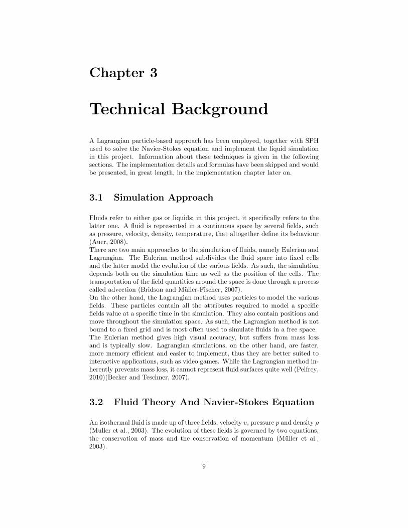
A Lagrangian particle-based approach has been employed, together with SPHused to solve the Navier-Stokes equation and implement the liquid simulationin this project. Information about these techniques is given in the followingsections. The implementation details and formulas have been skipped and wouldbe presented, in great length, in the implementation chapter later on.

3.1 Simulation Approach

Fluids refer to either gas or liquids; in this project, it specifically refers to thelatter one. A fluid is represented in a continuous space by several fields, suchas pressure, velocity, density, temperature, that altogether define its behaviour(Auer, 2008).There are two main approaches to the simulation of fluids, namely Eulerian andLagrangian. The Eulerian method subdivides the fluid space into fixed cellsand the latter model the evolution of the various fields. As such, the simulationdepends both on the simulation time as well as the position of the cells. Thetransportation of the field quantities around the space is done through a processcalled advection (Bridson and Muller-Fischer, 2007).On the other hand, the Lagrangian method uses particles to model the variousfields. These particles contain all the attributes required to model a specificfields value at a specific time in the simulation. They also contain positions andmove throughout the simulation space. As such, the Lagrangian method is notbound to a fixed grid and is most often used to simulate fluids in a free space.The Eulerian method gives high visual accuracy, but suffers from mass lossand is typically slow. Lagrangian simulations, on the other hand, are faster,more memory efficient and easier to implement, thus they are better suited tointeractive applications, such as video games. While the Lagrangian method in-herently prevents mass loss, it cannot represent fluid surfaces quite well (Pelfrey,2010)(Becker and Teschner, 2007).

3.2 Fluid Theory And Navier-Stokes Equation

An isothermal fluid is made up of three fields, velocity v, pressure p and density ρ(Muller et al., 2003). The evolution of these fields is governed by two equations,the conservation of mass and the conservation of momentum (Muller et al.,2003).

9

∂ρ

∂t+∇ · (ρv) = 0 (3.1)

The Lagrangian method (3.1) consists of a constant number of particles, eachhaving a fixed mass; as such, the conservation of mass is inherent and the cor-responding equation can be omitted (Muller et al., 2003). The conservation ofmomentum is given the Navier-Stokes equation and is used to describe the move-ment and evolution of the fluid. The following is the Navier-Stokes equation forincompressible fluids:

ρ

(∂v

∂t+ v · ∇v

)= −∇p+ µ∇2v + ρg (3.2)

where g is an external force and µ is the viscosity coefficient.

The Lagrangian particles move with the fluid and carry the fluid’s attributes inspace. As such, the convective derivative, v· ∇v, which gives the advection inthe Eulerian method, can be replaced by the substantial derivative Dv

Dt (Horvathand Illes, 2007). The Lagrangian Navier-Stokes equation therefore becomes:

ρdv

dt= −∇p+ µ∇2v + ρg (3.3)

The Navier-Stokes equation is the application of Newton’s second law of motionfor fluids; as such, the three terms making up the equation compute internaland external forces on the fluid, and can be differentiated to get the accelerationa and the velocities of the particles. The mass m is replaced by the density ρhere, since the ”mass in a volume”, given by the density, is more applicable forfluids (Auer, 2008).

a =F

m(3.4)

a =

(−∇p+ µ∇2v + ρg

)ρ

(3.5)

The three terms contribute to the internal and external force acting on the fluid,which result in the acceleration and thus movement of the fluid particles.

The first term gives the pressure force

−∇p (3.6)

and this is what holds the fluid molecules together without it, the whole fluidcollapses onto the ground. The pressure force is created whenever there is a

10

pressure difference and it acts in the direction from high pressure to low pres-sure along the negative of the pressure gradient (Auer, 2008). The pressuredepends on the density of the fluid, with a higher concentration of mass in avolume, or a higher density, giving rise to an increased force (from Newton’ssecond law), and this increases the pressure (from the definition of pressure,pressure is force per area). As such, the pressure term aims to equalise thedensity differences throughout the fluid (Pelfrey, 2010).

The second term gives the viscosity force

µ∇2v (3.7)

and this provides the resistance to the flow of particles, hence it defines howviscous the liquid is, such as in the case of water against honey. The Laplacianof the velocity field, ∇2v, gives the divergence of the latter from its averagevalue and thus, this force aims to restore or smooth this velocity difference.The viscosity coefficient µ defines how strongly the force acts.

The last term

ρg (3.8)

encompasses the external forces external, such as gravity or some wind or a user-generated interaction or surface tension, and will be discussed in more detailsin a later section.

3.3 Smoothed-Particle Hydrodynamics

The Lagrangian particles are finite in nature and are not enough to representthe continuous field of a fluid. SPH is an interpolation method that uses theseparticles as discrete samples to evaluate the state of the field at any positionwithin the fluid space; each particle is thought of as occupying a fraction of theproblem space (Kelager, 2006). The interpolation is done through the use ofradial symmetrical smoothing kernels, such that the approximation of a quantityA at some particle position r is given as a weighted sum of contributions fromneighbouring particles (Muller et al., 2003) as follows:

A(r) =∑j

mjAjρjW (r − rj , h) (3.9)

The distance h is the core radius and determines the amount of particles thatcontributes to the approximation value at position r. Beyond the distance h,

11

other particles have no effect on the calculation.

The SPH fluid equations also require the calculation of derivatives of the quan-tities. These affect only the smoothing kernel function, as follows:

∇A(r) =∑j

mjAjρj∇W (r − rj , h) (3.10)

∇2A(r) =∑j

mjAjρj∇2W (r − rj , h) (3.11)

The pressure and viscosity forces of the Navier-Stokes equation, described inthe previous section, can be easily calculated using SPH. However, these resultin non symmetric forces that would introduce instabilities in the simulation.Various alternatives have been developed and this will be discussed in details inthe implementation chapter later on.

Although SPH is very easy to understand and calculate, it was originally de-signed for compressible fluids and as such has to be carefully controlled to givevisually pleasing simulation of liquids. The compressibility issue is still an activeresearch topic for SPH.

3.4 Smoothing Kernel

The stability and accuracy of SPH calculations depend highly on the smoothingkernels. Moreover, since these calculations are done every single step of thesimulation, they directly influence the speed of the simulation. Muller et al.,2003, proposed the following three kernels:

• Poly6 KernelThis is the fastest kernel to compute, since r appears only squared, and isused in most of the calculations (Auer, 2008).

Wpoly6(r, h) =

{315

64πh9 (h2 − r2)3 , 0 ≤ r ≤ h0 , otherwise

(3.12)

with r = ||r||

∇Wpoly6(r, h) = −r945

32πh9(h2 − r2)2 (3.13)

12

∇2Wpoly6(r, h) = − 945

32πh9(h2 − r2)(3h2 − 7r2) (3.14)

• Spiky KernelThis gradient of this kernel is used instead for the pressure calculationbecause the gradient of the Poly6 kernel goes to zero near the centre; thiswould cancel any repulsive force between particles that get too close toeach other and thus would cause them to clump together (Auer, 2008).

∇Wspiky(r, h) = − 45

πh6r

||r||(h− r)2 (3.15)

• Viscosity KernelThe Laplacian of the Poly6 kernel also give negative values that wouldresult in high-energy viscosity forces and cause high-speed particles toaccelerate instead of slowing down. The viscosity kernel is used instead;it always gives a positive Laplacian to make the viscosity force act as adamping force in all cases and help reduce the velocity of high-energyparticles (Kelager, 2006).

∇2Wpoly6(r, h) =45

πh6(h− r) (3.16)

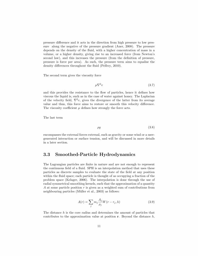
The following figure gives a visualisation of the three kernels:

Figure 3.1: Kernels used in the SPH method. (Red) Kernel value (Green)Gradient of kernel (Blue) Laplacian of kernel. Note that the kernels and theindividual curves are scaled differently in these plots. (Angst, 2007)

13

Chapter 4

Design

This chapter discusses all the design considerations required for the implementa-tion of the fluid simulation. These will form the basis of the final implementationand will influence the functionalities implemented by the end of the project.

4.1 Functional Requirements/Objectives

The aim of this project is to implement a 3D Lagrangian fluid solver using SPHto simulate the flow of liquids. The simulation will be based on the forces of theNavier-Stokes equation discussed in the previous chapter, with some additionalforces added to it. The following are some requirements of the solver:

• Simulation of the flow of liquids such as water, honey and etc.

• User interface to tweak the simulation parameters interactively.

• Interaction with boundary containers, such as boxes, and rigid bodies,such as spheres and mixers.

• Injection of particles, through a hose, to simulate effects such as a waterjet, rain, and etc.

• Simulation of the interaction of multiple fluids.

• Real-time visualisation of fluids using particles.

• Export of simulation data to an external application, such as Houdini, foradvanced rendering.

These objectives and functionalities will be adapted and updated throughoutthe implementation.

4.2 Entity Relationship Diagram

The following diagram shows the software architecture and the various classesthat make up the solution and the relationship linking them together. These re-lationships are directly reflected in the implementation of the software, throughclass inheritance and instantiation.

The following classes form the backbone of the software:

14

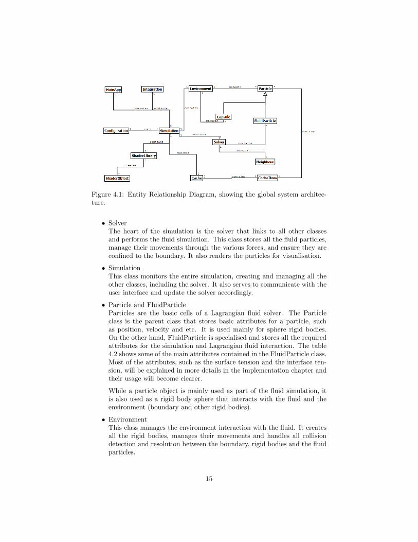
Figure 4.1: Entity Relationship Diagram, showing the global system architec-ture.

• SolverThe heart of the simulation is the solver that links to all other classesand performs the fluid simulation. This class stores all the fluid particles,manage their movements through the various forces, and ensure they areconfined to the boundary. It also renders the particles for visualisation.

• SimulationThis class monitors the entire simulation, creating and managing all theother classes, including the solver. It also serves to communicate with theuser interface and update the solver accordingly.

• Particle and FluidParticleParticles are the basic cells of a Lagrangian fluid solver. The Particleclass is the parent class that stores basic attributes for a particle, suchas position, velocity and etc. It is used mainly for sphere rigid bodies.On the other hand, FluidParticle is specialised and stores all the requiredattributes for the simulation and Lagrangian fluid interaction. The table4.2 shows some of the main attributes contained in the FluidParticle class.Most of the attributes, such as the surface tension and the interface ten-sion, will be explained in more details in the implementation chapter andtheir usage will become clearer.

While a particle object is mainly used as part of the fluid simulation, itis also used as a rigid body sphere that interacts with the fluid and theenvironment (boundary and other rigid bodies).

• EnvironmentThis class manages the environment interaction with the fluid. It createsall the rigid bodies, manages their movements and handles all collisiondetection and resolution between the boundary, rigid bodies and the fluidparticles.

15

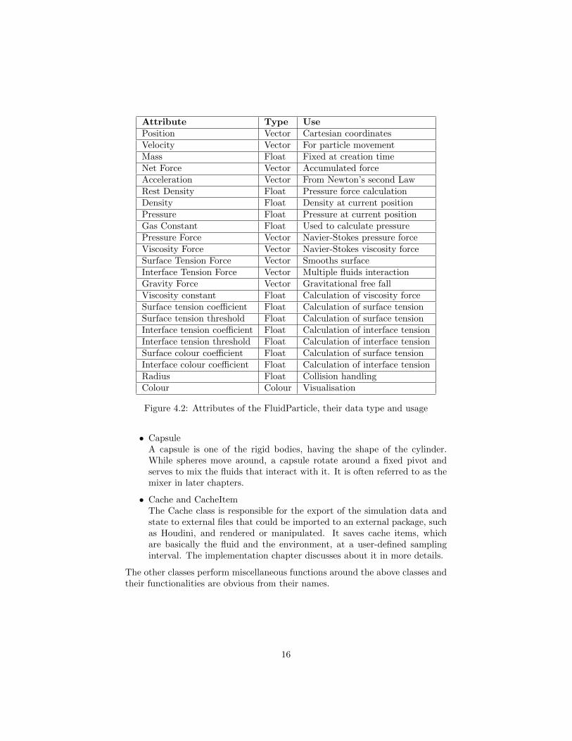
Attribute Type UsePosition Vector Cartesian coordinatesVelocity Vector For particle movementMass Float Fixed at creation timeNet Force Vector Accumulated forceAcceleration Vector From Newton’s second LawRest Density Float Pressure force calculationDensity Float Density at current positionPressure Float Pressure at current positionGas Constant Float Used to calculate pressurePressure Force Vector Navier-Stokes pressure forceViscosity Force Vector Navier-Stokes viscosity forceSurface Tension Force Vector Smooths surfaceInterface Tension Force Vector Multiple fluids interactionGravity Force Vector Gravitational free fallViscosity constant Float Calculation of viscosity forceSurface tension coefficient Float Calculation of surface tensionSurface tension threshold Float Calculation of surface tensionInterface tension coefficient Float Calculation of interface tensionInterface tension threshold Float Calculation of interface tensionSurface colour coefficient Float Calculation of surface tensionInterface colour coefficient Float Calculation of interface tensionRadius Float Collision handlingColour Colour Visualisation

Figure 4.2: Attributes of the FluidParticle, their data type and usage

• CapsuleA capsule is one of the rigid bodies, having the shape of the cylinder.While spheres move around, a capsule rotate around a fixed pivot andserves to mix the fluids that interact with it. It is often referred to as themixer in later chapters.

• Cache and CacheItemThe Cache class is responsible for the export of the simulation data andstate to external files that could be imported to an external package, suchas Houdini, and rendered or manipulated. It saves cache items, whichare basically the fluid and the environment, at a user-defined samplinginterval. The implementation chapter discusses about it in more details.

The other classes perform miscellaneous functions around the above classes andtheir functionalities are obvious from their names.

16

4.3 Simulation Pipeline

A fluid contains thousands of particles and layering and calculating their initialpositions manually for the simulation is too daunting and complicated a task.Steele et al. (2004) and Priscott (2010) discuss the use of external models andusing their vertices as initial positions for the particles.Using this method makes it very easy to create fluids of various shapes andresolutions, such as spheres and cubes, or even real-life models such as a houseor a creature, in an external package such as Maya or Houdini. These can thenbe exported to a standard obj format and loaded in the simulation engine.The simulation would primarily be visualised using particles, either OpenGLpoints or sphere primitives. While this serves as an interactive pre-visualisation,advanced rendering is more desired. Since this is not part of the scope of thisproject, functionality will be implemented to export the simulation data toan external format such as obj, which could then be easily rendered using anexternal application such as Maya or Houdini.

17

Chapter 5

Implementation

5.1 Simulation Algorithm

A basic simulation step typically calculates the density, pressure, then the var-ious forces such as pressure, viscosity, surface tension, interface tension andgravity. The acceleration is then integrated to get the next velocity and posi-tion. This is finally followed by collision detection and resolution, before theparticle is displaced.

Algorithm 1: Algorithm to perform simulation of fluid

Load and create fluid particlesInitialise neighbour search structure

while timer ticks doRefresh neighbour search structure

foreach particle P in particle list doL← Get neighbours of Pρ← Calculate density of P by iterating through Lp← Calculate pressure of P

end

foreach particle P in particle list doL← Get neighbours of PF pressure ← Calculate pressure force for P by iterating through LF viscosity ← Calculate viscosity force for P by iterating through L

F surface ← Calculate surface tension force for P by iterating through L

F interface ← Calculate interface tension force for P by iteratingthrough LF gravity ← Calculate gravitational force on P

Fnet = F pressure + F viscosity + F surface + F interface + F gravity

a = F/ρIntegrate a to get velocity v and position xApply collision detection and resolution on P against environmentMove P and render it

end

end

18

5.2 Fluid Creation

As mentioned in the design chapter, the fluid is created from an external modelthat imported from a file. Model creation has been done in Houdini usingprimitives such as poly sphere or poly box. Since this is not enough to providethe required number of vertices for a proper simulation, the pointsfromvolumesop has been used to fill the primitives with points/vertices. The parameter tabeven allow specifying the number of points, thus the number of particles thatform the simulation eventually can be easily controlled, and thus its resolution.

Figure 5.1: Fluid model creation in Houdini

The final model is exported to an obj file and loaded using the NGL graphicslibrary (Macey, 2010). The mass of the particles is fixed at creation time andcalculated as follows (Kelager, 2006):

mass = density ∗ volume

particlecount(5.1)

Algorithm 2: Algorithm for creation of the fluid particles

Load modelRead rest density ρ0 and volume V from configuration fileGet vertex count n from modelCalculate mass m = ρ0 ∗ V/nforeach vertex v do

Create particle, with mass = m, position = vAdd particle to solver particle list

end

19

5.3 Force Calculation

This section describes in details the implementation of the various forces, whichis the essential part of the fluid solver and that uses SPH as its base. Thepressure and viscosity forces, which are directly obtained from the Navier-Stokesequations, have been discussed briefly in the Technical Background chapter.Apart from these two basic forces, two additional forces, surface tension andinterface tension, are also discussed. This section also makes constant referenceto the three smoothing kernels that were discussed in the Technical Backgroundchapter.

5.3.1 Pressure and Density

The density, and consequently, the pressure must be evaluated at every particle’sposition as it evolves throughout the simulation. The pressure is computed usinga modified version of the ideal gas state equation that was proposed by Desbrunand Cani (1996) and used by Muller et al. (2003), as follows:

p = k(ρ− ρ0) (5.2)

where ρ0 is the rest density of the fluid and k is the gas constant.

This equation introduces a spring-like behaviour to the pressure calculation;while a density higher than the rest value produces a positive pressure thatpushes the particles away, a lower density will result in a negative pressure andbrings the particles together. The gas constant k depends on the temperatureof the fluid and determines how strongly the pressure difference in the fluid isequalised.

The density at position r is calculated using SPH, as follows (Kelager, 2006):

ρi =∑j

ρjmj

ρjW (ri − rj , h)

=∑j

mjW (ri − rj , h) (5.3)

Once, the pressure and density is computed, the pressure force is calculated byusing SPH and the Poly6 smoothing kernel (3.12) (3.13) (3.14). The followingequation resolves the non-symmetrical force issue (Kelager, 2006) and is usedin this project:

20

fpressurei = −ρi∑j 6=i

(piρ2i

+pjρ2j

)mj∇W (ri − rj , h) (5.4)

Since the pressure and density must be found for all particles prior to the cal-culations of the forces, two loops must be used as shown in the simulationalgorithm in the previous section; one to calculate the pressures and densities,then the other to calculate the actual forces.

5.3.2 Viscosity

The viscosity force acts not only as a damping force to particles, but also pro-vides stability to the simulation. As mentioned earlier, only using SPH givesrise to a non-symmetric force; Muller et al. (2003) proposes the use of velocitydifference instead of absolute values to solve this issue as follows:

fviscosityi = µ∑j 6=i

(vj − vi)mj

ρj∇2W (ri − rj , h) (5.5)

where v is the velocity of the particles.

5.3.3 Surface Tension

The surface tension force is an external force that is not from the Navier-Stokesequation and acts only on particles at the surface of the fluid. Its implementa-tion is discussed in more details in this section.

Molecules inside a fluid are held in perfect balance through intermolecular at-traction that is equal in all directions. However, this is not the case for particlesat the surface of the fluid and this imbalance gives rise to the surface tensionforce. The latter acts along the surface normal in an inward direction towardsthe fluid and aims to reduce the curvature of the surface and thus, smooths thefluid surface (Muller et al., 2003).

The following formulas have been adapted from the paper of Kelager (2006).Acolour field c is used to identify the surface of the fluid. Each particle is given acolour quantity of 1, while air is given a value of 0. It is calculated using SPHas follows:

21

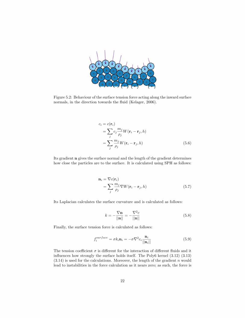
Figure 5.2: Behaviour of the surface tension force acting along the inward surfacenormals, in the direction towards the fluid (Kelager, 2006).

ci = c(ri)

=∑j

cjmj

ρjW (ri − rj , h)

=∑j

mj

ρjW (ri − rj , h) (5.6)

Its gradient n gives the surface normal and the length of the gradient determineshow close the particles are to the surface. It is calculated using SPH as follows:

ni = ∇c(ri)

=∑j

mj

ρj∇W (ri − rj , h) (5.7)

Its Laplacian calculates the surface curvature and is calculated as follows:

k = − ∇n

||n||= −∇

2c

||n||(5.8)

Finally, the surface tension force is calculated as follows:

fsurfacei = σkini = −σ∇2cini||ni||

(5.9)

The tension coefficient σ is different for the interaction of different fluids and itinfluences how strongly the surface holds itself. The Poly6 kernel (3.12) (3.13)(3.14) is used for the calculations. Moreover, the length of the gradient n wouldlead to instabilities in the force calculation as it nears zero; as such, the force is

22

only calculated when the gradient length exceeds a threshold value β, else it istaken as zero (Kelager, 2006).

Algorithm 3: Algorithm for the calculation of the surface tension force

foreach particle P in particle list dogradient← vector(0)laplacian← 0L← Get neighbours of P

foreach neighbour N in neighbour list L dom← mass of Nρ← density of Ngradient← gradient+ ((m/ρ) ∗Wpoly6gradient

laplacian← laplacian+ ((m/ρ) ∗Wpoly6laplacian

endif length(gradient) > β then

F surface ← −σ ∗ normalise(gradient) ∗ laplacianendelse

F surface ← 0end

end

5.3.4 Interface Tension

The interface tension force is another additional external force that was firstsuggested by Muller et al. (2005) for the interaction of multiple fluids. Theinterface force acts perpendicular to the interface between the two fluids tominimise its curvature.It is an adaptation of the surface tension force, discussed in the previous section,with the only difference being the colour field. Here, the interaction of polarand non-polar fluids is considered. Polar fluids tend to mix with polar fluidsand are given a colour value −0.5; on the other hand, a polar fluid doesn’t mixwith a non-polar one and the latter bear a colour value of +0.5 (Muller et al.,2005).The calculation of the gradient and Laplacian is similar to that for the surfacetension, except that it uses the new colour values 0.5 and −0.5.

5.3.5 Gravity

The gravitational force is yet another external force that is caused by the accel-eration due to gravity, called free fall, and it acts in the negative y direction. Ithas a value of (0,−9.8, 0). Other external forces follow suit and can be imple-mented by a simple vector. For example, the addition of a vector (5, 0, 0) to the

23

accumulation of forces could be interpreted as a wind blowing in the positive xdirection.

5.4 Integration

The acceleration of the particles is computed by dividing the net force, discussedin the previous section, by their density. The next step is to integrate the ac-celeration to find the new velocity and position of the particle. Two integrationmethods have been implemented in this project, namely, semi-implicit Eulerand leap-frog.

5.4.1 Semi-Implicit Euler

While the explicit Euler method is the simplest integration method, it suf-fers from serious instabilities if the integration time-step is kept large. Thesemi-implicit Euler method, which is a slight derivative of the explicit Euler, isimplemented in this project. The latter also suffers from numerical instabilitieswith big time-steps; however, it is known to conserve energy and thus is slightlymore accurate. It is calculated as follows:

vi+1 = vi + a · dt (5.10)

xi+1 = xi + vi+1 · dt (5.11)

5.4.2 Leapfrog

The Leapfrog integration is a second order method that is more accurate thanthe first-order Euler method. It calculates velocities and positions at interleavedtimes, with the velocities calculated at half times and the positions calculated atfull integer times. The velocity and position are calculated as follows (Priscott,2010):

vi+1/2 = vi−1/2 + a · dt (5.12)

xi+1 = xi + vi+1/t · dt (5.13)

The initial velocity offset v−1/2 is calculated using the Euler method as follows:

v−1/2 = v0 −1

2· dt · a0 (5.14)

24

In this project, the leap-frog method has been implemented using a different setof formulas (Hut and Makino, 2004), which are similar to the previous formulasbut have been rearranged and rewritten to calculate the velocity and positionat full time steps. The derived formulas are as follows:

vi+1 = vi +(ai + ai+1) · dt

2(5.15)

xi+1 = xi + vi · dt+ai · dt2

2(5.16)

The velocity is calculated from the average of the current acceleration and nextacceleration, therefore providing more stability to the next displacement of theparticles.

5.5 Neighbour Search and Spatial Hashing

The search of neighbours and their contributions is a vital part of SPH; it is per-formed at every time-step of the simulation and directly impacts the accuracyof the SPH calculations as well as the speed of the simulation. A naive approachof checking every particle against all other particles results in a complexity ofO(n2). This is most undesirable since it limits the number of particles that canbe simulated. Also, the smoothing kernels of SPH use a core radius h beyondwhich, all other particles have no contribution to the current particle and search-ing them results in a waste of CPU resource. Several algorithms exist to findneighbours efficiently and fall under the Nearest Neighbour Search algorithms.One such very efficient algorithm which is suited to SPH fluid simulation is spa-tial hashing, developed by Teschner et al. (2003); this algorithm decreases thecomplexity from O(n2) to O(nm), with m being the average number of num-bers found and this can even be reduced with a more uniform distribution ofparticles (Kelager, 2006).

Spatial Hash FunctionThe spatial hashing method uses a hash function that converts a 3D position inspace to a scalar hash key. This key is then used as an index to a hash-map tostore particles in cells, as well as to retrieve neighbouring particles.

The hash function is the heart of this method, and it has been designed toprevent the particles that are significantly apart to be hashed to the same cell(Priscott, 2010). Kelager (2006) defines it as follows:

hash(r) = (rxp1 xor ryp2 xor ryp3) mod nH (5.17)

25

A discretising function is used (Kelager, 2006) that divides the position by thecell size l, and returns the rounded integer values, as follows:

r(r) = (brx/lc, bry/lc, brz/lc)T (5.18)

The cell size l is the smoothing length used in our SPH kernel calculations.

nH is the hash map size and is calculated as follows:

nH = prime(2n) (5.19)

Where n is the particle count and the function prime(x) gives the next primenumber ≥ x.

The last missing piece to the hash function equation is the values of p1, p2 andp3. These are large prime numbers and are suggested by Kelager (2006) asfollows:

p1 = 73856093, p2 = 19349663, p3 = 83492791 (5.20)

Insertion in Hash MapNow that the hash function is defined, the insertion of the particles and thefilling in of the hash map is to be done. This is executed before the calculationof the forces.

Algorithm 4: Algorithm for the insertion of particles in the hash map

Clear hash mapforeach particle P in particle list do

x← Get position Px← discretise(x)hashKey ← hashFunction(x)Insert < hashKey, P > in hash map

end

Searching of NeighboursOnce the hash map is refreshed, the neighbours of a particle can be searched byfirst generating the hash key from its position, then retrieving all particles fromthe map with the generated hash key as an index. This, however, is not enoughsince not all neighbouring particles are hashed to the same cell. Kelager (2006)also suggests the use of a bounding box, so that the search area is extended

26

around the particle. The bounding box limits for a particle at position r aredefined as follows:

BBmin = r(r− (h, h, h)T ) , BBmax = r(r + (h, h, h)T ) (5.21)

A bounding box is used since it is very easy to calculate its limits and iteratethrough it; however, only particles within the distance of the smoothing lengthfrom the searched position is required, as follows:

||r− rj || ≤ h (5.22)

Algorithm 5: Algorithm used to find the neighbours for a particle (adaptedfrom Priscott (2010))

Input: A particle P with position X

1. get particles in the same cell as particle PGenerate hash key key using position XGet all particles in the map with the generated hash key keyAdd to neighbour list

2. define bounding box and search particles within thatDefine bounding box limits BBMin and BBMaxDiscretise BBMin and BBMaxfor BBMin to BBMax do

Create a Cartesian position c within the bounding boxGenerate hash key key2 for the created position cSearch for particles from the map having the generated hash key key2if they are not duplicates then

if they are within smoothing distance h thenthen add them to neighbour list

end

end

end

5.6 Environment Interaction

The environment consists of the boundary and rigid bodies. These interact withthe fluid particles and modify their behaviour. Kelager (2006) suggested the useof implicit functions to model rigid bodies such as spheres and capsules and thishas been implemented in this project. While an implicit function doesn’t givesimply control over the shapes of the rigid bodies, it helps keep the computationsless complex because implicit surfaces can be defined very easily with few singlemathematical functions. The collision handling mechanism, implemented in

27

this project, assumes that the environment is fixed such that the fluid particlesdo not influence them; while this is not true in real-life and violates Newton’sthird law of motion of action-reaction, it keeps the collision handling easier andless-computationally intensive.

5.6.1 Collision Detection and Handling

Collision detection is performed at every time-step for all the particles. It sim-ply involves solving the implicit function at the current position of the particles;a negative result from the function, F (x) < 0 implies that collision has occurred.

Once collision is detected, the following needs to be determined for the resolu-tion, as follows:

• the contact point cp where the particle penetrate the obstacle’s surface,

• the penetration depth d that is given by the value of the solved implicitfunction, and

• the surface normal n of the collided surface.

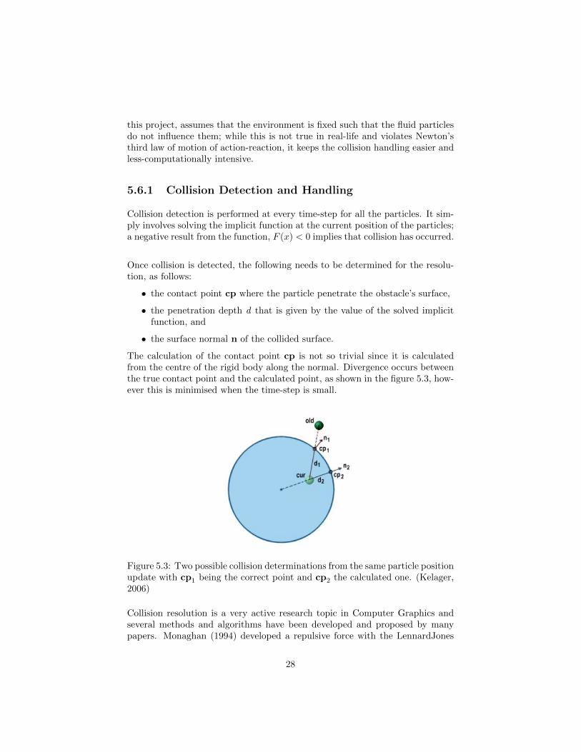
The calculation of the contact point cp is not so trivial since it is calculatedfrom the centre of the rigid body along the normal. Divergence occurs betweenthe true contact point and the calculated point, as shown in the figure 5.3, how-ever this is minimised when the time-step is small.

Figure 5.3: Two possible collision determinations from the same particle positionupdate with cp1 being the correct point and cp2 the calculated one. (Kelager,2006)

Collision resolution is a very active research topic in Computer Graphics andseveral methods and algorithms have been developed and proposed by manypapers. Monaghan (1994) developed a repulsive force with the LennardJones

28

potential, called boundary force. Bell et al. (2005) introduces penalty force-based to resolve collision. Impulse-based collision response is a very populartechnique that modifies the velocity of the particle at the time of collision. Inthis project, the hybrid impulse-projection method proposed by Kelager (2006)is used, which simply projects the collided particle back to the surface along thesurface normal.

This new position ri, in the case of our implicit surfaces, is simply the contactpoint:

ri = cp (5.23)

The velocity is reflected back along the surface normal. A restitution coefficient,cR such that 0 ≤ cR ≤ 1, is used to determine the amount of the velocityreflected back, thus mimicking the loss of energy during a collision, with a valueof 0 giving rise to an inelastic collision and a value of 1 simulating a perfectlyelastic situation (Kelager, 2006). The formula to calculate the velocity is asfollows:

vi = vi − (1 + cR)(vi · n)n (5.24)

5.6.2 Environment Objects

5.6.2.1 Boundary

The boundary is implemented using a primitive bounding box. This is the sim-plest primitive and allows for really cheap calculations to detect and resolvecollision.

The box is defined as a collection of 6 faces, each representing a limit XMin,XMax, YMin, YMax, ZMin and ZMax. The x, y and z components of the par-ticle’s position is simply checked against these limits. In case of collision, theyare set to these limit values.

The new velocity follows the same line as the formula discussed in the previoussection. However, since the latter involves dot product and vector multiplica-tion, it is a bit costly. In the case of a bounding box, the surface normals arethe unit normals. Thus, the velocity is simply reflected as follows:

vi = vi ∗ −cR (5.25)

29

5.6.2.2 Periodic Wall Boundary

A periodic wall is also implemented in this project. This is an extension ofthe boundary box, discussed in the previous section and as such, has the samecollision handling mechanism.

A periodic sine function is used to move the right wall, found at the maximumx direction, up to a maximum amplitude of a to and from its initial position p0.

a sin(bθ) (5.26)

Increasing the value of a will make the wall have larger displacements around itsrest position. The angle θ of the sine function can also be multiplied by a scalefactor b to increase or decrease the period of the function and thus, influencethe speed of the wall movement.

Figure 5.4: sine wave with amplitude a and b = 1. Adapted from http:

//commons.wikimedia.org/wiki/Image:Sine.svg

5.6.2.3 Rigid Bodies

As mentioned initially, the rigid bodies are modelled with implicit functions,which are easy to define and allow simple collision detection mechanism. Tworigid bodies have been implemented in this project, a sphere and a capsule.

SphereA sphere is the simplest implicit surface to define, using the following formula(Kelager, 2006):

Fsphere(x) = ||x− c||2 − r2 (5.27)

where c is the centre of the sphere and r its radius.

The contact point cp is calculated as follows:

30

cpsphere = c + rx− c

||x− c||(5.28)

The penetration depth d is given by:

dsphere = |||c− x|| − r| (5.29)

where |a| gives the absolute value of a.

The unit surface normal n is calculated using the following formula:

nsphere = sgn(Fsphere(x))c− x||c− x||

(5.30)

Spheres are free to move and interact with the fluids, boundary, capsules andother spheres. They are also subject to gravitational forces and act as a fullrigid body within the container.

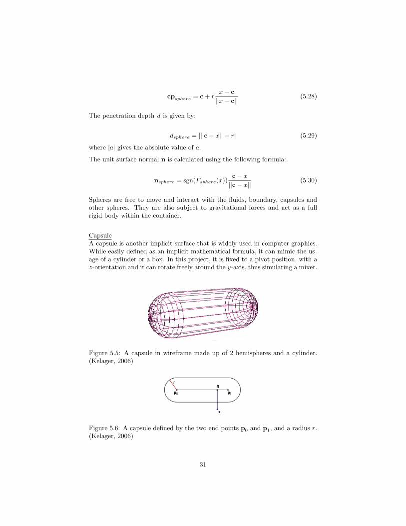
CapsuleA capsule is another implicit surface that is widely used in computer graphics.While easily defined as an implicit mathematical formula, it can mimic the us-age of a cylinder or a box. In this project, it is fixed to a pivot position, with az -orientation and it can rotate freely around the y-axis, thus simulating a mixer.

Figure 5.5: A capsule in wireframe made up of 2 hemispheres and a cylinder.(Kelager, 2006)

Figure 5.6: A capsule defined by the two end points p0 and p1, and a radius r.(Kelager, 2006)

31

A capsule is defined using the following formula:

Fcapsule(x) = ||q− x|| − r (5.31)

where

q = p0 +

(min

(1,max

(0,− (p0 − x) · (p1 − p0)

||p1 − p0||2

)))(p1 − p0) (5.32)

The contact point cp is calculated as follows:

cpcapsule = q + rx− q

||x− q||(5.33)

The penetration depth d is given by:

dcapsule = |Fcapsule(x)| (5.34)

The unit surface normal n is calculated as follows:

ncapsule = sgn(Fcapsule(x))q− x||q− x||

(5.35)

A sgn function is used in the calculation of the surface normals; this simplygives the sign of the function, positive or negative.

5.7 Particle Injection

Functionality was implemented to allow the injection of particles into the fluid.As with the fluid model, the injected particles also are loaded from an externalmodel and the latter typically has a reduced particle count. A list of particleprototypes is kept in a separate list; each one of those contains the basic prop-erties for the fluid that it represents. Therefore, if there are 2 fluids loaded in

32

the simulation, the list contains 2 prototypes.

Algorithm 6: Algorithm used to inject particles into the fluid simulation

Get index i of current fluid for which particles are to be injectedGet particle prototype p for the index iforeach injected model vertex v do

Create a particle Z with position = v and properties = pAdd Z to list of particles forming the fluid

end

This approach allows the new particles to be added to the same list of particlesthat make up the simulation fluid. Therefore, once these particles are injected,they no longer differ from the fluid particles and get subjected to the same SPHforces as all others.

There is an option that is provided to specify the time at which these particlesstart behaving like fluid particles; this could be as soon as they are injected, orwhen they hit the boundary or some rigid body. Varying this gives some veryinteresting effects. Screenshots have been given in the Simulation, Results andEvaluation chapter

5.8 Visualisation and Data Exporting

5.8.1 OpenGL Rendering

As stated initially, specialised rendering techniques, such as raycasting, is notpart of the scope of this project. The particles have been rendered as sphereprimitives, using OpenGL. Each fluid is given a specific colour so that theirinteractive can be observed. The obvious disadvantage of this approach is thatgaps appear in low-density regions. One approach, suggested by Kelager (2006)is to modify the radius of the sphere to increase or decrease according to thedensity and thus cover the gaps; this has not been implemented in this projectas additional calculations are required and visualisation is not the primary focusof this project.

5.8.2 Exporting Simulation Data To Houdini

The ability to export simulation data and state is implemented in this project,so that better and enhancement rendering can be achieved. The export is specif-ically done to geo files, which is Houdinis native geometry ASCII format. This

33

file format can be easily read and written to, thus the reason for choosing itfor this project. Moreover, being native to Houdini, it is very easy to load inHoudini and per-frame animation is very fast.

While the contents of the geo file could contain all sort of combination betweenvarious attributes, primitives, groups and etc., a simple approach to exportpoints has been adopted here. The latter is achieved by writing the set ofpoints as homogeneous x, y, z and w coordinates, one per line. Once exportedto a geo file, loading in Houdini is intuitive with the file sop. Point manipulationin Houdini is a very common task and lots of enhancements could be applied toparticles to render them in multiple forms.One very easy method is the use of the copy sop to copy spheres or otherprimitives onto the particles and thus have a simulation of spheres (Horvathand Illes, 2007). Houdini provides another very interesting sop called parti-clefromfluid which generates a surface from the simulation particles. Furtherenhancements can be done, such as the application of a procedural liquid shader.In brief, Houdini itself takes care of all the visualisation process; all it needs isthe simulation data and this has been implemented in this project.

Apart from the fluid particles, the positions of the rigid bodies can also beexported. The rigid bodies could thus be reconstructed in Houdini with en-hancements and behave according to the simulation data. The boundary boxtransformations are also exported, thus its periodic movements can be recreatedin Houdini.

34

Chapter 6

Simulation, Results and Eval-uation

This chapter focuses on the simulation, setup parameters and execution. Variousscenarios are discussed and simulated to show the usability and flexibility of thesimulation. The chapter ends on a discussion of some of the issues dealt withthe simulation and efficiency considerations of the implemented solution.

6.1 Simulation Parameters

While it is desired to have the parameters of the simulation set to true real-lifevalues, this is not always possible, either because the true values are too big forthe simulation, such as the gas constant or they are too tiny such as in the caseof the surface tension coefficient. Many of the parameters are left to the user fortweaking to achieve a stable simulation. Moreover, large viscosity and dampingis required to take care of the various pressure shocks that would otherwise ex-plode the simulation. Due to this, the range of viscosity values that could besimulated is really narrow. The mass of the particles has also to be set high sothat the heaviness stabilise the simulation.

6.2 Scenarios and Results

Various scenarios have been setup and simulated, that includes the interactionof multiple fluids with the different rigid bodies, spheres and capsules, arrangedin diverse ways. Some very interesting scene setups have been made and theresults obtained are demonstrated in the following sections.

6.2.1 Single Fluid

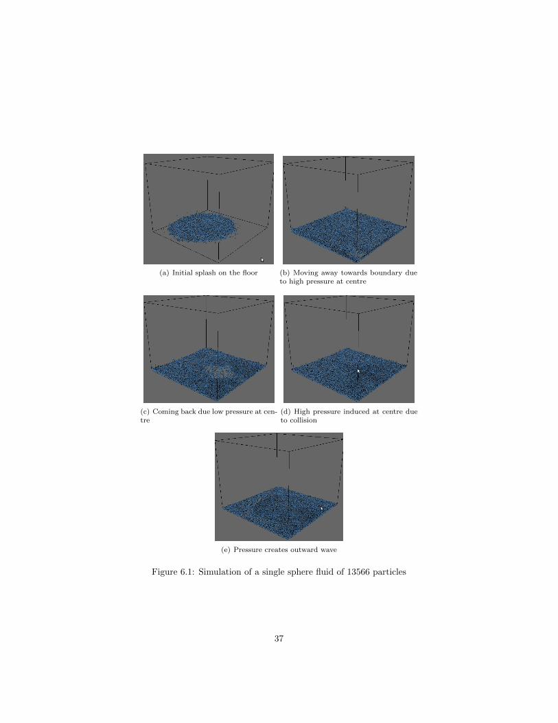
Several scenarios were simulated, figure 6.1 and figure 6.2 and in all of the cases,4 phases in the flow of the liquid flow were observed:

1. particles falling down and splashing on the floor,

35

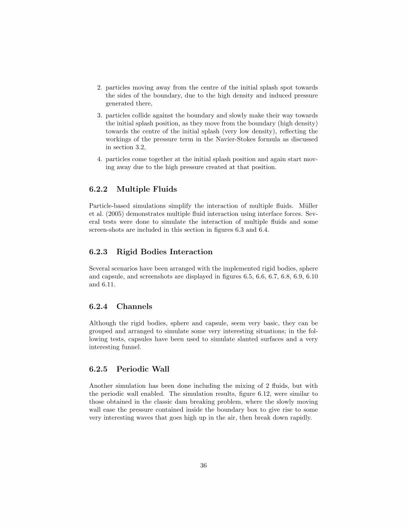
2. particles moving away from the centre of the initial splash spot towardsthe sides of the boundary, due to the high density and induced pressuregenerated there,

3. particles collide against the boundary and slowly make their way towardsthe initial splash position, as they move from the boundary (high density)towards the centre of the initial splash (very low density), reflecting theworkings of the pressure term in the Navier-Stokes formula as discussedin section 3.2,

4. particles come together at the initial splash position and again start mov-ing away due to the high pressure created at that position.

6.2.2 Multiple Fluids

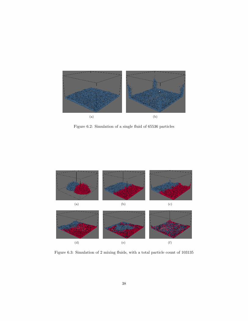
Particle-based simulations simplify the interaction of multiple fluids. Mulleret al. (2005) demonstrates multiple fluid interaction using interface forces. Sev-eral tests were done to simulate the interaction of multiple fluids and somescreen-shots are included in this section in figures 6.3 and 6.4.

6.2.3 Rigid Bodies Interaction

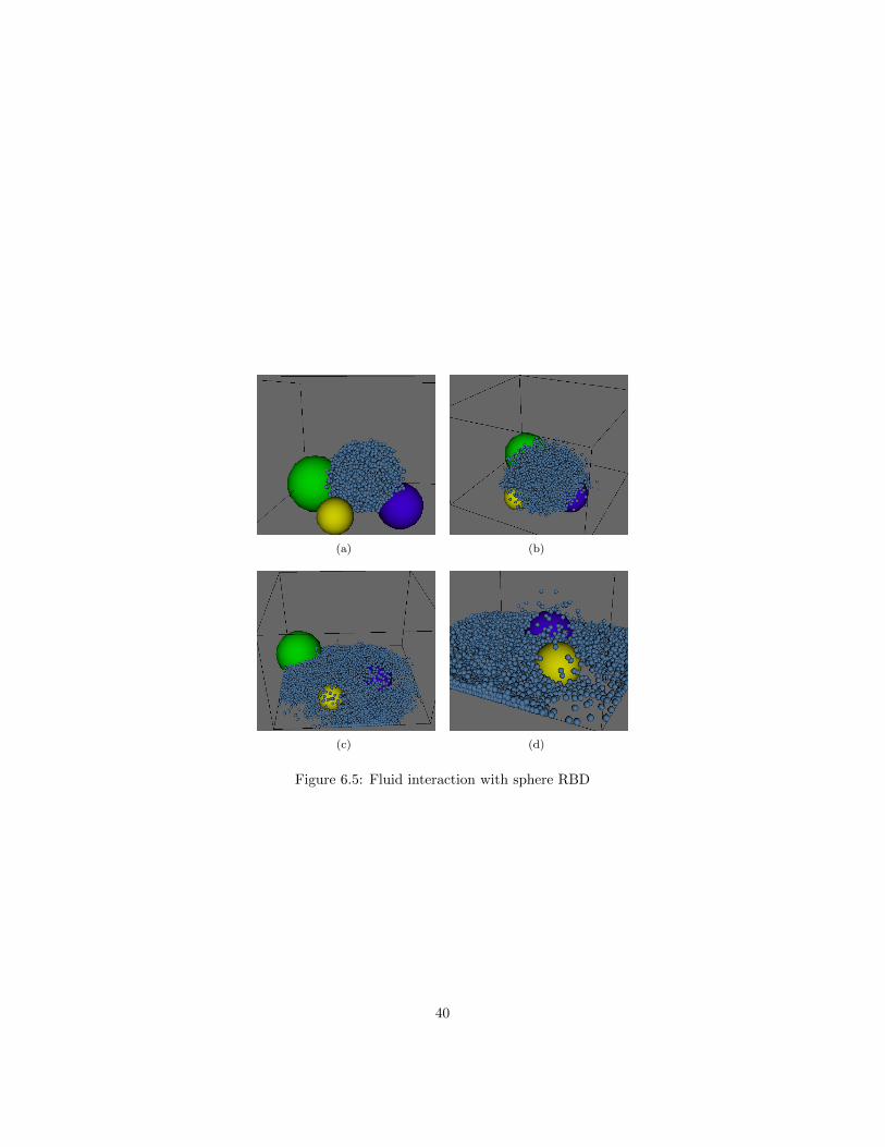
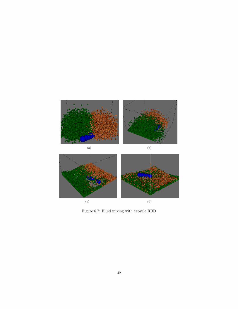
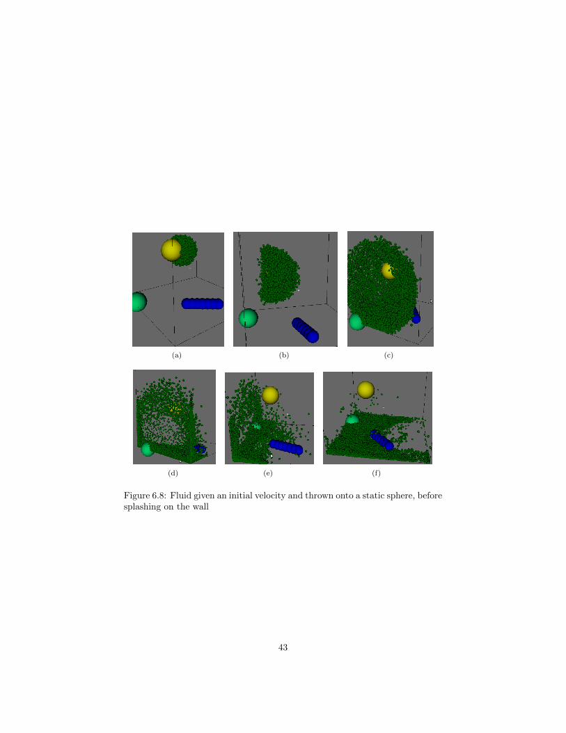
Several scenarios have been arranged with the implemented rigid bodies, sphereand capsule, and screenshots are displayed in figures 6.5, 6.6, 6.7, 6.8, 6.9, 6.10and 6.11.

6.2.4 Channels

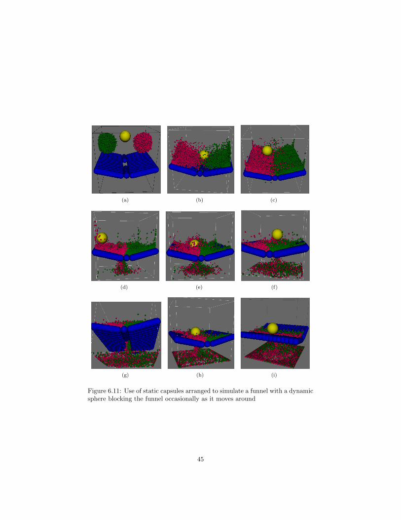
Although the rigid bodies, sphere and capsule, seem very basic, they can begrouped and arranged to simulate some very interesting situations; in the fol-lowing tests, capsules have been used to simulate slanted surfaces and a veryinteresting funnel.

6.2.5 Periodic Wall

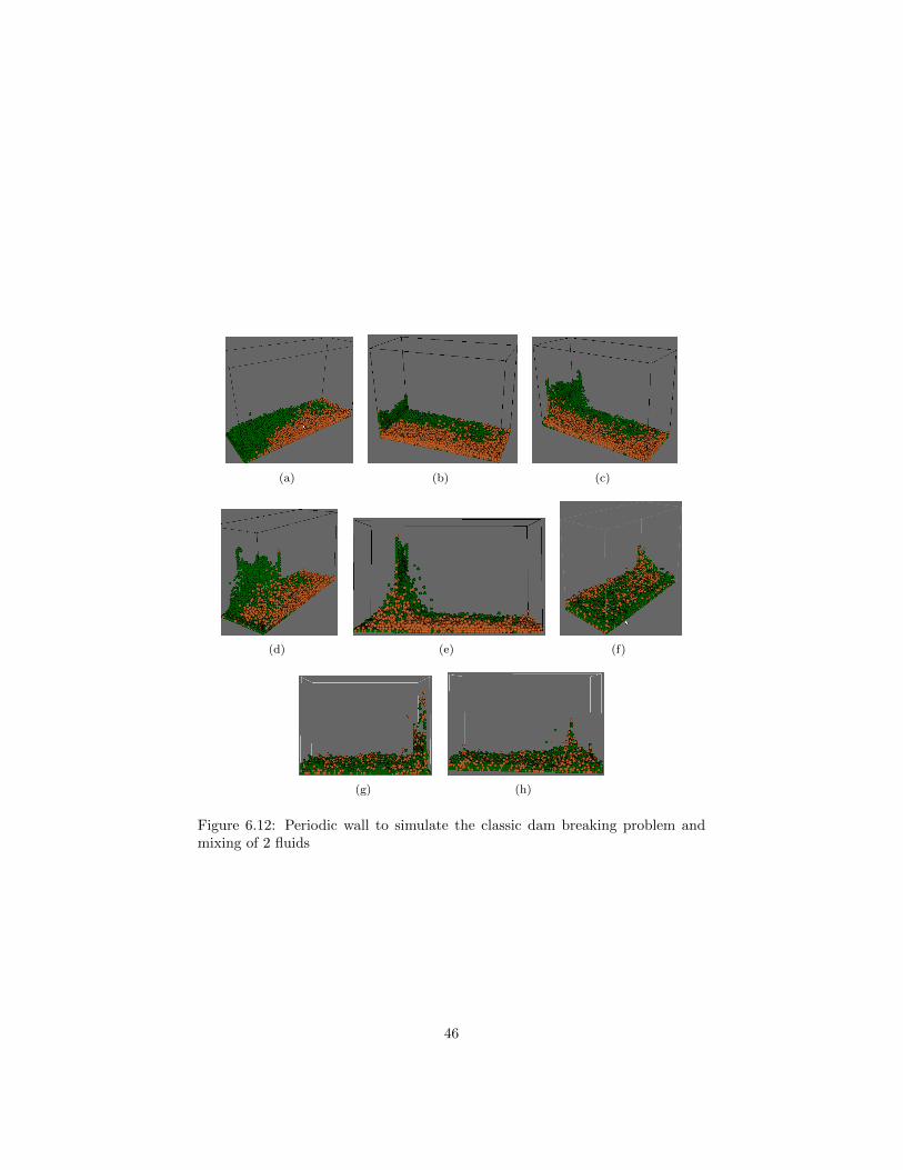
Another simulation has been done including the mixing of 2 fluids, but withthe periodic wall enabled. The simulation results, figure 6.12, were similar tothose obtained in the classic dam breaking problem, where the slowly movingwall ease the pressure contained inside the boundary box to give rise to somevery interesting waves that goes high up in the air, then break down rapidly.

36

(a) Initial splash on the floor (b) Moving away towards boundary dueto high pressure at centre

(c) Coming back due low pressure at cen-tre

(d) High pressure induced at centre dueto collision

(e) Pressure creates outward wave

Figure 6.1: Simulation of a single sphere fluid of 13566 particles

37

(a) (b)

Figure 6.2: Simulation of a single fluid of 65536 particles

(a) (b) (c)

(d) (e) (f)

Figure 6.3: Simulation of 2 mixing fluids, with a total particle count of 103135

38

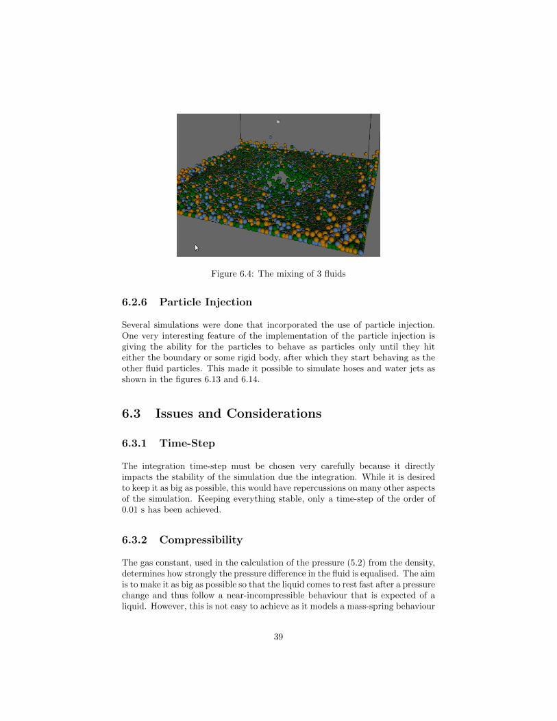
Figure 6.4: The mixing of 3 fluids

6.2.6 Particle Injection

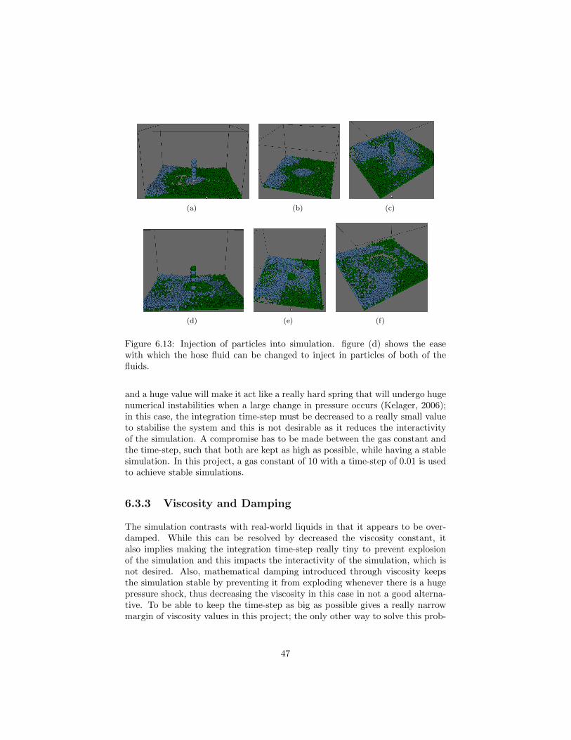
Several simulations were done that incorporated the use of particle injection.One very interesting feature of the implementation of the particle injection isgiving the ability for the particles to behave as particles only until they hiteither the boundary or some rigid body, after which they start behaving as theother fluid particles. This made it possible to simulate hoses and water jets asshown in the figures 6.13 and 6.14.

6.3 Issues and Considerations

6.3.1 Time-Step

The integration time-step must be chosen very carefully because it directlyimpacts the stability of the simulation due the integration. While it is desiredto keep it as big as possible, this would have repercussions on many other aspectsof the simulation. Keeping everything stable, only a time-step of the order of0.01 s has been achieved.

6.3.2 Compressibility

The gas constant, used in the calculation of the pressure (5.2) from the density,determines how strongly the pressure difference in the fluid is equalised. The aimis to make it as big as possible so that the liquid comes to rest fast after a pressurechange and thus follow a near-incompressible behaviour that is expected of aliquid. However, this is not easy to achieve as it models a mass-spring behaviour

39

(a) (b)

(c) (d)

Figure 6.5: Fluid interaction with sphere RBD

40

(a) (b)

(c) (d)

Figure 6.6: More fluid interaction with dynamic sphere RBD

41

(a) (b)

(c) (d)

Figure 6.7: Fluid mixing with capsule RBD

42

(a) (b) (c)

(d) (e) (f)

Figure 6.8: Fluid given an initial velocity and thrown onto a static sphere, beforesplashing on the wall

43

(a) (b)

(c) (d)

Figure 6.9: Dynamic Sphere simulating a bullet through the fluid

(a) (b) (c)

Figure 6.10: Static capsules arranged to simulate a slanted hard surface

44

(a) (b) (c)

(d) (e) (f)

(g) (h) (i)

Figure 6.11: Use of static capsules arranged to simulate a funnel with a dynamicsphere blocking the funnel occasionally as it moves around

45

(a) (b) (c)

(d) (e) (f)

(g) (h)

Figure 6.12: Periodic wall to simulate the classic dam breaking problem andmixing of 2 fluids

46

(a) (b) (c)

(d) (e) (f)

Figure 6.13: Injection of particles into simulation. figure (d) shows the easewith which the hose fluid can be changed to inject in particles of both of thefluids.

and a huge value will make it act like a really hard spring that will undergo hugenumerical instabilities when a large change in pressure occurs (Kelager, 2006);in this case, the integration time-step must be decreased to a really small valueto stabilise the system and this is not desirable as it reduces the interactivityof the simulation. A compromise has to be made between the gas constant andthe time-step, such that both are kept as high as possible, while having a stablesimulation. In this project, a gas constant of 10 with a time-step of 0.01 is usedto achieve stable simulations.

6.3.3 Viscosity and Damping

The simulation contrasts with real-world liquids in that it appears to be over-damped. While this can be resolved by decreased the viscosity constant, italso implies making the integration time-step really tiny to prevent explosionof the simulation and this impacts the interactivity of the simulation, which isnot desired. Also, mathematical damping introduced through viscosity keepsthe simulation stable by preventing it from exploding whenever there is a hugepressure shock, thus decreasing the viscosity in this case in not a good alterna-tive. To be able to keep the time-step as big as possible gives a really narrowmargin of viscosity values in this project; the only other way to solve this prob-

47

(a) (b)

(c) (d)

Figure 6.14: Directional injection of particles into simulation with interactionwith capsule mixer to simulate water jet and rain. The hose particle initiallybehave as particles only, until they first hit a rigid body, after which they startbehaving as fluid particles.

48

lem is using implicit integration, but this process is very computation-intensive.

6.3.4 Smoothing Length

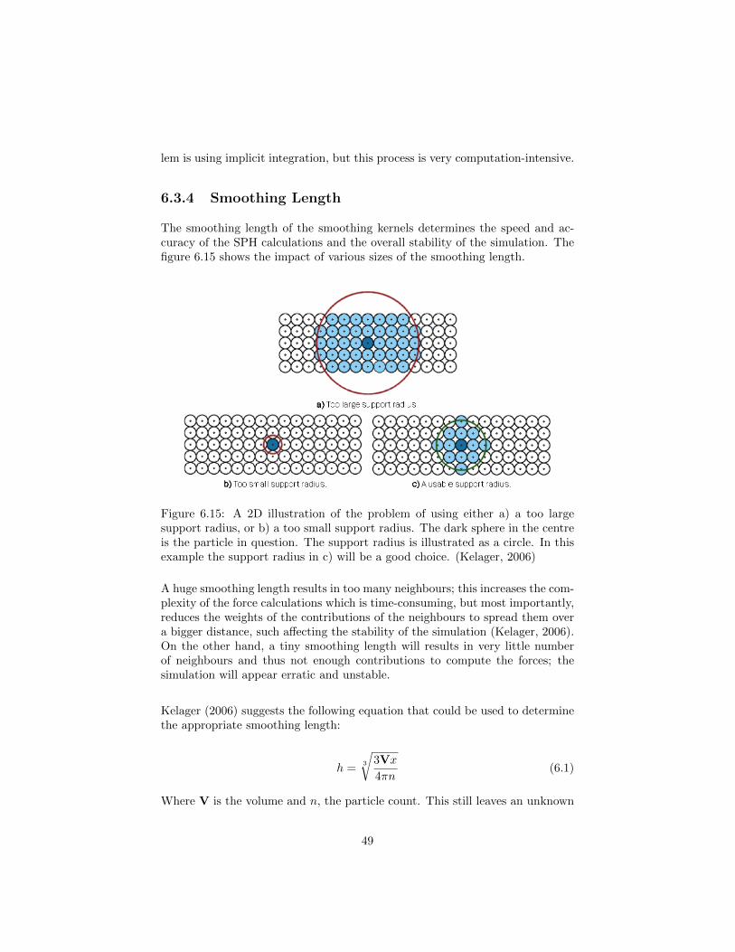
The smoothing length of the smoothing kernels determines the speed and ac-curacy of the SPH calculations and the overall stability of the simulation. Thefigure 6.15 shows the impact of various sizes of the smoothing length.

Figure 6.15: A 2D illustration of the problem of using either a) a too largesupport radius, or b) a too small support radius. The dark sphere in the centreis the particle in question. The support radius is illustrated as a circle. In thisexample the support radius in c) will be a good choice. (Kelager, 2006)

A huge smoothing length results in too many neighbours; this increases the com-plexity of the force calculations which is time-consuming, but most importantly,reduces the weights of the contributions of the neighbours to spread them overa bigger distance, such affecting the stability of the simulation (Kelager, 2006).On the other hand, a tiny smoothing length will results in very little numberof neighbours and thus not enough contributions to compute the forces; thesimulation will appear erratic and unstable.

Kelager (2006) suggests the following equation that could be used to determinethe appropriate smoothing length:

h =3

√3Vx

4πn(6.1)

Where V is the volume and n, the particle count. This still leaves an unknown

49

x which is the number of neighbours desired. The aim would be to keep x smallto reduce the calculation complexity, while still getting a stable simulation.

For the simulations done in this project, the smoothing length has been set as0.3, which is roughly near to the result of the formula, described previously,when x = 10.

6.3.5 Performance And Efficiency

In this section, the performance of the solver was observed over various amountsof particles, in terms of memory and CPU usage. The aim is to get a linearrelationship between these metrics and the particle count, so as to get as closeas possible to a complexity of O(n).

6.3.5.1 First Approach to Neighbour Search optimisation

Among all the tasks that are executed in the simulation loop, the searching ofneighbours for a particle is most complex and resource-intensive. This is due tothe numerous mathematical operations, such as mod and xor, that need to beperformed to hash the positions, iterate over a bounding box to get neighboursand check for duplicates. This routine need to be executed for every single par-ticle in the simulation and at every iteration. The situation is worsened by thefact that the neighbours need to be calculated twice, as demonstrated in section5.1, one for the calculation of the density and the other for the actual forcecalculation. Therefore, the optimisation of the neighbour search would result ina drastic performance gain.

Two methods of querying the neighbours are considered. The first one is toquery the latter on the fly, i.e., get the neighbours at the time they are needed,thus inevitably calculating the neighbours twice. The second method is to getthe neighbours of all the particles and save them to a big neighbour list,prior to all other tasks, then use the neighbours from this big list (which is asimple fetch from a list) for the density calculation and force calculation. Thislatter method, thus, eliminates the need for double calculations and results in aperformance boost. Two simulations are run, one with a particle count of 13566and the other with a particle count of 29667, over 3000 iterations using thesetwo methods alternatively and observing their execution time (figure 6.16).

The graph 6.16 demonstrates the performance boost obtained by using the sec-ond method. While the execution time scales accordingly for the 13566 particlecount over the 3000 iterations, it increases non-linearly as the number of parti-cles is increased, i.e., for the 29667 particle count as from the 2000-mark. This

50

Figure 6.16: Execution time (in minutes) over iterations. OTF13 - on thefly with 13566 particles, OTF29 - on the fly with 29667 particles, BNL13 - bigneighbour list with 13566 particles, and BNL29 - big neighbour list with 29667particles.

is due to the fact that the increased particle count increases the number ofneighbours with which each particle interacts as they come close to each otherand this definitely increases the complexity of the force calculations; however,from gradient of the graph remains constant from the 2000-mark to 3000, thusproving a linear complexity.

On the other hand, the memory usage pattern is the total opposite; the on thefly method uses the least amount of memory as compared to the big neighbourlist method, mostly due to the fact that the latter needs storage to keep theneighbours. Since, the neighbour list per particle is totally dynamic, space can-not be reserved in advance and thus the performance of the data structure usedfor the storage degrades with more iterations and particles. This is illustratedin the graph 6.17.

6.3.5.2 CPU usage optimisation using OpenMP

Although a big performance boost was obtained using the big neighbour listmethod, discussed in the previous chapter, the solver still is not fully optimisedand as such cannot be used for big particle counts. The Lagrangian fluid simu-lation is basically a subset of particle systems, where the use of multiple cores isbecoming very popular to reduce the execution time as the complexity increases.

51

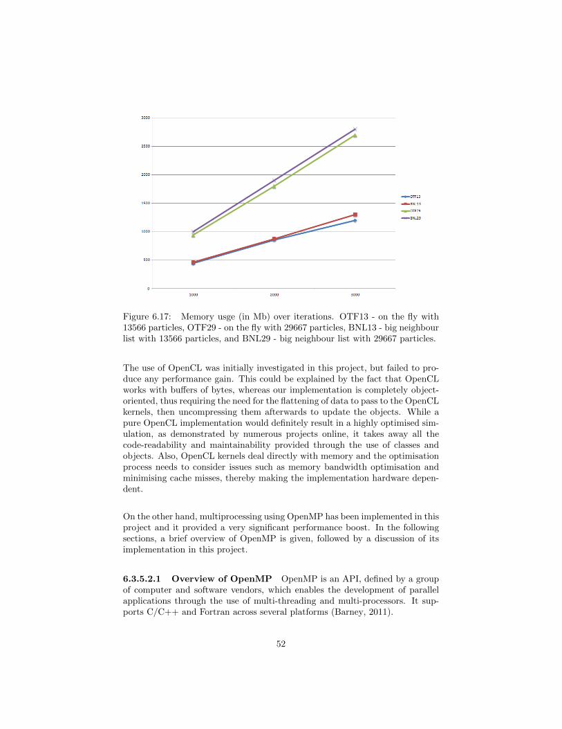
Figure 6.17: Memory usge (in Mb) over iterations. OTF13 - on the fly with13566 particles, OTF29 - on the fly with 29667 particles, BNL13 - big neighbourlist with 13566 particles, and BNL29 - big neighbour list with 29667 particles.

The use of OpenCL was initially investigated in this project, but failed to pro-duce any performance gain. This could be explained by the fact that OpenCLworks with buffers of bytes, whereas our implementation is completely object-oriented, thus requiring the need for the flattening of data to pass to the OpenCLkernels, then uncompressing them afterwards to update the objects. While apure OpenCL implementation would definitely result in a highly optimised sim-ulation, as demonstrated by numerous projects online, it takes away all thecode-readability and maintainability provided through the use of classes andobjects. Also, OpenCL kernels deal directly with memory and the optimisationprocess needs to consider issues such as memory bandwidth optimisation andminimising cache misses, thereby making the implementation hardware depen-dent.

On the other hand, multiprocessing using OpenMP has been implemented in thisproject and it provided a very significant performance boost. In the followingsections, a brief overview of OpenMP is given, followed by a discussion of itsimplementation in this project.

6.3.5.2.1 Overview of OpenMP OpenMP is an API, defined by a groupof computer and software vendors, which enables the development of parallelapplications through the use of multi-threading and multi-processors. It sup-ports C/C++ and Fortran across several platforms (Barney, 2011).

52

OpenMP is based on a shared-memory model (Adve and Gharachorloo, 1996),with multiple threads are created and allocated jobs and shared memory spaceis used to synchronise the result of their execution. As such, it uses the conceptof private and shared memory variables and makes a clear distinction betweenthese two. Care should be taken when using shared memory to prevent raceconditions, with different threads overwriting the shared variable each in theirturn and resulting in an undetermined state for the shared variable.

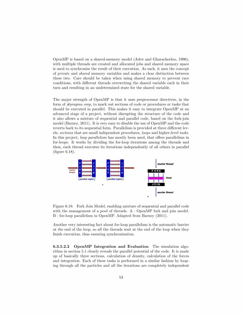
The major strength of OpenMP is that it uses preprocessor directives, in theform of #pragma omp, to mark out sections of code or procedures or tasks thatshould be executed in parallel. This makes it easy to integrate OpenMP at anadvanced stage of a project, without disrupting the structure of the code andit also allows a mixture of sequential and parallel code, based on the fork-joinmodel (Barney, 2011). It is very easy to disable the use of OpenMP and the codereverts back to its sequential form. Parallelism is provided at three different lev-els; sections that are small independent procedures, loops and higher-level tasks.In this project, loop parallelism has mostly been used, that offers parallelism infor-loops. It works by dividing the for-loop iterations among the threads andthen, each thread executes its iterations independently of all others in parallel(figure 6.18).

Figure 6.18: Fork Join Model, enabling mixture of sequential and parallel codewith the management of a pool of threads. A : OpenMP fork and join model.B : for-loop parallelism in OpenMP. Adapted from Barney (2011).

Another very interesting fact about for-loop parallelism is the automatic barrierat the end of the loop, so all the threads wait at the end of the loop when theyfinish execution, thus ensuring synchronisation.

6.3.5.2.2 OpenMP Integration and Evaluation The simulation algo-rithm in section 5.1 clearly reveals the parallel potential of the code. It is madeup of basically three sections, calculation of density, calculation of the forcesand integration. Each of these tasks is performed in a similar fashion by loop-ing through all the particles and all the iterations are completely independent

53

from each other, thus facilitating the use of OpenMP.

Algorithm 7: Modified algorithm to perform simulation of fluid using OpenMPdirectives

while timer ticks doRefresh neighbour search structure

#pragma omp forforeach particle P in particle list do

Calcule the density and pressure of Pend#pragma omp forforeach particle P in particle list do

Calculate net force of PIntegrate acceleration to get velocity v and position xApply collision detection and resolution on P against environmentMove P and render it

end

end

The performance of the OpenMP integration was observed (figure 6.19), onceagain, using the two methods, on the fly and big neighbour list for neighboursearch, discussed earlier in section 6.3.5.1.

The results, from figure 6.19, proved to be totally opposite of what was demon-strated in the previous graphs. Here, the on the fly method proved to be thefastest with performance boost of up to 3 times, while the big neighbour listwas totally inefficient and sometimes even slower. This latter delay can be ex-plained by the fact that the big list becomes a shared object when used withOpenMP; as such, the OpenMP ordered construct must be used to ensure thatit is updated by only one thread at a time and that too in order. All this syn-chronisation among threads impaired their parallel working and slowed downthe execution. As for the former case, the performance gained was because ofthe use of the three other processors (the simulation computer is a quad-coremachine) resulting in a CPU usage of around 325 - 400 % as compared to theinitial 96 - 100 %.

In this project, the on the fly neighbour search method was finally chosenwith OpenMP integration. The graph 6.20 demonstrates the performance gainby using OpenMP.

54

Figure 6.19: Execution time (in minutes) over iterations using OpenMP.OTF13 - on the fly with 13566 particles, OTF29 - on the fly with 29667 particles,BNL13 - big neighbour list with 13566 particles, and BNL29 - big neighbour listwith 29667 particles.

Figure 6.20: Execution time (in minutes) of 13566 particles over 3000 iterationsusing OpenMP and the on the fly method for neighbour search.

55

Chapter 7

Conclusion

In this project, a Lagrangian simulation of liquids has been implemented usingthe SPH method. In this section, an analysis of the success of the projectis made, followed by a discussion of some problems encountered during theimplementation and some improvements and future work.

7.1 Critical Analysis

Overall, this project has been successful as it meets all of the objectives initiallyset in the Design chapter 4.1. Features such as particle injection have broughtin some very interesting results as shown in section 6.2.6. The interaction be-tween the fluids and the rigid bodies has been another very successful objectiveachieved in this project and some very interesting scenarios are demonstratedwith great success in section 6.2.3. The interaction between multiple fluids isinherent in Lagrangian particle-based methods and has proved to work reallywell in this project as demonstrated in section 6.2.2. The functionality of ex-porting the simulation data to Houdini has also been implemented and beingable to manipulate it in Houdini gives much freedom for advanced enhancementand rendering. The use of multiprocessing and OpenMP has also been success-fully used in this project to give a significant performance boost. Efficient useof memory and coding practices have been adopted, such as the use of passingvalues by reference to prevent the creation of object copies while easily passaddresses around and fast memory access achieved through contiguous memoryallocation on the stack instead of resorting to pointers on the heap.

On the other hand, the simulation of the flow of various liquids present somechallenges since the parameters cannot be tweaked over a wide range of values.While the basic liquid has been successfully simulated and used for most of thesimulations presented in this paper, tweaking the parameters such as viscositydoes not always guarantee a stable simulation, as discussed in section 6.3; aslong as the timestep is kept really small, the simulation is assumed to be stable.

7.2 Problems Encountered

The density calculation of the particles is quite problematic because it dependshighly on the accuracy on the neighbour search spatial algorithm and any fluc-

56

tuation in the latter impacts the density value, the resulting pressure and thewhole of the SPH force calculations. At several instances, the simulation wouldexplode without any apparent reason; the cause was eventually traced back toan abnormality in the neighbour search procedure and this debugging processwas quite painful. Another issue with SPH density calculation is that surfaceparticles have less neighbours than those in the middle of the fluid; thus theirdensities are wrongly calculated, resulting in visual artifacts at the surface ofthe fluid, such as a massive concentration of particles stuck together at the edgeof the boundary. Lerer, among many others, proposes solutions to solve thisproblem.Another significant problem, that has been encountered, is with the neighboursearch algorithm. Spatial hashing uses a smoothing length and thus divides thespace in small cells; this, however, is rendered totally useless as the number ofparticles increases. In the latter case, the cell size remains constant and thus thenumber of neighbours per cell returned is massive and increases the complex-ity of the force calculations. At one point during the testing phase, a massiveneighbour count of nearly 900 was returned and this resulted in a definite halt inthe simulation, as the forces were calculated over 900 particles. To resolve thisissue, the boundary dimension was increased so that the fluid particles do notcome too close to each other. However, many papers have studied this problemand the most popular solution is to use adaptive smoothing length, whereby thesmoothing length and thus the cell size is adjusted accordingly to the simulationspace.

7.3 Improvements and Future work

While SPH is an easy method to understand and implement, it poses a lot ofchallenges that must be addressed to ensure that good simulations are obtained,as discussed in section 6.3. Improvements could be made to address a numberof these issues. Alternate formulas, such as the Tait’s equation (Monaghan,1994), could be used to calculate the density and pressure with better accuracy.The high compressibility issues could be resolved with the use of the conjugategradient method (Becker and Teschner, 2007). Furthermore, the timestep limitcould be resolved by using implicit integration methods as discussed by Stam(1999). SPH provides a lot of room for improvement so that much more stablesimulation can be achieved. Once the latter is achieved, various types of liquidcan then be easily simulated such as honey and ink.The nature of this project has a big scope for future work. Some of theseare discussed briefly in this paragraph. Future work could be done on theuser interface to allow easy tweaking of the simulation fluids. Concerning therepresentation of rigid bodies, the use of polygon meshes would be considered inthe future because they provide much more complex shapes as compared to thecurrently being used implicit functions. This would enable much more complexand interesting scenarios such as the flow of fluid in blood vessels and etc. The

57

performance of the simulation algorithm would be another concern for futurework. Improvement, in terms of frame-rate-per-second, would be consideredusing other alternative technologies such as MPI to add in much more processingpower or even OpenCL. Since the weakness of the spatial hashing with massiveparticle count has been discussed in the previous paragraph, some future workwould definitely involve the use of a more efficient neighbour search algorithmdesigned to handle a much larger particle count, however close they get to eachother, or even improve the existing spatial hashing algorithm to tackle thisspecific problem. The implementation of the reaction of fluid particle forces onthe rigid bodies would also be a good consideration as a future work, so thatNewton’s third law of motion, action and reaction, is respected and thus a morestable simulation could be expected. This could also be then used to implementfloating bodies on the surface of the fluid or enable more complex scenarios suchas the opening of a valve by the pressure exerted by the simulated fluid.

58

References

Adve, S. V. and Gharachorloo, K. (1996). Shared memory consistency models:A tutorial. Computer, 29:66–76. Available from: http://www.hpl.hp.com/

techreports/Compaq-DEC/WRL-95-7.pdf [Accessed 19 Aug 2011].

Angst, R. (2007). Fluid effects in cutting simulations. Semester thesis, SwissFederal Institute Of Technology, Zurich. Available from: http://www.

inf.ethz.ch/personal/rangst/publications/ST07.pdf [Accessed 19 Aug2011].

Auer, S. (2008). Realtime particle-based fluid simulation. Mas-ter’s thesis, Technical University Munich. Available from: http:

//www.google.co.uk/url?sa=t&source=web&cd=2&ved=0CCIQFjAB&url=

http%3A%2F%2Ffluid-particles.googlecode.com%2Ffiles%

2Frealtime%2520particle%2520based%2520fluid%2520simulation%

2520-%2520thesis.pdf&rct=j&q=Realtime%20particle-based%

20fluid%20simulation%20auer&ei=3AxOTqiLFIeHhQf7qMDeBg&usg=

AFQjCNH6qXUW7Pi-jNjsuOAOo3h0LrQYgA&sig2=cZm71gZz7Q0pTAmq-9WD-A

[Accessed 19 Aug 2011].

Barney, B. (2011). Openmp. Technical report, Lawrence Livermore NationalLaboratory. Available from: https://computing.llnl.gov/tutorials/

openMP/ [Accessed 19 Aug 2011].

Becker, M. and Teschner, M. (2007). Weakly compressible sph for free surfaceflows. In Proceedings of the 2007 ACM SIGGRAPH/Eurographics symposiumon Computer animation, SCA ’07, pages 209–217, Aire-la-Ville, Switzerland,Switzerland. Eurographics Association.

Bell, N., Yu, Y., and Mucha, P. J. (2005). Particle-based simulation of granularmaterials. In Proceedings of the 2005 ACM SIGGRAPH/Eurographics sym-posium on Computer animation, SCA ’05, pages 77–86, New York, NY, USA.ACM.

Bridson, R. and Muller-Fischer, M. (2007). Fluid simulation: Siggraph 2007course notes. In ACM SIGGRAPH 2007 courses, SIGGRAPH ’07, pages1–81, New York, NY, USA. ACM.

Carlson, M., Mucha, P. J., Van Horn, III, R. B., and Turk, G. (2002). Melt-ing and flowing. In Proceedings of the 2002 ACM SIGGRAPH/Eurographicssymposium on Computer animation, SCA ’02, pages 167–174, New York, NY,USA. ACM.

Clavet, S., Beaudoin, P., and Poulin, P. (2005). Particle-based viscoelasticfluid simulation. In Proceedings of the 2005 ACM SIGGRAPH/Eurographicssymposium on Computer animation, SCA ’05, pages 219–228, New York, NY,USA. ACM.

59

Desbrun, M. and Cani, M.-P. (1996). Smoothed Particles: A new paradigm foranimating highly deformable bodies. In Boulic, R. and Hegron, G., editors,Eurographics Workshop on Computer Animation and Simulation (EGCAS),pages 61–76, Poitiers, France. Springer-Verlag. Published under the nameMarie-Paule Gascuel.

Fan, Z., Qiu, F., Kaufman, A., and Yoakum-Stover, S. (2004). Gpu clus-ter for high performance computing. SC Conference, 0:47. Availablefrom: http://www.cs.sunysb.edu/~vislab/papers/GPUcluster_SC2004.

pdf [Accessed 19 Aug 2011].

Gingold, R. and Monaghan, J. (1982). Kernel estimates as a basis for gen-eral particle methods in hydrodynamics. Journal of Computational Physics,46(3):429 – 453.

Harada, T., Koshizuka, S., and Kawaguchi, Y. (2007). Smoothed particle hy-drodynamics on gpus. In Proc. of Computer Graphics International, pages63–70.

Harris, M. J. (2003). Real-time cloud simulation and rendering. PhD thesis.Available from: http://citeseerx.ist.psu.edu/viewdoc/download?doi=

10.1.1.5.7402&rep=rep1&type=pdf [Accessed 19 Aug 2011].

Hoetzlein, R. and Hollerer, T. (2009). Interactive water streams with spherescan conversion. In Proceedings of the 2009 symposium on Interactive 3Dgraphics and games, I3D ’09, pages 107–114, New York, NY, USA. ACM.

Horvath, P. and Illes, D. (2007). Sph-based fluid simulation for special effects.In The 11th Central European Seminar on Computer Graphics. Avail-able from: http://www.cg.tuwien.ac.at/hostings/cescg/CESCG-2007/

papers/TUBudapest-Horvath-Peter/TUBudapest-Horvath-Peter.pdf

[Accessed 19 Aug 2011].

Hut, P. and Makino, J. (2004). The art of computational science. Avail-able from: http://www.artcompsci.org/kali/vol/two_body_problem_2/

ch02.html#rdocsect8 [Accessed 19 Aug 2011].

Kelager, M. (2006). Lagrangian fluid dynamics using smoothed particle hy-drodynamics. Available from: http://image.diku.dk/projects/media/

kelager.06.pdf [Accessed 19 Aug 2011].

Kolb, A. and Cuntz, N. (2005). Dynamic particle coupling for gpu-based fluidsimulation. In In Proc. of the 18th Symposium on Simulation Technique,pages 722–727.

Lerer, A. 3-dimensional fluid simulation with smoothed particle hydrodynam-ics. Available from: http://web.mit.edu/alerer/www/sph.pdf [Accessed19 Aug 2011].

Lucy, L. (1977). A numerical approach to the testing of the fission hypothesis.Astronomical Journal, 82:1013–1024.

60

Macey, J. (2010). Ngl graphics library. Available from: http://nccastaff.

bournemouth.ac.uk/jmacey/GraphicsLib/ [Accessed 19 Aug 2011].

Miller, G. and Pearce, A. (1989). Globular dynamics: A connected particlesystem for animating viscous fluids. Computers & Graphics, 13(3):305 – 309.

Monaghan, J. J. (1994). Simulating free surface flows with sph. Journal ofComputational Physics, 110(2):399 – 406.

Monaghan, J. J. (2005). Smoothed particle hydrodynamics. Reports on Progressin Physics, 68(8):1703–1759.

Muller, M., Charypar, D., and Gross, M. (2003). Particle-based fluid simu-lation for interactive applications. In Proceedings of the 2003 ACM SIG-GRAPH/Eurographics symposium on Computer animation, pages 154–159.Eurographics Association.

Muller, M., Solenthaler, B., Keiser, R., and Gross, M. (2005). Particle-based fluid-fluid interaction. In Proceedings of the 2005 ACM SIG-GRAPH/Eurographics symposium on Computer animation, pages 237–244.ACM.

Paiva, A., Petronetto, F., Lewiner, T., and Tavares, G. (2009). Particle-basedviscoplastic fluid/solid simulation. Computer-Aided Design, 41(4):306–314.

Pelfrey, B. (2010). An informal tutorial on smoothed particle hydrodynamicsfor interactive simulation. Available from: http://www.cs.clemson.edu/

~bpelfre/sph_tutorial.pdf [Accessed 19 Aug 2011].

Premoze, S., Tasdizen, T., Bigler, J., Lefohn, A., and Whitaker, R. T.(2003). Particle-based simulation of fluids. Computer Graphics Forum,22(3):401–410. Available from: http://www.sci.utah.edu/~tolga/pubs/

ParticleFluidsHiRes.pdf [Accessed 19 Aug 2011].

Priscott, C. (2010). 3d langrangian fluid solver using sph approxima-tions. Master’s thesis, Bournemouth University, NCCA. Availablefrom: http://nccastaff.bournemouth.ac.uk/jmacey/MastersProjects/

MSc2010/08ChrisPriscott/ChrisPriscott_THESIS.pdf [Accessed 19 Aug2011].

Reeves, W. T. (1983). Particle systems : a technique for modeling a class offuzzy objects. ACM Trans. Graph., 2:91–108.

Stam, J. (1999). Stable fluids. In Proceedings of the 26th annual con-ference on Computer graphics and interactive techniques, pages 121–128.ACM Press/Addison-Wesley Publishing Co. Available from: http://www.

dgp.toronto.edu/people/stam/reality/Research/pdf/ns.pdf [Accessed19 Aug 2011].

Stam, J. and Fiume, E. (1995). Depicting fire and other gaseous phenomenausing diffusion processes. In Proceedings of the 22nd annual conference on

61

Computer graphics and interactive techniques, SIGGRAPH ’95, pages 129–136, New York, NY, USA. ACM.

Steele, K., Cline, D., Egbert, P. K., and Dinerstein, J. (2004). Modeling andrendering viscous liquids: Research articles. Comput. Animat. Virtual Worlds,15:183–192.

Succi, S., Benzi, R., and Higuera, F. (1991). The lattice boltzmann equation: Anew tool for computational fluid-dynamics. Physica D: Nonlinear Phenomena,47(1-2):219 – 230.

Takeshita, D., Ota, S., Tamura, M., Fujimoto, T., Muraoka, K., and Chiba,N. (2003). Particle-based visual simulation of explosive flames. ComputerGraphics and Applications, Pacific Conference on, 0:482.

Teschner, M., Heidelberger, B., Muller, M., Pomeranets, D., and Gross,M. (2003). Optimized spatial hashing for collision detection of de-formable objects. In Proceedings of Vision, Modeling, VisualizationVMV03, pages 47–54. Available from: http://www.beosil.com/download/

CollisionDetectionHashing_VMV03.pdf [Accessed 19 Aug 2011].

Umenhoffer, T. and Szirmay-Kalos, L. (2008). Interactive distributed fluid sim-ulation on the gpu. Technical report, Budapest University of Technology andEconomics. Available from: http://sirkan.iit.bme.hu/~szirmay/fluid.pdf [Accessed 19 Aug 2011].

WikimediaCommons (2011). Sine(sin)-function. Available from: http://

commons.wikimedia.org/wiki/Image:Sine.svg [Accessed 19 Aug 2011].

62