44
1 ENSIM 3A L’intensité de structure Jean-Claude Pascal LAUM, ENSIM

1
ENSIM 3A
L’intensité de structure
Jean-Claude Pascal
LAUM, ENSIM

2
ENSIM 3A
Plan
� Expression de l’intensité dans les poutres
� Formulation approchée
� La mesure

3
ENSIM 3A
Expression de l’intensité de structure
Expression de l’intensité de structure
L’intensité structurale ou vibratoire correspond à la densité de flux de
puissance [en W/m2] transporté par les ondes vibratoires
densité de force (tenseur des contraintes) x vecteur vitesse
L’intensité moyenne dans le temps
avec les grandeurs complexes et
( ) ( ) ( ) 3,2,1, =−= ∑ jitwttij
jiji&σ
( ) { }∑ ∗−==
j
jijii wtiI &σRe2
1
( ) { }tj
ijij etωσσ Re= ( ) { }
jj wtw &Re=

4
ENSIM 3A
L’intensité structurale des ondes de flexion dans une poutre se réduit à
[W]
Définition de l’intensité des ondes de flexion
Expression de l’intensité des ondes de flexion
( ) ( ) ( ) ( ) ( ){ }xxMxwxQxI∗∗ +−= θ&&Re
2
1
La théorie d’Euler–Bernouilli permet d’exprimer toutes les quantités à
partir du déplacement
� déplacement angulaire
� moment de flexion
� effort tranchant
avec
( ) ( )
( ) ( )
( ) ( )3
3
2
2
x
xwEIxQ
x
xwEIxM
x
xwx
∂
∂−=
∂
∂=
∂
∂=θ
( ) ( ) ( ) ( ) ( )
∂
∂
∂
∂−
∂
∂=
∗∗
x
xw
x
xwxw
x
xwEIxI
&&&
&
2
2
3
3
Im2ω
ωjww &=

5
ENSIM 3A
Utilisation des différences finies pour exprimer les dérivées spatiales
Intensité approchée par différence finie
( ) ( )3
1234
3
3
2
1234
2
2
2312
33
2
2
x
wwww
x
w
x
wwww
x
wx
ww
x
wwww
∆
−+−≈
∂
∂
∆
+−−≈
∂
∂∆
−≈
∂
∂+≈
&&&&&&&&&&
&&&&&&
x
x∆
1 2 3 4
( ){ }∗∗∗ −−
∆≈ 4231323
4Im4
wwwwwwx
EII &&&&&&
ω
ωjww &&& =( )
{ }∗∗∗ −−∆
≈⇒ 423132334Im
4wwwwww
x
EII &&&&&&&&&&&&
ω
Expression de l’intensité des ondes de flexion

6
ENSIM 3A
Expression générale du déplacement
avec le nombre d’onde de flexion
En champ lointain quand il n’y a pas d’ondes évanescentes
Approximation de champ lointain
⇒= ωjww &&&
Expression de l’intensité des ondes de flexion
( ) kxjkxkxjkxeAeAeAeAxw 4321 +++= −−
4
EI
Ak
ρω=
x
wk
x
wwk
x
w
∂
∂−≈
∂
∂−≈
∂
∂ &&&
& 2
3
32
2
2
{ }∗∗
∆≈→
∂
∂≈ 21ImIm2 ww
x
AEII
x
wwAEII &&
&&
ρρ
{ }∗
∆≈ 212
Im wwx
AEII &&&&
ω
ρx∆
1 2
7
ENSIM 3A
CHARACTERISATION OF A DISSIPATIVE ASSEMBLY
BY STRUCTURAL INTENSITY
A. How to calculate energetic quantities from laser
vibrometer measurements
B. Analysis of assembly plate using energetic
quantities
C. Transformation of 2D model to 1D junction model
D. Use energy conservation low to compute joint
dissipation

8
ENSIM 3A
MEASURED ENERGETIC QUANTITIES
Force distribution
Divergence of the
structural intensity
Potential energy
density
Kinetic energy
density
Structural intensity
{ }∗∇=⋅∇ vvB 4Im
2ωI
( ) ( ) ( )( )yxvkyxvj
ByxF B ,,, 44 −∇
=
ω
4
2v
hT ρ=
( )
∂∂
∂−
∂
∂
∂
∂−−∇=
∗ 22
2
2
2
222
2Re12
4 yx
v
y
v
x
vv
BV ν
ω
( ) ( )
∇×∇×∇−
−∇∇−∇∇= ∗∗∗vvvvvv
B
2
1Im
2
22 υ
ωI

9
ENSIM 3A
MEASURED ENERGETIC QUANTITIES :
ADVANCED METHODS OF WAVENUMBER PROCESSING
Use of SFT for calculation of spatial derivatives
( )),()()(
,yx
ny
mx
TF
nm
nm
kkVjkjkyx
yxv−−
∂∂
∂ +
a
is the Spatial Fourier Transform of ),( yx kkV ( )yxv ,
y
x
SFT
xkyk
( )yxv , ),( yx kkV
SFT on truncated signals amplifies the components of high wavenumbers, bringing large contributions of the high wavenumber components to the results, especially in the case of the high-order derivatives of the velocity.
The derivatives of vibrating velocity are easily calculated by

10
ENSIM 3A
Mirror methods used to reduce errors caused by operation of SFT
The idea of the mirror method is to build a continuous and
periodic signal (the resulting signal) from the signal to be
processed by SFT (the original signal).
-0.2 -0.1 0 0.1 0.2 0.3 0.4 0.5 0.60
0.5
1
1.5
2
2.5
3
3.5
4
4.5
5x 10
-5
Amplitude
Signa l
dis ta nce (m)
Mirror s ignal + Origina l s ignalOrigina l s ignal
MEASURED ENERGETIC QUANTITIES :
ADVANCED METHODS OF WAVENUMBER PROCESSING

11
ENSIM 3A
EXPERIMENTAL CONFIGURATION
93
0
mm
850 mm
20 m
m
clampededge
free edge
x
y
� A scanning vibrometer use a OFV
300 optical head
� Two galvo-driven mirrors direct the
laser beam horizontally and vertically
� 32x32 measurement points
� Test assembly consists of two steel
plates of thickness 1 mm
� The two opposite edges are clamped.
The two other edges are free
� A normal point force is acting on the plate

12
ENSIM 3A
ASSEMBLY PLATE ANALYSIS :
STRUCTURAL INTENSITY
� Wavenumber processing was used
� Data integrated over a frequency band of 525 to 1000 Hz
AIII A ×∇+∇−=+= φφ
Standard structural
intensity
Irrotational structural
intensity

13
ENSIM 3A
Force s F=668 HzDivergence of the structural intensity Force distribution
At frequency 668 Hz. these two quantities show that the dissipation produced by the joint is maximum at the positions where the joint is constrained by the tightening of the bolts
ASSEMBLY PLATE ANALYSIS :
INJECTED OR DISSIPATED POWER AND FORCE DISTRIBUTION

14
ENSIM 3A
ASSEMBLY PLATE ANALYSIS :
FORCE DISTRIBUTIONS AVERAGED IN FREQUENCY BAND
[549,600] Hz [601,649] Hz [650,699] Hz [700,750] Hz
[751,800] Hz [801,850] Hz [851,900] Hz [901,950] Hz
The dominating zones of dissipation correspond to the points of maximum constraints introduced by the bolts ensuring the contact of the two parts of the plate on the joint. However this behaviour of the
joint will depend largely on the frequency

15
ENSIM 3A
EQUIVALENT 1D MODEL :
AVERAGED POWER FLOW ON PLATE
x
y0
forc
e
Plate
1
Plate 2join
t( ) ( )∫=Ly
xx dyyxIx
0
,φ( ) ( )∫=
Lx
yy dxyxIy0
,φ
Total power flow in x-
direction Total power flow in y-direction

16
ENSIM 3A
The evolution of the
averaging power flow over
one direction of a plate
reveals the similar
behaviour to that of a one-
dimensional system like a
beam in the other direction
of the plate
F
Beam
EQUIVALENT 1D MODEL :
ONE-DIMENTIONAL BEAM-LIKE MODEL

17
ENSIM 3A
� The basic idea is thus to represent the joint like a node of
junction of one-dimensional elements
� The third branch comprising only an outgoing wave is used to
express the power dissipated by the joint. Thus the power of each
branch entering in the junction element can respectively be
written by
EQUIVALENT 1D MODEL :
ONE-DIMENTIONAL BEAM-LIKE MODEL
+2a
+1a
plate 1 junction plate 2
−2a
−3a
−1a
−= −+ 2
1
2
121
1 aaP
2
321
3−−= aP
−= −+ 2
2
2
221
2 aaP

18
ENSIM 3A
plate 1 junction
plate 2
2P
3P
1P
Expression of the
conservation of flow
“entering” in the junction
0321 =++ PPP
2
2123
eetcP dg
+−≈
An approximation of the dissipated
power
=
+
+
−
−
−
2
1
3
2
1
a
a
t
r
t
t
t
r
a
a
a
dd
Far-field scattering matrix
gc the group velocity for the flexural waves
dt the dissipation coefficient
21, ee the densities of total energy on both sides of the junction
the reflection and transmission coefficientstr,
EQUIVALENT 1D MODEL :
ONE-DIMENTIONAL BEAM-LIKE MODEL
19
ENSIM 3A
USE ENERGY CONSERVATION LAW
TO COMPUTE JOINT DISSIPATION
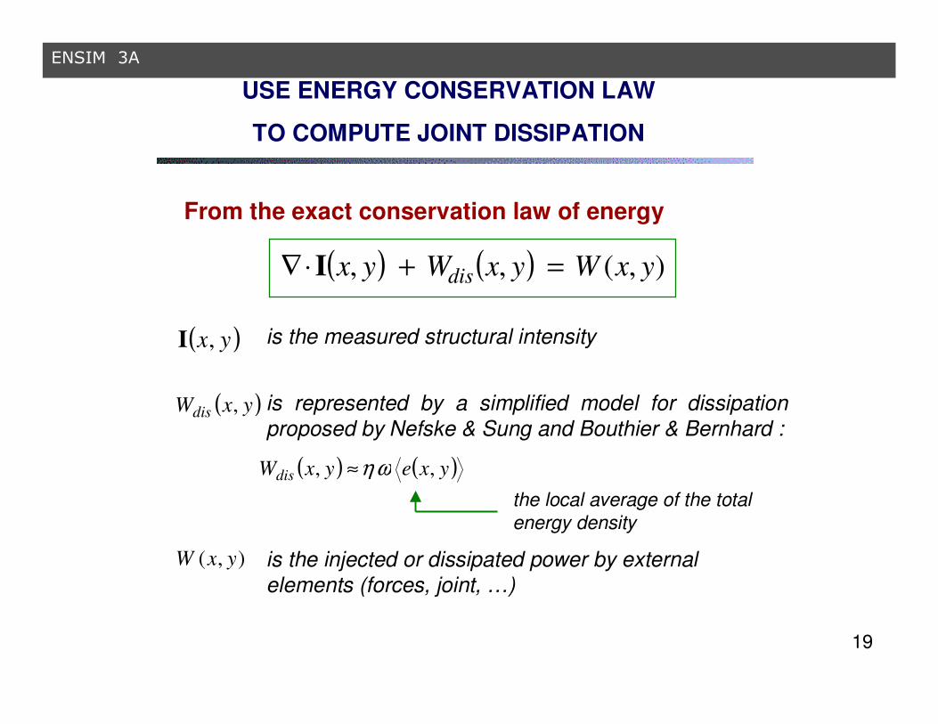
From the exact conservation law of energy
( ) ( ) ),(,, yxWyxWyx dis =+⋅∇ I
( )yx,I
( )yxWdis ,
),( yxW
is the measured structural intensity
is represented by a simplified model for dissipation
proposed by Nefske & Sung and Bouthier & Bernhard :
( ) ( )yxeyxWdis ,, ωη≈
the local average of the total
energy density
is the injected or dissipated power by external
elements (forces, joint, …)
20
ENSIM 3A
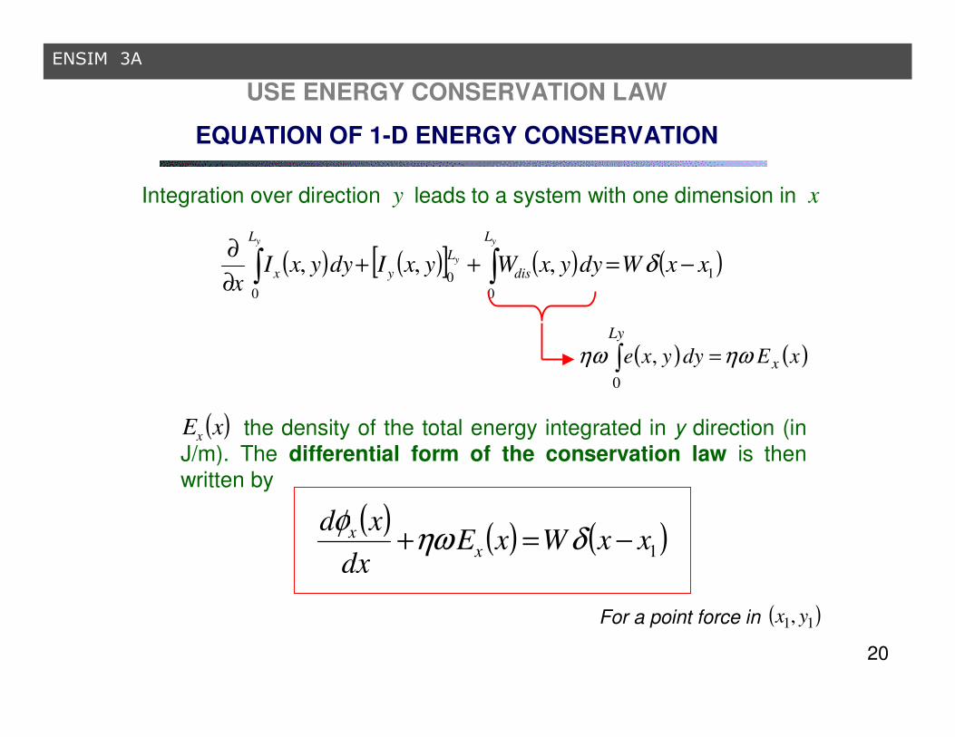
Integration over direction y leads to a system with one dimension in x
( ) ( ) ( )1xxWxEdx
xdx
x −=+ δωηφ
the density of the total energy integrated in y direction (in
J/m). The differential form of the conservation law is then
written by
( )xEx
( ) ( )[ ] ( ) ( )1
0
0
0
,,, xxWdyyxWyxIdyyxIx
y
y
y L
dis
L
y
L
x −=++∂
∂∫∫ δ
( ) ( )xEdyyxe x
Ly
ωηωη =∫0
,
USE ENERGY CONSERVATION LAW
EQUATION OF 1-D ENERGY CONSERVATION
For a point force in ( )11, yx

21
ENSIM 3A
( ) ( ) xEdxxxWx x
x
x ηωδφ −−= ∫0
1
( ) ( ) ( )1xxWxE
dx
xdx
x −=+ δωηφ
x x
( )1xxW −δ
W 0
1xxL
( )xxφ
0 1x xL
Injected power in the plate The evolution of the averaged power
flow along the x dimension
� For an isolated plate system, the boundary conditions
are ( ) ,00 =xφ ( ) 0=−= xxxx LEWL ωηφ
� The loss factor can be estimated
by: ( )∫∫
−==
xx LL
xx
xxdxdyyxe
LE
W
00
minmax
,ω
φφ
ωη
USE ENERGY CONSERVATION LAW
EXEMPLE WITH ONE FORCE

22
ENSIM 3A
0
x
x
0
plate 2plate 1
( ) ( )0xxxEL xy −− δωξ
( )0xEL xyωξ
( )1xxW −δ
W1x
0x xL
xL
USE ENERGY CONSERVATION LAW
ONE FORCE AND JOINT
x
y0
forcePlate 1
Plate 2joint
( )( ) ( ) ( ) ( )01 xxxELxxWxE
dx
xdxyx
x −−−=+ δωξδωηφ
( ) ( ) ( )00201
joint2
xELxExE
LW xyxx
y ωξξω −=+
−=+−
ydg Ltc ωξ 2≡
Use the following differential equation
Dissipated power by joint

23
ENSIM 3A
uppe r part
lowe r part
x01
x02
joint
Position of the joint identified
by the measured forces
( )
( )( ) dydxyxe
LxLe
dydxyxeLx
e
xy
x
L
x
L
yx
L x
y
∫∫
∫ ∫
+
−
−>=<
>=<
ε
ε
0
0
,1
,1
002
0 001
The average density of energy in each of the two
plates:
The loss factor
xx
xx
LEω
φφη minmax
−=
The linear loss factor of density of dissipation
( ) ( )[ ]( ) 2/21
0201minmax
xxy
xxxxx
EEL
xLExE
+
−+−−=
ηωφφξ
At 668 Hz for the plate loss factor and for the linear loss factor of the joint are respectively 0.03 % and 5%
USE ENERGY CONSERVATION LAW
CHARACTERIZATION OF JOINT
24
ENSIM 3A
EFFECTIVE PARAMETER IDENTICAFATION OF 2D
STRUCTURES FROM MEASUREMENTS USING A
SCANNING LASER VIBROMETER
� Introduction
� Methods for evaluating parameters of structures
� Energy methods by using measuring data by a Scanning
Laser Vibrometer
� Estimation of flexural wavebumbers and loss
factor in 2-D structures
� Energy methods to obtain dispersion curve
� General techniques for computation
� Results of measurements from the Scanning Laser Vibrometer

25
ENSIM 3A
Introduction (Introduction (con’tcon’t))
The finite-difference-approximation method
� Use three accelerometers to estimate the flexural
wavenumbers in one-dimensional structures such as
beams
� It is directly based on the wave equation associated
with the far-field approximation
Disadvantage
� Too high sensitivity to phase differences between
sensors due to the use of the finite difference technique
Methods to compute wavenumbers

26
ENSIM 3A
Introduction (Introduction (con’tcon’t))
Methods to compute wavenumbers
Use of Fourier Transform (SFT)
� Determine the maximum of wavenumber spectrum in beams, which
was then used to identify the value of natural flexural wavenumber
� To reduce the distortions brought by Spatial Fourier Transform
(SFT) a regressive method was proposed
Disadvantage
� The use of the direct Fourier Transform results significant errors in
the computations because of truncated signals.

27
ENSIM 3A
Introduction (Introduction (con’tcon’t))
Methods to compute wavenumbers
Spatial correlation approach
� Correlation of the measurements with the wavefield
� The choice of that maximises the correlation gives the
best estimate of the flexural wavenumbers
� It is used for estimation of wavenumbers in 2D structures
Spatial correlation approach
� Correlation of the measurements with the wavefield
� The choice of that maximises the correlation gives the
best estimate of the flexural wavenumbers
� It is used for estimation of wavenumbers in 2D structures
yjkxjk tytx ee−−
tytx kk ,

28
ENSIM 3A
EESTIMATION OF FLEXURAL WAVENUMBER IN STIMATION OF FLEXURAL WAVENUMBER IN
TWOTWO--DIMENSIONAL STRUCTURESDIMENSIONAL STRUCTURES
First step
Use non dissipative energy equation of plate to derive the
effective flexural wavenumbers
29
ENSIM 3A
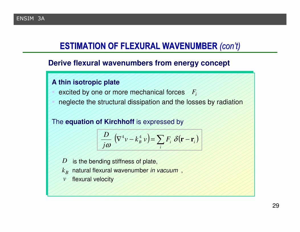
EESTIMATION OF FLEXURAL WAVENUMBER STIMATION OF FLEXURAL WAVENUMBER ((concon’’tt))
A thin isotropic plate
� excited by one or more mechanical forces
� neglecte the structural dissipation and the losses by radiation
The equation of Kirchhoff is expressed by
is the bending stiffness of plate,
natural flexural wavenumber in vacuum ,
flexural velocity
A thin isotropic plate
� excited by one or more mechanical forces
� neglecte the structural dissipation and the losses by radiation
The equation of Kirchhoff is expressed by
is the bending stiffness of plate,
natural flexural wavenumber in vacuum ,
flexural velocity
Derive flexural wavenumbers from energy concept
( ) ( )∑ −=−∇i
iiB Fvkvj
Drrδ
ω44
iF
D
Bk
v

30
ENSIM 3A
EESTIMATION OF FLEXURAL WAVENUMBER STIMATION OF FLEXURAL WAVENUMBER ((concon’’tt))
Derive flexural wavenumbers from energy concept
Multiplying the above equation by the complex conjugate of the velocity yields
{ } 0Im2
4 =∇ ∗vv
D
ω
( ) ( ) ( )
( ) ( )∑
∑
−+=
−=−∇ ∗∗
i
iii
i
iiiB
jQW
vFvkvvj
D
rr
rrr
δ
δω 2
1244
2
Consider a non-dossipation plate. In the zone where there are non-
excitation forces, no damping, no absorptions, we can obtain
two equations:
Leading the divergence of the structural intensity to be zero.
0=⋅∇ sI
31
ENSIM 3A
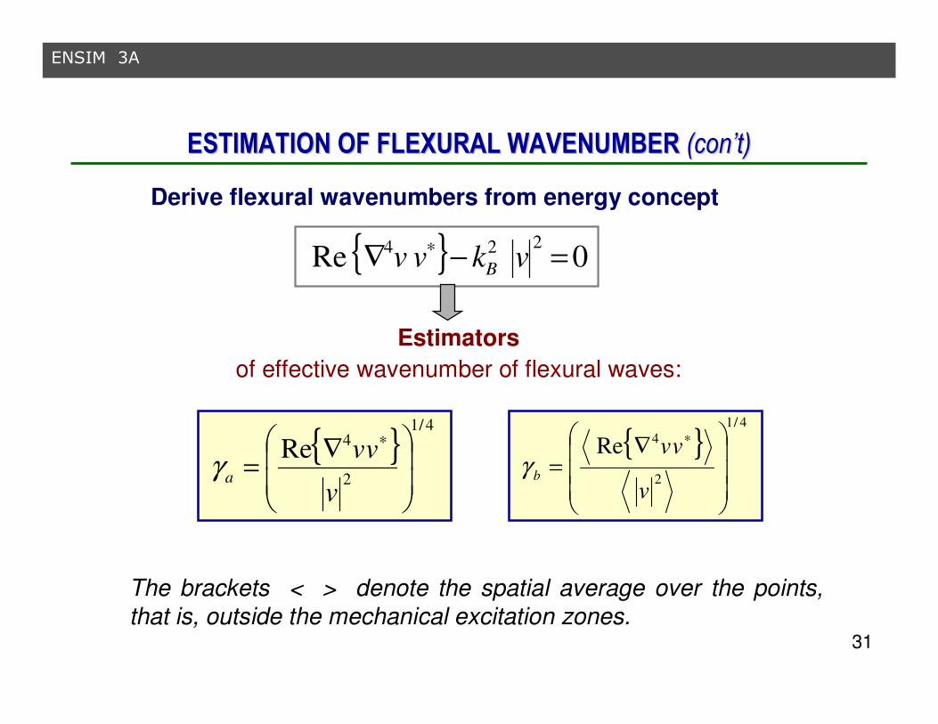
EESTIMATION OF FLEXURAL WAVENUMBER STIMATION OF FLEXURAL WAVENUMBER ((concon’’tt))
Derive flexural wavenumbers from energy concept
{ } 0Re224 =−∇ ∗ vkvv B
Estimators
of effective wavenumber of flexural waves:
{ }4/1
2
4Re
∇=
∗
v
vvaγ
{ }4/1
2
4Re
∇=
∗
v
vvbγ
The brackets < > denote the spatial average over the points,
that is, outside the mechanical excitation zones.

32
ENSIM 3A
CONSIDERATION OF DISSIPATIVE TERMSCONSIDERATION OF DISSIPATIVE TERMS
EFFECTIVE LOSS FACTOREFFECTIVE LOSS FACTOR
Second step
Introduice dissipative terms in plate equation to obtain an estimator of loss factor

33
ENSIM 3A
CONSIDERATION OF DISSIPATIVE TERMSCONSIDERATION OF DISSIPATIVE TERMS
EFFECTIVE LOSS FACTOREFFECTIVE LOSS FACTOR
If the dissipations, losses due to structural dissipation and
losses by radiations, are taken into consideration, equation
of Kirchhoff are expressed by
� is the complex bending stiffness
� the structural loss factor
� is the acoustic radiation pressure on the two sides of the plate
( ) ( )∑ −+−=−∇i
iia FpvhvDj
rrδρωω
241
( )ηjDD += 1
η
ap

34
ENSIM 3A
CONSIDERATION OF DISSIPATIVE TERMSCONSIDERATION OF DISSIPATIVE TERMS
EFFECTIVE LOSS FACTOREFFECTIVE LOSS FACTOR
Assumptions
� non external mechanical forces
� no local damping or absorptions
{ }{ } aT
vv
vvηηη +=
∇
∇−=
*4
*4
Re
Im
Estimator of the total loss factor
• the structural loss factor
• the loss factor due to acoustic
radiations
is radiation efficiency coefficient
η
aη
h
c
vh
Ina ρω
σρ
ωρη 0
22
2==
σ
Maximum Magnitude order
at critical frequency
for brass plate
•
•
4104.9
−×<aη
34105107
−− ×<<× Tη

35
ENSIM 3A
THREE EFFECTIVE ESTIMATORS FOR 2D STRUCTURESTHREE EFFECTIVE ESTIMATORS FOR 2D STRUCTURES
{ }4/1
2
4Re
∇=
∗
v
vvaγ
{ }4/1
2
4Re
∇=
∗
v
vvbγ
{ }{ }*4
*4
Re
Im
vv
vvT
∇
∇−=η
Local WLocal Wavenumberavenumber EstimatorEstimator
AverageAveragedd WWavenumberavenumber EstimatorEstimator
LLossoss FFactor actor EEstimatorstimator
� They are derived from energetic conception : they are independent of
the resolution in wavenumber domain
� They are function of and
� They are based on the assumption : there are no external mechanical
forces and no local damping.
v4∇v
Develop computation methods

36
ENSIM 3A
METHOD OF COMPUTATION OF ESTIMATORSMETHOD OF COMPUTATION OF ESTIMATORS
Third step
Find solutions to compute the double
Laplacian of vibrating velocity and to exclude the points in local excitation or absorbingzones

37
ENSIM 3A
To compute the double
Laplacian of the vibrating
velocity, the technique of
wavenumber processing
associated with the Spatial
Fourier Transform (SFT) is
employed.
METHOD OF COMPUTATION OF ESTIMATORSMETHOD OF COMPUTATION OF ESTIMATORS
Pre-processing and Spatial Fourier Transform (SFT)
{ }4/1
2
4Re
∇=
∗
v
vv
bγ
v4∇
( ) ),(2224yxyx
SFT
KKVKKv +∇ a
To reduce the distorsions
caused by truncated signal,
Pre-processing such as mirror
method is applied before
performing SFT.

38
ENSIM 3A
METHOD OF COMPUTATION OF ESTIMATORS METHOD OF COMPUTATION OF ESTIMATORS ((concon’’tt))
Method to remove excitation or damping zones from computations
An experimental example is used
to show how to exclude the data in
excitation or damping zones
� A brass plate with dimension
350 x 200 x 3 mm
� The plate is excited by a shaker
� Normal vibrating velocity was
measured by using Scanning
Laser vibrometer
Map of proportionalto exteral power flow due to forces acting on the brass plate
( f = 1500 Hz)
{ }∗∇ vv4
Im
Damping zone
Excitation zone
Hotpots

39
ENSIM 3A
Use of Histogram of
� The histogram shows the
distributions of the values of
estimator over the plate
� The unwanted values are
negative ones and ‘very large’ ones
METHOD OF COMPUTATION OF ESTIMATORS METHOD OF COMPUTATION OF ESTIMATORS ((concon’’tt))
Method to remove excitation or damping zones from computations
4aγ
4aγ
The points corresponding to those values are the
zones of energy transfer due to external forces
Zones of Zones of
unwantedunwanted
valuesvalues
40
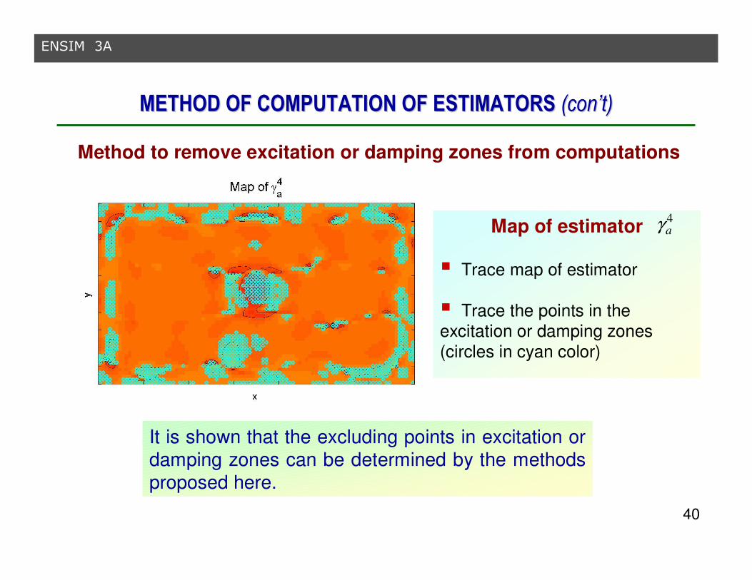
ENSIM 3A
Map of estimator
� Trace map of estimator
� Trace the points in the
excitation or damping zones
(circles in cyan color)
METHOD OF COMPUTATION OF ESTIMATORS METHOD OF COMPUTATION OF ESTIMATORS ((concon’’tt))
Method to remove excitation or damping zones from computations
4aγ
It is shown that the excluding points in excitation or
damping zones can be determined by the methods
proposed here.
41
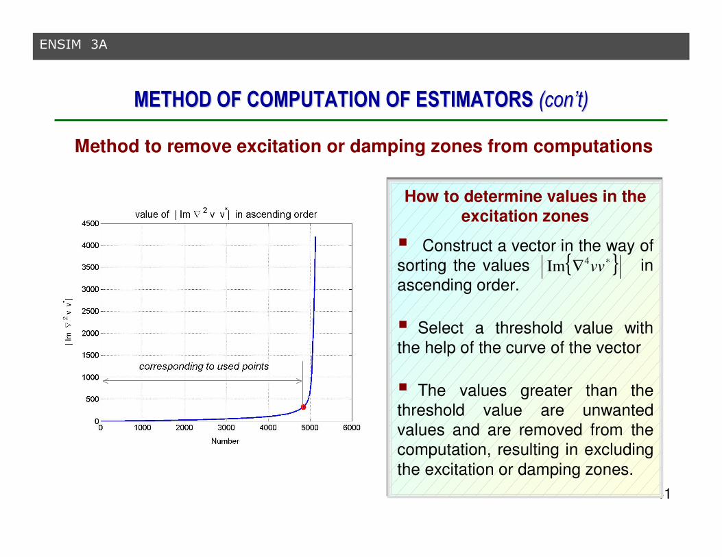
ENSIM 3A
How to determine values in the
excitation zones
� Construct a vector in the way of
sorting the values in
ascending order.
� Select a threshold value with
the help of the curve of the vector
� The values greater than the
threshold value are unwanted
values and are removed from the
computation, resulting in excluding
the excitation or damping zones.
METHOD OF COMPUTATION OF ESTIMATORS METHOD OF COMPUTATION OF ESTIMATORS ((concon’’tt))
Method to remove excitation or damping zones from computations
{ }∗∇ vv4
Im

42
ENSIM 3A
� The values are averaged over the
points selected using the histogram of � The values are averaged over the
points selected using the histogram of
METHOD OF COMPUTATION OF ESTIMATORS METHOD OF COMPUTATION OF ESTIMATORS ((concon’’tt))
ExamplesHistogram of at frequency indicatedaγ
aγbγ � The is computed
and shown by yellow band� The is computed
and shown by yellow band
42// bhD γωρ =
Experimental values have good agreement with Table values

43
ENSIM 3A
EXPERIMENTAL RESULTS OF EFFECTIVE PARAMETERS
Scanning Laser Vibrometer
� A scanning vibrometer use a OFV
300 optical head
� Two galvo-driven mirrors direct the
laser beam horizontally and vertically
� 32x32 measurement points
Structure for testing
�Test assembly consists of two steel plates
of thickness 1 mm
� The two opposite edges are clamped.
The two other edges are free
� A normal point force is acting on the plate
x
93
0
mm
850 mm
20 m
m
clampededge
free edge
y
Divergence of the structural intensity

44
ENSIM 3A
EXPERIMENTAL RESULTS OF EFFECTIVE PARAMETERS
The curve in dashed line is the wavenumber computed by
( ) 41eB Dhk ρω=
with
( )ω
ωγ
ρω
ωω
ω
ω
dh
Db
e ∫−=
2
1
4
2
12
1


