Laminar flow through Isotropic Granular Porous Media Sonia Woudberg Thesis presented in partial fulfilment of the requirements for the degree of Master of Engineering Science at the University of Stellenbosch. Promoter: Prof. J.P. du Plessis December 2006
Transcript
Laminar flow through Isotropic GranularPorous Media
Sonia Woudberg
Thesis presented in partial fulfilment of the requirements for the degree ofMaster of Engineering Science at the University of Stellenbosch.
Promoter: Prof. J.P. du Plessis
December 2006
Declaration
I, the undersigned, hereby declare that the work contained in this thesis is my own originalwork and that I have not previously in its entirety or in part submitted it at any universityfor a degree.
Signature: Date:
i
Abstract
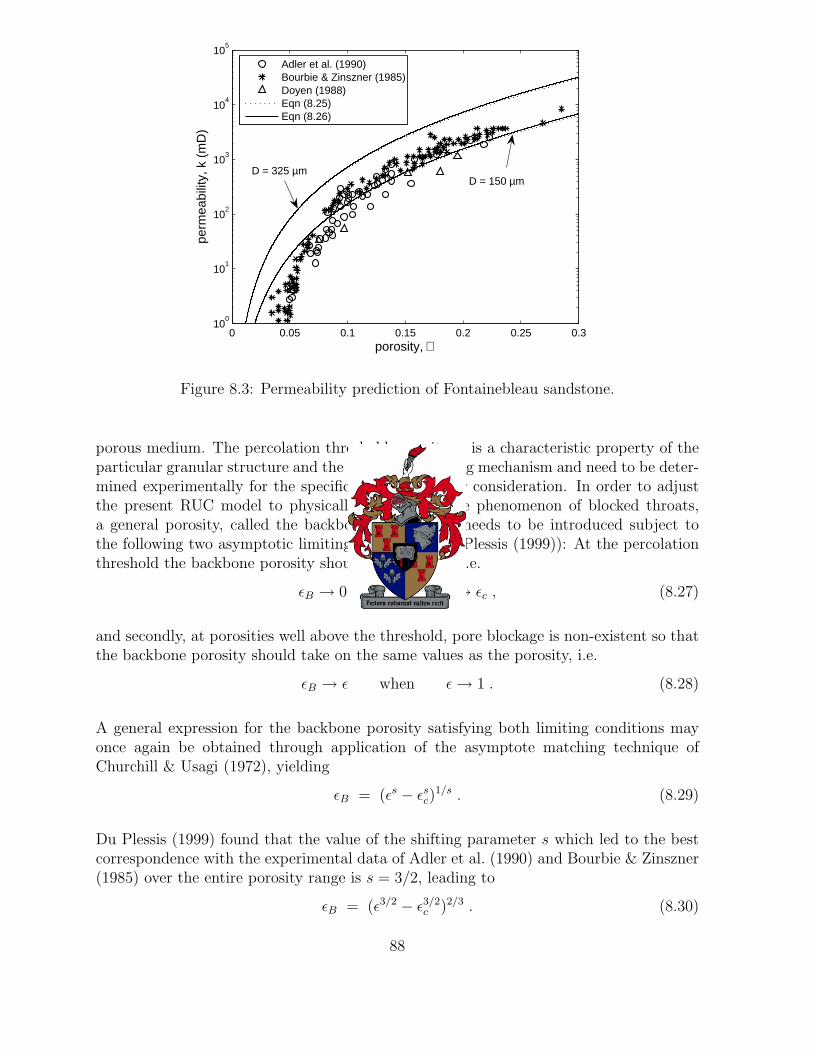
An analytical modelling procedure for predicting the streamwise pressure gradient forsteady laminar incompressible flow of a Newtonian fluid through homogeneous isotropicgranular porous media is introduced. The modelling strategy involves the spatial volumeaveraging of a statistical representative portion of the porous domain to obtain measurablemacroscopic quantities from which macroscopic transport equations can be derived. Asimple pore-scale model is introduced to approximate the actual complex granular porousmicrostructure through rectangular cubic geometry. The sound physical principles onwhich the modelling procedure is based avoid the need for redundant empirical coefficients.The model is generalized to predict the rheological flow behaviour of non-Newtonianpurely viscous power law fluids by introducing the dependence of the apparent viscosityon the shear rate through the wall shear stress. The field of application of the Newtonianmodel is extended to predict the flow behaviour in fluidized beds by adjusting the Darcyvelocity to incorporate the relative velocity of the solid phase. The Newtonian modelis furthermore adjusted to predict fluid flow through Fontainebleau sandstone by takinginto account the effect of blocked throats at very low porosities. The analytical model aswell as the model generalizations for extended applicability is verified through comparisonwith other analytical and semi-empirical models and a wide range of experimental datafrom the literature. The accuracy of the predictive analytical model reveals to be highlyacceptable for most engineering designs.
ii
Opsomming
’n Analitiese modelleringsprosedure is bekend gestel om die stroomsgewyse drukgradientvir tydonafhanklike, laminere, onsaamdrukbare vloei van ’n Newtoniese vloeistof deur ho-mogene, isotrope poreuse media met ’n korrelstruktuur te voorspel. Die modelleringstrate-gie berus op die ruimtelike volumetriese gemiddelde van ’n statisties-verteenwoordigendegedeelte van die poreuse medium om meetbare makroskopiese groothede te verkry waar-van makroskopiese oordragvergelykings afgelei kan word. ’n Eenvoudige porie-skaal modelword voorgestel om die werklike komplekse korrelagtige mikro-struktuur deur ’n reghoekigekubiese geometrie te benader. Die fisiese grondbeginsels waarop die modelleringstrategiegegrond is, vermy die behoefte vir empiriese koeffisiente. Die model is veralgemeen omdie reologiese vloeigedrag van nie-Newtoniese, suiwer viskeuse, magswet-vloeistowwe tevoorspel deur die afhanklikheid van die effektiewe viskositeit op die skuifspanningstempoin te voer deur die skuifspanning op die wand. The toepassingsveld van die Newtoniesemodel is uitgebrei om die vloeigedrag in sweefbeddens te voorspel deur die Darcy snel-heid aan te pas om sodoende die relatiewe snelheid van die vastestoffase in berekeningte bring. Die Newtoniese model is verder aangepas om die vloei van vloeistowwe deurFontainebleau sandsteen te voorspel deur die effek van geblokkeerde kanale by baie laeporositeite in ag te neem. Die analitiese model, sowel as die veralgemenings van diemodel vir uitgebreide toepasbaarheid, is geverifieer deur vergelyking met ander analitieseen semi-empiriese modelle en ’n wye verskeidenheid eksperimentele data vanuit die liter-atuur. Die akkuraatheid van die voorspelbare analitiese model blyk hoogs aanvaarbaarte wees vir die meeste ingenieursontwerpe.
iii
Acknowledgements
I wish to express my sincere gratitude to the following people who contributed to thisstudy by inspiring me in their own special way:
• God, for guiding me in life and giving me the potential to follow this path.
• My supervisor, Prof. Prieur du Plessis, for not only guiding me to face the challengesof our competitive world, but also showing me the world and to appreciate thepriceless things in life.
• My parents, Johann and Linda Woudberg, for the best moral and financial supportone could wish for.
• My sister and bother-in-law, Tania and Andre Heunis, for their concern and encour-agement.
• My family and friends for their wishes of support when I was overseas.
• Our head of division, Dr. Francois Smit, for his moral support at times when itmattered the most and the financial support from BIWUS to attend the conferencein India.
• Prof. Mark Knacksteadt for hosting me in Australia, Prof. Britt Halvorsen forhosting me in Norway and Prof. Jack Legrand for financial assistance to visitFrance.
• The South African National Research Foundation (NRF) for the Prestigious Scholar-ship and the additional Travel Grant.
E.2 Reynolds number and friction factor for power law flow through granularporous media . . . . . . . . . . . . . . . . . . . . . . . . . . . . . . . . . . 108
E.2.1 Reynolds number used by Smit (1997) . . . . . . . . . . . . . . . . 108
E.2.2 Reynolds number used by Smit & Du Plessis (2000) . . . . . . . . . 109
E.2.3 Friction factor used by Smit (1997) and Smit & Du Plessis (2000) . 109
viii
Nomenclature
Standard characters
a [m−1] specific surface
av [m−1] solid specific surface
A [] coefficient in the Blake-Kozeny equation
Ap [m2] cross-sectional flow area
B [] coefficient in the Burke-Plummer equation
d [m] linear dimension of RUC
dp [m] grain diameter
ds [m] linear dimension of solid cube in RUC
Dh [m] hydraulic diameter
Dp [m] spherical particle diameter
f [m−2] shear factor
fb [N.kg−1] external body forces per unit mass
F [ ] dimensionless shear factor
F [N ] drag force
g [N.kg−1] gravitational constant
k [m2] hydrodynamic or Darcy permeability
kkoz [ ] Kozeny constant
ko [ ] shape factor
K [N.s.m−2] consistency index of power law fluid
K [ ] dimensionless hydrodynamic permeability
l [m] length scale of microscopic structure
L [m] length scale of macroscopic structure
n [ ] behaviour index of power law fluid
n [ ] inwardly directed unit vector normal to surface of solid
ix
n [ ] unit vector in streamwise direction
p [Pa] interstitial pressure
q [m.s−1] superficial velocity, Darcy velocity or specific discharge
qmf
[m.s−1] minimum fluidization velocity
Q [m3.s−1] volumetric flow rate
ro [m] position vector of REV centroid
R [m] radius
Rh [m] hydraulic radius
Re [ ] pore Reynolds number (ρ q (d− ds)/µ)
Rec [ ] critical Reynolds number
Rep [ ] particle Reynolds number (ρ q ds/µ)
Sff [m2] fluid-fluid interfaces in REV
Sfs [m2] fluid-solid interface in RUC
Sfs [m2] fluid-solid interfaces in REV
Sg [m2] surface area in RUC adjacent to stagnant fluid volume
S|| [m2] surface area in RUC adjacent to streamwise fluid volume
S⊥ [m2] surface area in RUC adjacent to transverse fluid volume
Uf [m3] total fluid volume in RUC
Uf [m3] total fluid volume in REV
Ug [m3] total stagnant volume in RUC
Uo [m3] total (fluid and solid) volume of RUC
Uo [m3] total (fluid and solid) volume of REV
Us [m3] total solid volume in RUC
U s [m3] total solid volume in REV
Ut [m3] total transfer volume in RUC
U|| [m3] total streamwise volume in RUC
U⊥ [m3] total transverse volume in RUC
u [m.s−1] drift velocity
v [m.s−1] interstitial fluid velocity
w‖ [m.s−1] streamwise average pore velocity
w⊥ [m.s−1] transverse average pore velocity
x, y, z [m] distance along Cartesian coordinate
x
Greek symbols
β [ ] average pore velocity ratio
γ [s−1] shear rate
δ [ ] change in transverse property
∆ [ ] change in streamwise property
ǫ [ ] porosity
ǫB [ ] backbone porosity
ǫc [ ] percolation threshold porosity
ǫmf [ ] minimum fluidization porosity
η [N.s.m−2] apparent viscosity
Λ [s−1] dimensionless resistance factor
µ [N.s.m−2] fluid dynamic viscosity
ξ [ ] shear stress reduction coefficient
ρ [kg.m−3] fluid density
τ [N.m−2] local shear stress
τw [N.m−2] local wall shear stress
φ [ ] any tensorial fluid phase quantity
φs [ ] sphericity factor
Φsg [ ] total gas/particle drag coefficient
χ [ ] tortuosity factor
ψ [ ] geometric factor
Miscellaneous
∇ del operator
〈 〉 phase average operator
〈 〉f intrinsic phase average operator
{ } deviation operator
˜ interchange in unit vectors
vector (underlined)
diadic (doubly underlined)
xi
Acronyms
REV Representative Elementary Volume
RUC Representative Unit Cell
Subscripts
f fluid matter
fs fluid-solid interface
h hydraulic
o total solid- and fluid volume
s solid matter
w wall
|| parallel to streamwise direction
⊥ perpendicular to streamwise direction
0 lower limit
1 higher limit
xii
Chapter 1
Introduction
The term granular porous medium refers to a material consisting of an unconsolidatedsolid matrix with interconnected pores, as illustrated in Figure 1.1. One or several solid-and fluid phases may be involved. A porous medium is said to be permeable if it ispossible for the fluid phase to traverse through the interconnected pore sections. Theterm permeability is therefore used to describe the extent of conductance of fluid flowthrough the porous medium.
solid phase
fluid phase
Figure 1.1: A two-dimensional schematic representation of an unbounded granular porousmedium. The solid arrows indicate the direction of fluid flow through the pores.
A characteristic bulk property of a porous medium is the porosity ǫ which is defined as theratio of the void (which may be filled with liquid or gas) volume to the total (void and solid)volume of the porous medium. Granular porous media are classified as unconsolidatedmedia and occur either naturally or it is constructed commercially for various engineeringapplications. Examples are the natural phenomenon of fluid flow through granular soilssuch as sand, rock and sandstones and water seepage through the subsoil of dams andother construction materials. Sandstone is a natural porous rock formation of very low
1
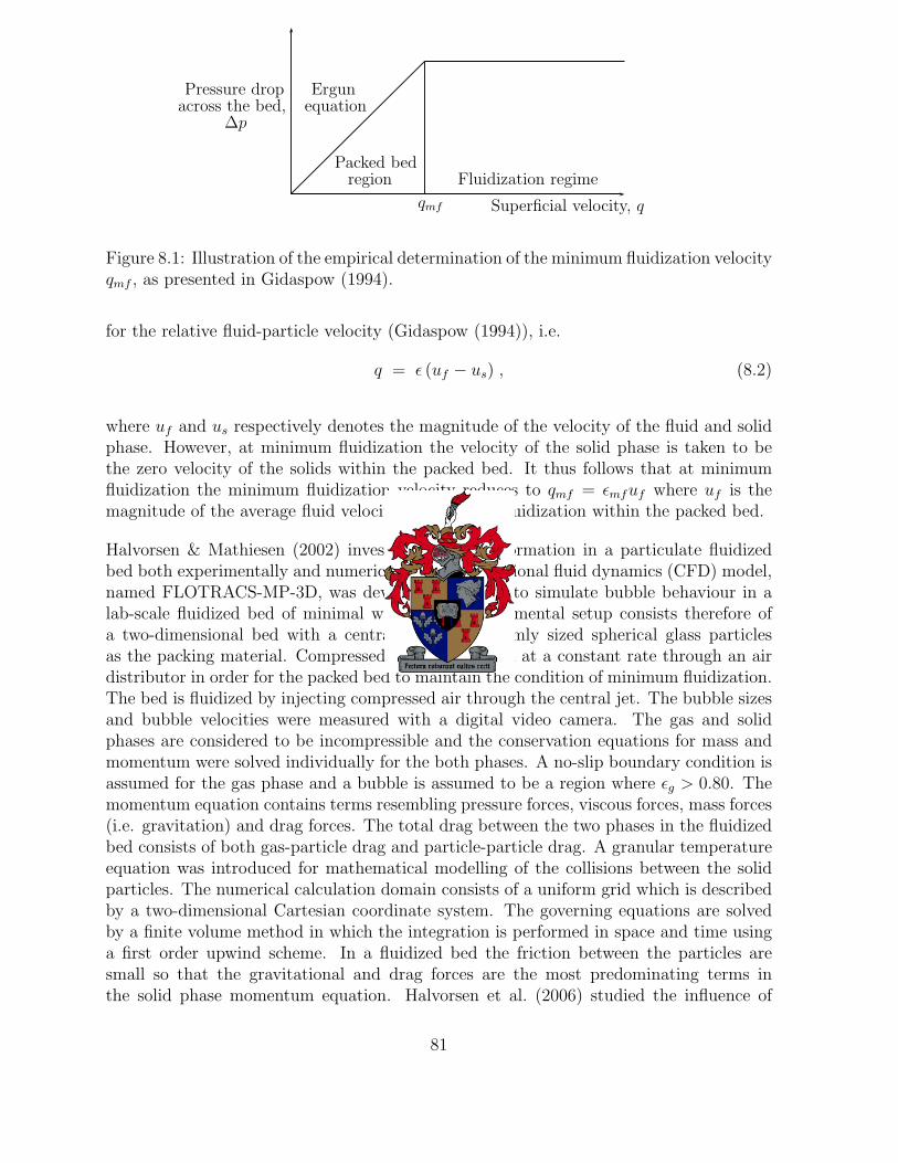
porosity (0.02 < ǫ < 0.35). Granular packed beds (0.25 ≤ ǫ ≤ 0.47) and fluidized beds(0.35 ≤ ǫ ≤ 0.8) are utilized for various applications in the chemical, pharmaceutical andpetroleum industries. Packed columns are widely used in fixed- and fluidized bed reactors,mass and heat transfer operations, separation processes and filtration.
Many years of research have been devoted to predicting the permeability of low to mod-erate porosity granular porous media. The ability to accurately predict the permeabilitythrough any type of granular porous medium, depends on a detailed description of thegranular microstructure. A thorough knowledge of the interstitial properties of the porousmedium is, however, an arduous task to obtain due to the complex geometry of the porousmatrix. As a result there are very few analytical models in the literature for predicting thepermeability through granular porous media. The customary procedure to follow recentlyis to solve the interstitial momentum transport equations through numerical simulations.Instead one seeks simple analytical techniques for predicting the permeability as a func-tion of the porosity without the need to obtain information on the complex interstitialproperties of the porous medium.
1.1 Granular models from literature
The methods for modelling flow through granular porous media found in the literaturemay be classified more or less into three categories, i.e. the capillary tube or hydraulicradius model, the submerged object model and models based on a statistical averagingapproach.
In the capillary tube or hydraulic radius approach the flow through a granular packed bedis regarded as being equivalent to flow through a network of capillary tubes of varyingcross-section but with a constant average cross-sectional area. The velocity profile isobtained by solving the Navier-Stokes equation for steady and fully developed flow. Anexpression is obtained for the pressure drop prediction across the packed bed.
Ergun (1952) proposed a semi-empirical capillary tube model for predicting the pressuredrop of a Newtonian fluid across a packed bed for Reynolds numbers ranging from thelaminar to the highly turbulent flow regimes. Despite many critical comments by manyauthors in the past (e.g. Dagan (1989) and Brea et al. (1976)) on the rather unrealisticcapillary representation of a packed bed, the Ergun equation proves to be somewhat moresuccessful than the submerged object models, based on the frequent use of the equation toserve as the onset of many other proposed models in the literature. The Ergun equationhas been modified by many authors (e.g. Gidaspow (1994), Yu et al. (1968) and Mishraet al. (1975)) to predict the flow behaviour in a fluidized bed. Mehta & Hawley (1969)modified the Ergun equation to take into account the effect of the column wall when thecolumn to particle diameter ratio is small. Bird et al. (2002) was the first to modifythe Ergun equation to describe the rheological flow behaviour of non-Newtonian fluids inporous media. The Ergun equation has also been modified extensively (Christopher &Middleman (1965), Kemblowski & Michniewics (1979), Brea et al. (1976)) to account for
2
non-Newtonian power law flow.
Macdonald et al. (1979) verified the predictive capabilities of the Ergun equation withexperimental data from the literature involving granular porous media of various porousmicrostructures and proposed different coefficient values for the Ergun equation.
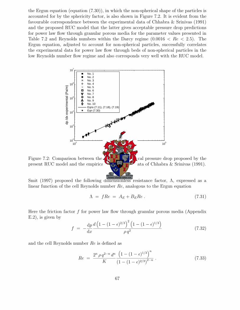
Sabiri & Comiti (1995) and Chhabra & Srinivas (1991) investigated the flowof a non-Newtonian purely viscous power law fluid through granular beds experimentallyand proposed an expression for predicting the pressure drop across the bed based on thecapillary tube model.
Chakrabarti et al. (1991) investigated the rheology of various concentrations of acommercial polymer solution through beds consisting of spherical particles experimentallyby using the capillary tube model.
The submerged object approach regards flow around an assemblage of submerged objectsforming a spatial array. The customary procedure to follow in determining the drag forceon a typical particle in the assemblage is by modification of the Stokes’ drag on a singleparticle to account for the additional resistance arising from the presence of neighbouringparticles.
Stokes’ flow (e.g. Chorlton (1967)) involves the steady creeping motion of an incom-pressible Newtonian fluid with a uniform approaching velocity past an isolated, stationarysphere embedded in a fluid of infinite extent. The drag force on the sphere is determinedby solving the Stokes equations.
Chester (1962) pointed out that when the Reynolds number is not negligibly smallStokes’ drag for flow past a sphere is inadequate since the inertial terms are not negligibleat great distance from the sphere. The drag force obtained from solving Oseen’s equationsprovides a first order expansion of the Reynolds number.
Hasimoto (1958) considered the steady motion of an incompressible Newtonian fluidpast a periodic array of small particles in a dilute medium. The drag force on a typicalsphere within the array was obtained by modification of the Stokes equations.
Happel (1958) proposed a concentric spherical cell model for predicting the flow of aNewtonian fluid through a random assemblage of spheres of low porosity in the creepingflow regime. The assemblage of spheres is regarded as a periodic array of identical sphericalcells. Each cell contains a single sphere surrounded by a fluid envelope with a frictionlessboundary. The Stokes’ equations subjected to appropriate boundary conditions weresolved and by application of Darcy’s law the pressure drop prediction across the bed wasobtained.
Various statistical averaging methods have been proposed in the literature, e.g. themethod involving a spatial volume averaging over a representative elementary volume,the method of homogenization for application to Stokes’ flow through periodic structuresand purely statistical averaging methods concerning probability density and uncertainty
3
distribution functions.
Dagan (1989) proposed a purely statistical model for predicting the permeability forsteady flow of an incompressible Newtonian fluid through a granular porous medium oflow porosity. The porous medium is regarded as a network of three-dimensional planarfissures with interconnected pores and identical constant apertures.
Du Plessis (1994) proposed an analytical model for predicting the pressure gradient forNewtonian flow through granular porous media for all porosities and Reynolds numbersranging from the Darcy regime to the steady laminar limit of the Forchheimer regime.The pore-scale model is based on a rectangular representation of the average granularporous microstructure.
Smit & Du Plessis (2000) extended the rectangular representative unit cell modelof Du Plessis & Masliyah (1991) to provide an analytical pressure drop prediction fornon-Newtonian purely viscous power law flow through porous media of various types ofporous microstructures, including granular media.
1.2 Objective
The capillary tube models are semi-empirical models in which empirical factors are intro-duced for correlation with experimental data. Many of the submerged object models, onthe contrary, are exact analytical models (e.g. the models of Stokes and Hasimoto) andtherefore lack the ability to be generalized for a broader field of application. Althoughthe capillary tube model have the ability to be extended for various other fields of appli-cability, its main draw back is its empiricism. Consequently, the need arises to producea simple generic analytical model of which the assumptions made within the analyticalmodelling procedure may easily be adapted to broaden its range of applicability.
Over the past two decades an analytical model has been developed at the University ofStellenbosch for predicting fluid flow through various types of porous media. The originalmodel was proposed in 1988 and has ever since been adapted to improve its predictivecapabilities. The objective of this work is to present the most recent improvement ofthe analytical model for predicting the pressure drop across a granular porous mediumfor Reynolds numbers within the steady laminar flow regime and over a wide range ofporosities.
4
1.3 Assumptions
In order to provide a relatively simple, but still realistic, pore-scale model to approximatethe complex geometry of the granular porous microstructure, some simplifying assump-tions need to be made.
This work concerns three-dimensional, isothermal, steady laminar flow of an incompress-ible viscous fluid through a granular porous medium. The porous medium is assumed tobe homogeneous and isotropic with respect to the average geometrical properties. Theporous medium is also assumed to be unbounded. Wall effects due to external boundariesmay therefore be neglected and as a result the local porosity may be assumed to be con-stant. The pore sections are assumed to be inter-connected, but may contain stagnantregions where the fluid remains stationary. The solid constituents are assumed to beuniformly sized, rigid, smooth and randomly distributed in all directions. The travers-ing fluid is assumed to consist of a single fluid phase, i.e. only saturated fluid flow isconsidered, with constant physical properties, unless otherwise stated. Both phases willbe treated as a continuum and therefore the terms ‘particle’ and ‘grain’ will be regardedas equivalent. It is furthermore assumed that the grains remain stationary, which maybe justified by the fact that in a packed bed the grains are supported by inter-particlecontact (Happel & Brenner (1965)).
1.4 Layout of thesis
The commencement of the analytical model to be introduced is the method of volumeaveraging of the transport equations describing the motion of the fluid through the porousmedium. The application of this method to the relevant transport equations is discussedin chapter 2. The granular pore-scale model is introduced in chapter 3 together with adiscussion of the laminar flow regimes under consideration. Chapters 4 and 5 are devotedto the analytical modelling of the pore-scale model within the two asymptotic limitingflow regimes discussed in chapter 4. The pore-scale model for Newtonian flow is presentedin chapter 6 and compared with the semi-empirical Ergun equation. The rest of this workconcerns generalizations of the Newtonian model. In chapter 7 the model is adaptedto account for non-Newtonian flow and in chapter 8 the Newtonian model is extendedfor application in fluidized beds and sandstones. Finally some conclusions are drawn inchapter 9.
5
Chapter 2
Method of Volume Averaging
This chapter concerns the local volume averaging of the momentum equations governingthe fluid transport within the pores of the porous medium. The method of volume av-eraging provides a manner of relating the interstitial flow conditions to the measurablemacroscopic flow behaviour.
2.1 Interstitial transport equations
The governing equations describing single phase flow of an incompressible Newtonian fluidin an infinitely permeable porous medium are the continuity equation for conservation ofmass, i.e.
∇ · v = 0 , (2.1)
and the Navier-Stokes equation for interstitial momentum transport derived from New-ton’s second law (e.g. Happel & Brenner (1965))
ρ∂ v
∂ t+ ∇ · (ρ v v) = −∇P + ∇ · τ + ρ f
b, (2.2)
where v is the interstitial fluid velocity at any point within the pore space, ρ is the constantfluid density, P is the interstitial hydrostatic pressure, τ is the local shear stress tensorof a Newtonian fluid and f
bdenotes the external body forces per unit mass. The terms
on the left hand side of equation (2.2) represent the time rate of change in momentumper unit volume of fluid, constituting the inertial forces, and the terms on the right handside represent the external forces per unit volume contributing to the nett force exertedon the differential fluid element. The external forces include body forces, e.g. gravitation,and pressure and viscous forces exerted on the surface of the fluid element. Assumingthat the gravitational force is a conservative force and discarding other external forces,f
bmay be expressed as f
b= −∇gz where z denotes an elevation and the gravitation
6
constant g is assumed to remain constant with variations in z. Under these conditions,the terms −∇P and ρf
bmay be combined to form a single term, i.e. −∇(P + ρ gz). For
relatively small values of z the gravitational term may be assumed to be negligible. Thepressure p = P + ρ gz will henceforth be referred to as the interstitial dynamic pressure.The Navier-Stokes equation may accordingly be expressed as
ρ∂ v
∂ t+ ∇ · (ρ v v) = −∇p + ∇ · τ , (2.3)
The method of volume averaging over a representative portion of the fluid domain to ob-tain local measurable macroscopic volume averaged transport equations has been studiedby many authors (e.g. Bear & Bachmat (1986), Slattery (1969) and Whitaker (1969)).The next section will shortly address some of the basic principles on which the method isbased.
2.2 Representative Elementary Volume
A Representative Elementary Volume, abbreviated REV, is defined as an averaging vol-ume Uo of finite extent within the porous domain (e.g. Whitaker (1999)), consistingof both fluid and solid phases, respectively denoted by Uf and U s. A two-dimensionalschematic representation of a spherical REV is shown in Figure 2.1.
U s
Uf
Sff
Sfs
O
ro
L
l
Figure 2.1: A two-dimensional schematic representation of a spherical REV. The dashedline indicates the REV boundary.
An REV is defined at each an every point within the unbounded porous medium. Thecentroid of each REV is indicated by a position vector ro relative to some arbitrary origin
7
O, as illustrated in Figure 2.1 for a single REV. Inter-connectivity of the pore space andtreating the fluid phase as a continuum are essential requirements for an REV. Althoughthe shape of the REV is not prescribed, it should ensure that the averaging functionsare continuous and also continuously differentiable to any order. It is however requiredthat the size, shape and orientation of the REV should remain constant. The REV ischosen to be the smallest possible volume containing sufficient fluid and solid parts to bestatistically representative of the local average properties, e.g. the local porosity. Thesize of the REV is appropriately chosen when small variations in the local volume willnot change the values of the local average properties. In terms of the linear dimensionsindicated in Figure 2.1, this will require that l >> dp and l << L. The fluid-solidinterfaces within the REV are denoted by Sfs and the fluid-fluid interfaces on the REVboundary by Sff . The porosity ǫ of the REV is assumed to be uniform and constant andis defined by the volumetric ratio
ǫ ≡ Uf
Uo
. (2.4)
2.3 Macroscopic volume averaged quantities
The concept of an REV leads to the introduction of various measurable macroscopicvolume averaged quantities. The superficial velocity q, also known as the Darcy velocityor specific discharge, is defined as the phase average (Appendix A.1) of the interstitialfluid velocity v, i.e.
q = 〈 v 〉 =1
Uo
∫∫∫
Uf
v dU , (2.5)
and represents the average velocity that would prevail in a section of the porous mediumin which no solid phase is present. For this reason it is customary to use the superficialvelocity in the comparison of different flow systems. The streamwise direction n is definedas the direction of the superficial velocity, that is
n = q/q . (2.6)
The drift velocity u is defined as the intrinsic phase average (Appendix A.1) of the inter-stitial velocity v, i.e.
u = 〈 v 〉f =1
Uf
∫∫∫
Uf
v dU , (2.7)
and represents the average fluid velocity in the streamwise direction. The relationshipbetween the superficial- and drift velocity is given by
q = ǫ u , (2.8)
8
which is known as the Dupuit-Forchheimer relation. The deviation of any fluid phasetensorial quantity φ at any point within Uf is denoted by {φ} and defined as
{φ} ≡ φ − 〈φ〉f . (2.9)
2.4 Macroscopic transport equations
Volume averaging of the continuity equation for an incompressible fluid over a sufficientlylarge REV (Appendix A.2) leads to
∇ · q = 0 , (2.10)
and the volume averaged Navier-Stokes equation (Appendix A.3) for an incompressiblefluid may be expressed as
−∇〈 p 〉 = ρ∂ q
∂ t+ ρ∇ ·
(q q/ǫ
)+ ρ∇ · 〈{v} {v}〉 − ∇ ·
⟨τ⟩
+1
Uo
∫∫
Sfs
(n {p} − n · τ
)dS . (2.11)
where n is the inwardly directed unit vector normal to the surface of the solid and 〈 p 〉 de-notes the average macroscopic pressure. Equation (2.11) predicts the streamwise pressuregradient for unidirectional average flow over any type of porous medium, e.g. granularmedia, foams and fibre beds. The surface integral contains all the information on the fluid-solid interaction and depends strongly on the porous microstructure. The evaluation ofthe surface integral is subjected to a detailed and accurate description of the interstitialpressure- and velocity gradients at the fluid-solid interfaces. In order to circumvent thecomplex geometry of the solid constituents, a pore-scale model resembling the porousmicrostructure will be introduced in the following chapter to approximate and quantifythe surface integral for the particular case of a granular porous medium.
9
Chapter 3
Rectangular Granular Pore-ScaleModel
This chapter introduces the concept of a pore-scale model for closure modelling of theinterstitial fluid-solid interaction to analytically quantify the pressure gradient predictionover a granular porous medium.
3.1 Rectangular Representative Unit Cell
A rectangular Representative Unit Cell, abbreviated RUC, was originally introduced byDu Plessis & Masliyah (1988) for isotropic sponge-like media. A rectangular RUC isdefined as the smallest rectangular control volume, Uo, into which the local average prop-erties of the REV may be embedded. The granular RUC model was introduced by DuPlessis & Masliyah (1991) after which some of the model assumptions were improved byDu Plessis (1994). The latter model will henceforth be referred to as the existing RUCmodel. The granular RUC model is schematically illustrated in Figure 3.1. The fluid filledvolume within the RUC is denoted by Uf and Us denotes the volume of the solid phase.The RUC is assumed to be homogeneous and isotropic in accordance with the averagegeometry of the porous medium. The assumption of average geometrical isotropy allowsthe introduction of a cubic RUC of linear dimension d, defined as the average lengthscale over which similar changes in geometrical and physical properties take place. Thesolid cube represents the average geometric properties of the granular solid microstruc-ture. The length of the cube is denoted by ds. The cubic geometry of the RUC model isintroduced for mathematical simplicity and serves as an approximation for flow throughan assemblage of grains with arbitrary shape. The solid cube is assumed to be stationaryand is positioned so that a vector normal to any of the cube’s faces is parallel to a normalvector on the corresponding face of the RUC. Due to the parallel alignment of the solidcubes’ faces with that of the RUC, one of the fluid channels will always be aligned withthe streamwise direction, leaving the remaining two channels to be directed in transverse
10
d
d
d
Us
Uf
ds
ds
ds
n
Figure 3.1: Cubic geometry of the RUC model for modelling the fluid flow through anisotropic granular porous medium. The streamwise direction is indicated by n.
directions, that means, directions perpendicular to the streamwise direction. Any propertyreferring to the streamwise direction will henceforth be denoted by a subscript ‖ and anyproperty related to a transverse direction by ⊥. The porosity ǫ of the RUC is assumed tobe equivalent to the porosity of the REV and is defined as
ǫ =Uf
Uo
. (3.1)
The fluid filled volume Uf and the volume of the solid cube Us may be expressed in termsof the linear dimensions d and ds as follows
Uf = ǫ Uo = ǫ d3 , (3.2)
Us = d3s , (3.3)
which lead to the following relationship between the linear dimensions of the RUC interms of the porosity ǫ:
ds = (1 − ǫ)1
3 d . (3.4)
3.2 Staggered and non-staggered arrays
The relative transverse positioning of neighbouring RUC’s in the streamwise directionleads to the introduction of two arrays yielding different fluid flow phenomena. The arrayin which maximum possible staggering of the solid cubes in a straight streamtube of widthd occurs in the streamwise direction, is referred to as a fully staggered array and the arrayin which no staggering occurs in any of the three principal directions, is referred to as a
11
regular array. This section forms an extension of the existing RUC model since the lattermodel did not consider an array in which splitting of the stream-tube occurs neither onein which stagnant regions are present.
3.2.1 Fully staggered array
A typical two-dimensional RUC within a streamwisely fully staggered array is schemati-cally illustrated in Figure 3.2.
n
Figure 3.2: A two-dimensional schematic representation of a fully staggered array. Theboundaries of a typical RUC is indicated by the bold dashed lines and the dotted linesrepresent a stream-tube.
In a fully staggered array the streamwise flux is split and then deviated in oppositetransverse directions to traverse past the solid cube opposing the motion of the fluidin the streamwise direction. The streamwise flux reunites on the lee side of this cubeand proceeds to flow in the streamwise direction before the next solid obstacle causesthe streamwise flux to split again and the process repeats itself. A fully staggered arraycontains no stagnant regions and no staggering occurs in the two transverse directions.Also shown in Figure 3.2 is a stream-tube, represented by the dotted lines, that servesas a fluid envelope through which the fluid flows in the streamwise direction. Since thestream-tube consists of a bundle of streamlines which may not cross, it is assumed thatall the fluid enters the RUC through the upstream face and exits through the downstreamface with no fluid exchange across the transverse facing surfaces of the RUC. Figure 3.3is a three-dimensional schematic representation of an RUC within a fully staggered array.
12
n
d
ds Us
ds
2
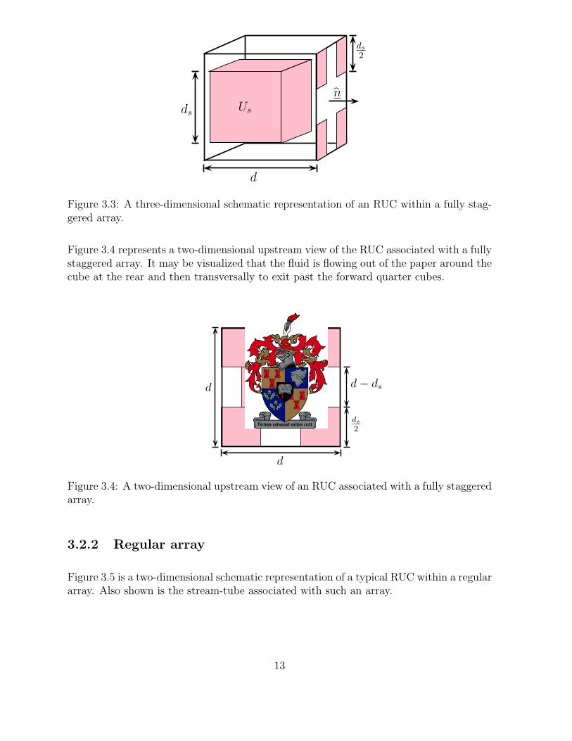
Figure 3.3: A three-dimensional schematic representation of an RUC within a fully stag-gered array.
Figure 3.4 represents a two-dimensional upstream view of the RUC associated with a fullystaggered array. It may be visualized that the fluid is flowing out of the paper around thecube at the rear and then transversally to exit past the forward quarter cubes.
d
d
ds
2
d− ds
Figure 3.4: A two-dimensional upstream view of an RUC associated with a fully staggeredarray.
3.2.2 Regular array
Figure 3.5 is a two-dimensional schematic representation of a typical RUC within a regulararray. Also shown is the stream-tube associated with such an array.
13
n
Figure 3.5: A two-dimensional schematic representation of a regular array. The bound-aries of a typical RUC is indicated by the bold dashed lines and the dotted lines representa stream-tube.
In a regular array the fluid enters and leaves the RUC in the streamwise direction withoutbeing deviated in a transverse direction, that is, in a regular array no staggering occurs.A regular array contains stagnant regions where the fluid remains stationary betweenany two neighbouring cubes in the streamwise direction. Note that in each of the threeprincipal directions normal to the cube faces no staggering occurs. A three-dimensionalschematic representation of an RUC within a regular array is shown in Figure 3.6.
d
ds Us
n
Figure 3.6: A three-dimensional schematic representation of an RUC within a regulararray.
Figure 3.7 shows a two-dimensional upstream view of a regular array. The fluid may bevisualized to be flowing out of the paper, past the cubes which are positioned directlybehind each other in the streamwise direction.
14
d
d
ds
d− ds
Figure 3.7: A two-dimensional upstream view of an RUC associated with a regular array.
3.3 Piece-wise straight streamlines
The adopted rectangular geometry and the isotropy requirement of the RUC model allowfor the facing surfaces of any two neighbouring cubes to be a uniform distance d − ds
apart, yielding pair-wise sets of equal parallel plates. In conjunction with the parallelplate configuration, piece-wise straight streamlines, between and parallel to the plates,are assumed to prevail within all the flow channels, as illustrated in Figure 3.8 for therespective arrays.
n
(a) Fully staggered array (b) Regular array
Figure 3.8: A two-dimensional representation of the piece-wise straight streamlines asso-ciated with (a) a fully staggered array and (b) a regular array. The dashed lines representthe streamlines and the bold dashed lines a typical RUC.
The splitting of the stream-tube into two equal but directionally opposite transverse fluidvolumes within a fully staggered array is clearly illustrated by the streamlines in Figure3.8 (a). Figure 3.8 (b) shows the stagnant volume, indicated by the absence of streamlines,present between any two neighbouring cubes in the streamwise direction within a regulararray.
15
3.4 Volume partitioning
The piece-wise straight streamlines allow for the fluid domain within an RUC to bepartitioned into different sub-volumes depending on the orientation of the particular fluidvolume with respect to the streamwise direction and the presence of surfaces adjacent tothe specific fluid volume under consideration. The concept of volume partitioning of thefluid domain was not considered in the existing RUC model. The volume partitioning ofthe fluid domain within the RUC presented in Figure 3.6 for a regular array is shown inFigure 3.9. As opposed to the other figures shown thus far, the shaded volumes withinFigure 3.9 represent fluid volumes. The solid volumes are not shown.
n
Ut
n
UgSg
U‖
U‖
S‖
Figure 3.9: A three-dimensional volume partitioning of the fluid domain within the RUCpresented in Figure 3.6 for a regular array. The shaded volumes represent fluid volumes,solid volumes are not shown.
The fluid volume in the channels parallel to the streamwise direction and adjacent tosolid surfaces is denoted by U‖ and is referred to as a streamwise volume. The solidsurfaces adjacent to U‖ are denoted by S‖ and are referred to as the streamwise surfaces.The fluid volume in the stagnant regions between any two neighbouring cubes in thestreamwise direction, is denoted by Ug and is referred to as a stagnant volume. The solidsurfaces adjacent to Ug are denoted by Sg and are referred to as the stagnant surfaces.The fluid volume involving no shear stresses due to the absence of adjacent solid surfacesis denoted by Ut and is referred to as a transfer volume. Similarly, volume partitioningmay be applied to the fluid domain within the RUC presented in Figure 3.3 for a fullystaggered array. The volume partitioning of a fully staggered array is not shown becauseof the complexity of illustrating it graphically. As opposed to the stagnant region withina regular array, a fully staggered array is characterized by a fluid volume in which thefluid flows in directions perpendicular to the streamwise direction. These fluid volumes,denoted by U⊥, are adjacent to solid surfaces and are referred to as the transverse volumes.The solid surfaces adjacent to U⊥ are denoted by S⊥ and are referred to as the transversesurfaces. The total fluid volume Uf contained within an RUC associated with any of thetwo arrays may thus be expressed as
Uf = U‖ + U⊥ + Ug + Ut , (3.5)
16
and the total fluid-solid interfaces Sfs may accordingly be expressed as
Sfs = S‖ + S⊥ + Sg . (3.6)
For a fully staggered array Ug = Sg = 0 and for a regular array U⊥ = S⊥ = 0. Theexpressions for the three-dimensional surface- and volume partitioning of the respectivearrays are presented in Table 3.1 in terms of the linear dimensions d and ds. The expres-sions presented in Table 3.1 denote the total volume (or surface area) associated with thespecified volume (or surface).
Array
Parameter Fully staggered Regular
Uo d3
Us d3s
Uf d3 − d3s
Ut (d− ds)2 (d+ 2ds)
U‖ 2 d2s(d− ds)
S‖ 4 d2s
U⊥ d2s(d− ds) 0
S⊥ 2 d2s 0
Ug 0 d2s(d− ds)
Sg 0 2 d2s
Table 3.1: Three-dimensional surface- and volume partitioning for the RUC’s associatedwith a fully staggered- and regular array.
The volume partitioning of the fluid domain allows for the introduction of a streamwiseaverage pore velocity w‖ (Du Plessis (1994)), defined as
w‖ =1
U‖ + Ut
∫∫∫
Uf
v dU (3.7)
and relates as follows to the superficial velocity q,
w‖ =q d2
Ap‖
, (3.8)
17
where Ap‖ is the streamwise cross-sectional flow area available for fluid discharge throughthe RUC, i.e.
Ap‖ = d2 − d2s . (3.9)
It thus follows that
w‖ =q d2
d2 − d2s
. (3.10)
As listed in Table 3.1, different expressions are obtained for U‖ and U⊥ implying that theaverage pore velocities within these two fluid volumes should differ. A coefficient β istherefore introduced to account for the different average velocities in the streamwise andtransverse channels and is defined as
β ≡ w⊥
w‖
, (3.11)
with w⊥ the magnitude of the transverse average pore velocity. A geometric factor ψ,defined as
ψ =Uf
U‖ + Ut
=U‖ + Ut + U⊥ + Ug
U‖ + Ut
, (3.12)
was introduced by Lloyd et al. (2004). This factor yields the same result for a both afully staggered- and non-staggered array, i.e.
ψ =ǫ
(1 − (1 − ǫ)2/3). (3.13)
The reason for the introduction of the geometric factor ψ will be addressed in the followingchapter.
3.5 Volume averaging of transport equations over an
RUC
Volume averaging of the Navier-Stokes equation for incompressible flow over a typicalRUC may be expressed as
−∇〈p〉 = ρ∂ q
∂ t+ ρ∇ ·
(q q/ǫ
)+ ρ∇ · 〈{v} {v}〉 − ∇ ·
⟨τ⟩
+1
Uo
∫∫
Sfs
(n {p} − n · τ
)dS , (3.14)
where n denotes the inwardly directed unit vector normal to one of the cube faces. To-gether with the volume averaged continuity equation of an incompressible fluid, that is,
∇ · q = 0 , (3.15)
18
these equations describe the fluid transport through an RUC, which represents the aver-age geometric and physical properties of the granular porous medium. Equation (3.14)provides an expression for the streamwise pressure gradient over the linear dimension dof the RUC. The momentum dispersion term, ρ∇ · 〈{v}{v}〉, may be expressed as followsin terms of the superficial velocity q (Appendix A.3):
ρ∇ · 〈{v}{v}〉 = ρ∇ ·⟨q q⟩− 2
ǫρ∇ ·
⟨q q⟩
+1
ǫ2ρ∇ ·
⟨q q⟩, (3.16)
It thus follows that
−∇〈p〉 = ρ∂ q
∂ t+ ρ∇ ·
(q q/ǫ
)+ ρ∇ ·
⟨q q⟩− 2
ǫρ∇ ·
⟨q q⟩
+1
ǫ2ρ∇ ·
⟨q q⟩
− ∇ ·⟨τ⟩
+1
Uo
∫∫
Sfs
(n {p} − n · τ
)dS . (3.17)
For a Newtonian fluid of constant viscosity µ, it follows that ∇ ·⟨τ⟩
= µ∇2q, yielding
−∇〈p〉 = ρ∂ q
∂ t+ ρ∇ ·
(q q/ǫ
)+ ρ∇ ·
⟨q q⟩− 2
ǫρ∇ ·
⟨q q⟩
+1
ǫ2ρ∇ ·
⟨q q⟩
− µ∇2q +1
Uo
∫∫
Sfs
(n {p} − n · τ
)dS . (3.18)
All the terms in equation (3.18), except the surface integral, are macroscopic terms. Theterm −µ∇2q represents the macroscopic viscous shear at external walls, which may be ne-glected since the porous medium is assumed to be unbounded. Justified by approximatedexperimental conditions (Dybbs & Edwards (1982)), a uniform superficial velocity field qmay be assumed. Since a uniform average velocity field implies macroscopic conservationof momentum, all the terms resulting from the interstitial rate of change in momentumshould vanish macroscopically, which is indeed the case when q is assumed to be uni-form in equation (3.18). It thus follows that for steady flow of an incompressible viscousfluid through a homogeneous porous medium in which a uniform average velocity field isassumed, the streamwise pressure gradient may be expressed as
−∇〈p〉 =1
Uo
∫∫
Sfs
(n p− n · τ
)dS . (3.19)
Equation (3.19) represents a force balance between the external pressure gradient for fluidtransport through the RUC and the pressure and viscous forces exerted by the solid cubeon the traversing fluid. The first term in the surface integral denotes the inertial pressureforces exerted by the solid cube on the traversing fluid due to a pressure variation overthe upstream and downstream facing surfaces of the cube. The pressure variation results
19
from a change in momentum across the streamwise facing surfaces of the cube. Notethat these inertial pressure forces are interstitial forces which contribute to the externalpressure gradient, as opposed to the macroscopic inertial forces that vanished due to theassumption of a uniform average velocity field. Interstitially changes in momentum occur,which become significant at higher Reynolds numbers, but macroscopically momentum isconserved. The second term in the surface integral denotes the viscous forces exerted bythe solid cube on the traversing fluid due to shear stresses at the fluid-solid interfaces.Since the Reynolds number is defined as the ratio of the inertial forces to the viscousforces, the contribution of the pressure- and viscous forces to the streamwise pressuregradient depends on the magnitude of the Reynolds number. The Reynolds number usedin the RUC model is a particle Reynolds number Rep, defined in terms of the length ds
of the solid cube, i.e.
Rep =ρ q ds
µ. (3.20)
The following chapters concern closure modelling of the surface integral of equation (3.19)in order to analytically quantify the fluid-solid interaction in the limit of very low Reynoldsnumber flow and in the steady laminar limit of the inertial flow regime to obtain a generalexpression for the streamwise pressure gradient over a wide range of Reynolds numbersthrough application of an asymptote matching technique.
3.6 Classification of laminar flow regimes
Three laminar flow regimes will be considered, namely the asymptotic limit of low Reynoldsnumber flow in the Darcy or creeping flow regime, the steady laminar limit of the inertialor Forchheimer flow regime and the transition regime in between which is characterized bythe development of boundary layers. The steady laminar limit is followed by an unsteadylaminar flow regime and at even higher Reynolds numbers the boundary layer becomesturbulent (Dybbs & Edwards (1982)). Since only steady flow is considered, the latter tworegimes fall beyond the scope of this work.
3.6.1 Limit of low Reynolds number flow
The Darcy or creeping flow regime corresponds to a pore Reynolds number Re < 1 (Dybbs& Edwards (1982)). The analytical modelling procedure of the RUC model in this regimewill concern pore Reynolds numbers within the asymptotic limit, i.e. Re ≈ 0.1. Theanalogue between the streamlines associated with flow past a sphere and a cube in thelimit of low Reynolds number flow is schematically shown in Figure 3.10. The piece-wisestraight streamlines assumed by the RUC model for flow past a cube is clearly illustrated.
20
Flow past a sphere (Re ≈ 0.1) Flow past a cube (Re ≈ 0.1)
Figure 3.10: A two-dimensional schematic representation of the streamlines associatedwith flow past a sphere and a cube in the limit of low Reynolds number flow.
In this limit the viscous forces predominate over the inertial pressure forces and con-sequently the flow pattern is strongly influenced by the granular microstructure. Theadvantage of modelling fluid flow through the pores within this limit is that a fully de-veloped velocity profile may be assumed to prevail throughout all the pore sections. Theentrance effects arising from the gradual build-up of a developing velocity profile maythus be neglected.
3.6.2 Transition regime
The transition from the Darcy to the Forchheimer regime is due to the development ofboundary layers near the solid surfaces within the pores. This regime is associated with1 < Re < 100 (Dybbs & Edwards (1982)). In the transition regime both the inertial andviscous forces contribute to the streamwise pressure gradient. The flow conditions in thisregime are not modelled explicitly as it would require an enormous computational effort.The applied asymptote matching is assumed to be reasonably accurate in predicting thetransitional effects.
3.6.3 Steady laminar limit of the inertial flow regime
The steady laminar limit of the inertial flow regime corresponds to Re > 100 (Dybbs &Edwards (1982)). At Reynolds numbers just before the commencement of the inertialflow regime, the boundary layer begins to separate from the downstream stagnation pointon the lee side of the solids grains. The boundary layer moves further downstream as theReynolds number increases until the steady laminar limit is reached at which a separationzone is formed on lee side of the solids grains. The analogue between the separation zonefor flow past a sphere and a cube within the steady laminar limit of the inertial flowregime is schematically illustrated in Figure 3.11.
21
Flow past a sphere (Re > 100) Flow past a cube (Re > 100)
Figure 3.11: A two-dimensional schematic representation of the streamlines associatedwith flow past a sphere and a cube in the steady laminar limit of the inertial flow regime.
In the separation zone a low fluid velocity persists whereas, on the boundary of theseparation zone, the fluid velocity is relatively high. As a result of the significant differencein flow velocities an interstitial recirculation pattern is generated within the separationzone. The entire square surface on the lee side of the solid is therefore exposed to arelatively low pressure. The resulting streamwise pressure difference between the upstreamand downstream facing surfaces of the solid grains depends on the size of the separationzone which, in turn, depends on the position of the point of separation. The pointof separation is again determined by the shape or form of the solid obstacle. This isthe reason why the pressure force resulting from the pressure difference across a singleisolated solid grain is referred to in the literature as form drag. For a laminar boundarylayer separation occurs about midway between the front and rear of the solid (Roberson& Crowe (1985)). As a result of the separation of the boundary layer from the surfaceof the solid, the surface area on which the shear stresses act, is diminished substantially.Consequently, in the steady laminar limit of the inertial flow regime the pressure forcespredominate over the viscous shear forces.
22
Chapter 4
Low Reynolds Number Flow Regime
This chapter involves the analytical closure modelling of the fluid-solid interaction withinthe RUC for predicting the streamwise pressure gradient in the asymptotic limit of lowReynolds number flow.
4.1 Closure modelling at low to moderate porosities
The assumption of flow between parallel plates is only valid for low to moderate porositieswhere neighbouring cubes are present. At high porosities neighbouring cubes are absent sothat the parallel plate configuration no longer persists and the assumption of flow betweenparallel plates is no longer valid. The RUC model within the limit of low Reynolds numberflow will therefore be classified as a low to moderate porosity model (i.e. ǫ < 0.8). Fullydeveloped laminar flow of a Newtonian fluid is assumed to prevail piece-wise throughoutall pore sections. The closure modelling procedure with the three-dimensional granularRUC model to be presented in this work closely follows the work of Lloyd et al. (2004)for two-dimensional Newtonian flow perpendicular to a unidirectional fibre bed, althoughsome discrepancies occur (Appendix B). The streamwise pressure gradient resulting fromvolume averaging of the transport equations in which a uniform velocity field q is assumed(Chapter 3), is given by
−∇〈p〉 =1
Uo
∫∫
Sfs
(n p− n · τ
)dS . (4.1)
It was established by Lloyd (2003) that for low porosity media in the creeping flow regimethe pressure term in the surface integral of equation (4.1) contains a viscous effect whichcontributes significantly to the streamwise pressure gradient. Although the viscous forcespredominate over the inertial pressure forces in this regime, the pressure term should notbe neglected. The shear stresses on the surfaces within the transverse channels are accom-panied by transverse pressure gradients. These pressure gradients are contained within
23
the pressure term in the surface integral of equation (4.1). The commencement of theclosure modelling procedure is the evaluation of the surface integral over the streamwise-,transverse- and stagnant surfaces within and adjacent to the RUC, yielding
−∇〈p〉 =1
Uo
∫∫
S‖
n p dS +1
Uo
∫∫
S⊥ + Sg
n p dS − 1
Uo
∫∫
S‖
n · τ dS
− 1
Uo
∫∫
S⊥
n · τ dS − 1
Uo
∫∫
Sg
n · τ dS . (4.2)
The parallel alignment of the streamwise surfaces of neighbouring cubes in the transversedirections results in a vectorial cancelation of the pressure on the streamwise surfaces,that is,
1
Uo
∫∫
S‖
n p dS = 0 . (4.3)
Although streamlines may appear in the stagnant volume Ug of a regular array, the corre-sponding velocities will be very small (Lloyd (2003)). Assuming therefore that the shearstresses on Sg are negligible, it follows that
1
Uo
∫∫
Sg
n · τ dS = 0 . (4.4)
Equation (4.2) there-upon simplifies to
−∇〈p〉 =1
Uo
∫∫
S⊥ + Sg
n p dS − 1
Uo
∫∫
S⊥
n · τ dS − 1
Uo
∫∫
S‖
n · τ dS . (4.5)
The quasi-periodic structure of the RUC model in the streamwise direction, i.e. eachupward transverse channel is to be followed by an opposite downward transverse channel,plays an important role in the further analysis of the remaining surface integrals regardingthe particular location of the RUC in the streamwise direction. It is therefore of utmostimportance that all possible locations of the RUC in the streamwise direction should beconsidered. The two typical choices of RUC’s chosen to accomplish the latter requirementare illustrated in Figures 4.1 and 4.2 for a fully staggered- and regular array, respectively.The upstream and downstream facing surfaces of the RUC with corner points AAAA cutthrough solid parts and the upstream and downstream facing surfaces of the RUC withcorner points BBBB do not cut through any solid parts. S⊥AA and S⊥BB respectivelydenotes the fluid-solid interfaces adjacent to U⊥ of the RUC with corner points AAAAand BBBB in the fully staggered array shown in Figure 4.1. Similarly, SgAA and SgBB
respectively denotes the fluid-solid interfaces adjacent to Ug of the RUC with corner pointsAAAA and BBBB in the regular array shown in Figure 4.2.
24
n
U⊥
U⊥
U⊥
U⊥
A AB B
A B A B
Figure 4.1: Schematic illustration of the two typical choices of RUC’s in a fully staggeredarray to consider all possible locations in the streamwise direction.
A A
A A
B B
B B
n
Ug Ug
Figure 4.2: Schematic illustration of the two typical choices of RUC’s in a regular arrayto consider all possible locations in the streamwise direction.
The relative frequency of occurrence of the RUC with corner points AAAA in the stream-wise direction is ds/d and the relative frequency of occurrence of the RUC with cornerpoints BBBB in the streamwise direction is (d − ds)/d. If the transverse and stagnantsurface integrals of equation (4.5) are weighed according to these relative frequencies ofoccurrence, over a streamwise displacement d, it follows that
−∇〈p〉 =ds
d· 1
Uo
∫∫
S⊥AA + SgAA
n p dS +d− ds
d· 1
Uo
∫∫
S⊥BB + SgBB
n p dS
− ds
d· 1
Uo
∫∫
S⊥AA
n · τ dS − d− ds
d· 1
Uo
∫∫
S⊥BB
n · τ dS − 1
Uo
∫∫
S‖
n · τ dS . (4.6)
Assuming that the pressure p on all facing pairs of transverse and stagnant surfaces are
25
equal, results in a vectorial cancelation of the pressures on these surfaces, that is
ds
d· 1
Uo
∫∫
S⊥AA + SgAA
n p dS = 0 . (4.7)
The RUC with corner points BBBB in the fully staggered array contains two transversechannels in which the fluid flows in opposite directions perpendicular to the streamwisedirection. The shear stresses opposing the motion of the fluid on the surfaces adjacent tofluid volumes in these channels cancel vectorially. It thus follows that
d− ds
d· 1
Uo
∫∫
S⊥BB
n · τ dS = 0 . (4.8)
Equation (4.6) there-upon simplifies to
−∇〈p〉 =d− ds
d· 1
Uo
∫∫
S⊥BB + SgBB
n p dS − ds
d· 1
Uo
∫∫
S⊥AA
n · τ dS
− 1
Uo
∫∫
S‖
n · τ dS . (4.9)
Defining τw as the magnitude of the local shear stress tensor τ on the solid surfaces, i.e.the wall shear stress, leads to
−∇〈p〉 =d− ds
d· 1
Uo
∫∫
S⊥BB + SgBB
n p dS +ds
d· 1
Uo
∫∫
S⊥AA
τw dS
+1
Uo
∫∫
S‖
τw dS . (4.10)
Since fully developed flow is assumed within the asymptotic limit of low Reynolds num-bers, the wall shear stress τw is assumed to be uniform and piece-wise constant over allthe fluid-solid interfaces Sfs. The assumption of flow between parallel plates an equaldistance d− ds apart allows for the interstitial velocity field within each channel sectionto be described by plane Poiseuille flow. The fully developed parabolic velocity profileassociated with plane Poiseuille flow, together with the piece-wise straight streamlinesassumed by the RUC model are illustrated in Figure 4.3 for a fully staggered- and regulararray.
26
n
(a) Fully staggered array (b) Regular array
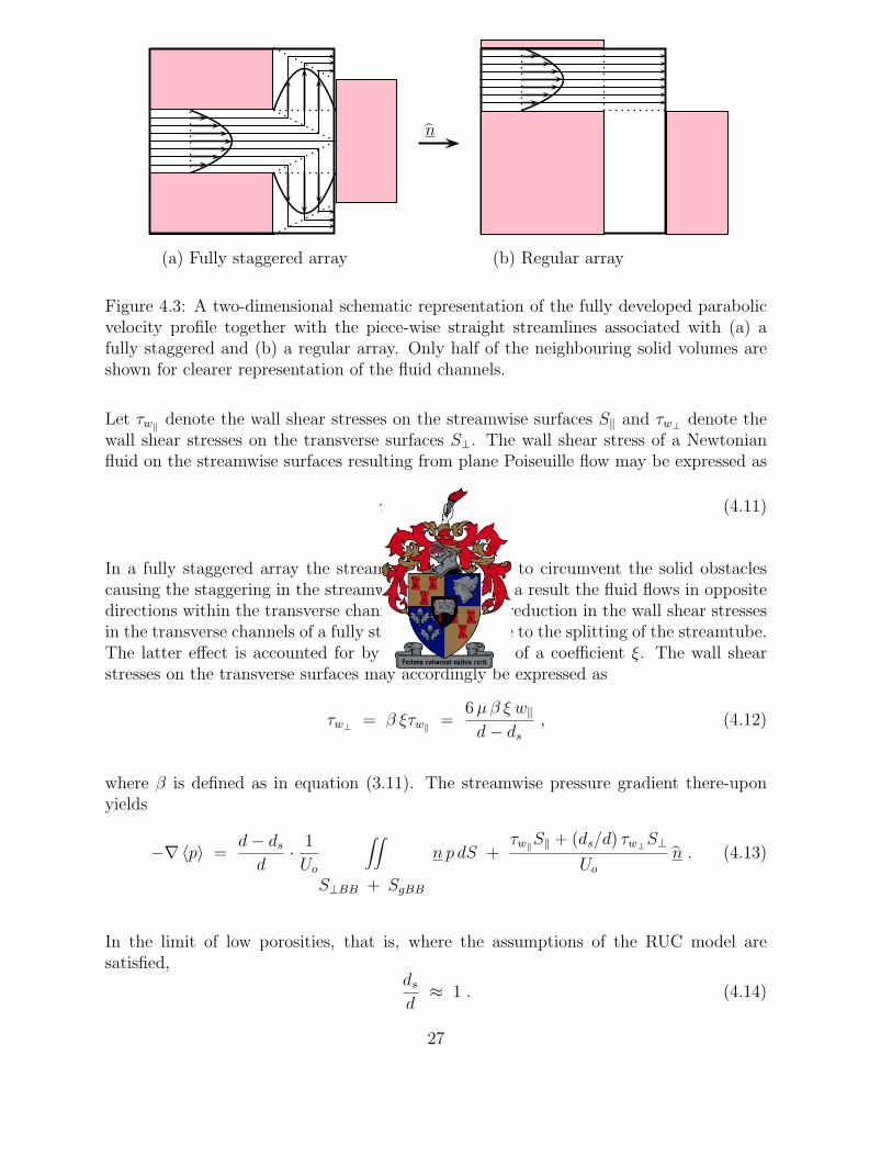
Figure 4.3: A two-dimensional schematic representation of the fully developed parabolicvelocity profile together with the piece-wise straight streamlines associated with (a) afully staggered and (b) a regular array. Only half of the neighbouring solid volumes areshown for clearer representation of the fluid channels.
Let τw‖denote the wall shear stresses on the streamwise surfaces S‖ and τw⊥
denote thewall shear stresses on the transverse surfaces S⊥. The wall shear stress of a Newtonianfluid on the streamwise surfaces resulting from plane Poiseuille flow may be expressed as
τw‖=
6µw‖
d− ds
. (4.11)
In a fully staggered array the streamwise flux divides to circumvent the solid obstaclescausing the staggering in the streamwise direction. As a result the fluid flows in oppositedirections within the transverse channels leading to a reduction in the wall shear stressesin the transverse channels of a fully staggered array due to the splitting of the streamtube.The latter effect is accounted for by the introduction of a coefficient ξ. The wall shearstresses on the transverse surfaces may accordingly be expressed as
τw⊥= β ξτw‖
=6µβ ξ w‖
d− ds
, (4.12)
where β is defined as in equation (3.11). The streamwise pressure gradient there-uponyields
−∇〈p〉 =d− ds
d· 1
Uo
∫∫
S⊥BB + SgBB
n p dS +τw‖
S‖ + (ds/d) τw⊥S⊥
Uo
n . (4.13)
In the limit of low porosities, that is, where the assumptions of the RUC model aresatisfied,
ds
d≈ 1 . (4.14)
27
It thus follows that
−∇〈p〉 =d− ds
d· 1
Uo
∫∫
S⊥BB + SgBB
n p dS +S‖ + β ξ S⊥
Uo
τw‖n . (4.15)
The remaining surface integral was shown by Lloyd (2003), to be expressible in terms ofthe gradient of the average pressure. The same procedure as for two-dimensional arraysof squares can be applied to three-dimensional arrays in the following way: Splitting thesurface integral of equation (4.15) into one applicable to a fully staggered array and theother applicable to a regular array, yields
d− ds
d· 1
Uo
∫∫
S⊥BB + SgBB
n p dS =d− ds
d· 1
Uo
∫∫
S⊥BB
n p dS +
d− ds
d· 1
Uo
∫∫
SgBB
n p dS . (4.16)
The surface integral applicable to a fully staggered array may be expressed as
d− ds
d· 1
Uo
∫∫
S⊥BB
n p dS =(d− ds)
d
[d2
s
Uo
(∆p+ δp)
]n
= −U⊥ + Ug
Uf
∇〈p〉
=
(U‖ + Ut
Uf
− 1
)∇〈p〉 , (4.17)
where ∆p is the total change in pressure in the streamwise volume and δp is the totalchange in pressure in the transverse volume. The above result (Lloyd (2003)) is obtainedfrom the fact that
∆p+ δp
dn = −Uo
Uf
∇〈p〉 . (4.18)
The surface integral applicable to a regular array may be expressed as
d− ds
d· 1
Uo
∫∫
SgBB
n p dS =(d− ds)
d
[d2
s
Uo
∆p
]n
= −U⊥ + Ug
Uf
∇〈p〉
=
(U‖ + Ut
Uf
− 1
)∇〈p〉 , (4.19)
28
resulting from the fact that∆p
dn = −Uo
Uf
∇〈p〉 . (4.20)
The streamwise pressure gradient applicable to both a fully staggered and a regular arraymay thus be expressed as
−∇〈p〉 =
(U‖ + Ut
Uf
− 1
)∇〈p〉 +
S‖ + β ξ S⊥
Uo
τw‖n , (4.21)
or after simplification
−∇〈p〉 =
(Uf
U‖ + Ut
)S‖ + β ξ S⊥
Uo
τw‖n . (4.22)
The streamwise pressure gradient may there-upon be expressed as
A well-known expression for relating the external pressure drop to the superficial velocityis Darcy’s empirical law for steady unidirectional creeping flow of a Newtonian fluidthrough an unbounded isotropic granular porous medium of uniformly sized particles, i.e.
∆p
L=
µ
kq , (4.25)
where ∆p is the pressure drop across the porous medium of length L and k is the Darcy orhydrodynamic permeability. For unidirectional flow in the positive x-direction of a Carte-sian coordinate system, the streamwise pressure drop for Newtonian flow may, analogouslyto Darcy’s equation, be expressed as
−dp
dx= µf00 q , (4.26)
29
where f00 is the shear factor of which the first subscript denotes the asymptotic limit oflow Reynolds number flow and the second subscript denotes the asymptotic limit of lowporosity. It thus follows that the shear factor f00 relates to the hydrodynamic permeability,which is dependent on the porous microstructure, as follows
f00 =1
k. (4.27)
The shear factor f00 may consequently be expressed as
f00 =12 (2 + β ξ)(1 − ǫ)4/3
d2s (1 − (1 − ǫ)1/3) (1 − (1 − ǫ)2/3)
2 . (4.28)
The dimensionless shear factor F00 = f00 d2s, describing the flow of a Newtonian fluid
through both a fully staggered- and a non-staggered regular array, is thus given by
F00 =12 (2 + β ξ)(1 − ǫ)4/3
(1 − (1 − ǫ)1/3) (1 − (1 − ǫ)2/3)2 , (4.29)
or in terms of the dimensionless hydrodynamic permeability K = k/d2s,
K =
(1 − (1 − ǫ)1/3
) (1 − (1 − ǫ)2/3
)2
12 (2 + β ξ)(1 − ǫ)4/3. (4.30)
The transverse pore sections of a fully staggered array, in which the fluid flows in oppositedirections, are assumed to be equal in volume. Therefore it is assumed that, similarly asin the case of two-dimensional flow, ξ = 1
2for a fully staggered array. For a regular array
ξ = 1, since in a regular array no splitting of the streamtube occurs. Due to the factthat a regular array does not contain any transverse channels, it follows that for a regulararray β = 0. The determination of the value of β for a fully staggered array requiresfurther analysis and will be addressed in the following subsection.
4.1.1 Evaluation of the coefficient β
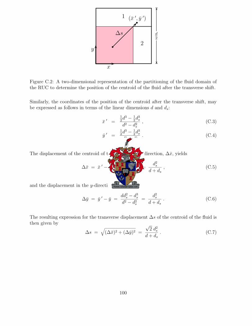
The RUC associated with a fully staggered array can be partitioned into four symmetricparts, as illustrated in Figure 4.4. Consider one of the four symmetric parts of the RUCpresented in Figure 4.4. The bottom left hand part is arbitrarily chosen for illustrationpurposes. Let ∆s denote the displacement of the centroid of the fluid due to the shiftingthereof to circumvent obstacles for streamwise discharge. Figure 4.5 illustrates the trans-verse displacement ∆s for fluid discharge through the RUC corresponding to the bottomleft hand part of Figure 4.4. Let ∆x and ∆y respectively denote the transverse displace-ment of the centroid of the fluid in the x- and y-directions of a Cartesian coordinatesystem, as shown in Figure 4.5.
30
Figure 4.4: A two-dimensional illustration of the partitioning of the RUC associated witha fully staggered array into four symmetric parts.
∆s
∆x
∆y
y
x
d2
ds
2
Figure 4.5: Illustration of the transverse displacement ∆s of the centroid of the fluid fordischarge through the RUC corresponding to the bottom left hand part of the RUC shownin Figure 4.4.
The fluid volume in the transverse channels U⊥ may be expressed as
U⊥ = Ap⊥∆s , (4.31)
where Ap⊥ denote the cross-sectional flow area available for fluid discharge through thetransverse channels within the RUC. Conservation of mass requires that
Q = w‖Ap‖ = w⊥Ap⊥ , (4.32)
where Q denotes the volumetric flow rate. From equations (4.31), (4.32) and (3.11) itfollows that β may be expressed as
β =Ap‖∆s
U⊥
. (4.33)
31
The displacement ∆s may be obtained by determining the position of the centroid of thefluid before and after the transverse shift (Appendix C), yielding
∆s =
√2 d2
s
d+ ds
. (4.34)
It thus follows that the value of β for a fully staggered array, yields
β =(d2 − d2
s)
d2sdf
√2 d2
s
d+ ds
=√
2 . (4.35)
Since each of the four symmetric parts of the RUC shown in Figure 4.4, yields the samevalue for β and contributes evenly to the nett effect of the flow field, β =
√2 may be
taken as the average value for β for a fully staggered array.
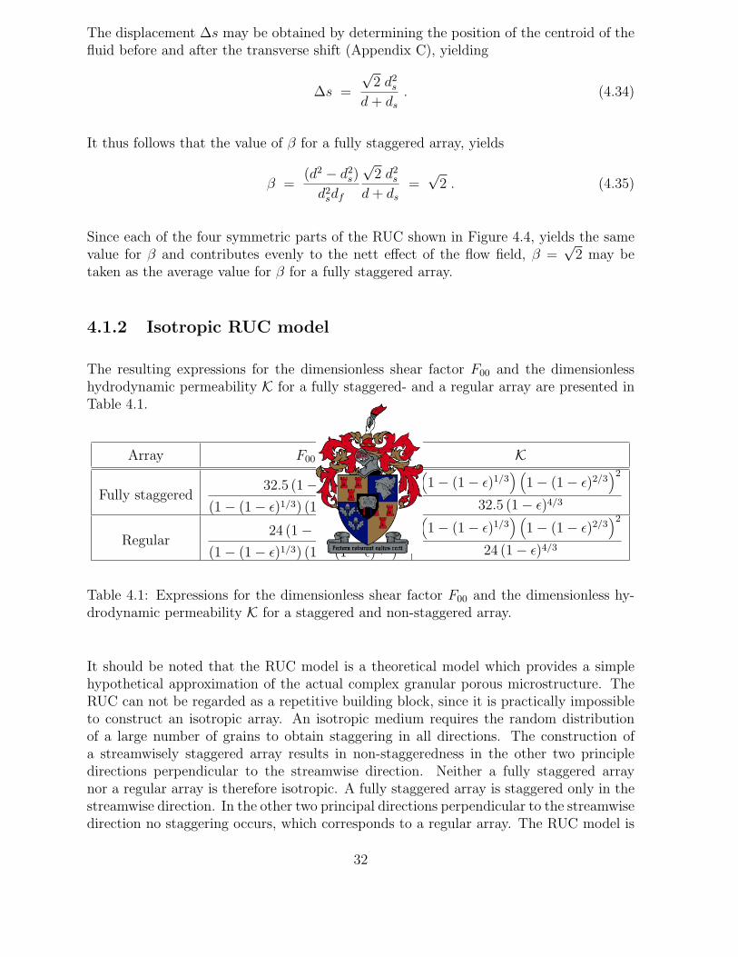
4.1.2 Isotropic RUC model
The resulting expressions for the dimensionless shear factor F00 and the dimensionlesshydrodynamic permeability K for a fully staggered- and a regular array are presented inTable 4.1.
Array F00 K
Fully staggered32.5 (1 − ǫ)4/3
(1 − (1 − ǫ)1/3) (1 − (1 − ǫ)2/3)2
(1 − (1 − ǫ)1/3
) (1 − (1 − ǫ)2/3
)2
32.5 (1 − ǫ)4/3
Regular24 (1 − ǫ)4/3
(1 − (1 − ǫ)1/3) (1 − (1 − ǫ)2/3)2
(1 − (1 − ǫ)1/3
) (1 − (1 − ǫ)2/3
)2
24 (1 − ǫ)4/3
Table 4.1: Expressions for the dimensionless shear factor F00 and the dimensionless hy-drodynamic permeability K for a staggered and non-staggered array.
It should be noted that the RUC model is a theoretical model which provides a simplehypothetical approximation of the actual complex granular porous microstructure. TheRUC can not be regarded as a repetitive building block, since it is practically impossibleto construct an isotropic array. An isotropic medium requires the random distributionof a large number of grains to obtain staggering in all directions. The construction ofa streamwisely staggered array results in non-staggeredness in the other two principledirections perpendicular to the streamwise direction. Neither a fully staggered arraynor a regular array is therefore isotropic. A fully staggered array is staggered only in thestreamwise direction. In the other two principal directions perpendicular to the streamwisedirection no staggering occurs, which corresponds to a regular array. The RUC model is
32
assumed to be isotropic with respect to the average geometric properties of the granularporous medium. Consequently, an isotropic RUC model is introduced by taking theaverage of one fully staggered array and two regular arrays, i.e.
F00 =1 ×
[12(2 + (1/
√2))]
+ 2 × [12 (2 + 0)]
3×
(1 − ǫ)4/3
(1 − (1 − ǫ)1/3
) (1 − (1 − ǫ)2/3
)2
. (4.36)
The existing RUC model also adopted the assumption of average geometrical isotropy,but the assumption was never mathematically justified as above. The final present RUCmodel for steady laminar flow of an incompressible Newtonian fluid through isotropichomogeneous granular porous media of low to moderate porosity in the limit of lowReynolds number flow, expressed as F00, f00 d
2 and K, are presented in Table 4.2.
Dimensionless parameter Isotropic RUC model
F0026.8 (1 − ǫ)4/3
(1 − (1 − ǫ)1/3
) (1 − (1 − ǫ)2/3
)2
f00 d2 26.8 (1 − ǫ)2/3
(1 − (1 − ǫ)1/3
) (1 − (1 − ǫ)2/3
)2
K(1 − (1 − ǫ)1/3
) (1 − (1 − ǫ)2/3
)2
26.8 (1 − ǫ)4/3
Table 4.2: Dimensionless expressions for the RUC model in the limit of low Reynoldsnumber flow.
4.2 Comparison with granular models from literature
4.2.1 Hydraulic diameter
The hydraulic diameter is a length scale most commonly used for direct comparisonbetween flow through systems of different geometrical structure. The hydraulic diameterDh for capillary tube flow of uniform cross-section is defined as
Dh = 4Rh , (4.37)
where Rh denotes the hydraulic radius, defined as
Rh =cross-sectional area available for flow
wetted perimeter. (4.38)
33
For flow through porous media Rh may also be expressed as (Bird et al. (2002))
Rh =void volume/volume of bed
wetted surface/volume of bed=
ǫ
a, (4.39)
where a is referred to as the specific surface and relates to the total solid surface pervolume of particles av, i.e. the solid specific surface, through
a = av(1 − ǫ) . (4.40)
The solid specific surface av is used to extend the definition of the hydraulic radius toaccount for beds of non-uniformly sized particles in order to obtain an average diameter.In effect, the assemblage of non-uniformly sized particles is replaced with an assemblageof uniformly sized particles, having the same ratio of total solid surface per volume ofparticles as the original assemblage, but not the same number of particles. Therefore theactual particle diameter does not enter into the determination of the hydraulic radius.The (average) hydraulic diameter may consequently be expressed in terms of the specificsurface as follows
Dh =6
av
. (4.41)
The reason for the latter definition for the hydraulic diameter is to obtain the desiredresult of
Dh =6
av
= 6(4/3)πR3
4πR2= 2R = Dp , (4.42)
for an assemblage of uniformly sized spherical particles of radius R and diameter Dp. InRUC notation it follows that for an assemblage of uniformly sized cubes of length ds,
Dh =6
av
= 6d3
s
6 d2s
= ds . (4.43)
From equations (4.39) to (4.41) it follows that the relationship between the hydraulicradius and the hydraulic diameter may be expressed in terms of the porosity as
Rh =ǫDh
6 (1 − ǫ). (4.44)
The present RUC model is to be compared with other granular models from the literature.Based on the results of equations (4.42) and (4.43), it will henceforth be assumed thatthe diameter of a sphere in an assemblage of uniformly sized spherical particles is equalto the length of the cube ds in the RUC model.
34
4.2.2 Dimensionless permeability and shear factor
The models to be compared with the present RUC model for predicting flow in the lowReynolds number flow regime are presented in Table 4.3. All these models considerthree-dimensional, steady, laminar flow of an incompressible Newtonian fluid through ahomogeneous isotropic granular porous medium.
Model Model type Packing material
Blake-Kozeny Capillary Spheres
Macdonald et al. (1979) Empirical verification Spheres
Dagan (1989) Statistical averaging Cubes
Happel (1958) Concentric cell Spheres
Existing RUC Spatial averaging Cubes
Table 4.3: Granular models for predicting flow in the low Reynolds number flow regime.
The Blake-Kozeny equation (Appendix D.1) concerns fully developed laminar flow of aNewtonian fluid through a packed bed of smooth uniformly sized spherical particles in dieDarcy regime. The flow through the interstices of the packed column of uniform diameteris regarded as flow through a bundle of uniform parallel capillary tubes. To account for thetortuous flow path actually followed by the traversing fluid, Carman (1937) introduceda tortuosity factor into the Blake-Kozeny equation. The dimensionless hydrodynamicpermeability K as predicted by the Blake-Kozeny equation, may be expressed as
K =ǫ3
150 (1 − ǫ)2, (4.45)
and is valid for ǫ < 0.5. Macdonald et al. (1979) suggested a coefficient value of 180 for theBlake-Kozeny equation, instead of the value of 150, which corresponds to the coefficientvalue proposed by Carman (1937) in the Carman-Kozeny-Blake equation (Appendix D.2).His proposal was based on a large number of experimental results. The dimensionlesshydrodynamic permeability K, as suggested by the empirical verification of Macdonaldet al. (1979), may thus be expressed as
K =ǫ3
180 (1 − ǫ)2. (4.46)
Dagan (1989) proposed a model based on a statistical volume averaging approach for pre-dicting the permeability through a granular porous medium of low porosity. The porousmedium is regarded as a network of three-dimensional planar fissures with interconnected
35
pores of uniform aperture. The random orientation of the fissures is described by a proba-bility distribution function. Fully developed laminar flow is assumed to prevail throughoutall pore sections. The hydrodynamic permeability as predicted by the model of Dagan(1989), in which a uniform superficial velocity field is assumed, is given by
k =ǫ b2
18, (4.47)
where b denotes the constant aperture between the fissures. For flow between parallelplates a distance b apart, it follows that
Dh = 2 b . (4.48)
From equations (4.37), (4.40) and (4.41), it follows that
b =ǫDh
3 (1 − ǫ). (4.49)
The dimensionless hydrodynamic permeability K as predicted by the model of Dagan(1989), may thus be expressed as
K =ǫ3
162 (1 − ǫ)2. (4.50)
Happel (1958) proposed a concentric spherical cell model for predicting the permeabil-ity through a random assemblage of spheres in the creeping flow regime over the entireporosity range. The spherical shape was chosen since many particles approximate thespherical form. The assemblage of spheres is regarded as a periodic array consisting ofidentical spherical unit cells of which each cell contains a single solid sphere surroundedby a fluid envelope. The solid sphere is positioned concentrically with the outer sphericalfluid envelope. The concentric spheres are assumed to be stationary with a traversingfluid entering the cell with a uniform approaching velocity q. The fluid is free to passover the outer surface of the cell. The outside surface of each cell is assumed to be fric-tionless, that is, the normal velocity and the tangential stresses on the outer sphere areassumed to be zero. No friction occurs between adjacent fluid envelopes. The porosityof the spherical cell is assumed to be equal to the porosity of the entire assemblage. Thepressure gradient prediction over the packed bed was determined by solving the Stokes’sequations subjected to the boundary conditions ensuring frictionless outer surfaces. Thedimensionless hydrodynamic permeability K as predicted by the model of Happel (1958),may be expressed as
K =
(3 − 9
2(1 − ǫ)1/3 + 9
2(1 − ǫ)5/3 − 3 (1 − ǫ)2
)
18 (1 − ǫ) (3 + 2(1 − ǫ)5/3). (4.51)
The dimensionless hydrodynamic permeability K as predicted by the existing RUC modelis given by
K =ǫ(1 − (1 − ǫ)1/3
) (1 − (1 − ǫ)2/3
)
41 (1 − ǫ)4/3. (4.52)
36
A graphical comparison for the permeability prediction of the models presented in Table4.3 with the present low porosity RUC model is shown in Figure 4.6.
Figure 4.6: Comparison between hydrodynamic permeability predictions.
Graphically it appears as if there is very little difference between the present and exist-ing RUC models. However, from an analytical point of view the difference between themodels is quite significant. The fundamental differences between the two models are thefollowing: The present RUC model mathematically justifies the assumption of average ge-ometrical isotropy, which was not accounted for in the existing model. The contributionof the transverse pressure term in the surface integral of equation (4.1) to the streamwisepressure gradient, caused by the transverse shear stresses, was neglected in the existingmodel. The square in the numerator of the expression for K of the present RUC modelin Table 4.2, which is absent in the expression for the existing model, is the result ofthis discrepancy. The existing RUC model considered only a staggered array in which nosplitting of the streamtube occurs and no stagnant regions are present, which is the reasonfor the difference in coefficient values produced by the two models. The close correspon-dence between all the models in Figure 4.6 show that the capillary models (Blake-Kozenyand Macdonald), the submerged object model (Happel) and the models based on volumeaveraging (RUC models and Dagan) are all adequate models for modelling laminar flowthrough granular porous medium of low to moderate porosities. It is very satisfactorythat the present RUC model agree so well with the other models which follow differentmodelling strategies. The validity of the analytical closure modelling procedure with thepore-scale RUC model is therefore justified in this manner. Since the models are all lowto moderate porosity models, except for the extended range of the spherical cell model,the discrepancies observed at ǫ > 0.8 are expected and may be attributed to the differ-ent physical flow process occurring at high porosities due to the absence of neighbouringgrains. At high porosities a flow by situation occurs instead of flow through.
37
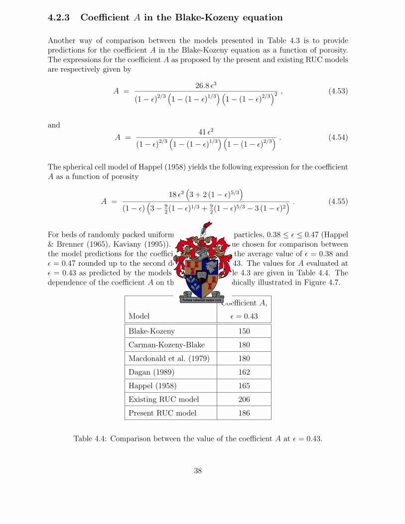
4.2.3 Coefficient A in the Blake-Kozeny equation
Another way of comparison between the models presented in Table 4.3 is to providepredictions for the coefficient A in the Blake-Kozeny equation as a function of porosity.The expressions for the coefficient A as proposed by the present and existing RUC modelsare respectively given by
A =26.8 ǫ3
(1 − ǫ)2/3(1 − (1 − ǫ)1/3
) (1 − (1 − ǫ)2/3
)2 , (4.53)
and
A =41 ǫ2
(1 − ǫ)2/3(1 − (1 − ǫ)1/3
) (1 − (1 − ǫ)2/3
) . (4.54)
The spherical cell model of Happel (1958) yields the following expression for the coefficientA as a function of porosity
A =18 ǫ3
(3 + 2 (1 − ǫ)5/3
)
(1 − ǫ)(3 − 9
2(1 − ǫ)1/3 + 9
2(1 − ǫ)5/3 − 3 (1 − ǫ)2
) . (4.55)
For beds of randomly packed uniformly sized spherical particles, 0.38 ≤ ǫ ≤ 0.47 (Happel& Brenner (1965), Kaviany (1995)). The porosity value chosen for comparison betweenthe model predictions for the coefficient A is taken as the average value of ǫ = 0.38 andǫ = 0.47 rounded up to the second decimal, i.e. ǫ = 0.43. The values for A evaluated atǫ = 0.43 as predicted by the models presented in Table 4.3 are given in Table 4.4. Thedependence of the coefficient A on the porosity is graphically illustrated in Figure 4.7.
Coefficient A,
Model ǫ = 0.43
Blake-Kozeny 150
Carman-Kozeny-Blake 180
Macdonald et al. (1979) 180
Dagan (1989) 162
Happel (1958) 165
Existing RUC model 206
Present RUC model 186
Table 4.4: Comparison between the value of the coefficient A at ǫ = 0.43.
38
0 0.2 0.4 0.6 0.8 1140
160
180
200
220
240
260
280
300
320
340
360
Porosity, ∈
Coe
ffici
ent
A
Eqn (4.53)Eqn (4.54)Eqn (4.55)Blake−Kozeny ( A = 150)Macdonald ( A = 180)Dagan ( A = 162)
∈ = 0.43
Figure 4.7: Dependence of the coefficient A on porosity.
For porosities ranging from ǫ = 0.34 to ǫ = 0.48, empirical values for A ranging fromA = 157 to A = 180 has been obtained, with an average value of A = 169 (Macdonaldet al. (1979)). For the same porosity range the values for A predicted by the presentRUC model range from 183.5 to 187 with an average value of 185. According to a surveyof Kemblowski & Michniewics (1979), the values suggested for the coefficient A for flowof Newtonian fluids through granular beds, range from A = 150 to A = 200, but themajority of references suggest the value of A = 180 and most commonly used are thevalues of A = 180, determined by Carman (1937), and A = 150, proposed by Ergun(1952). It is encouraging that the value of A = 186 for ǫ = 0.43, suggested by the presentRUC model, verges upon this range and the excellent correspondence with the value ofA = 180, suggested by Carman (1937) and Macdonald et al. (1979), is very satisfying andclearly shows the improvement on the existing RUC model (A = 206).
4.2.4 High porosity model
In the limit of low Reynolds number flow the RUC model increasingly loses its validityas the porosity ǫ approaches unity due to the failure of the applicability of the assump-tion of flow between parallel plates. Churchill & Usagi (1972) introduced an asymptotematching technique in which two expressions, each of which dominates in its own regionof applicability, may be matched to obtain a general expression over the entire range ofparameter values. By application of this technique it is possible to match the RUC modelwith a model for predicting flow conditions in the asymptotic limit of high porosities. Twohigh porosity models from the literature which are adequate for this purpose is the well-known drag model of Stokes (e.g. Chorlton (1967)) and the model of Hasimoto (1958).As opposed to the low porosity models which provide an expression for the pressure drop
39
prediction over an assemblage of submerged grains, the high porosity models provide anexpression for the drag force on a single grain within the assemblage, due to the absenceof neighbouring grains. At high porosities a different physical flow process occurs: thegrains are far enough apart so that the disturbances produced by an individual grain onthe flow behaviour is not affected by the disturbances produced by its neighbours. Stokes’flow concerns the steady motion of an unbounded incompressible Newtonian fluid witha uniform approaching velocity q past an isolated stationary sphere of radius R in thecreeping flow regime. The equation resulting from omission of the inertial terms from theNavier-Stokes equation, together with the continuity equation, are known as the Stokes’equations. The drag force F exerted by the sphere on the fluid is obtained by solving theStokes’ equations subjected to a no-slip boundary condition, yielding
F = 6π µR q . (4.56)
Equation (4.56) applies for ǫ ≈ 1. From equation (4.26) it follows that the relationbetween the shear factor f01 and the drag force F may be expressed as
−dp
dx= µf01 q =
Fd3
, (4.57)
where the first subscript of the shear factor f01 denotes the asymptotic limit of lowReynolds number flow and the second subscript denotes the asymptotic limit of highporosity. Assuming that the diameter of the sphere is equivalent to the length of the cubein the RUC model, i.e. 2R = ds, yields
f01 =3π (1 − ǫ)
d2s
, (4.58)
or in terms of the dimensionless shear factor F01 the Stokes’ drag may be described as
F01 = 3π (1 − ǫ) . (4.59)
The Stokes’ drag serves as a basis for the introduction of many other high porosity modelsfrom the literature. An example is the model of Hasimoto (1958) concerning the steadymotion of an incompressible Newtonian fluid past a periodic array of small particles in adilute medium. A periodic array of uniform spheres is constructed by repeating a basicunit cell with spheres placed at the corners of each cell. Hasimoto replaced each sphereby a point force, retarding the motion of the fluid, and modified the Stokes equationsto compensate for the discontinuous force field by means of the Dirac delta function andFourier series. A no-slip boundary condition is assumed at the surface of each sphere.The flow past three different types of cubic lattices is considered, namely simple, body-centered and face-centered cubic lattices. The drag force for flow past a single sphere ofradius R in a body-centered or face-centered cubic array is given by
F =6π µR q
1 − 1.791 (1 − ǫ)1/3+ O
(R3). (4.60)
40
For dilute suspensions, that is ǫ ≈ 1, the series expansion,
1
1 − 1.791(1 − ǫ)1/3≈ 1 + 1.791 (1 − ǫ)1/3 +O
((1 − ǫ)2/3
), (4.61)
can be used (Happel & Brenner (1965)) to approximate equation (4.41), yielding
F = 6π µR q(1 + 1.791 (1 − ǫ)1/3
)+ O
((1 − ǫ)2/3
). (4.62)
Neglecting the higher order terms, the drag force may be expressed in terms of the shearfactor f01 as follows
f01 =3π (1 − ǫ)
d2s
(1 + 1.791 (1 − ǫ)1/3
), (4.63)
or in terms of the dimensionless shear factor F01 the model of Hasimoto (1958) may bedescribed as
F01 = 3π (1 − ǫ)(1 + 1.791 (1 − ǫ)1/3
). (4.64)
Since external boundary effects are neglected in this work, the physical flow process inwhich the grains move at a uniform average velocity through a stationary fluid or thegrains remain stationary in the presence of a traversing fluid with a uniform averagevelocity, may be treated as mathematically equivalent (Happel (1958)).
4.2.5 Asymptote matching of low and high porosity models
Application of the asymptote matching technique of Churchill & Usagi (1972) yields thefollowing general expression for the shear factor in the limit of low Reynolds number flow,F0, applicable over the entire porosity range
F0 = ((F00)s + (F01)
s)1/s , (4.65)
where s denotes a shifting parameter. The numerical value of the shifting parameterdetermines how closely the matching curve follows the two asymptotic limits in the tran-sition regime. For simplicity the value s = 1 is chosen which yields a simple superpositionof the two asymptotic limits. Asymptote matching of the RUC model with Stokes’ dragmodel yields
F0 =26.8 (1 − ǫ)
4
3
(1 − (1 − ǫ)
1
3
) (1 − (1 − ǫ)
2
3
)2 + 3π (1 − ǫ) , (4.66)
and matching the RUC model with the model of Hasimoto (1958) one obtains
F0 =26.8 (1 − ǫ)
4
3
(1 − (1 − ǫ)
1
3
) (1 − (1 − ǫ)
2
3
)2 + 3π (1 − ǫ)(1 + 1.791 (1 − ǫ)1/3
). (4.67)
41
0 0.2 0.4 0.6 0.8 1
10−2
100
102
104
106
108
1010
Porosity, ∈
Dim
ensi
onle
ss s
hear
fact
or,
F0
Table 4.2Eqn (4.59)Eqn (4.64)Eqn (4.66)Eqn (4.67)
Figure 4.8: Asymptote matching of the RUC model with high porosity models.
The asymptote matching of the RUC model with the Stokes’ drag and the model ofHasimoto (1958) is shown in Figure 4.8 for all porosity values. Compared to the matchingcurves, the RUC model slightly under-predicts the frictional effects at ǫ ≈ 1. No physicalexplanation can be given regarding this matter, since the assumptions of the RUC modelare all invalid in this high porosity regime. Also note the small difference between the twomatching curves. Both the RUC/Stokes and RUC/Hasimoto models may therefore beregarded as adequate in predicting flow in the limit of low Reynolds number flow throughgranular porous media over the entire porosity range.
4.2.6 The Kozeny constant
The Kozeny constant kkoz (Appendix D.2), defined as
kkoz = k0
(Le
L
)2
, (4.68)
was introduced by Carman (1937) through modification of the Blake-Kozeny equationwith the velocity relationship,
u =q
ǫ
Le
L, (4.69)
where Le is the length of a tortuous channel, L is the length of a straight channel and k0 isan empirical shape factor which depends on the shape of the cross-section of the channel.Happel & Brenner (1965) defines the Kozeny constant as “a dimensionless number which,presumably, has the same numerical value for all random porous media, independently of
42
the size of the particles and the porosity” and presents the Kozeny constant alternativelyas
kkoz =ǫR2
h
k=
ǫ3
36K (1 − ǫ)2. (4.70)
The specific surface av is introduced into the definition for the hydraulic diameter (equa-tion (4.41)) to account for assemblages of non-uniformly sized particles. The purposeis to replace the assemblage of non-uniformly sized particles with an assemblage of uni-formly sized particles, having the same ratio of total solid surface per volume of particlesas the original assemblage, but not the same number of particles. This is the reasonfor the actual particle diameter not entering into the definition of the hydraulic radius.The hydraulic diameter in effect determines an average diameter for the assemblage ofnon-uniformly sized particles. Since it is assumed in this work that the spherical particlediameter is equivalent to the length ds of the solid cube in the RUC model, it follows thatequation (4.70) will indeed yield the same kkoz-value for an assemblage of spheres andcubes of the same porosity. The constancy of kkoz is supported by a considerable volumeof experimental data and can be predicted theoretically to a considerable degree of accu-racy (Happel & Brenner (1965)). Experimentally ko lies within the range 2.0 to 2.5 forflow through rectangular, elliptical and annular shapes. For pipe flow ko ranges between2.0 and 3.0 (Carman (1937)) and for flow between parallel plates ko = 3.0 (Kemblowski& Michniewics (1979)). Due to the very small variation in ko for flow through channels ofvarious cross-sections, the value of ko may be regarded as reasonably independent of shape(Happel & Brenner (1965)), leading to more or less constant kkoz-values as predicted byequation (4.68). Table 4.5 compares the kkoz-values predicted by the present RUC model(equation (4.70)) to the empirical values for kkoz presented by Carman (1937) for flowthough an assemblage of cubes and the cell model of Happel (1958) for flow through anassemblage of spheres.
Kozeny constant, kkoz
Present
Porosity, Carman RUC Happel
ǫ (cubes) (cubes) (spheres)
0.344 5.29 5.10 4.48
0.397 4.71 5.13 4.54
0.448 4.21 5.17 4.62
Table 4.5: Dependence of the Kozeny constant kkoz on low porosity values.
Sufficient experimental data on beds consisting of a variety of non-spherical particlesindicate that kkoz ≈ 5.0, independent of shape and porosity, from ǫ = 0.26 to ǫ = 0.8(Happel (1958)). For packed beds of uniformly sized spherical particles the Carman-Kozeny-Blake equation within the range ǫ = 0.26 to ǫ = 0.48, gives excellent correlation
43
with a Kozeny constant of k = 4.8 (Happel & Brenner (1965)). Table 4.5 shows theexcellent predictive capability of the present RUC model for obtaining kkoz ≈ 5.0 in theappropriate porosity range. Figure 4.9 compares the porosity dependence of the Kozenyconstant as predicted by the present RUC model with the predictive capability of thespherical cell model of Happel (1958).
0.4 0.5 0.6 0.7 0.8 0.9 10
10
20
30
40
50
60
70
80
Porosity, ∈
Koz
eny
cons
tant
, k ko
z
Eqn (4.70) & Table 4.2Eqns (4.70) & (4.51)
Figure 4.9: Porosity dependence of the Kozeny constant kkoz.
The correspondence between the kkoz-values predicted by the models for ǫ ranging between0.4 and 0.8 is very satisfactory. The reason for agreement of the values in this region isbecause the RUC model is a low to moderate porosity model whilst the spherical cellmodel is applicable over the entire porosity range. This also explains the reason for thediscrepancies observed between the two models at porosities above 0.8. Table 4.6 showsthe effect of matching the present RUC model with the high porosity models of Stokes’ andHasimoto (1958) on the values of the Kozeny constant. A graphical comparison betweenthe kkoz-values presented in Table 4.6 is shown in Figure 4.10. The values proposed by theRUC/Hasimoto model are in slightly better agreement with the values of the sphericalcell model as the values predicted by the RUC/Stokes model. This is due to the largerfrictional effects predicted by the model of Hasimoto (1958) at ǫ < 1 than the Stokes’drag, since the model of Hasimoto (1958) considers a cubic array of particles and theStokes’ drag only a single isolated particle. The latter effect, however, presents a minordifference. The good correspondence of both models with the spherical cell model rendersboth the RUC/Stokes and RUC/Hasimoto models adequate in predicting the values ofthe Kozeny constant for all porosities larger than 0.4.
44
Kozeny constant, kkoz
Present RUC / RUC /
Porosity, Happel RUC Stokes Hasimoto
ǫ (spheres) (cubes) (cubes / spheres)
0.99 71.63 21.81 47.22 57.02
0.90 11.34 7.64 9.55 11.13
0.80 7.22 6.20 6.87 7.57
0.70 5.79 5.66 5.96 6.32
0.60 5.11 5.39 5.53 5.71
0.50 4.74 5.23 5.29 5.39
0.40 4.54 5.14 5.16 5.21
Table 4.6: Porosity dependence of the Kozeny constant.
Figure 4.10: Porosity dependence of the Kozeny constant for different models presented.
45
Chapter 5
Laminar inertial flow regime
This chapter involves the analytical closure modelling of the fluid-solid interaction withinthe RUC for predicting the streamwise pressure gradient in the steady laminar limit ofthe inertial flow regime where turbulence is not yet present.
5.1 Closure modelling at moderate to high porosities
Du Plessis & Van der Westhuizen (1993) modelled the pressure integral in the Forchheimerregime for laminar crossflow through prismatic porous media by an internal form dragcondition, analogous to the external form drag condition for flow past a single obstaclein the inertial flow regime. The same modelling procedure was applied to flow throughgranular porous media (Du Plessis (1992)). It was assumed that the solid cube is subjectto a pressure deficit of 1
2ρv2
pcd, resulting from the interstitial flow recirculation within theseparation zone. The velocity vp denotes the magnitude of the average pore velocity asopposed to the uniform approaching velocity far away from the solid in the case of flowpast an isolated sphere. The reason for the introduction of the average pore velocitywas to incorporate the effect of neighbouring solids on the pressure gradient. A value of√
2 was proposed for the drag coefficient cd to account for the larger average transversechannel velocity due to the less pore space available for transverse flow than for flow inthe streamwise direction. A different analytical closure modelling procedure, analogousto the procedure presented in Du Plessis (1994), will be presented in this work.
The microscopic inertial effects will be modelled through consideration of interstitial flowrecirculation within the separation zone on the lee side of the solid cube with respectto the streamwise direction. In order to account for the influence, albeit assumed to beminimal, of the proximity of other cubes on the separation zone, the RUC model withinthe laminar limit of the inertial flow regime will be regarded as a moderate to high porositymodel (i.e. ǫ > 0.5). The flow within this limit, as within the low Reynolds number flowregime, will be assumed to be Newtonian. The streamwise pressure gradient resultingfrom volume averaging of the transport equations in which a uniform velocity field q is
46
assumed (Chapter 3), leads to
−∇〈p〉 =1
Uo
∫∫
Sfs
(n p− n · τ
)dS . (5.1)
In the steady laminar limit of the inertial flow regime the shear stresses yield viscousforces proportional to |q|1.5 (Du Plessis (1992)) when the inertial effects are modelledthrough consideration of flow development within the boundary layers. Modelling of themicroscopic inertial effects in the laminar limit through interstitial recirculation yields aproportionality of |∇p| ∝ |q|2. Since the latter proportionality lies well above the former,it will be assumed that the viscous forces may be neglected in the steady laminar limit ofthe inertial flow regime, yielding
−∇〈p〉 =1
Uo
∫∫
Sfs
n p dS . (5.2)
Although the streamlines change dramatically from the Darcy to the inertial flow regime,resulting from the development of boundary layers and local flow separation, the volumepartitioning of the fluid domain presented in chapter 3 will be used as an approximation forthe partitioning of the fluid domain within this limit in order to proceed with the closuremodelling procedure made available by the RUC model. The evaluation of the surfaceintegral of equation (5.2) over the respective surfaces, resulting from volume partitioningof the fluid domain, leads to
−∇〈p〉 =1
Uo
∫∫
S‖
n p dS +1
Uo
∫∫
S⊥
n p dS +1
Uo
∫∫
Sg
n p dS . (5.3)
At increasing porosities, the stagnant regions diminish and may therefore be discardedat very high porosities. Consequently, only high porosity fully staggered arrays will beconsidered within this limit. It thus follows that
−∇〈p〉 =1
Uo
∫∫
S‖
n p dS +1
Uo
∫∫
S⊥
n p dS . (5.4)
The parallel alignment of the streamwise surfaces of neighbouring cubes in the transversedirections, albeit assumed to be very far apart, results in the vectorial cancellation of thepressure on the streamwise surfaces, yielding
−∇〈p〉 =1
Uo
∫∫
S⊥
n p dS . (5.5)
47
The importance of the need to consider all possible locations of the RUC in the streamwisedirection was already mentioned in the closure modelling procedure for flow in the lowReynolds number flow regime and needs to be addressed once again. The two possiblechoices of RUC’s, considering all possible locations of an RUC associated with a fullystaggered array in the streamwise direction, are shown in Figure 5.1. The upstream anddownstream facing surfaces of the RUC with corner points AAAA cut through solid partsand the corresponding faces of the RUC with corner points BBBB do not cut throughany solid parts. S⊥AA and S⊥BB respectively denote the fluid-solid interfaces in U⊥ of theRUC with corner points AAAA and BBBB.
n
U⊥
U⊥
U⊥
U⊥
A AB B
A B A B
Figure 5.1: Schematic illustration of the two typical choices of RUC’s in a fully staggeredarray to consider all possible locations in the streamwise direction.
Repeating the weighting procedure for the relative frequency of occurrence of the twopossible RUC’s, shown in Figure 5.1, over a streamwise displacement d, leads to
−∇〈p〉 =ds
d· 1
Uo
∫∫
S⊥AA
n p dS +d− ds
d· 1
Uo
∫∫
S⊥BB
n p dS . (5.6)
Assuming that the pressure p on all facing pairs of transverse surfaces are equal, resultsin a vectorial cancellation of the pressures on these surfaces, that is
−∇〈p〉 =d− ds
d· 1
Uo
∫∫
S⊥BB
n p dS . (5.7)
At very high porosities, it follows that
d− ds
d≈ 1 , (5.8)
48
yielding
−∇〈p〉 =1
Uo
∫∫
S⊥BB
n p dS . (5.9)
The resulting surface integral represents the streamwise pressure drop over a solid cubecontained within an RUC associated with a high porosity fully staggered array. For furtheranalysis of the surface integral of equation (5.9), consider Figure 5.2, representing onlythe top half of the fully staggered array presented in Figure 5.1 for clearer illustrationpurposes. The interstitial recirculation within the separation zone on the lee side of thesolid cube with respect to the streamwise direction is clearly illustrated. Let S⊥U
denotethe upstream square surface of the cube and S⊥D
the downstream facing surface. Thevectors nU and nD denote the corresponding inwardly directed unit vectors normal to S⊥U
and S⊥D, respectively. Point A represents the stagnation point on the upstream facing
surface of the cube and point B on S⊥Drepresents the separation point of the dividing
streamline. Point C denotes the inflection point on the dividing streamline adjacent tothe separation zone of interstitial recirculation.
b
b
b
S‖
S‖
S⊥
S⊥DS⊥U
A
B
C
nU nD
n
n
n
n
Figure 5.2: A two-dimensional schematic representation of the interstitial recirculationpresent within the separation zone on the lee side of the solid cube with respect to thestreamwise direction. The bold dashed lines indicate the RUC boundaries.
Splitting the transverse surface integral accordingly into the upstream and downstreamtransverse facing surfaces yields
−∇〈p〉 =1
Uo
∫∫
S⊥D
nD pD dS +1
Uo
∫∫
S⊥U
nU pU dS , (5.10)
49
where pD denotes the pressure on S⊥Dand pU the pressure on S⊥U
. Due to the relativelylow velocities within the separation zone, the pressure on the downstream surface S⊥D
isassumed to be constant. It thus follows that
−∇〈p〉 =d2
s
Uo
pD nD +nU
Uo
∫∫
S⊥U
pU dS . (5.11)
The pressure pU will be approximated by applying Bernoulli’s equation along the dividingstreamline from the stagnation points A and B to the inflection point C. Bernoulli’sequation was, however, derived for non-viscous vortex free flow and the present modellingprocedure opposingly regards the flow of a viscous fluid. The applicability of Bernoulli’sequation is motivated by the fact that the dividing streamline along which the equationis applied, is adjacent to the region of recirculation and the viscosity of the fluid in thevicinity of the inflection point C is assumed to be negligible. Although the applicabilityof Bernoulli’s equation is a somewhat rough estimate for approximating the pressure onS⊥U
, fluids such as water and air which are most frequently used for modelling purposes,are low viscosity fluids which renders the approximation to be less harsh. Therefore,applying Bernoulli’s equation along the dividing streamline from the stagnation point Ato the inflection point C and assuming that the difference in elevation between the twopoints is negligible, leads to
pA
ρ+
v2A
2=
pC
ρ+
v2C
2, (5.12)
where vA and vC respectively denotes the magnitude of the interstitial fluid velocities atthe stagnation point A and the inflection point C. Since vA = 0 and since it may beassumed that the pressure at the separation point B also prevails within the separationzone (Roberson & Crowe (1985)), i.e. pC = pD, it follows that
pU = pA = pD +1
2ρ v2
C , (5.13)
yielding the following expression for the streamwise pressure gradient
−∇〈p〉 =d2
s
Uo
pD nD +nU
Uo
∫∫
S⊥U
pD dS +nU
Uo
∫∫
S⊥U
1
2ρ v2
C dS . (5.14)
Since, nU = −nD = n, the first two terms of equation (5.14) cancel, yielding
−∇〈p〉 =n
Uo
∫∫
S⊥U
1
2ρ v2
C dS . (5.15)
50
At relatively high velocities the interstitial flow field approximates a uniform velocityprofile, so that it seems reasonable to assume that the actual velocity at the inflectionpoint C may be approximated by the average transverse pore velocity, i.e.
vC ≈ w⊥ = β w‖ , (5.16)
The value of β for a fully staggered array is again taken as β =√
2 (chapter 4), since athigh velocities, the partial occupation of the region of flow recirculation in the transversechannel has negligible effect on the ratio of the average pore velocities w⊥ and w‖. Thestreamwise pressure gradient may there-upon be expressed as
−∇〈p〉 =ρw2
‖S⊥U
Uo
n
=ρw‖w‖ d
2s
d3(U0 = d3 , S⊥U
= d2s)
=ρ q q d d2
s
(d2 − d2s)
2(Eqn. (3.10))
=ρ q q (1 − ǫ)
ds (1 − (1 − ǫ)2/3)2 (Eqn. (3.4))
=µ q (1 − ǫ)
d2s (1 − (1 − ǫ)2/3)
2Rep (Eqn. (3.20)) (5.17)
For unidirectional flow of a Newtonian fluid in the positive x-direction of a Cartesiancoordinate system through a porous medium of local uniform porosity the streamwisepressure drop may, analogously to Forchheimer’s extension of Darcy’s law (Forchheimer(1901)) in which the higher order velocity term dominates, be expressed as
−dp
dx= µ f1 q . (5.18)
Here f1 denotes the shear factor in laminar limit of the inertial flow regime which maymay consequently be expressed as
f1 =(1 − ǫ)
d2s ǫ (1 − (1 − ǫ)2/3)
2Rep . (5.19)
The dimensionless shear factor F1 = f1 d2s, describing the flow of a Newtonian fluid through
granular media of high porosity, is thus given by
F1 =(1 − ǫ)
ǫ (1 − (1 − ǫ)2/3)2Rep . (5.20)
Equation (5.20) is equivalent to the expression proposed by the existing RUC model forflow in the steady laminar limit of the inertial flow regime. The validity of applying thetechnique of volume partitioning of the fluid domain in the laminar limit is therefore jus-tified since the volume partitioning technique was not applied in the modelling procedureof the existing RUC model within this regime.
51
5.2 Comparison with granular models from literature
5.2.1 Shear factor
There are very few models in the literature regarding flow through porous media in theForchheimer regime due to the complex nature of the flow characteristics, especially whereturbulence is involved. A well-known semi-empirical model for predicting the pressuregradient for the flow of a Newtonian fluid through packed beds of smooth uniformly sizedspherical particles in the Forchheimer regime, where highly turbulent flow was assumedto be present, is the empirical Burke-Plummer equation (Appendix D.3). The Burke-Plummer equation is based on the capillary-tube representation of turbulent flow througha packed bed and may be expressed in terms of the dimensionless shear factor F1 as follows
F1 =1.75 (1 − ǫ)
ǫ3Rep , (5.21)
and is valid for ǫ < 0.5. Macdonald et al. (1979) suggested a coefficient value of 1.80for the Burke-Plummer equation, instead of the value of 1.75. His proposal was basedon extensive experimental data. The dimensionless shear factor F1 as suggested by theempirical verification of Macdonald et al. (1979), may consequently be expressed as
F1 =1.8 (1 − ǫ)
ǫ3Rep . (5.22)
A graphical comparison between the present RUC model, the Burke-Plummer equationand the empirical verification of Macdonald et al. (1979) is shown in Figure 5.3 for ǫ = 0.43and Reynolds numbers within the Forchheimer regime. Although the RUC model forpredicting flow in the laminar inertial flow regime is a high porosity model, it seems thatthe assumptions made within the analytical modelling procedure apply equally well toporosities within the packed bed region. The excellent correspondence of the RUC modelwith the Burke-Plummer equation and with the empirical verification of Macdonald et al.(1979) over the entire Reynolds number range indicated in Figure 5.3, i.e. 10 < Rep <1000, demonstrates the ability of the RUC model to predict flow behaviour in the laminarinertial flow regime.
5.2.2 Coefficient B in the Burke-Plummer equation
The present RUC model may alternatively be compared to the Burke-Plummer equationby providing an expression for predicting the coefficient B in the Burke-Plummer equation(Appendix D.3) as a function of porosity i.e.
B =ǫ2
(1 − (1 − ǫ)2/3
)2 . (5.23)
52
101
102
103
102
103
104
105
Reynolds number, Rep
Dim
ensi
onle
ss s
hear
fact
or,
F1
Eqn (5.20)Eqn (5.21)Eqn (5.22)
Figure 5.3: Comparison of the dimensionless resistance factor F1 for ǫ = 0.43.
A comparison between the coefficient values predicted by the analytical and semi-empiricalmodels is given in Table 5.1 for ǫ = 0.43. The latter porosity value is chosen as the averagevalue corresponding to a granular packed bed.
Coefficient B,
Model ǫ = 0.43
Burke-Plummer 1.75
Macdonald 1.80
Present RUC 1.89
Table 5.1: Comparison of the coefficient B for ǫ = 0.43.
The porosity dependence of equation (5.23), together with the constant values proposedby the semi-empirical models, are graphically shown in Figure 5.4. For porosities rangingfrom 0.34 to 0.48 values for B ranging from 1.49 to 1.77 with an average value of 1.63 havebeen obtained experimentally (Macdonald et al. (1979)). For the same range of porositiesthe RUC model predicts values for B ranging from 1.85 to 1.97 with an average valueof 1.91. The objective of the RUC model with its simplifying assumptions was by nomeans to predict exact values, but rather to obtain values of the same order of magnitudeas the experimental values. In this respect the range of values predicted by the RUCmodel is very pleasing, especially the very good correspondence with the value proposedby Macdonald et al. (1979) at ǫ = 0.43.
53
0 0.2 0.4 0.6 0.8 11
1.5
2
2.5
Porosity, ∈
Coe
ffici
ent
B
Eqn (5.23)Burke−Plummer ( B =1.75)Macdonald ( B =1.80)
∈ = 0.43
Figure 5.4: Comparison of the dependence of the coefficient B on the porosity.
54
Chapter 6
Asymptote matching of laminarlimits
The RUC model proposed for the dimensionless shear factor in the asymptotic limit oflow Reynolds number flow and in the laminar limit of the inertial flow regime may bematched according to the asymptote matching technique introduced by Churchill & Usagi(1972) through application of the formula
F = (F s0 + F s
1 )1/s , (6.1)
to obtain an overall shear factor F applicable over the entire steady laminar flow regime.In order to obtain an analytical model for direct comparison with the semi-empirical Ergunequation (Appendix D.4), which is simply a superposition of two asymptotic limits, theshifting parameter s is chosen to be unity. A more accurate predictive expression may beobtained for values of the s greater than unity. Substituting for the corresponding shearfactors as predicted by the present RUC model into equation (6.1), yields
F =26.8 (1 − ǫ)4/3
(1 − (1 − ǫ)1/3
) (1 − (1 − ǫ)2/3
)2 +(1 − ǫ)
ǫ(1 − (1 − ǫ)2/3
)2Rep , (6.2)
For unidirectional flow of a Newtonian fluid in the positive x-direction of a Cartesiancoordinate system through a porous medium of local uniform porosity the streamwisepressure drop may, analogously to Forchheimer’s extension of Darcy’s law, be expressedas
−dp
dx= µF q , (6.3)
where, for s = 1, the overall shear factor is given by
F = F0 + F1 . (6.4)
55
The pressure drop prediction proposed by the present RUC model thus leads to
−dp
dx=
26.8 (1 − ǫ)4/3
d2s
(1 − (1 − ǫ)1/3
) (1 − (1 − ǫ)2/3
)2 µ q +(1 − ǫ)
ǫ ds
(1 − (1 − ǫ)2/3
)2 ρ q2 . (6.5)
If the RUC/Hasimoto model is introduced for the lower limit in equation (6.1) then theoverall shear factor becomes
F =26.8 (1 − ǫ)
4
3
(1 − (1 − ǫ)
1
3
) (1 − (1 − ǫ)
2
3
)2 + 3π (1 − ǫ)(1 + 1.791 (1 − ǫ)1/3
)
+(1 − ǫ)
ǫ(1 − (1 − ǫ)
2
3
)2Rep , (6.6)
with the corresponding pressure drop prediction given by
−dp
dx=
26.8 (1 − ǫ)4
3
(1 − (1 − ǫ)
1
3
) (1 − (1 − ǫ)
2
3
)2 µ q + 3π (1 − ǫ)(1 + 1.791 (1 − ǫ)1/3
)µ q
+(1 − ǫ)
ǫ ds
(1 − (1 − ǫ)2/3
)2 ρ q2 . (6.7)
Equations (6.5) and (6.7) are unified expressions for predicting the pressure drop forthe flow of an incompressible Newtonian fluid through a homogeneous isotropic granularporous medium within the entire steady laminar flow regime.
6.1 Comparison with the Ergun equation
The semi-empirical Ergun equation provides an expression for the pressure drop predictionfor the flow of an incompressible Newtonian fluid through a packed bed with uniformlysized spherical particles for Reynolds numbers ranging from the laminar to the highlyturbulent flow regime, i.e.
∆p
L= 150
(1 − ǫ)2
ǫ3µ q
D2h
+ 1.75(1 − ǫ)
ǫ3ρ q2
Dh
, (6.8)
where ∆p denotes the pressure drop over a bed of length L. The Ergun equation usuallyprovides good agreement with experimental data for ǫ < 0.5. Expressed in terms of theoverall shear factor the Ergun equation yields
F =150 (1 − ǫ)2
ǫ3+
1.75 (1 − ǫ)
ǫ3Rep , (6.9)
56
and the empirical verification of Macdonald et al. (1979) produces
F =180 (1 − ǫ)2
ǫ3+
1.8 (1 − ǫ)
ǫ3Rep . (6.10)
In Figure (6.1) results of the present RUC model is compared with the Ergun equationand the empirical verification of Macdonald et al. (1979) over the entire Reynolds numberrange.
10−1
100
101
102
103
104
102
103
104
105
106
Reynolds number, Rep
Ove
rall
shea
r fa
ctor
, F
Eqn (6.2)Eqn (6.6)Eqn (6.9)Eqn (6.10)
Darcyregime
Transitionregime
Forchheimerregime
Turbulence
Figure 6.1: Comparison of the present RUC model with the Ergun equation.
The excellent correspondence of the present RUC model with the empirical verificationof Macdonald et al. (1979) is rather astonishing, since the analytical model and the semi-empirical Ergun equation follow completely different modelling approaches. The agree-ment of the RUC model with the semi-empirical models at Rep > 1000 renders doubton the early onset of turbulence in porous media. The asymptote matching techniqueprovides a gradual transition from the Darcy to the inertial flow regime and proves tobe a very skilful technique for the matching of two asymptotic limits to obtain a unifiedexpression for predicting flow conditions over the entire matching domain. The presentRUC model may thus be regarded as a theoretical derivation of the semi-empirical Ergunequation. Despite the frequent use and modification of the Ergun equation in the liter-ature, it has received a great amount of criticism due to its lack of inter-connectedness(Dullien (1979)) and its limited applicability (Kaviany (1995)). The major advantage ofthe RUC model over the Ergun equation is that it contains no empirical factors. The co-efficients introduced into the model are all based purely on sound physical principles. Thepore-space of the RUC model is interconnected and provides a more realistic approxima-tion for flow through granular beds. Since a difference between the RUC model and theRUC/Hasimoto model is hardly discernable from Figure (6.1), it may be concluded thatthe RUC model, without the asymptote matching with the high porosity model of Hasi-moto in the low Reynolds number flow regime, is adequate for modelling flow conditions
57
over the entire Reynolds number flow regime. When flow behaviour in the low Reynoldsnumber flow regime alone is considered, the RUC/Hasimoto is the most promising model.
6.2 Critical Reynolds number
The Reynolds number associated with the location of the centre of the transition regionbetween the Darcy and Forchheimer regime, is called the critical Reynolds number, de-noted by Rec. The critical Reynolds number may be determined from equation (6.2) andthe resulting expression as a function of porosity is given by
Rec =26.8 ǫ (1 − ǫ)1/3
(1 − (1 − ǫ)1/3). (6.11)
Equation (6.11) defines a critical Reynolds number range of 0.1 ≤ Rec ≤ 75 for a porosityrange of 0.1 ≤ ǫ ≤ 1. This range of critical Reynolds numbers correspond exactly with theReynolds number range proposed by Dullien (1979) above which Darcy’s law is no longervalid for various porous media. Happel & Brenner (1965) state that the critical Reynoldsnumber at which separation first occurs in flow around a sphere is Rec = 17. For porositiesin the range 0.9 ≤ ǫ ≤ 0.95 equation (6.11) yields a range of critical Reynolds numbers of15 ≤ Rec ≤ 21. The value of Rec = 17 falls exactly within this range, underscoring thestatement by Happel & Brenner (1965).
58
Chapter 7
Non-Newtonian flow
A very large category of fluids used for industrial applications does not obey Newton’slaw of viscosity, which implies that the shear stress is no longer linearly proportionalto the shear rate. These structurally complex fluids of molecular weights larger than5000 are referred to as non-Newtonian fluids (Bird et al. (2002)). The viscosity of thesefluids depends strongly on the velocity gradient and is therefore a function of the char-acteristics of the porous medium and the rheological properties of the fluid. In contrastto incompressible Newtonian fluids, which solely require a measurement of the viscosity,non-Newtonian fluids require measurements of the viscosity together with possible secondorder effects such as normal stresses and viscoelastic responses. Non-Newtonian fluidsfind application in, for instance, the processing, pharmaceutical and petroleum industriesand in biological fields. Specific applications of the flow of non-Newtonian liquids throughporous media include the filtration of polymer solutions and the flow of aqueous polymersolutions through sand in secondary oil recovery operations (Christopher & Middleman(1965)). The velocity gradient dependent viscosity function takes on a variety of forms andtherefore non-Newtonian fluids may be divided into three broad categories (Harris (1977),Skelland (1967)): (1) purely viscous or time-independent fluids , (2) time-dependent flu-ids and (3) viscoelastic fluids. The purely viscous non-Newtonian fluids may in turnbe subdivided into the following groups: (i) shear-thinning or pseudoplastic fluids, (ii)shear-thickening or dilatant fluids and (iii) viscoplastic fluids. The shear-thinning fluidsare characterized by a decrease in apparent viscosity with increasing shear rate, whilstthe shear-thickening fluids exhibit an increase in apparent viscosity with increasing shearrate. The viscoplastic fluids are characterized by an additional finite yield stress whichis required to initiate the flow. The time-dependent fluids are those for which the shearrate is a function of both the magnitude and the duration of the shear stress at isother-mal conditions. Liquids for which the apparent viscosity increases with the duration ofthe shear stress are referred to as rheopectic fluids and those for which the apparentviscosity decreases with the duration of the shear stress are referred to as thixotropicfluids. Viscoelastic fluids possess both viscous and elastic properties. These fluids exhibitpartial recovery of deformation upon removal of stress and are associated with normalstress effects. In reality the classification of non-Newtonian fluids given above is by nomeans distinct or sharply defined since these fluids actually exhibit combinations of the
59
respective rheological flow characteristics; the classification simply serves as an aid formathematical modelling purposes. Various models are available in the literature for de-scribing the non-Newtonian flow behaviour within the distinctive categories. Only purelyviscous shear-thinning fluids will be considered in this work, due to the following reasons:The RUC model only concerns inelastic time-independent fluids. Time-dependent fluidsare seldom utilized in engineering design procedures and if required, purely viscous fluidscould be applied to time-dependent materials under isothermal steady flow conditions.Furthermore, the elastic properties of viscoelastic fluids are insignificant for fluid flowthrough channels of fixed cross section in the laminar flow regime (Skelland (1967)). Ex-amples of purely viscous shear-thinning fluids are polymer and rubber solutions, greases,soap, paints, gelatine, clay, milk, blood and liquid cement. A generalized expression formodel-ling the shear stress of both Newtonian and non-Newtonian fluids (Appendix E) isgiven by:
τyx = η (γ) |γ| , (7.1)
where τyx is the magnitude of the shear stress tensor τ for unidirectional fluid dischargein the positive x-direction. The simplest and most commonly used model to describethe rheological flow behaviour of purely viscous shear-thinning fluids for intermediateshear rates is the empirical Ostwald-de-Waele power law model (Skelland (1967)). Thedependence of the apparent viscosity η on the shear rate γ may be obtained from empiricalviscometry data and expressed as
η (γ) = K |γ|n−1 for n < 1 . (7.2)
Here K and n are constants characterizing the fluid and respectively referred to as theconsistency and behaviour indices. Since n is less than unity for shear-thinning fluids it isevident that the apparent viscosity decreases with increasing shear rate, which is definedas
γ =dv
dy, (7.3)
with v the actual speed of the fluid. The power law model may thus be expressed as
τyx = K |γ|n . (7.4)
The behaviour index n is the slope of the logarithmic plot of shear stress τyx versusshear rate γ which ranges from unity, resembling Newtonian flow behaviour, to zero. Theconsistency index K is calculated from the intercept on the τyx axis at unit shear rate(Skelland (1967)). The effect of normal stresses cannot be predicted or interpreted by thepower law model (Savins (1970)). For n = 1 the shear stress expression for describingNewtonian fluids is obtained (Appendix E).
60
7.1 RUC model for purely viscous power law flow
The RUC model was generalized for the first time by Du Plessis (1996) to predict theflow of purely viscous power law fluids through a variety of porous microstructures, in-cluding isotropic granular porous media. This section is based on the work of Smit & DuPlessis (1997) and (2000) which concerns the evaluation of the RUC model of Du Plessis& Masliyah (1991) for power law flow through isotropic granular porous media with pub-lished experimental data. The results of this chapter have been published (Woudberg et al.(2006)). The expression obtained for the streamwise pressure gradient for Newtonian flowin the low Reynolds number flow regime (equation (4.22)) is given by
−∇〈p〉 =
(Uf
U‖ + Ut
)S‖ + β ξS⊥
Uo
τw‖n . (7.5)
The latter expression may be generalized to account for non-Newtonian purely viscousflow by introducing the dependency of the apparent viscosity into the expression for thewall shear stress. The wall shear stress for power law flow between parallel plates adistance 2B apart, in which a no-slip boundary condition and fully developed flow areassumed (Appendix E.1) may be expressed as
τw‖= K
(2n+ 1
n
)n ( 2w‖
d− ds
)n
, n < 1 . (7.6)
Substituting for τw‖into equation (7.5) yields
−∇〈p〉 =
(Uf
U‖ + Ut
)S‖ + β ξS⊥
Uo
K(
2n+ 1
n
)n ( 2w‖
d− ds
)n
n . (7.7)
The following generalization of the pressure gradient for flow though a porous medium oflocal uniform porosity was introduced by Du Plessis (1996),
−ǫ∇〈p〉f = KFnqn−1q , (7.8)
so that for unidirectional discharge in the positive x-direction of a Cartesian coordinatesystem the streamwise pressure drop may be expressed as
−ǫdpdx
= KFn qn . (7.9)
Here Fn is the shear factor used in Du Plessis (1996) and relates to the shear factor usedin the present RUC model fn by
fn =Fn
ǫ. (7.10)
61
The streamwise pressure drop may there-upon be expressed as
−dp
dx= Kfnq
n (7.11)
wherefn = fn0
+ fn1, (7.12)
resulting from application of the asymptote matching technique of Churchill & Usagi(1972) with s = 1. The shear factor for power law flow in the limit of low Reynoldsnumbers, fn0
, as proposed by the present generalized RUC model is thus given by
fn0=
1
kn
=2n(4.47)(1 − ǫ)(n+3/3)
dn+1s
(1 − (1 − ǫ)1/3
)n (1 − (1 − ǫ)2/3
)n+1
(2n+ 1
n
)n
, (7.13)
where kn denotes the generalized hydrodynamic permeability. The expression obtainedfor the streamwise pressure gradient in the laminar limit of the inertial flow regime isgiven by
−∇〈p〉 =ρw2
‖S⊥U
Uo
n . (7.14)
Since the viscous forces are negligible in the steady laminar limit, the same expressionholds for the shear factor as for Newtonian flow (equation (5.19)) and by application ofequation (7.11) the following expression is obtained for the shear factor for power law flowin the laminar limit of the inertial flow regime,
fn1=
ρ q2−n(1 − ǫ)
ds ǫK(1 − (1 − ǫ)
2
3
)2 . (7.15)
It thus follows that the overall shear factor for purely viscous power law flow applicableover the entire steady laminar flow regime, fn, may be expressed as
fn =2n(4.47)(1 − ǫ)(n+3/3)
dn+1s
(1 − (1 − ǫ)1/3
)n (1 − (1 − ǫ)2/3
)n+1
(2n+ 1
n
)n[1 +
(1 − (1 − ǫ)2/3)
12 (4.47) ǫRepn
],
(7.16)
where the generalized particle Reynolds number Repn, defined in terms of the cube length
ds, is given by
Repn=
12 ρ dns q
2−n
K(1 − ǫ)n/3
(1 − (1 − ǫ)1/3)n
(1 − (1 − ǫ)2/3)2−n
(n
2 (2n+ 1)
)n
. (7.17)
The reason for expressing the Reynolds number Repn, as in equation (7.17), is simply
to be able to express the friction factor fn in the particular way that it is presented in
62
equation (7.16). Expressing fn in terms of the linear dimension d of the RUC, yields
fn =2n(4.47)(1 − ǫ)2/3
dn+1(1 − (1 − ǫ)1/3)n(1 − (1 − ǫ)2/3)n+1
(2n+ 1
n
)n[1 +
(1 − (1 − ǫ)2/3)
12 (4.47) ǫRepn
],
(7.18)
with the corresponding cell Reynolds number given by
Repn=
12 ρ dn q2−n
K
(1 − (1 − ǫ)1/3
)n
(1 − (1 − ǫ)2/3)2−n
(n
2 (2n+ 1)
)n
. (7.19)
The expression for the overall shear factor fn proposed by Smit & Du Plessis (1997) isgiven by
fn =2n 6 (1 − ǫ)2/3
dn+1(1 − (1 − ǫ)1/3)n(1 − (1 − ǫ)2/3)n
(2n+ 1
n
)n [1 +
1
72Repn
], (7.20)
with the Reynolds number given by equation (7.19).
7.1.1 Comparison with empirical models from literature
This section involves the evaluation of the present RUC model for power law flow atintermediate shear rates described by equations (7.11), (7.18) and (7.19) by comparingthe predicted pressure drop to various semi-empirical models and experimental data fromthe literature. A graphical comparison between the present RUC model and the existingmodel proposed by Smit & Du Plessis (1997) will not be shown in this section since the twomodels prove to be graphically indistinguishable. However, from an analytical point ofview, as discussed in chapter 4.2.2, the difference between the models is quite significant.Sabiri & Comiti (1995) experimentally investigated the flow of a purely viscous powerlaw fluid through a densely packed bed of glass spheres and proposed an expression forpredicting the pressure drop for Reynolds numbers ranging from the creeping flow to theinertial flow regimes (0.17 < Re < 35). The friction factor fmod based on the capillaryrepresentation of a packed bed, that is
fmod =16
Rep
[1 +
2 dp
3D(1 − ǫ)
]1+ni
+ 2
1 −
(1 − dp
D
)2 0.0413 + 0.0968
(1 − dp
D
)2 ,
(7.21)
is evaluated against the experimental friction factor
fexp =∆p
H
2 ǫ3
ρ q2 T 3(1 − ǫ) avd
, (7.22)
with the Reynolds number for tube flow given by
Rep =ρ ǫ2ni−2 T 2−ni q2−ni
2ni−3Ki [(3ni + 1)/4ni]ni (1 − ǫ)ni ani
vd
. (7.23)
63
The indices ni and Ki respectively denote the behaviour and consistency indices of thepower law model, dp is the spherical particle diameter, D is the column diameter, Tdenotes the tortuosity, avd is the dynamic specific surface area and ∆p is the pressure dropmeasured over a bed height H. An aqueous solution of carboximethylcellulose sodium salt(CMC) has been used of which the rheological behaviour is described by the followingseries of equations for the shear stress τ for power law flow:
i = 1 : τ = 0.116 γ0.771 for 38 < γ < 450 s−1 (7.24)
i = 2 : τ = 0.262 γ0.634 for 400 < γ < 3500 s−1 . (7.25)
The values of the indices n and K were obtained from the empirical flow curve data ofshear stress versus shear rate. The shear rate γ in the laminar flow regime relates to thesuperficial velocity q and the tortuosity T as follows
γ =3ni + 1
2ni
q T
ǫ2(1 − ǫ) avd . (7.26)
The characteristic fluid-, particle- and bed parameters are presented in Table 7.1.
Testfluid
Packingmaterial
dp
(mm)ǫ ρ
(kg.m−3)T avd
(m−1)D
(m)
CMC Glassspheres
2.92 0.36 1021 1.44 2055 0.06
Table 7.1: Characteristic fluid-, particle- and bed parameters (Sabiri & Comiti (1995)).
The values of T and avd were obtained form pressure drop measurements of a Newtonianfluid (water). In order to compare the RUC model to the experimental data of Sabiri &Comiti (1995), the values of the friction factors fexp and fmod, were digitized from a plotof fexp versus fmod by Smit (1997). The Reynolds number values were obtained by usingthe parameter values presented in Table 7.1 and solving for Rep from equation (7.21).The values of the superficial velocity q could then in turn be solved from equation (7.23).Finally, the experimental pressure drop values were computed from equation (7.22). Thevalues of the resistance factor fn of the present RUC model (equation (7.18)) were obtainedby using the same computed q-values and power law indices and also the same parametervalues as presented in Table 7.1. The pressure drop values predicted by the present RUCmodel were obtained from equation (7.11). Figure 7.1 compares the predictive analyticalpressure drop to the experimental pressure drop data of Sabiri & Comiti (1995). Althoughthe pressure drop data of Sabiri & Comiti (1995) are for Reynolds numbers ranging fromthe creeping flow to the inertial flow regime, the most data points lie within the creepingflow regime and therefore a graph of experimental versus analytical pressure drop wasfound to be the most appropriate manner to compare theory and experiment. Figure
64
7.1 shows the deviation of the experimental values relative to the predicted values. Thefact that all the experimental data lie very close to the solid line is very encouraging andsubstantiate the predictive capability of the RUC model.
Figure 7.1: Comparison between the predicted analytical pressure drop proposed by thepresent RUC model and the empirical pressure drop data of Sabiri & Comiti (1995).
Chhabra & Srinivas (1991) experimentally investigated the flow of purely viscous powerlaw fluids through packed beds of non-spherical particles, e.g. Rashig rings and gravelchips, for porosities ranging from 0.472 to 0.704 and Reynolds numbers mostly withinthe Darcy regime (0.0016 < Re < 2.5). The main emphasis of their work was the effectof particle shape on the pressure drop. The rheological properties of aqueous solutionsof carboxymethyl cellulose (CMC) were modelled through application of the power lawmodel, i.e.
τ = Kγn . (7.27)
The values of K and n were obtained form a curve relating the shear stress to the shearrate by using a non-linear regression approach. The experimental pressure drop data isobtained from an adaptation of the empirical Ergun equation for non-spherical particlesand non-Newtonian flow behaviour and presented as
f =Dp
ρ q2
(∆p
L
)ǫ3
1 − ǫ. (7.28)
Here the Reynolds number Re′ is defined as (Kemblowski & Michniewics (1979))
Re′
=ρ q2−nDn
p
K(1 − ǫ)n
(4n
3n+ 1
)n(
15√
2
ǫ2
)1−n
, (7.29)
65
with ∆p the pressure drop measured over a bed height L. To account for non-sphericalparticles the spherical particle diameter Dp is defined as Dpeφs where Dpe is the effectiveor equivalent diameter, i.e. the diameter of a sphere of identical volume and φs denotes asphericity factor. The values of the sphericity factor for the two Raschig ring sizes and thegravel chips are obtained from experimental data concerning the flow of a Newtonian fluid,namely glucose syrup, at Reynolds numbers within the Darcy regime and by applicationof the adapted empirical Ergun equation, i.e.
f =150
Re′+ 1.75 . (7.30)
The experimental bed- and fluid properties, together with the sphericity factor φs of thethree types of particles, are presented in Table 7.2.
Liquidno.
Test liquid n K(Pa.sn)
ρ(kg.m−3)
Dpe
(mm)φs ǫ Particle∗
1 Water 1.0 0.00105 1000 6.119 0.580 0.472 C
2 Water 1.0 0.00105 1000 7.769 0.330 0.654 B
3 2.0% CMC 0.69 0.468 1000 11.675 0.301 0.704 A
4 2.2% CMC 0.56 1.079 1000 6.119 0.580 0.472 C
5 2.1% CMC 0.62 0.697 1000 7.769 0.330 0.654 B
6 2.8% CMC 0.49 3.617 1000 7.769 0.330 0.654 B
7 2.8% CMC 0.49 3.768 1000 11.675 0.301 0.704 A
8 2.8% CMC 0.49 3.770 1000 6.119 0.580 0.472 C
9 2.4% CMC 0.56 1.465 1000 6.119 0.580 0.472 C
10 2.4% CMC 0.57 1.272 1000 11.675 0.301 0.704 A
∗Particle: A - Raschig rings (13 mm); B - Raschig rings (8 mm); C - Gravel chips;
Table 7.2: Bed- and fluid properties (Chhabra & Srinivas (1991)).
For comparison between the RUC model and the experimental data of Chhabra & Srinivas(1991), the values of the friction factor f and the corresponding Reynolds number valueswere digitized from a plot of f versus Re
′by Smit (1997). The values of the superficial
velocity q were obtained by using the parameter values presented in Table 7.2 and solvingfor q from equation (7.29). The experimental pressure drop values were computed fromequation (7.28). The values of the pressure drop predicted by the present RUC modelwere obtained from equation (7.11) by using the same computed q-values and the sameparameter values as presented in Table 7.2. A comparison between the analytical pressuredrop as predicted by the present RUC model and the empirical pressure drop data ofChhabra & Srinivas (1991) is shown in Figure 7.2. The pressure drop as predicted by
66
the Ergun equation (equation (7.30)), in which the non-spherical shape of the particles isaccounted for by the sphericity factor, is also shown in Figure 7.2. It is evident from thefavourable correspondence between the experimental data of Chhabra & Srinivas (1991)and the proposed RUC model that the latter gives acceptable pressure drop predictionsfor power law flow through granular porous media for the parameter values presented inTable 7.2 and Reynolds numbers within the Darcy regime (0.0016 < Re < 2.5). TheErgun equation, adjusted to account for non-spherical particles, successfully correlatesthe experimental data for power law flow through beds of non-spherical particles in thelow Reynolds number flow regime and also corresponds very well with the RUC model.
Figure 7.2: Comparison between the predicted analytical pressure drop proposed by thepresent RUC model and the empirical pressure drop data of Chhabra & Srinivas (1991).
Smit (1997) proposed the following dimensionless resistance factor, Λ, expressed as alinear function of the cell Reynolds number Re, analogous to the Ergun equation
Λ = fRe = AE +BERe . (7.31)
Here the friction factor f for power law flow through granular porous media (AppendixE.2), is given by
f = −dp
dx
d(1 − (1 − ǫ)2/3
)2 (1 − (1 − ǫ)1/3
)
ρ q2(7.32)
and the cell Reynolds number Re is defined as
Re =2n ρ q2−n dn
K
(1 − (1 − ǫ)1/3
)n
(1 − (1 − ǫ)2/3)2−n . (7.33)
67
The streamwsie pressure drop predicted by the present RUC model for Reynolds numberswithin the entire steady laminar flow regime may accordingly be expressed as
−dp
dx=
2n(4.47)
dn+1
(2n+ 1
n
)n K qn(1 − ǫ)2/3
(1 − (1 − ǫ)1/3
)n (1 − (1 − ǫ)2/3
)n+1 ×
1 +
(1 − (1 − ǫ)2/3
)
ǫ 22n(4.47)
(n
2n+ 1
)n
Re
. (7.34)
Christopher & Middleman (1965) modified the Blake-Kozeny equation (Appendix D.1) toaccount for non-Newtonian power law flow through packed beds within the creeping flowregime (10−6 − 10−2). Analogous to the derivation for the average streamwise channelvelocity for power law flow between parallel plates (equation (E.15)), an expression forthe average tube velocity u has been obtained for power law flow through long straightcapillaries by modification of the Hagen-Poiseuille flow equation (Bird et al. (2002)), i.e.
u =n
3n+ 1R1+1/n
(∆p
2K Le
)1/n
, (7.35)
where R(= 2Rh) is the radius of the capillary tube. Based on the assumptions of theBlake-Kozeny equation together with the proposal that the channel length L may bereplaced with 25L/12, leads to
∆p
L=
25K
2Dn+1h
(3(3n+ 1)
n
)n(1 − ǫ)n+1
ǫ2n+1qn . (7.36)
The pressure drop expressed in terms of the the linear dimension d of the RUC modelyields
∆p
L=
25K
2 dn+1
(3(3n+ 1)
n
)n(1 − ǫ)(2n+2)/3
ǫ2n+1qn . (7.37)
Kemblowski & Michniewics (1979) modified the Carman-Kozeny-Blake equation (Ap-pendix D.2) to account for non-Newtonian power law flow through granular packed bedswithin the creeping flow regime. According to them the assumptions of the Blake-Kozenyequation are too simplistic and in their opinion the relation Le = (25/12)L has nophysical meaning since, for fluid flow on the surface of a sphere, the maximum possiblevalue which the ratio Le/L can reach is π/2. They also state that the modification ofthe Blake-Kozeny equation by Christopher & Middleman (1965) for modelling the flowof power law fluids through granular porous media yields an incorrect relation between uand Le in equation (7.35) since u occurs to the first power and Le to the power 1/n. Theallocation of the tortuosity factor has a rather significant effect in the case of power lawflow and is therefore important. Kemblowski & Michniewics (1979) used the following
68
expression as a starting point for the average channel velocity of a power law fluid througha channel of arbitrary cross-section
u =4n
3n+ 1
Rh
ko
(∆p
K
Rh
Le
)1/n
, (7.38)
which is equivalent to equation (7.35). Substituting for the expressions for Rh, u and Le
as proposed by Carman (1937), yields
∆p
L=(
3n+ 1
4n
)n 6√
2 15n(√
2)nK qn
Dn+1h
(1 − ǫ)n+1
ǫ2n+1. (7.39)
The pressure drop expressed in terms of the the linear dimension d of the RUC model, isgiven by
∆p
L=(
3n+ 1
4n
)n 6√
2 15n(√
2)nK qn
dn+1
(1 − ǫ)(2n+2)/3
ǫ2n+1. (7.40)
Brea et al. (1976) investigated the flow of non-Newtonian purely viscous fluids throughgranular packed beds for Reynolds numbers ranging from the laminar to the turbulent flowregimes. The Blake-Kozeny equation was modified to describe the steady non-Newtonianflow behaviour of slurries (titanium dioxide in water) through fixed beds of uniformlysized spherical particles. The wall shear stress describing the laminar flow in a capillarytube of any purely viscous non-Newtonian fluid is expressed as
τw =Rh∆p
Le
= K′[2u
Rh
]n′
, (7.41)
where K′and n
′are the empirical rheological parameters. It is assumed, analogously to
the modelling strategy of Christopher & Middleman (1965), that Le may be replaced withχL, where χ is a empirical tortuosity factor. From sufficient experimental data a valueof χ = 20/9 was determined leading to a coefficient value of A = 160. Together with theexpressions for Rh and u used in the Blake-Kozeny equation, the following expression isobtained for the pressure drop of a power law fluid
∆p
L=
40K 12n qn (1 − ǫ)n+1
3 ǫ2n+1Dn+1h
. (7.42)
The pressure drop expressed in terms of the the linear dimension d of the RUC modelyields
∆p
L=
40K 12n qn (1 − ǫ)(2n+2)/3
3 ǫ2n+1dn+1. (7.43)
Since the inertial forces predominate over the viscous forces in the turbulent flow regime,the non-Newtonian flow behaviour is negligible in this regime and a constant friction
69
factor, just as in the case of Newtonian flow, is assumed. The resulting pressure drop forpurely viscous flow power law flow, analogously to the Ergun equation, is given by
∆p
L=
40K 12n qn (1 − ǫ)(2n+2)/3
3 ǫ2n+1dn+1+ 1.75
ρ q2(1 − ǫ)2/3
ǫ3d. (7.44)
Table 7.3 shows the expressions for the coefficients AE and BE proposed by the variousmodels and the dependence of the dimensionless resistance factor Λ on the Reynoldsnumber Re is shown in Figure 7.3 for n = 0.5 and ǫ = 0.43. The excellent correspondenceof the RUC model with the semi-empirical models at low Reynolds numbers and especiallywith the model of Brea et al. (1976) over the entire steady laminar flow regime is veryencouraging and confirms once again the adequate generalization of the RUC model topredict the rheological flow behaviour of power law fluids over the entire steady laminarflow regime.
Model Coefficient AE
Present RUCmodel
22n(4.47)(1 − ǫ)2/3(
2n+ 1
n
)n(1 − (1 − ǫ)1/3
)
(1 − (1 − ǫ)2/3)
Christopher& Middleman(1965)
25 (1 − ǫ)(2n+2)/3
21−nǫ2n+1
(3 (3n+ 1)
n
)n (1 − (1 − ǫ)1/3
)n+1 (1 − (1 − ǫ)2/3
)n
Brea et al.(1976)
40(1 − ǫ)2n+2/3
3ǫ2n+124n
(1 − (1 − ǫ)1/3
)n+1 (1 − (1 − ǫ)2/3
)n
Kemblowski &Michniewics(1979)
6√
2(1 − ǫ)(2n+2)/3
ǫ2n+1
(15(3n+ 1)√
2n
)n (1 − (1 − ǫ)1/3
)n+1 (1 − (1 − ǫ)2/3
)n
Coefficient BE
Present RUCmodel
(1 − (1 − ǫ)1/3
)(1 − ǫ)2/3
ǫ
Brea et al.(1976)
1.75(1 − ǫ)2/3(1 − (1 − ǫ)1/3
) (1 − (1 − ǫ)2/3
)2
ǫ3
Table 7.3: Proposals for the coefficients AE and BE.
Figure 7.3: Dependence of the resistance factor Λ on the cell Reynolds number Re forn = 0.5 and ǫ = 0.43.
7.2 Asymptote matching of the shear stress
The dependency of the apparent viscosity η on the shear rate γ of a shear-thinning fluidmay be classified into three more or less distinct regimes (Skelland (1967), Savins (1970)),as illustrated in Figure 7.4.
Figure 7.4: Variation of apparent viscosity η with shear rate γ.
71
At very low shear rates (Region I) the apparent viscosity is constant, corresponding toNewtonian flow behaviour, and characterized by a limiting viscosity η0. At intermediateshear rates (Region II) the apparent viscosity decreases with increasing shear rate, re-sembling non-Newtonian flow behaviour and at high shear rates (Region III) a constantapparent viscosity persists once again, characterized by a limiting viscosity η∞, i.e.:
ηI = η0 Region I, (7.45)
ηII = K|γ|n−1 Region II, (7.46)
ηIII = η∞ Region III, (7.47)
where the apparent viscosity at intermediate shear rates (Region II) is modelled by thepower law model. The parameters η0, K, η∞ and n are empirical curve fitting parameters.The values of η0, K, η∞ and n in Figure 7.4 were randomly chosen just for illustrationpurposes. Since equations (7.45), (7.46) and (7.47) predominate in their respective regionsof applicability, a general shear-thinning purely viscous model may be introduced throughapplication of the asymptote matching technique introduced by Churchill & Usagi (1972):
η =
{[(η−s
I + η−sII
)−1/s]t
+ ηtIII
}1/t
, (7.48)
where s and t are positive shifting parameters. Substituting the corresponding expressionsfor ηI, ηII and ηIII, yields
η ={[
(η−s0 + (Kγn−1)−s)−1/s
]t+ ηt
∞
}1/t
. (7.49)
For the sake of simplicity, a value of unity is assigned to both s and t, yielding
η =[(η−1
0 + (Kγn−1)−1)−1]+ η∞ , (7.50)
or equivalently,
η =η0Kγ
n−1
Kγn−1 + η0
+ η∞ . (7.51)
Since n < 1 for a shear-thinning power law fluid, it follows that
η =η0K
K + η0 γ1−n+ η∞ . (7.52)
Note that if γ → ∞, then η → η∞, which is correct, but if γ → 0, then η → η0 + η∞,which is incorrect. In order to circumvent this undesired result, η∞ should be subtractedfrom the first term of equation (7.50), i.e.
η =[((η0 − η∞)−1 + (Kγn−1)−1)−1
]+ η∞ , (7.53)
72
or equivalently,
η =(η0 − η∞)K
K + (η0 − η∞) γ1−n+ η∞ . (7.54)
Investigation of the validity of equation (7.54) leads to the following: If γ → ∞, thenη → η∞ and if γ → 0 then η → η0, which is correct. The general asymptotically matchedexpression for η is then given by
η ={[
((η0 − η∞)−s + (Kγn−1)−s)−1/s]t
+ ηt∞
}1/t
. (7.55)
Equation (7.55) is graphically presented in Figure 7.4 for the shifting parameters s andt both respectively equal to 1 and 3. Despite the fact that the asymptote matchingtechnique yields better results for the higher value of s and t, a value of unity will beassigned to both shifting parameters, just for the sake of simplicity. A general expressionfor the shear stress τyx over the entire shear rate domain may be obtained from equations(7.55) and (E.2) together with s, t = 1, leading to
τxy =[((η0 − η∞)|γ|)−1 + (K|γ|n)−1
]−1+ η∞|γ| . (7.56)
The wall shear rate γw in regions I and III may be expressed as (Appendix E.1):
|γw| =6w‖
d− ds
, (7.57)
and in the power law region (region II) as:
|γw| =(
2n+ 1
n
)(2w‖
d− ds
). (7.58)
Substitution of equations (7.57), (7.58), (4.4) and (4.10) into equation (7.56) yields thefollowing expression for the wall shear stress τw‖
applicable over the entire shear ratedomain
τw‖=
(
(η0 − η∞)6 q
d (1 − (1 − ǫ)1/3) (1 − (1 − ǫ)2/3)
)−1
+K−1
((2n+ 1
n
)2 q
d (1 − (1 − ǫ)1/3) (1 − (1 − ǫ)2/3)
)−n−1
+ η∞6 q
d (1 − (1 − ǫ)1/3) (1 − (1 − ǫ)2/3). (7.59)
The curve fitting parameters η0, η∞, K and n may be obtained by fitting equation (7.56)to shear viscosity data of the fluid under consideration. The streamwise pressure gradient
73
predicted by the RUC model for Reynolds numbers ranging over the entire steady laminarflow regime expressed in terms of the wall shear stress τw‖
, leads to
−∇〈p〉 =
(Uf
U‖ + Ut
)S‖ + β ξS⊥
Uo
τw‖n+
ρw2‖S⊥U
Uo
n
=4.47 ǫ (1 − ǫ)2/3
d(1 − (1 − ǫ)2/3
)τw‖n +
ρ (1 − ǫ)2/3
d (1 − (1 − ǫ)2/3)2 q q . (7.60)
For unidirectional discharge in the positive x-direction the streamwise pressure drop maybe expressed as
−dp
dx=
(1 − ǫ)2
3
d(1 − (1 − ǫ)
2
3
)
4.47 τw‖
+ρ q2
ǫ(1 − (1 − ǫ)
2
3
)
, (7.61)
or, expressed in terms of the length ds of the solid cube, as
−dp
dx=
(1 − ǫ)
ds
(1 − (1 − ǫ)
2
3
)
4.47 τw‖
+ρ q2
ǫ(1 − (1 − ǫ)
2
3
)
. (7.62)
The pressure drop prediction for purely viscous shear-thinning power law flow throughisotropic granular porous media, applicable over the entire shear rate domain, may beobtained by substituting the expression for τw‖
(equation (7.59)) into either equation(7.61) or (7.62). The pressure drop prediction for purely viscous shear-thinning powerlaw flow through granular porous media proposed by Smit & Du Plessis (2000) is givenby
−dp
dx=
(1 − ǫ)2/3
d ǫ
[6.8 τw‖
+ρ q2
(1 − (1 − ǫ)2/3)2
], (7.63)
where the same expression for τw‖applies as given by equation (7.59). Chakrabarti et al.
(1991) investigated the rheology of aqueous hydroxypropylguar (HPG) solutions in packedbeds consisting of more or less uniformly sized spherical particles experimentally. Theempirical data was modelled through application of the capillary tube representation ofa packed bed. HPG solutions were used because it is a very stable commercial polymer.Concentrations ranging from 100 ppm to 5000 ppm were used in the experiments. Thedependency of the apparent viscosity η on the shear rate (0.3s−1 < γ < 1000s−1) for thevarious HPG concentrations is graphically presented in Figure 7.5. The transition fromalmost Newtonian flow behaviour at low HPG concentrations to non-Newtonian shearthinning behaviour at higher concentrations is clearly illustrated. The values of the curvefitting parameters η0, K, η∞ and n were obtained by fitting equation (7.55) with s, t = 1to the experimental apparent viscosity data of the fluid. These values, together with thecharacteristic fluid-, particle- and bed parameters measured at 25oC, are presented inTable 7.4.
Table 7.4: Characteristic fluid-, particle- and bed parameters (Chakrabarti et al. (1991)).
The friction factor f used for modelling the capillary tube flow is given by
f =6ǫ2Rh
ρq2
(∆p
L
), (7.64)
where ∆p is the pressure drop measured over a bed height L. Rh is the hydraulic radius
75
expressed as
Rh =ǫdp
6(1 − ǫ)
{1 +
2
3
dp
(1 − ǫ)D
}−1
, (7.65)
with dp the spherical particle diameter and D the inner diameter of the measuring cell.The solvent Reynolds number Re
′
s is given by
Re′
s =6Rh ρs q
ǫ ηs
, (7.66)
where ηs denotes the viscosity of the solvent (water) with density ρs. The experimentaldata points of the fRe
′
s versus Re′
s plot presented in Chakrabarti et al. (1991) weredigitized by Smit (1997). The values of the superficial velocity were obtained by solvingfor q from equation (7.66). The experimental pressure drop values were then calculatedfrom equation (7.64). The predicted analytical pressure drop values are solved fromequations (7.59) and (7.61) by using the same experimentally determined q-values andthe same parameter values as given in Table 7.4. The predicted analytical pressure dropwas evaluated by comparing it to the published experimental data of Chakrabarti et al.(1991), as shown in Figure 7.6.
Figure 7.6: Comparison between the predicted pressure drop and the experimental pres-sure drop data of Chakrabarti et al. (1991).
From Figure 7.6 it is evident that the experimental data for the 100, 500 and 800 ppmsolution concentrations, exhibiting purely viscous behaviour, correspond very well with thepredicted pressure gradient, whereas data for the 800, 2500 and 5000 ppm concentrations,corresponding to non-Newtonian flow behaviour, deviate from the analytical pressuredrop prediction. Smit & Du Plessis (2000) proposed the following friction factor f for
76
flow through granular porous media, expressed in terms of the linear dimension d of theRUC model (Appendix E.2),
f = −dp
dx
d(1 − (1 − ǫ)2/3
)2 (1 − (1 − ǫ)1/3
)
ρs q2, (7.67)
together with a solvent Reynolds number Res, defined as
Res =2 ρs q d
ηs (1 + (1 − ǫ)1/3). (7.68)
Figure 7.7 compares the dimensionless resistance factor Λ(= fRes), as proposed by thepresent RUC model with the RUC model of Smit & Du Plessis (2000) and the publishedexperimental data of Chakrabarti et al. (1991). The experimental Λ-values were computedfrom equations (7.67) and (7.68) by using the experimentally determined q-values andthe pressure drop values obtained from equation (7.64). The predicted analytical Λ-values were computed from equations (7.67) and (7.68) by using the pressure drop valuesobtained from equations (7.61) and (7.59). The pressure drop values used for determiningthe Λ-values proposed by the model of Smit & Du Plessis (2000) were obtained fromequations (7.63) and (7.59).
Figure 7.7: Dependence of the resistance factor Λ on Res as predicted by the RUC modelsand the experimental data of Chakrabarti et al. (1991) for different HPG concentrations.
Both Figures 7.6 and 7.7 show a satisfactory agreement between the predicted values andthe experimental data for all the HPG concentrations in the low Reynolds number flowregime and thus confirm the choice of both the shifting parameters s and t equal to unityas acceptable. Both figures, however, show an increase in flow resistance for the higher
77
concentrations (2500 and 5000 ppm) in the inertial flow regime. Although Figure 7.7graphically shows a minor difference between the present RUC model and the existingRUC model of Smit & Du Plessis (2000), the improvement of the present model on theexisting one, on the basis of fundamental physical reasoning, is rather significant. Figure7.8 shows the deviation of the present analytical Λ-values, denoted by ΛRUC , from theexperimental values, denoted by Λexp, in terms of the percentage error, defined as
Percentage error = 100Λexp − ΛRUC
Λexp
. (7.69)
0 50 100 150 200 250 300 3500
10
20
30
40
50
60
70
Solvent Reynolds number, Res
Per
cent
age
erro
r
100 ppm500 ppm800 ppm2500 ppm5000 ppm
Figure 7.8: Percentage error as a function of the solvent Reynolds number Res
For 0 < Res < 4 an acceptable percentage error of less than 25% is observed. Asthe solvent Reynolds number increases beyond this range, the percentage error increaseswith increasing HPG concentration. Figure 7.8 shows that for the 2500 and 5000 ppmconcentrations the deviation of the predictive analytical model from the experimentaldata is more than 50% for Res > 50. Since the deviations are quite significant, thecause to these secondary effects need to be addressed. For the flow of polymeric liquidsbetween parallel plates the normal stresses (τxx, τyy and τzz) are in general non-zero andunequal (Bird et al. (2002)). The generalized non-Newtonian power law model does notinclude the influence of normal stresses on the pressure gradient. The deviation of boththe predictive analytical RUC models from the experimental data in Figures 7.6 and 7.7may be attributed to the normal stress effects, which cause an increase in flow resistance.In order to account for the influence of the normal stresses on the pressure gradient, thegeneral purely viscous shear-thinning model described by equations (7.61) or (7.62) needsto be extended to include the first normal stress difference into the proposed model (Smit& Du Plessis (2000)). Although the non-Newtonian fluids are classified into distinctivecategories, these fluids usually exhibit a combination of characteristics of the fluids withinthe respective categories. It has been reported extensively in the literature that polymer
78
solutions, such as those used in the experiments analyzed here, exhibit a lower degreeof shear-thinning in porous media flows than in steady simple shear experiments. Thiseffect could be attributed e.g. to a size exclusion layer on the solid surface (Sorbie &Huang (1991)) or to visco-elasticity (Tatham et al. (1995)), the latter having effect in thehigher range of Reynolds numbers. Christopher & Middleman (1965) also attribute thelower degree of shear-thinning to viscoelastic effects resulting from continual accelerationand deceleration of fluid flow through the irregular interstices between particles within apacked bed. Modelling efforts to include these effects warrant a careful investigation ofnormal stresses and the inclusion thereof in the volume averaging procedure. This clearlyfalls beyond the scope of this work and further research is needed to generalize the modelto take proper account of these effects.
79
Chapter 8
Model Applications
8.1 Fluidized Beds
A fluidized bed consists of a vertical granular packed column through which gas or liquidis forced upwards through the bed at specified fluid velocities. A pressure drop resultsacross the packed bed which varies linearly with the superficial fluid velocity and mayaccordingly be described by the Ergun equation (Gidaspow (1994)). When the pressuredrop is sufficient to support the nett weight of particles in the bed the so-called conditionof minimum fluidization is reached which is characterized by a minimum fluidizationvelocity and a minimum fluidization porosity. A further increase in the flow rate causesthe particles to move along with the fluid resulting in a constant pressure drop across thefluidized bed. In the case of gas flow, bubble formation is observed at flow rates above theminimum fluidization state. The minimum fluidization velocity qmf may theoretically bedetermined from the pressure drop across the packed bed which is sufficient to supportthe nett weight per unit area of particles in the bed, i.e.
∆p
L= (ρs − ρ) ǫs g , (8.1)
where ∆p/L may be replaced with any model prediction for the pressure drop ∆p acrossa granular packed bed of length L. According to Mishra et al. (1975) and Yu et al.(1968) the pressure drop in the fluidized state does not increase by more than 5% ofits value at minimum fluidization. The minimum fluidization velocity may therefore bedetermined empirically from the intersection of the pressure drop versus the superficialvelocity curve for the packed bed region and the constant pressure drop which equals theweight of the bed (Gidaspow (1994), Brea et al. (1976)), as shown in Figure 8.1. Sincethe minimum fluidization state may also be regarded as the onset of the fluidization state,it was established by many authors in the literature (Gidaspow (1994), Yu et al. (1968),Mishra et al. (1975), Happel & Brenner (1965)) that the Ergun equation may be extendedto apply within the fluidized state where both the solid and fluid phase have non-zerovelocities. This may be accomplished by adapting the superficial fluid velocity to account
80
Packed bedregion Fluidization regime
Superficial velocity, qqmf
Pressure dropacross the bed,
∆p
Ergunequation
Figure 8.1: Illustration of the empirical determination of the minimum fluidization velocityqmf , as presented in Gidaspow (1994).
for the relative fluid-particle velocity (Gidaspow (1994)), i.e.
q = ǫ (uf − us) , (8.2)
where uf and us respectively denotes the magnitude of the velocity of the fluid and solidphase. However, at minimum fluidization the velocity of the solid phase is taken to bethe zero velocity of the solids within the packed bed. It thus follows that at minimumfluidization the minimum fluidization velocity reduces to qmf = ǫmfuf where uf is themagnitude of the average fluid velocity at minimum fluidization within the packed bed.
Halvorsen & Mathiesen (2002) investigated bubble formation in a particulate fluidizedbed both experimentally and numerically. A computational fluid dynamics (CFD) model,named FLOTRACS-MP-3D, was developed by them to simulate bubble behaviour in alab-scale fluidized bed of minimal width. The experimental setup consists therefore ofa two-dimensional bed with a central jet and uniformly sized spherical glass particlesas the packing material. Compressed air is introduced at a constant rate through an airdistributor in order for the packed bed to maintain the condition of minimum fluidization.The bed is fluidized by injecting compressed air through the central jet. The bubble sizesand bubble velocities were measured with a digital video camera. The gas and solidphases are considered to be incompressible and the conservation equations for mass andmomentum were solved individually for the both phases. A no-slip boundary condition isassumed for the gas phase and a bubble is assumed to be a region where ǫg > 0.80. Themomentum equation contains terms resembling pressure forces, viscous forces, mass forces(i.e. gravitation) and drag forces. The total drag between the two phases in the fluidizedbed consists of both gas-particle drag and particle-particle drag. A granular temperatureequation was introduced for mathematical modelling of the collisions between the solidparticles. The numerical calculation domain consists of a uniform grid which is describedby a two-dimensional Cartesian coordinate system. The governing equations are solvedby a finite volume method in which the integration is performed in space and time usinga first order upwind scheme. In a fluidized bed the friction between the particles aresmall so that the gravitational and drag forces are the most predominating terms inthe solid phase momentum equation. Halvorsen et al. (2006) studied the influence of
81
different drag models, including the RUC model presented in this work, by applicationof the numerical simulation model of Halvorsen & Mathiesen (2002). It was found thatthe use of different drag models have a significant effect on the predicted bed expansionand the solid concentration in the dense phase regions of the bed. The drag models thatwere evaluated by Halvorsen et al. (2006) are the one proposed by Gidaspow (1994) inwhich the Ergun equation is combined with the equations of Rowe (1961) and Wen &Yu (1966), the drag model of Gibilaro et al. (1985), the empirical drag model proposedby Macdonald et al. (1979) and the RUC model presented in this work. Each of thesedrag models was used as part of a full time-dependent momentum transport equation, butduring the computations a quasi-stationary and quasi-uniform q-field was assumed. Inthe absence of acceleration, external wall friction and gravity, the gas momentum balanceequation for describing the flow behaviour within a fluidized bed, reduces to (Gibilaroet al. (1985))
−dp
dx= Φsg
q
ǫ2g, (8.3)
where q is the magnitude of the superficial gas velocity, defined as
q = ǫg (ug − us) . (8.4)
Here ǫg is the porosity of the gas phase and Φsg denotes the total gas/particle dragcoefficient. The model most commonly used for describing the flow behaviour in a fluidizedbed is the Ergun equation, which for the current application, yields fairly accurate resultsfor ǫg < 0.8 (Yu et al. (1968), Mishra et al. (1975), Happel & Brenner (1965)). If thepressure drop as predicted by the Ergun equation for dense flow conditions is substitutedinto equation (8.3) then the following expression is obtained for the total gas/particledrag coefficient
Φsg = 150(1 − ǫg)
2µg
ǫg D2h
+ 1.75ρg |ug − us| (1 − ǫ)
Dh
for ǫg ≤ 0.8 , (8.5)
where Dh = φsDp (Appendix D.4). In a fluidized bed the porosity continuously changeswith the superficial fluid velocity, yielding a fairly wide range of porosity values (0.4 <ǫ < 0.8). The drag model to be used within the numerical simulation should therefore beapplicable over a wide range of porosity values. In order to obtain a drag model that isapplicable for both dilute and dense flow conditions, equation (8.5) is combined with thetotal gas/particle drag coefficient proposed by Wen & Yu (1966), i.e.
Φsg =3
4CD
ρgǫsǫgDh
|ug − us|ǫ−2.65g for ǫg > 0.8 , (8.6)
where the drag coefficient CD is related to the Reynolds number by Rowe (1961) as follows:
CD =24
Res
(1 + 0.15Re0.687s ) for Res < 1000 ,
CD = 0.44 for Res ≥ 1000 , (8.7)
82
and the Reynolds number Res is defined as
Res =Dh ρg |ug − us| ǫg
µg
. (8.8)
Application of the asymptote matching technique of Churchill & Usagi (1972) yields thefollowing expression, which is applicable over the entire porosity range,
Φsg = 150(1 − ǫg)
2µg
ǫg D2h
+ 1.75ρg |ug − us| (1 − ǫ)
Dh
+3
4CD
ρgǫsǫgDh
|ug − us|ǫ−2.65g . (8.9)
The total gas/particle drag coefficient proposed by Gibilaro et al. (1985) covers the entireporosity range and is given by
Φsg =3
4CD
ǫs ǫgDh
ρg |ug − us| , (8.10)
where the drag coefficient CD is expressed as
CD =4
3
(17.3
Res
+ 0.336)ǫ−2.80g . (8.11)
The empirical verification of Macdonald et al. (1979), in combination with the models ofRowe (1961) and Wen & Yu (1966), yields
Φsg = 180(1 − ǫ)2µg
ǫg D2h
+ 1.8ρg |ug − us| (1 − ǫ)
Dh
+3
4CD
ρgǫsǫgDh
|ug − us|ǫ−2.65g . (8.12)
The present RUC model (equation (6.2)) yields the following expression for the totalgas/particle drag coefficient:
Φsg =26.8µg ǫ
2g (1 − ǫg)
4/3
d2s (1 − (1 − ǫg)1/3) (1 − (1 − ǫg)2/3)
2 +ǫg (1 − ǫg) ρg q
ds (1 − (1 − ǫg)2/3). (8.13)
8.1.1 Comparison of different drag models
The relation between the total gas/particle drag coefficient Φsg and the shear factor f ofthe RUC model, is given by
f =Φsg
µg
. (8.14)
Expressing the Ergun/Rowe/Wen and Yu model (equation (8.9)) in terms of the dimen-sionless overall shear factor F = fd2
s of the RUC model, yields
F = 150(1 − ǫg)
2
ǫg+ 1.75
(1 − ǫg)
ǫgRes + 18
(1 − ǫg)
ǫ2.65g
+ 2.7(1 − ǫg)
ǫ2.65g
Re0.687s , (8.15)
83
which applies for Res < 1000. Similarly, the model of Gibilaro et al. (1985) (equations(8.10) and (8.11)) yields
F = 17.3(1 − ǫg)
ǫ2.8g
+ 0.336(1 − ǫg)
ǫ2.8g
Res , (8.16)
and the Macdonald/Rowe/Wen and Yu model (equation (8.12)) leads to
F = 180(1 − ǫg)
2
ǫg+ 1.8
(1 − ǫg)
ǫgRes + 18
(1 − ǫg)
ǫ2.65g
+ 2.7(1 − ǫg)
ǫ2.65g
Re0.687s , (8.17)
The RUC model for Newtonian flow presented in this work, expressed in terms of the gasphase porosity ǫg, is given by
F =26.8 (1 − ǫg)
4/3
(1 − (1 − ǫg)
1/3) (
1 − (1 − ǫg)2/3)2 +
(1 − ǫg)
ǫg(1 − (1 − ǫg)
2/3)2 Res . (8.18)
Figure 8.2 shows a graphical comparison of the dependence of the overall shear factor Fon the Reynolds number Res at the porosity of bubble identification, that is ǫ = 0.8.
10−2
10−1
100
101
102
103
100
101
102
103
Reynolds number, Res
Ove
rall
shea
r fa
ctor
, F
Eqn (8.18)Eqn (8.15)Eqn (8.17)Eqn (8.16)
Figure 8.2: Comparison of various drag models for ǫg = 0.8.
For predicting flow behaviour in fluidized beds, Figure 8.2 shows that the RUC modelcorresponds better with the the Ergun/Rowe/Wen and Yu model than with the Macdon-ald/Rowe/Wen and Yu model. However, the excellent agreement with the Ergun/Rowe/Wen
84
and Yu model verifies that the RUC model is also successfully applicable as a drag modelin modelling the flow behaviour in fluidized beds. The frictional effects predicted by themodel of Gibilaro et al. (1985) prove to be significantly lower than the predictions ofthe other models. According to the study of Halvorsen et al. (2006), the computationalresults obtained by the RUC model, the Ergun/Rowe/Wen and Yu model and the em-pirical verification of Macdonald et al. (1979) provided very good agreement with theexperimental results regarding bubble velocity and shape. The results obtained by themodel of Gibilaro et al. (1985) were less satisfactory. These findings, however, agree withthe present results. From equations (8.1) and (8.3) it follows that the magnitude of theminimum fluidization velocity qmf may be obtained by solving for q from
(1 − ǫg)(ρs − ρg)g =Φsg q
ǫ2g, (8.19)
yielding
qmf =ǫ2mf (1 − ǫmf )(ρs − ρg) g
Φsg
, (8.20)
where ǫg = ǫmf at minimum fluidization. The Ergun/Rowe/Wen and Yu model yields thefollowing expression for the minimum fluidization velocity
qmf =D2
h (ρs − ρg) g ǫ4.65mf
µg
[18 + 150 ǫ1.65
mf (1 − ǫmf )] . (8.21)
According to the model of Gibilaro et al. (1985)
qmf =D2
h (ρs − ρg) g ǫ4.80mf
17.3µg
. (8.22)
The RUC model yields,
qmf =d2
s (ρs − ρg) g
26.8µg
(1 − (1 − ǫmf )
1/3) (
1 − (1 − ǫmf )2/3)2
(1 − ǫmf )1/3(8.23)
and Yu et al. (1968) propose that for a bed of uniformly sized spherical particles,
qmf =D2
h (ρs − ρg) g ǫ3mf
150µg (1 − ǫmf ). (8.24)
The various expressions for qmf are evaluated for air as the gas phase. The parametervalues for air are shown in Table 8.1.
85
Test fluid Packingmaterial
Mean particlediameter,
ρs µg ρg
dp (µm) (kg.m−3) (N.s.m−2) (kg.m−3)
Air Uniformspheres
550 2485 181 × 10−7 1.20
Table 8.1: Parameters of the packing material and air at 1 atm and 20oC.
The minimum fluidization porosity ǫmf may be approximated by a bed of uniformly sizedspherical particles packed in a cubic mode ǫmf ≈ 0.476 which corresponds to the porosityof a loosely packed bed (Gidaspow (1994)). Brea et al. (1976) determined empiricallythat for a loosely packed fixed bed ǫmf = 0.42 and Happel & Brenner (1965) proposed avalue of ǫmf ≈ 0.47. The values for qmf evaluated at ǫ = 0.42 and ǫ = 0.47 are listed inTable 8.2.
qmf (m/s)
Model ǫmf = 0.42 ǫmf = 0.47
RUC 0.28 0.43
Ergun/Rowe/Wen and Yu 0.19 0.30
Gibilaro et al. (1985) 0.37 0.63
Yu et al. (1968) 0.35 0.53
Average: 0.30 0.47
Table 8.2: Comparison of the magnitude of the minimum fluidization velocity qmf .
No comment can be made regarding which model provides the correct predicted value forqmf . The average qmf -value for ǫ = 0.42 is 0.30 and for ǫ = 0.47 an average value of 0.47is obtained. The fact that the RUC model yields in both cases the closest predicted valuefor qmf is encouraging and provides confidence in the versatility of the model.
86
8.2 Sandstones
Numerous experimental measurements for determining the permeability of sandstoneshave been performed on Fontainebleau sandstone (i.e. Adler et al. (1990), Bourbie &Zinszner (1985) and Doyen (1988)) due to its simple granular microstructure and itslarge porosity variation. Fontainebleau sandstone is composed merely of fine impermeablequartz grains cemented by silica (Bourbie & Zinszner (1985)). The material was originallynon-consolidated sand after which various geological processes, such as the accretion ofthe sand particles took place, which lead to a decrease in porosity (Adler et al. (1990)).The constant composition and grain size of Fontainebleau sandstone as well as the well-sortedness of the grains make the material remarkably homogeneous. Another importantfeature is that the geometric structure is conserved with variation in porosity. Owingto the granular nature of sandstone Du Plessis & Roos (1994) have utilized the existinggranular RUC model, i.e.
k =d2
s ǫ(1 − (1 − ǫ)1/3
) (1 − (1 − ǫ)2/3
)
41 (1 − ǫ)4/3, (8.25)
to predict the permeability through various sandstones, including Fontainebleau sand-stone. The permeability of Fontainebleau sandstone may therefore also be predicted byapplication of the granular RUC model presented in this work, given by
k =d2
s
(1 − (1 − ǫ)1/3
) (1 − (1 − ǫ)2/3
)2
26.8 (1 − ǫ)4/3. (8.26)
In both RUC models it is assumed that each sandstone sample has a uniform grain size.The variation in porosity and diameter D of different samples of Fontainebleau sandstoneis respectively given by Doyen (1988) as 0.05 < ǫ < 0.22 and 150 < D < 300µm. Bourbie& Zinszner (1985) give an average diameter value of dp ≈ 250µm for Fontainebleausandstone. The experimental permeability values provided by Adler et al. (1990), Bourbie& Zinszner (1985) and Doyen (1988) are shown in Figure 8.3 together with the two curvesrepresenting the permeability predictions of equations (8.25) and (8.26) corresponding tothe limiting grain diameter values of 150 and 325 µm. The latter diameter value is takenas the average of 300 and 350 µm.
The fluctuations in the permeability data at a particular porosity value by almost afactor of 10 is a known phenomenon of sandstones (Adler et al. (1990)). The curvedlines representing the permeability prediction of both the existing and present RUC mod-els capture the experimental data of Bourbie & Zinszner (1985) within an envelope forporosities greater than 0.08. The deviations from all the experimental data at porosityvalues below 0.1 may be attributed to the occurrence of so-called blocked throats whichwere not accounted for in the RUC model (Du Plessis & Roos (1994)). Blocked throatsresult when the porosity becomes so low that regions within the interstitial pore sectionsrandomly become clogged. Stagnant zones appear and at a certain porosity, called thepercolation threshold porosity, no more seepage takes place leading to an impermeable
87
0 0.05 0.1 0.15 0.2 0.25 0.310
0
101
102
103
104
105
porosity, ∈
perm
eabi
lity,
k (
mD
)
Adler et al. (1990)Bourbie & Zinszner (1985)Doyen (1988)Eqn (8.25)Eqn (8.26)
D = 325 µm D = 150 µm
Figure 8.3: Permeability prediction of Fontainebleau sandstone.
porous medium. The percolation threshold porosity ǫc is a characteristic property of theparticular granular structure and the particular clogging mechanism and need to be deter-mined experimentally for the specific sandstone under consideration. In order to adjustthe present RUC model to physically account for the phenomenon of blocked throats,a general porosity, called the backbone porosity ǫB, needs to be introduced subject tothe following two asymptotic limiting conditions (Du Plessis (1999)): At the percolationthreshold the backbone porosity should tend to zero, i.e.
ǫB → 0 when ǫ→ ǫc , (8.27)
and secondly, at porosities well above the threshold, pore blockage is non-existent so thatthe backbone porosity should take on the same values as the porosity, i.e.
ǫB → ǫ when ǫ→ 1 . (8.28)
A general expression for the backbone porosity satisfying both limiting conditions mayonce again be obtained through application of the asymptote matching technique ofChurchill & Usagi (1972), yielding
ǫB = (ǫs − ǫsc)1/s . (8.29)
Du Plessis (1999) found that the value of the shifting parameter s which led to the bestcorrespondence with the experimental data of Adler et al. (1990) and Bourbie & Zinszner(1985) over the entire porosity range is s = 3/2, leading to
ǫB = (ǫ3/2 − ǫ3/2c )2/3 . (8.30)
88
0 0.05 0.1 0.15 0.2 0.25 0.310
0
101
102
103
104
105
porosity, ∈
perm
eabi
lity,
k (
mD
)
Adler et al. (1990)Bourbie & Zinszner (1985)Doyen (1988)Eqn (9.32)
D2 = 325 µm
D1 = 150 µm
Figure 8.4: Modified permeability prediction of Fontainebleau sandstone.
Substituting ǫB into equation (8.26) yields the following unified expression for predictingthe permeability of Fontainebleau sandstones, over the entire porosity range applicable tothis porous material, in terms of only three parameters, namely, the porosity, grain sizeand threshold porosity:
k =D2
(1 − (1 − ǫB)1/3
) (1 − (1 − ǫB)2/3
)2
26.8 (1 − ǫB)4/3. (8.31)
Let Di, with i = 1, 2, denote the limiting diameter values between which all the possiblegrain sizes of different samples of Fontainebleau sandstone lie. Also let ǫci
denote thethreshold porosity of the grain size with limiting diameter Di. A reasonable assumptionto make is that the threshold porosity does not depend on the grain size, but on the porewidth (Du Plessis (1999)), of which the latter may be expressed in RUC notation as,
d− ds =[(1 − ǫ)−1/3 − 1
]D . (8.32)
For samples of known Di-values it is possible to obtain an expression for the thresholdporosity ǫci
, if either the value of ǫc1 or ǫc2 is known and subject to the assumption that thesamples have an equivalent uniform pore width in which the same clogging processes takeplace. For a sample of known limiting diameter D1 and a known threshold porosity ǫc1 ,the threshold porosity ǫc2 of a sample with known limiting diameter D2 may be obtainedby application of equation (8.32), i.e.
[(1 − ǫc1)
−1/3 − 1]D1 =
[(1 − ǫc2)
−1/3 − 1]D2 . (8.33)
89
Solving for ǫc2 yields
ǫc2 = 1 −[
D2
D1 [(1 − ǫc1)−1/3 − 1] +D2
]3
. (8.34)
Choosing the limiting diameter values of Fontainebleau sandstone to be D1 = 150µmand D2 = 325µm and a threshold porosity of ǫc1 = 0.05, as proposed by Doyen (1988),yields ǫc2 = 0.0235. The curves representing the modified RUC model (equation (8.31))for the parameter values given above are shown in Figure 8.4. It is evident that theadaptation to the granular RUC model to incorporate the effect of blocked throats atvery low porosities provides an accurate prediction for the permeability of Fontainebleausandstone of samples of different grain diameters. The resulting envelope produced bythe two limiting grain diameter values for this particular sandstone provides a satisfactoryenclosure of the experimental data.
90
Chapter 9
Conclusions and Recommendations
The present study involved the analytical closure modelling of the fluid-solid interactionwithin a granular porous medium with a simple pore-scale model to obtain a unifieddeterministic expression for the pressure gradient prediction through application of theasymptote matching technique. The real complex geometry of the isotropic granularporous microstructure was approximated with cubic geometry. The RUC model is derivedfor the flow of an incompressible Newtonian fluid through granular porous media over awide range of porosities and Reynolds numbers within the entire steady laminar flowregime. The only changeable parameters in the predictive expression for the pressuregradient for Newtonian flow over the entire steady laminar flow regime is the porosity,the microscopic length scale and the constant fluid properties. Due to the difficultyin formulating the tortuosity mathematically, an explicit introduction of the tortuosityconcept into the analytical model was avoided on purpose.
The asymptote matching technique proves to be a very useful technique to obtain aunified expression over a wide range of parameter values under consideration, since itprovides a gradual transition between two asymptotic limits. The technique is especiallyadvantageous in the matching of the two asymptotic limits of the steady laminar flowregime since the transition regime where boundary layers are developed need not bemodelled analytically, although its contribution is accounted for implicitly in the resultingexpression. Assigning a value of unity to the shifting parameters for the purpose ofsimplicity proves to be acceptable, albeit the predictive capabilities may be improvedwith higher values of the shifting parameter. It was found that the asymptote matchingof the low to moderate porosity RUC model in the limit of low Reynolds number flowwith a high porosity model is unnecessary when the matching technique is performed overthe two limits of the steady laminar flow regime.
Based on the excellent correspondence of the RUC model with the Ergun equation, the an-alytical model may be regarded as a theoretical derivation of the semi-empirical equation.The major advantage of the RUC model over the Ergun equation is that the assumptionsare based purely on physical principles without the need for the introduction of redun-dant coefficients for empirical correlation. The RUC model also provides a more realistic
91
representation of a granular packed bed through inter-connectedness of the pore-space.The introduction of a shape factor to account for the non-sphericity of the RUC modelseems unnecessary since the cubic approximation of the granular micro-structure provesto be adequate. Besides, the sphericity factor introduced into the Ergun equation yieldsa value of 0.803 for cubes, which is close to the value of 1.0 for spheres (Yu et al. (1968)).
Although the difference between the present and existing RUC models seems graphicallyto be minor, the analytical derivation of the proposed RUC model is from a physical pointof view more justifiable than the existing RUC model, since it lends sound mathematicalsupport to the assumptions being made in the model.
The RUC model disposes of the ability to be generalized to broaden its range of appli-cability which is a major advantage over most of the predictive models in the literature.The RUC model for Newtonian flow has been generalized successfully to account for therheological flow behaviour of purely viscous power law flow through isotropic granularporous media over a wide range of shear rates. The modification was accomplished byintroducing the dependence of the apparent viscosity on the shear rate through the wallshear stress. The only additional parameters included in the expression for the pressuregradient prediction are the two power law parameters and the expression may easily bereduced to the expression for Newtonian flow. The failure of the generalized RUC modelto predict the non-Newtonian flow behaviour of high concentration polymer solutions isattributed to the additional normal stresses which tend to increase the pressure gradientfor flow through porous media. These normal stresses were not accounted for in the powerlaw model. The RUC model was also adapted to predict the flow behaviour in a fluidizedbed by adjusting the superficial velocity to account for the relative fluid-particle velocitywithin the bed. The adapted model was used as a drag model in an existing numericalsimulation program and the end result was a very successful prediction of bubble forma-tion within the bed. The RUC model for Newtonian flow was furthermore adapted topredict fluid flow through Fontainebleau sandstone by accounting for the effect of blockedthroats. The only additional parameter value required was the threshold porosity.
The generalized RUC model may easily be adjusted to predict other types of non-Newtonianflow behaviour through modification of the expression for the wall shear stress. The accu-racy of the RUC model may be improved by choosing a shifting parameter greater thanunity, but a trade-off exists between accuracy and simplicity. The predictive capability ofthe proposed RUC model was verified against a large number of available experimentaldata from the literature and the accuracy of the model proves to be acceptable for mostengineering designs.
92
Dagan (1989) stated the following concerning the essential requirements for renderingmodels to be useful:
They should capture the main mechanisms involved in the phenomena of in-terest, they should be simple, they should resemble, even though schematically,actual media and they should lead to the right order of magnitude of the coef-ficients of interest.
Since the proposed RUC model satisfies all these requirements, it may be concluded thatthe RUC model is a useful and versatile model in predicting laminar flow through isotropicgranular porous media.
93
Appendix A
Volume averaging of transportequations
A.1 Volume averaging theory
Macroscopic volume averaged quantities may be obtained through the introduction ofphase average operators (e.g. Bachmat & Bear (1986) and Whitaker (1969)). The phaseaverage 〈φ〉 of any finite, continuous and differentiable tensorial quantity φ within Uf isdefined as
〈φ〉 ≡ 1
U0
∫∫∫
Uf
φ dU . (A.1)
Similarly, the intrinsic phase average 〈φ〉f is defined as
〈φ〉f ≡ 1
Uf
∫∫∫
Uf
φ dU . (A.2)
From these definitions the following identities are obtained:
〈φ〉 = ǫ 〈φ〉f , (A.3)
〈αφ〉 = α 〈φ〉 , α = constant , (A.4)
〈φ1 + φ2〉 = 〈φ1〉 + 〈φ2〉 , (A.5)
〈φ1 φ2〉 = 〈φ1〉 〈φ2〉 /ǫ + 〈{φ1}{φ2}〉 . (A.6)
By application of the preceding identities the average of a gradient (or divergence) may beexpressed as the gradient of an average (or divergence) (e.g. Slattery (1969) and Whitaker
94
(1969)), i.e.
〈∇φ〉 = ∇〈φ〉 +1
U0
∫∫
Sfs
nφ dS , (A.7)
or ⟨∇ · φ
⟩= ∇ ·
⟨φ⟩
+1
U0
∫∫
Sfs
n · φ dS . (A.8)
Here n is the inwardly (with respect to the solid) directed unit vector normal to thefluid-solid interface. From equation (A.7) it follows that
∇ǫ = − 1
U0
∫∫
Sfs
n dS . (A.9)
The phase average of a time derivative may be expressed as
⟨∂ φ
∂ t
⟩=
∂ 〈φ〉∂ t
− 1
U0
∫∫
Sfs
n · v φ dS . (A.10)
A.2 Volume averaging of the continuity equation
From equation (A.8) it follows that the phase average of the continuity equation for anincompressible fluid may be expressed as
〈∇ · v 〉 = ∇ · 〈v〉 +1
U0
∫∫
Sfs
n · v dS = 〈0〉 , (A.11)
yielding the following expression for the volume averaged continuity equation for an in-compressible fluid
∇ · q = 0 , (A.12)
due to the vectorial cancellation of the surface integral in equation (A.11).
95
A.3 Volume averaging of the Navier-Stokes equation
Volume averaging of the Navier-Stokes equation for an incompressible fluid in which thegravitation term is included in the pressure as a pressure head, leads to
⟨ρ∂ v
∂ t
⟩+ 〈∇ · (ρ v v)〉 + 〈∇p 〉 −
⟨∇ · τ
⟩= 〈 0 〉 . (A.13)
Application of the averaging identities to each term on the left hand side of equation(A.13) respectively yields
⟨ρ∂ v
∂ t
⟩= ρ
⟨∂ v
∂ t
⟩= ρ
∂ q
∂ t− ρ
U0
∫∫
Sfs
n · v v dS , (A.14)
〈∇ · (ρ v v)〉 = ρ∇ ·(q q/ǫ
)+ ρ∇ · 〈{v} {v}〉 +
ρ
U0
∫∫
Sfs
n · v v dS , (A.15)
〈∇p 〉 = ∇〈 p 〉 +1
U0
∫∫
Sfs
n {p} dS , (A.16)
⟨∇ · τ
⟩= ∇ ·
⟨τ⟩
+1
U0
∫∫
Sfs
n · τ dS . (A.17)
Substituting equations (A.14) to (A.17) into equation (A.13) yields the following expres-sion for the volume averaged Navier-Stokes equation for an incompressible fluid
−∇〈 p 〉 = ρ∂ q
∂ t+ ρ∇ ·
(q q/ǫ
)+ ρ∇ · 〈{v} {v}〉 − ∇ ·
⟨τ⟩
+1
U0
∫∫
Sfs
(n {p} − n · τ
)dS . (A.18)
By application of equations (A.3) and (A.5) the momentum dispersion term ρ∇·〈{v}{v}〉may be expressed in terms of the superficial velocity q as follows
ρ∇ · 〈{v}{v}〉 = ρ∇ ·⟨(
〈v〉 − 〈v〉f) (
〈v〉 − 〈v〉f)⟩
= ρ∇ ·⟨〈v〉 〈v〉 − 〈v〉 〈v〉f − 〈v〉f 〈v〉 + 〈v〉f 〈v〉f
⟩
= ρ∇ ·⟨〈v〉 〈v〉 − 2
〈v〉 〈v〉ǫ
+1
ǫ2〈v〉 〈v〉
⟩
= ρ∇ · 〈〈v〉 〈v〉〉 − 2
ǫρ∇ · 〈〈v〉 〈v〉〉 +
1
ǫ2ρ∇ · 〈〈v〉 〈v〉〉
= ρ∇ ·⟨q q⟩− 2
ǫρ∇ ·
⟨q q⟩
+1
ǫ2ρ∇ ·
⟨q q⟩. (A.19)
96
Appendix B
Discussion of the closure modellingprocedure presented by Lloyd et al.(2004)
Lloyd et al. (2004) stated that the shear stress integral evaluated over the transversesurfaces is zero, i.e.
1
Uo
∫∫
S⊥
n · τ dS = 0 , (B.1)
and at the same time mentioned that these shear stresses on the transverse surfaces createinterstitial transverse pressure drops, which is indeed the case, but the explanation givenfor the contribution of the pressure term in the surface integral of equation (4.1) to thestreamwise pressure gradient in the low Reynolds number limit is incorrect. The analyticalclosure modelling procedure followed involved the splitting of the pressure in the surfaceintegral evaluated over the transverse and stagnant surfaces, i.e.
1
Uo
∫∫
S⊥ + Sg
n p dS , (B.2)
into a channel wall average pressure pw and a wall pressure deviation pw. It is assumedthat the pressure deviations are caused by shear stresses at the transverse surfaces andthat the transverse pressure deviation integral is of similar magnitude as the transverseshear integral, i.e.
1
Uo
∫∫
S⊥
n pw dS = n1
Uo
∫∫
S⊥
n · τ · n dS . (B.3)
The pressure deviation integral is then incorporated by integrating the wall shear stressesover the total fluid-solid interfaces Sfs. The modelling procedure mentioned above pro-
97
duces the same result as obtained in this work, but the following remarks should bemade: The transverse shear stress integral is not zero, that is, equation (B.1) is incorrect.For a certain range of possible RUC locations in the streamwise direction the transverseshear stresses cancel vectorially, due to the quasi-periodic structure of the RUC model,but there do exist a range of RUC locations in the streamwise direction, in which thetransverse shear stresses do contribute significantly to the streamwise pressure gradient.Another drawback in the closure modelling procedure of Lloyd et al. (2004) is that thepressure deviation integral evaluated over Sg and S⊥ are both claimed to be zero. Hencethe assumption that the transverse pressure deviation integral is of similar magnitude asthe transverse shear integral is invalid. The present closure modelling procedure involvesa rectification of the closure modelling procedure followed by Lloyd et al. (2004).
98
Appendix C
Evaluating the displacement ∆s
In order to determine the value of β for a fully staggered array, the transverse displacement∆s of the centroid of the fluid need to be determined. Let the coordinates of the positionof the centroid before the transverse shift be denoted by (x, y), as indicated in Figure C.1.
d2
2
1
x
y(x, y)
Figure C.1: A two-dimensional representation of the partitioning of the fluid domain ofthe RUC to determine the position of the centroid of the fluid before the transverse shift.
The coordinates of the position of the centroid before the transverse shift, may be ex-pressed in terms of the linear dimensions d and ds as follows
x =
∑Aixi∑Ai
=12d3 − dd2
s + 12d3
s
d2 − d2s
, (C.1)
y =
∑Aiyi∑Ai
=12d3 − dd2
s + 12d3
s
d2 − d2s
. (C.2)
Let the coordinates of the position of the centroid after the transverse shift be denotedby (x ′, y ′), as shown in Figure C.2.
99
d2
2
1
x
y
∆s
(x ′, y ′)
Figure C.2: A two-dimensional representation of the partitioning of the fluid domain ofthe RUC to determine the position of the centroid of the fluid after the transverse shift.
Similarly, the coordinates of the position of the centroid after the transverse shift, maybe expressed as follows in terms of the linear dimensions d and ds:
x ′ =12d3 − 1
2d3
s
d2 − d2s
, (C.3)
y ′ =12d3 − 1
2d3
s
d2 − d2s
. (C.4)
The displacement of the centroid of the fluid in the x-direction, ∆x, yields
∆x = x ′ − x =dd2
s − d3s
d2 − d2s
=d2
s
d+ ds
, (C.5)
and the displacement in the y-direction, ∆y, leads to
∆y = y ′ − y =dd2
s − d3s
d2 − d2s
=d2
s
d+ ds
. (C.6)
The resulting expression for the transverse displacement ∆s of the centroid of the fluid isthen given by
∆s =√
(∆x)2 + (∆y)2 =
√2 d2
s
d+ ds
. (C.7)
100
Appendix D
Derivation of the Ergun equation
The Ergun equation (e.g. Bird et al. (2002)) is a well-known semi-empirical capillary tubemodel for predicting the pressure drop across a packed bed for Reynolds numbers rangingform the laminar to the turbulent flow regimes. The packed column is assumed to have auniform diameter with smooth uniformly sized spherical particles as the packing material.It is assumed that the column diameter is much larger than the particle diameter so thatan increase in local porosity near the column wall as well as any entrance effects may bediscarded. It is furthermore assumed that the random packing of spheres is statisticallyuniform. The flow through the interstices of the packed bed is regarded as flow througha bundle of tortuous irregularly shaped capillaries with a uniform average cross-sectionalarea. The Ergun equation is a direct superposition of two asymptotic limits: a lowerlaminar limit described by the Blake-Kozeny equation and an upper limit for modellingturbulent flow described by the Burke-Plummer equation.
D.1 Blake-Kozeny equation
The capillary tube flow is approximated by the following generalization of the Hagen-Poiseuille equation for laminar Newtonian flow through a long straight channel of arbitraryshape
u =∆pR2
h
ko µLe
, (D.1)
where u is the average channel velocity, ∆p is the pressure drop over the channel lengthLe and ko is a constant shape factor which depends on the shape of the cross-section ofthe channel. For a circular cross-section ko = 2 and equation (D.1) reduces to the Hagen-Poiseuille equation (Bird et al. (2002)). Introducing the Dupuit-Forchheimer velocityrelationship, i.e.
u =q
ǫ, (D.2)
101
in which it is assumed that the packed bed may be regarded as a bundle of straightcapillary tubes placed parallel to the column axis, and the hydraulic diameter Dh throughthe following relationship with the hydraulic radius Rh,
Rh =ǫDh
6 (1 − ǫ), (D.3)
into equation (D.1) yields
−∆p = 36 ko(1 − ǫ)2
ǫ3µ q Le
D2h
. (D.4)
To account for the actual tortuous flow path of the traversing fluid an empirical correctionfactor of 25/12 was introduced for agreement with experimental data. The introductionof the factor of 25/12 together with ko = 2 yields a coefficient of 150, i.e.
−∆p
L= 150
(1 − ǫ)2
ǫ3µ q
D2h
, (D.5)
which is known as the Blake-Kozeny equation. From Darcy’s law it follows that thepermeability of the Blake-Kozeny equation, kBK , may be expressed as
kBK =D2
h
150
ǫ3
(1 − ǫ)2. (D.6)
The friction factor is defined as
fBK =−∆p
ρ q2
Dh
L
ǫ3
(1 − ǫ), (D.7)
and the Reynolds number is given by
ReBK =ρ q Dh
µ (1 − ǫ), (D.8)
which allows for the friction factor fBK to be expressed as
fBK =150
ReBK
=A
ReBK
. (D.9)
D.2 Carman-Kozeny-Blake equation
Carman (1937) argued that the real average velocity in a tortuous channel of length Le
is Le/L times greater than the value q/ǫ in a straight channel of length L which leads tothe introduction of the tortuosity factor χ,
Le = χL , (D.10)
102
and the replacement of the expression for the average channel velocity (equation (D.2))with
u =q
ǫ
Le
L. (D.11)
Substituting equations (D.10), (D.3) and (D.11) into equation (D.1) yields
−∆p
L= 36 ko χ
2 (1 − ǫ)2
ǫ3µ q
D2h
, (D.12)
where the factor
kkoz = ko χ2 = ko
(Le
L
)2
, (D.13)
is known as the Kozeny constant. Utilizing the expressions for fBK and ReBK leads to
fBK =36 kkoz
ReBK
=A
ReBK
. (D.14)
From the available data from the literature Carman proposed an average value for theKozeny constant of kkoz = 5.0. He determined that in a bed of spheres the average valueof the slope of the traversing fluid with respect to the column axis is 45o, that is
χ =Le
L=
√2 , (D.15)
which yields a value of 2.5 for the shape factor ko and produces a coefficient value ofA = 180. The pressure drop my there-upon be expressed as
−∆p
L= 180
(1 − ǫ)2
ǫ3µ q
D2h
, (D.16)
which is known as the Carman-Kozeny-Blake equation. Application of Darcy’s law leadsto
kBK =D2
h
180
ǫ3
(1 − ǫ)2. (D.17)
D.3 Burke-Plummer equation
For highly turbulent flow, according to Bird et al. (2002), the friction factor fBK is nolonger dependent on the Reynolds number ReBK and is constant for a given relativeroughness, i.e.
fBK = constant = B . (D.18)
103
From numerous experimental data a value of B = 1.75 was proposed, yielding
−∆p
L= 1.75
(1 − ǫ)
ǫ3ρ q2
Dh
, (D.19)
which is known as the Burke-Plummer equation.
D.4 Ergun equation
Ergun (1952) superimposed the Blake-Kozeny and Burke-Plummer equations to providean expression for the pressure drop across a packed bed for Reynolds numbers rangingfrom the laminar to the turbulent flow regimes (1 < ReBK < 3000), i.e.
−∆p
L= 150
(1 − ǫ)2
ǫ3µ q
D2h
+ 1.75(1 − ǫ)
ǫ3ρ q2
Dh
, (D.20)
which is the well-known Ergun equation. This equation usually gives good agreement withexperimental data for ǫ < 0.5. For ReBK < 10 the first term in equation (D.20) dominatesand the Ergun equation reduces to the Blake-Kozeny equation. For 10 < ReBK < 103 agradual transition occurs after which the flow apparently becomes fully turbulent. Thusfor ReBK > 103 the second term in equation (D.20) predominates and the Ergun equationreduces to the Burke-Plummer equation. Equation (D.20) may be expressed as follows indimensionless form
fBK =A
ReBK
+ B . (D.21)
A customary modification of the Ergun equation is to account for a packed bed consistingof non-spherical particles by expressing the hydraulic diameter as
Dh = φsDp , (D.22)
where Dp is the diameter of a sphere of identical volume and φs is an empirical sphericityfactor, defined as (Wen & Yu (1966))
φs =π
1
3 (6Vp)2
3
Ap
, (D.23)
with Vp and Ap the particle volume and surface area, respectively. For spherical particlesφs = 1 and for non-spherical particles φs < 1.
104
Appendix E
Generalized shear stress model
The generalized shear stress model describing the flow behaviour of both purely viscousnon-Newtonian and Newtonian fluids may be expressed as (Bird et al. (2002))
τ = −η(∇v + ∇v
)≡ −η γ , (E.1)
where γ is referred to as the rate of strain tensor or rate of deformation tensor and η is
the apparent viscosity defined as the ratio of the shear stress τyx to the shear rate γ, i.e.
η (γ) =
∣∣∣∣∣τyx
γ
∣∣∣∣∣ , (E.2)
where γ = dv/dy. For non-Newtonian fluids the apparent viscosity is a function of theshear rate resulting in a non-linear dependence of the shear stress on the shear rate whichmay be expressed as
τyx = η (γ)
∣∣∣∣∣dv
dy
∣∣∣∣∣ . (E.3)
A Newtonian fluid obeys Newton’s law of viscosity which states that the shear stress islinearly proportional to the shear rate, i.e.
τyx = µ
∣∣∣∣∣dv
dy
∣∣∣∣∣ , (E.4)
where the constant of proportionality µ (≡ η) is referred to as the dynamic viscosity ofthe traversing fluid. For Newtonian fluids the normal stresses τxx, τyy and τzz are all zerowhich is not necessarily the case for non-Newtonian fluids.
105
E.1 Generalized plane Poiseuille flow
The Navier-Stokes equation (equation (2.2)) for fully developed and time-independentflow, in which the body forces are included into the pressure as a pressure head, reducesto
∇p = ∇ · τ . (E.5)
For unidirectional discharge in the positive x-direction of a Cartesian coordinate system,it leads to
−dp
dxn = −dτyx
dyn . (E.6)
The magnitude of the local shear stress may thus be expressed as
τyx = ydp
dx. (E.7)
A general expression for the magnitude of the shear stress tensor τ is given by the powerlaw model, that is,
τyx = K |γ|n , n ≤ 1 , (E.8)
where K and n are constants characterizing the fluid and respectively referred to as theconsistency and behaviour indices and
γ =dv
dy. (E.9)
It thus follows that ∣∣∣∣∣dv
dy
∣∣∣∣∣
n
=y
K
dp
dx. (E.10)
Consider unidirectional flow between parallel plates a distance 2B apart. The plates arepositioned at y = ±B with a symmetry plane at y = 0. Considering therefore only thetop half of the flow domain, i.e. y ≥ 0, where dv/dy is negative, yields the followingexpression for the velocity gradient:
dv
dy= −
[y
K
dp
dx
]1/n
. (E.11)
Solving for the magnitude of the interstitial fluid velocity v, leads to
v (y) = −(
1
K
)1/n(
dp
dx
)1/n (n
n+ 1
)y(n+1/n) + c , (E.12)
106
where c is the integration constant. Assumption of a no-slip boundary condition, i.e.v|y=B = 0, yields the following expression for the integration constant
c =(
1
K
)1/n(
dp
dx
)1/n (n
n+ 1
)B(n+1/n) , (E.13)
which leads to
v (y) =(
1
K
)1/n(
dp
dx
)1/n (n
n+ 1
) [B(n+1/n) − y(n+1/n)
]. (E.14)
The magnitude of the average streamwise channel velocity w between the plates is thengiven by
w =1
B
∫ B
0v (y)dy
=(
1
K
)1/n(
dp
dx
)1/n (n
2n+ 1
)B(n+1/n)
=(
1
K
)1/n(B
dp
dx
)1/n (n
2n+ 1
)B
=(
n
2n+ 1
)B1+(1/n)
(dp
Kdx
)1/n
. (E.15)
Since the shear stress on the surface of the plate at y = B is given by
τw = Bdp
dx, (E.16)
it follows that
w =(
1
K
)1/n
τ 1/nw
(n
2n+ 1
)B . (E.17)
The wall shear stress for a power law fluid may thus be expressed as
τw = K(
2n+ 1
n
)n (wB
)n
. (E.18)
Expressing the channel width between the parallel plates in RUC notation, yields
B =d− ds
2. (E.19)
The wall shear stress for purely viscous power law flow between parallel plates a distanced− ds apart may thereupon be expressed as
τw = K(
2n+ 1
n
)n ( 2w
d− ds
)n
, (E.20)
107
which reduces for a Newtonian fluid (n = 1 and K = µ) to
τw =6µw
d− ds
. (E.21)
E.2 Reynolds number and friction factor for power
law flow through granular porous media
The Reynolds number is a dimensionless entity used for comparison between different flowsystems and is generally defined as (Massey (1989))
Re =|inertial forces||viscous forces| =
|mass × acceleration||shear stress × area over which shear stress act| . (E.22)
Since the shear stress of a power law fluid is equal to K|dv/dy|n, it follows that theviscous force is proportional to K(v/l)nl2 = Kvnl2−n, where l and v respectively denotesa characteristic length and velocity. The Reynolds number may there-upon be expressedas
Re ∝ ρ l2v2
Kvnl2−n=
ρ v2−nln
K, (E.23)
E.2.1 Reynolds number used by Smit (1997)
The Reynolds number for power law flow in a duct with hydraulic diameter Dh chosen asthe characteristic length l and an average tube velocity um chosen as the characteristicvelocity v may be expressed as
Re =ρ u2−n
m Dnh
K. (E.24)
For flow between parallel plates a distance 2B apart, the hydraulic diameter may beexpressed as
Dh = 4Rh = 42Bds
2ds
= 4B . (E.25)
It thus follows that for power law flow between parallel plates a distance 2B apart withan average channel velocity w, the Reynolds number may be expressed as
yielding the Reynolds number of equation (7.33), i.e.
Re =2nρ q2−ndn
K
(1 − (1 − ǫ)1/3
)n
(1 − (1 − ǫ)2/3)2−n . (E.29)
E.2.2 Reynolds number used by Smit & Du Plessis (2000)
For Newtonian flow equation (E.24) simplifies to
Re =ρ umDh
µ. (E.30)
For power law flow between parallel plates a distance 2B apart with an average channelvelocity w, it follows from equations (E.25), (E.27) and (E.28) that the Reynolds numbermay be expressed as
Re =2 ρ q d (1 − (1 − ǫ)1/3)
µ (1 − (1 − ǫ)2/3), (E.31)
or, equivalent to equation (7.68),
Re =2 ρ q d
µ (1 + (1 − ǫ)1/3). (E.32)
E.2.3 Friction factor used by Smit (1997) and Smit & Du Plessis(2000)
The friction factor for flow in a straight tube with hydraulic radius Rh and an averagetube velocity um may be expressed as (Bird et al. (2002))
f = −dp
dx
Rh
(1/2) ρ u2m
. (E.33)
For flow between parallel plates a distance 2B apart with an average channel velocity w,it follows from equations (E.25) and (E.27) that
f =dp
dx
d (1 − (1 − ǫ)1/3)
ρw2. (E.34)
Substituting for w from equation (E.28), yields
f =dp
dx
d (1 − (1 − ǫ)1/3)(1 − (1 − ǫ)2/3)2
ρq2. (E.35)
109
Bibliography
Adler, P. M., Jacquin, C. G., & Quiblier, J. A. (1990). Flow in Simulated Porous Media.International Journal of Multiphase Flow, 16 (4), 691–712.
Bachmat, Y. & Bear, J. (1986). Macroscopic Modelling of Transport Phenomena inPorous Media. 1: The Continuum Approach. Transport in Porous Media, 1, 213–240.
Bear, J. & Bachmat, Y. (1986). Macroscopic Modelling of Transport Phenomena inPorous Media. 2: Applications to Mass, Momentum and Energy Transport. Transportin Porous Media, 1, 241–269.
Bird, R. B., Stewart, W. E., & Lightfoot, E. N. (2002). Transport Phenomena, SecondEdition. John Wiley and Sons, Inc.
Bourbie, T. & Zinszner, B. (1985). Hydraulic and Acoustic Properties as a Functionof Porosity in Fontainebleau Sandstone. Journal of Geophysical Research, 90 (B13),11524–11532.
Brea, F. M., Edwards, M. F., & Wilkinson, W. L. (1976). The Flow of Non-NewtonianSlurries Through Fixed and Fluidised Beds. Chemical Engineering Science, 31, 329–336.
Carman, P. C. (1937). Fluid Flow Through Granular Beds. Transaction of the Institutionof Chemical Engineers, 15, 150–166.
Chakrabarti, S., Seidl, B., Vorwerk, J., & Brunn, P. O. (1991). The rheology of Hydroxy-propylguar (HPG) solutions and its influence on the flow through a porous mediumand turbulent tube flow, respectively (Part 1). Rheologica Acta, 30, 114–123.
Chester, W. (1962). On Oseen’s approximation. Journal of Fluid Mechanics, 13, 557–569.
Chhabra, R. P. & Srinivas, B. K. (1991). Non-Newtonian (purely viscous) fluid flowthrough packed beds: effect of particle shape. Powder Technology, 67, 15–19.
Chorlton, F. (1967). Textbook of Fluid Dynamics. D. van Nostrand Company LTD.
Christopher, R. H. & Middleman, S. (1965). Power-Law Flow Through a Packed Tube.I & EC Fundamentals, 4 (4), 422–426.
Churchill, S. W. & Usagi, R. (1972). A General Expression for the Correlation of Ratesof Transfer and Other Phenomena. A.I.Ch.E. Journal, 18 (6), 1121–1128.
110
Dagan, G. (1989). Flow and Transport in Porous Formations. Springer-Verlag.
Doyen, P. M. (1988). Permeability, Conductivity and Pore Geometry of Sandstone. Jour-nal of Geophysical Research, 93 (B7), 7729–7740.
Du Plessis, J. P. (1992). High Reynolds Number Flow Through Granular Porous Me-dia. Computaional Methods in Water Resources IX, Vol. 2: Mathematical Modeling inWater Resources, Computational Mechanics Publications, Southampton, 179–186.
Du Plessis, J. P. (1994). Analytical Quantification of Coefficients in the Ergun Equationfor Fluid Friction in a Packed Bed. Transport in Porous Media, 16, 189–207.
Du Plessis, J. P. (1996). Power Law Flow in Isotropic Porous Media. Proceedings of theSeventh International Congress on Rheology, Quebec, Canada, August 1996, 375–376.
Du Plessis, J. P. (1999). Introducing a Percolation Threshold in Pore-Scale Modelling.Phys. Chem. Earth (A), 24 (7), 617–620.
Du Plessis, J. P. & Masliyah, J. H. (1988). Mathematical Modelling of Flow ThroughConsolidated Isotropic Porous Media. Transport in Porous Media, 3, 145–161.
Du Plessis, J. P. & Masliyah, J. H. (1991). Flow Through Isotropic Granular PorousMedia. Transport in Porous Media, 6, 207–221.
Du Plessis, J. P. & Roos, L. I. (1994). Predicting the hydrodynamic permeability ofsandstone with a pore-scale model. Journal of Geophysical Research, 99 (B10), 19,771–19,776.
Du Plessis, J. P. & Van der Westhuizen, J. (1993). Laminar Crossflow Through PrismaticPorous Domains. R&D Journal, 9 (2), 18–24.
Dullien, F. A. L. (1979). Porous Media: Fluid Transport and Pore Structure. AcademicPress.
Dybbs, A. & Edwards, R. V. (1982). A New Look at Porous Media Fluid Mechanics -Darcy to Turbulent. Fundamentals of Transport Phenomena in Porous Media, Proceed-ings of the NATO Advanced Study Institute on Mechanics of Fluids in Porous Media,Newark, Delaware, USA, Martinus Nijhoff Publishers, 201–256.
Ergun, S. (1952). Fluid Flow Through Packed Columns. Chemical Engineering Progress,48 (2), 89–94.
Forchheimer, P. H. (1901). Wasserbeweguing durch boden. Zeit. Ver. Deutsch Ing., 45,1782–1788.
Gibilaro, L. G., Di Felice, R., Waldram, S. P., & Foscolo, P. U. (1985). Generalized Fric-tion Factor and Drag Coefficient Correlations for Fluid-Particle Interactions. ChemicalEngineering Science, 40 (10), 1817–1823.
Gidaspow, D. (1994). Multiphase Flow and Fluidization. Academic Press, Inc.
111
Halvorsen, B. M., du Plessis, J. P., & Woudberg, S. (2006). The Performance of DragModels on Flow Behaviour in the CFD Simulation of a Fluidized Bed. Proceedings ofthe Sixth International Conference on Advances in Fluid Mechanics, Skiathos, Greece,May 2006, 3–12.
Halvorsen, B. M. & Mathiesen, V. (2002). CFD Modeling and Simulation of a lab-scaleFluidised Bed. Modeling, Identification and Control, 23 (2), 117–133.
Happel, J. (1958). Viscous Flow in Multiparticle Systems: Slow Motion of Fluids Relativeto Beds of Spherical Particles. A.I.Ch.E. Journal, 4 (2), 197–201.
Happel, J. & Brenner, H. (1965). Low Reynolds Number Hydrodynamics. Prentice-Hall,Inc.
Harris, J. (1977). Rheology and Non-Newtonian Flow. Longman Group LTD.
Hasimoto, H. (1958). On the periodic fundamental solutions of the Stokes equations andtheir application to viscous flow past a cubic array of spheres. Fluid Mechanics, 5,317–328.
Kaviany, M. (1995). Principles of Heat Transfer in Porous Media, Second Edition.Springer-Verlag.
Kemblowski, Z. & Michniewics, M. (1979). A new look at the laminar flow of power lawfluids through granular beds. Rheology Acta, 18 (6), 572–739.
Lloyd, C. A. (2003). Hydrodynamic Permeability of Staggered and Non-Staggered RegularArrays of Squares. MScEng thesis, University of Stellenbosch, South Africa.
Lloyd, C. A., Du Plessis, J. P., & Halvorsen, B. M. (2004). On Closure Modelling ofVolume Averaged Equations for Flow Through Two-Dimensional Arrays of Squares.Proceedings of the Fifth International Conference on Advances in Fluid Mechanics,March 2004, Lisbon, Portugal, 85–93.
Macdonald, I. F., El-Sayed, M. S., Mow, K., & Dullien, F. A. L. (1979). Flow throughPorous Media - the Ergun Equation Revisited. Industrial & Engineering ChemistryFundamentals, 18 (3), 199–208.
Massey, B. S. (1989). Mechanics of Fluids, Sixth Edition. Van Nostrand Reinhold (Int.).
Mehta, D. & Hawley, M. C. (1969). Wall Effect in Packed Columns. I & EC ProcessDesign and Development, 8 (2), 280–282.
Mishra, P., Singh, D., & Mishra, I. M. (1975). Momentum Transfer to Newtonian andNon-Newtonian Fluids Flowing Through Packed and Fluidized Beds. Chemical Engi-neering Science, 30, 397–405.
Roberson, J. A. & Crowe, C. T. (1985). Engineering Fluid Mechanics, Third Edition.Houghton Mifflin Company.
112
Rowe, P. N. (1961). Drag Forces in a Hydraulic Model of a Fluidised Bed - Part II.Transaction of the Institution of Chemical Engineers, 39, 175–180.
Sabiri, N.-E. & Comiti, J. (1995). Pressure Drop in Non-Newtonian Purely Viscous FluidFlow Through Porous Media. Chemical Engineering Science, 50 (7), 1193–1201.
Savins, J. G. (1970). Flow Through Porous Media. American Chemical Society.
Skelland, A. H. P. (1967). Non-Newtonian Flow and Heat Transfer. John Wiley & Sons,Inc.
Slattery, J. C. (1969). Single-Phase Flow Through Porous Media. A.I.Ch.E. Journal, 15,866–872.
Smit, G. J. F. (1997). Mathematical Modelling of Non-Newtonian Flow Through IsotropicPorous Media. PhD thesis, University of Stellenbosch, South Africa.
Smit, G. J. F. & Du Plessis, J. P. (1997). Pressure drop prediction of power law fluidthrough granular media. Journal of Non-Newtonian Fluid Mechanics, 72, 319–323.
Smit, G. J. F. & Du Plessis, J. P. (2000). Modelling of non-Newtonian flow throughisotropic porous media. Math. Engng. Ind., 8 (1), 19–40.
Sorbie, K. S. & Huang, Y. (1991). Rheological and Transport Effects in the Flow ofLow Concentration Xanthan Solution Through Porous Media. Journal of Colloid andInterface Sciences, 145, 74–89.
Tatham, J. P., Carrington, S., Odell, J. A., Gamboa, A. C., Muller, A. J., & Saez, A. E.(1995). Extensional behavior of hydroxypropyl guar solutions: Optical rheometry inopposed jets and flow through porous media. Journal of Rheology, 39 (5), 961–986.
Wen, C. Y. & Yu, Y. H. (1966). Mechanics of Fluidization. Chemical Engineering Progress,62 (62), 100–111.
Whitaker, S. (1969). Advances in Theory of Fluid Motion in Porous Media. IndustrialEngineering Chemistry, 61, 14–28.
Whitaker, S. (1999). The Method of Volume Averaging. Kluwer Academic Publishers.
Woudberg, S., Du Plessis, J. P., & Smit, G. J. F. (2006). Non-Newtonian purely viscousflow through isotropic granular porous media. Chemical Engineering Science, 61, 4299–4308.
Yu, Y. H., Wen, C. Y., & Bailie, R. C. (1968). Power-Law Fluids Flow Through Multi-particle System. The Canadian Journal of Chemical Engineering, 46, 149–154.