Lanczos diagonalization Real-space discretized Hamiltonian is large in terms of N*N Ø but number of non-zero elements is ~N, not N 2 Ø sparse matrix eigenvalue problem Ø can use special methods for extremal eigenvalues/states The Lanczos method is a Krylov space method Ø space spanned by vectors Idea: operate on expansion in energy eigenstates For large m state with largest |E k | dominates the sum Ø Acting multiple times with H projects out extremal state Get ground state by acting with Ø we will assume that a suitable constant has been included Idea is to diagonalize H in space of all Ø can give low-lying states for small m (e.g., 100-500)
Transcript
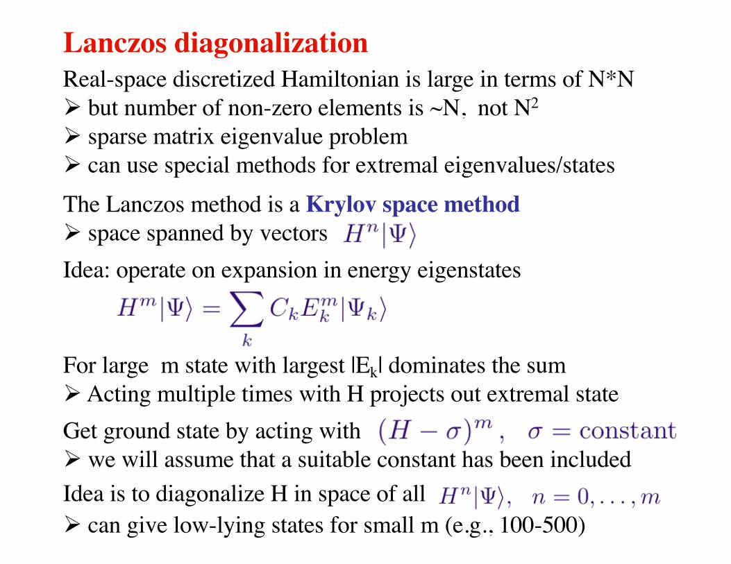
Lanczos diagonalizationReal-space discretized Hamiltonian is large in terms of N*NØ but number of non-zero elements is ~N, not N2
Ø sparse matrix eigenvalue problemØ can use special methods for extremal eigenvalues/statesThe Lanczos method is a Krylov space methodØ space spanned by vectors Idea: operate on expansion in energy eigenstates
For large m state with largest |Ek| dominates the sumØActing multiple times with H projects out extremal stateGet ground state by acting withØ we will assume that a suitable constant has been includedIdea is to diagonalize H in space of allØ can give low-lying states for small m (e.g., 100-500)
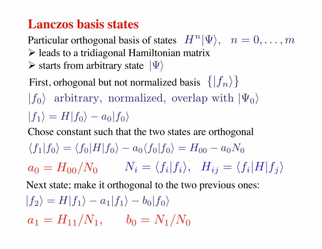
Lanczos basis statesParticular orthogonal basis of statesØ leads to a tridiagonal Hamiltonian matrixØ starts from arbitrary stateFirst, orhogonal but not normalized basis
Chose constant such that the two states are orthogonal
Next state; make it orthogonal to the two previous ones:
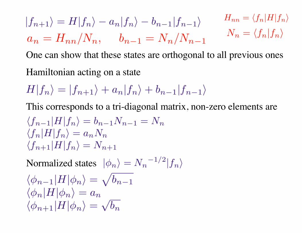
One can show that these states are orthogonal to all previous ones
Hamiltonian acting on a state
This corresponds to a tri-diagonal matrix, non-zero elements are
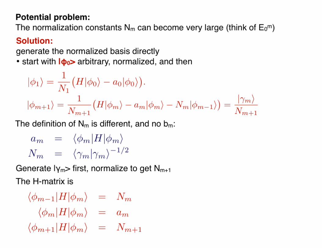
Normalized states
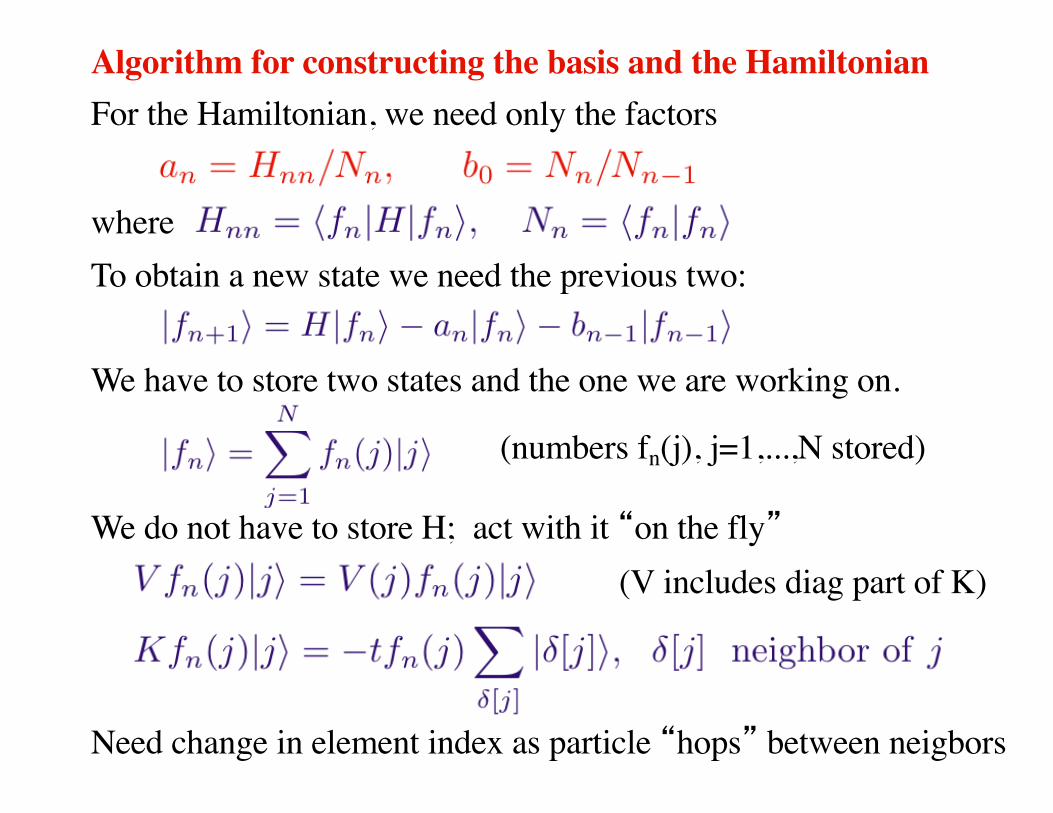
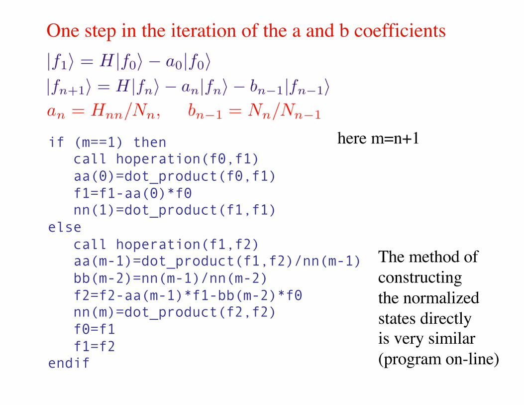
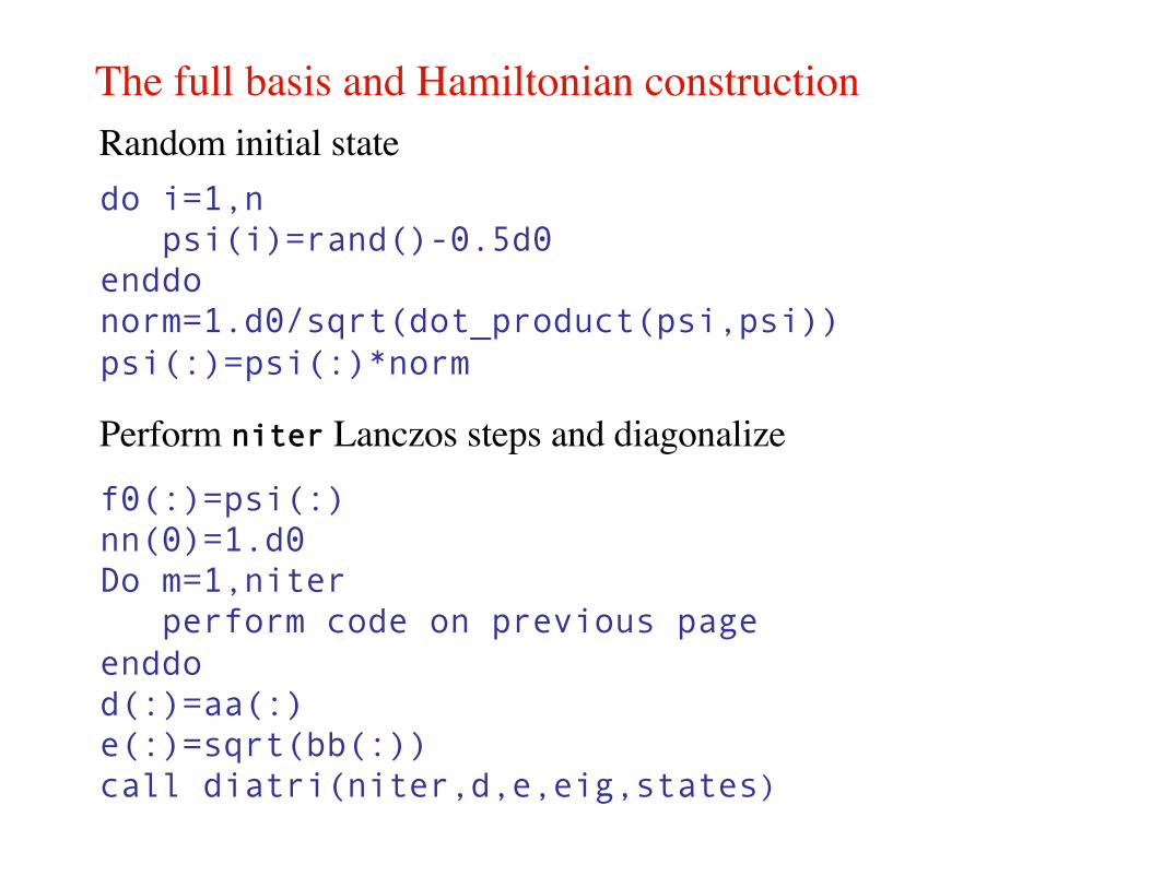
Algorithm for constructing the basis and the HamiltonianFor the Hamiltonian, we need only the factors
where To obtain a new state we need the previous two:
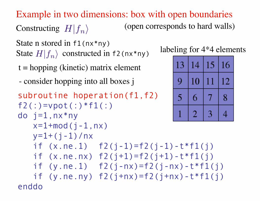
We have to store two states and the one we are working on.
We do not have to store H; act with it “on the fly”
(numbers fn(j), j=1,...,N stored)
Need change in element index as particle “hops” between neigbors
(V includes diag part of K)
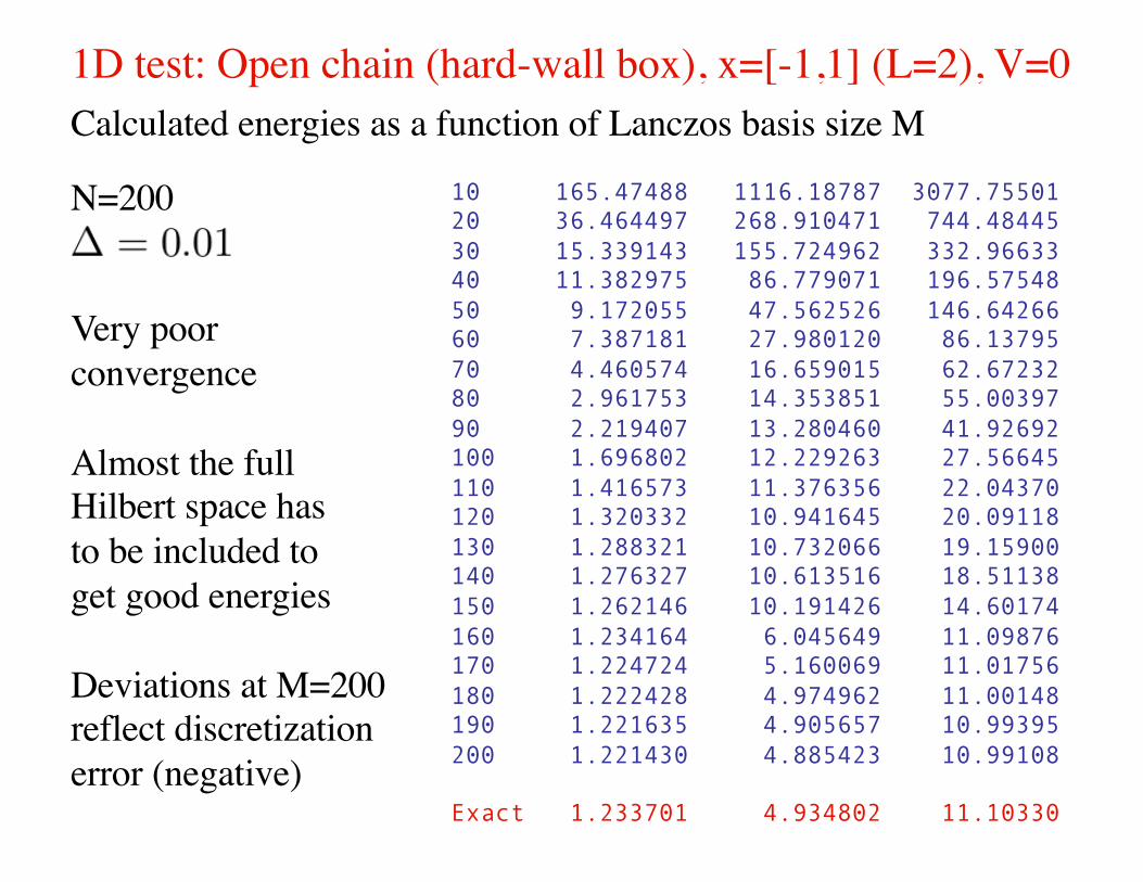
1D test: Open chain (hard-wall box), x=[-1,1] (L=2), V=0Calculated energies as a function of Lanczos basis size M
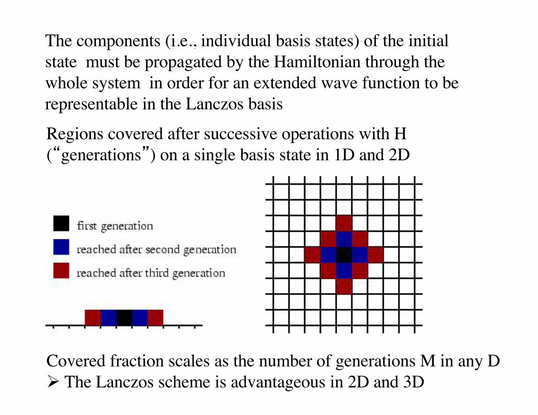
The components (i.e., individual basis states) of the initial state must be propagated by the Hamiltonian through the whole system in order for an extended wave function to be representable in the Lanczos basisRegions covered after successive operations with H (“generations”) on a single basis state in 1D and 2D
Covered fraction scales as the number of generations M in any DØ The Lanczos scheme is advantageous in 2D and 3D
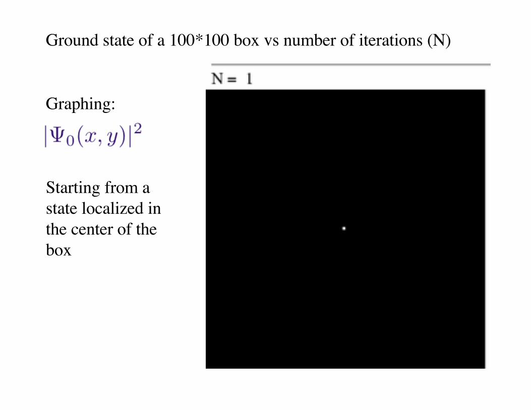
Ground state of a 100*100 box vs number of iterations (N)
Starting from astate localized inthe center of thebox
Graphing:
Ground state of a 100*100 box vs number of iterations (N)
Starting from arandom state
Graphing:
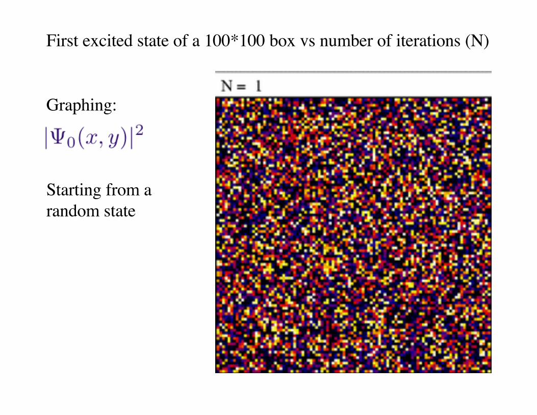
First excited state of a 100*100 box vs number of iterations (N)
Starting from arandom state
Graphing:
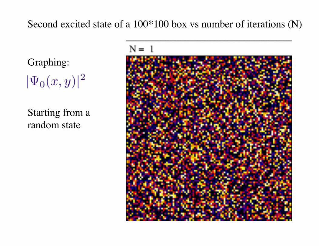
Second excited state of a 100*100 box vs number of iterations (N)
Starting from arandom state
Graphing:
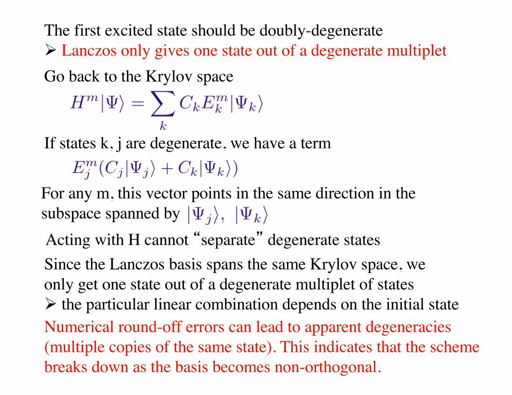
The first excited state should be doubly-degenerateØ Lanczos only gives one state out of a degenerate multipletGo back to the Krylov space
If states k, j are degenerate, we have a term
For any m, this vector points in the same direction in thesubspace spanned by Acting with H cannot “separate” degenerate statesSince the Lanczos basis spans the same Krylov space, weonly get one state out of a degenerate multiplet of statesØ the particular linear combination depends on the initial stateNumerical round-off errors can lead to apparent degeneracies(multiple copies of the same state). This indicates that the schemebreaks down as the basis becomes non-orthogonal.
Example in two dimensions: box with open boundaries
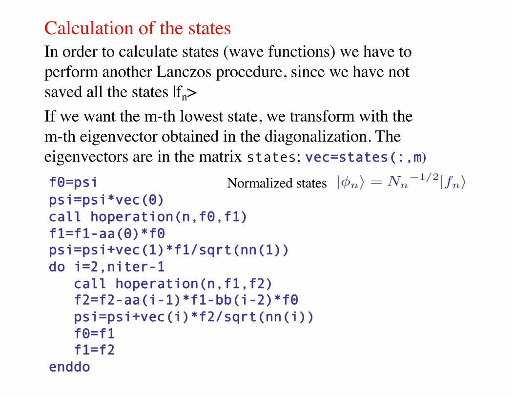
Calculation of the statesIn order to calculate states (wave functions) we have to perform another Lanczos procedure, since we have not saved all the states |fn>If we want the m-th lowest state, we transform with them-th eigenvector obtained in the diagonalization. The eigenvectors are in the matrix states; vec=states(:,m)