Land Use Modeling in Recursively-Dynamic GTAP Framework*

by

Alla Golub1, Thomas W. Hertel2, and Brent Sohngen3

GTAP Working Paper No. 48 2008

1 Center for Global Trade Analysis (GTAP), Purdue University. Corresponding author. Email:

golub@purdue.edu 2 Center for Global Trade Analysis (GTAP), Purdue University. Email: hertel@purdue.edu 3 The Ohio State University. Email: sohngen.1@osu.edu

*Chapter 10 of the forthcoming book Economic Analysis of Land Use in Global Climate Change Policy, edited by Thomas W. Hertel, Steven Rose, and Richard S.J. Tol

2

LAND USE MODELING IN RECURSIVELY-DYNAMIC GTAP FRAMEWORK

Alla Golub, Thomas W. Hertel, and Brent Sohngen

Abstract

The goal of this work is to investigate land-use change at the global scale over the long run – particularly in the context of analyzing the fundamental drivers behind land-use related GHG emissions. For this purpose, we identify the most important drivers of supply and demand for land. On the demand side, we begin with a dynamic general equilibrium (GE) model that predicts economic growth in each region of the world, based on exogenous projections of population, skilled and unskilled labor and technical change. Economy-wide growth is, in turn, translated into consumer demand for specific products using an econometrically estimated, international cross-section, demand system that permits us to predict the pattern of future consumer demands across the development spectrum. This is particularly important in the fast-growing, developing countries, where the composition of consumer demand is changing rapidly. These countries also account for an increasing share of global economic growth and greenhouse gas emissions. Consumer demand is translated into derived demands for land through a set of sectoral production functions that differentiate the demand for land by Agro-Ecological Zone (AEZ). The paper devotes considerable attention to modeling the supply of land to different land-using activities in the economy. We address the issue of land mobility across different uses via sequence of successively more sophisticated models of land supply, beginning with a model in which land is perfectly mobile and undifferentiated, and ending with one in which land mobility across uses is governed by a nested Constant Elasticity of Transformation function. A soft link between our GE model and an intertemporal forestry model is included for better representation of forestry sector in GE model. To reflect the real world fact that deforestation represents an important source of land supply in the face of high demand, we also introduce the possibility of conversion of unmanaged forest land to land used in production. This is treated as an investment decision whereby new land is accessed only when present value of returns on land in a given region is high enough to cover the costs of accessing the new land. In equilibrium, the supply of land to each land-using activity adjusts to meet the derived demand for land. A set of projections for the long run supply and demand for land obtained with this model is a useful input to improving our understanding of land-related GHG emissions in the future. JEL codes C68, R14, Q24 Keywords: land use, climate change policy, baseline, general equilibrium, agro-ecological zones

3

Table of Contents 1. Introduction and Motivation .........................................................................................5 2. Modeling Framework and Baseline Assumptions ........................................................8 Dynamic General Equilibrium Model ..........................................................................8

Structure of Consumer Demand ...................................................................................9 Production Structure ...................................................................................................12 Baseline Assumptions ................................................................................................15

3. Issues in Modeling the Supply of Land ......................................................................17

Heterogeneity of Land ................................................................................................17 Access to New Lands .................................................................................................23

4. Analysis ......................................................................................................................27

Baseline ......................................................................................................................28 Determining the Relative Importance of Alternative Supply-side Specifications .....33

5. Summary and Evaluation ...........................................................................................41 6. References ..................................................................................................................49

4

List of Tables Table 1. Beginning, and projected end-of-period budget shares, assuming constant prices, based on exogenous income and population growth in the baseline ....53

Table 2. Annual Average Total Factor Productivity Growth Rates in Agriculture and Forestry Sectors .........................................................................................54

Table 3. Land earnings by sector and AEZ for 11 regions of the model .......................55 Table 4. Access Cost Function Parameters ....................................................................56 Table 5. Projected Growth Rates in Consumption and Production of Crops, Ruminants and Forestry, from 1997 to 2025 ...................................................56 Table 6. Projected Global and Market Annual Average Percent Changes in Prices of Output in Land Using Sectors Relative, from 1997 to 2025 ............57 Table 7. Access Rates ....................................................................................................58 Table 8. Value of Land and Access of New Lands ........................................................59 Table 9. Share of Accessible Forests to Total Land Employed in Production in the Initial Period ...............................................................................................59 Table 10. Cumulative Growth Rates in Demand for Land in Land Using Sectors..........60 Table 11. Main Features of Six Consecutive Models of Land Supply ............................60 Table 12a. Cumulative Growth Rates in Consumption of Crops, Ruminants and Forestry, Projected with 6 Consecutive Models ..............................................61 Table 12b. Cumulative Growth Rates in Production of Crops, Ruminants and Forestry, Projected with 6 Consecutive Models ..............................................62 Table 13. Cumulative and Annual Growth Rates in Land Rents in Crops, Ruminants and Forestry ..................................................................................63 Table 14a. Cumulative Growth Rates in Demand for Land in Agriculture and Forestry ..64 Table 14b. Cumulative Growth Rates in Demand for Land in Crops and Ruminants ......65 List of Figures Figure 1. Managed forests as share of initial total forestland .........................................66 Figure 2a. Revenue Share Weighted Changes in Land Used in Crop Sector in a given AEZ*country ...................................................................................67 Figure 2b. Revenue Share Weighted Changes in Land Used in Ruminants Sector in a given AEZ*country ..........................................................................................67 Figure 2c. Revenue Share Weighted Changes in Land Used in Forestry Sector in a given AEZ*country ..........................................................................................68

Appendices Table A1. Aggregation of GTAP regions ................................................................................... 69

Table A2. Mapping between 17 produced and 10 consumed goods ................................69

5

LAND USE MODELING IN RECURSIVELY-DYNAMIC GTAP FRAMEWORK

Alla Golub, Thomas W. Hertel, and Brent Sohngen

1. Introduction and motivation

Changes in land use and land cover represent an important driver of net greenhouse gas (GHG)

emissions and are a key part of any long run GHG emissions scenario. Currently, agricultural

activities generate the largest share, 58%, of the world’s anthropogenic non-CO2 emissions (84%

of nitrous oxide (N2O) and 47% of methane (CH4)) and make up roughly 14% of all

anthropogenic greenhouse gas emissions (U.S. Environmental Protection Agency (US EPA),

forthcoming).1 At the same time, forestry offers considerable scope for carbon sequestration; yet

most models of climate change policy have thus far failed to fully take into account the role of

land use and land use change in determining changes in net GHG emissions as a result of

mitigation efforts. A large part of the problem has been the difficulty in appropriately modeling

the derived demand and supply for land in the long run. Hence the focus of this chapter.

In this work, the GTAP-Dyn (Ianchovichina and McDougall, 2001) dynamic general

equilibrium (GE) model of the global economy is modified and extended to investigate long-run

land-use change at the global scale. For this purpose, we identify the most important drivers of

supply and demand for land from 1997 to 2025. A better understanding of this interaction is

critical for the long run analyses of the environmental implications of land use and land use

change. We begin with an analysis of consumption behavior in the presence of economic growth,

since it is the demand for food and forestry products that drives much of the long run demand for 1 Agricultural sources of NO2 emissions include manure management, agricultural soils, field burning of agricultural residues, and prescribed burning of savannas. These activities are also sources of CH4 emissions. Main sources of CH4 in agriculture are manure management and rice cultivation.

6

land. Depending on the location of this demand, and the nature of the production undertaken on

this land, the pattern of international demands can have important implications for the emissions

of greenhouse gases from agriculture and forestry. We then turn to an analysis of the scope for

accessing new lands, and converting land from forestry to agriculture, and vice versa.

Examples of other large scale simulation models that investigate the tradeoffs between

different land use decisions are the Forest and Agriculture Sectors Model (FASOM) of Adams et

al. (1996), the Future Agricultural Resource Model (FARM) of Darwin (1995), D-FARM of

Ianchovichina et al. (2001), and the modified global trade and environment model (GTEM) of

Ahammad and Mi (2005). FASOM is a dynamic optimization model that explores allocation of

land between agriculture and forestry in the United States. FARM (Darwin, 1995) is a global

computable general equilibrium model which is a modified version of the GTAP model. In this

model, land is differentiated in six classes, distinguished by the length of the growing season.

Land owners allocate land among uses on the basis of a constant elasticity of transformation

(CET) function. D-FARM (Ianchovichina et al., 2001) extends the FARM model to allow

dynamic adjustments over time. The model of Ahammad and Mi (1996) is an extension of

GTEM to allow modeling land use changes and associated GHG emissions. Following Darwin

(1995), it differentiates land by the length of growing season and utilizes a CET function to

model allocation of land across uses. Different from FARM, the allocation of land is a multistage

decision process, governed by nested CET functions.

Building on the existing approaches to modeling land use, particularly that of FARM, D-

FARM and GTEM, the contribution of this chapter is three-fold. First of all, we incorporate into

a recursive dynamic general equilibrium model, a very flexible, non-homothetic demand system

that permits changes in the patterns of consumer demand to determine the long run derived

7

demand for land. Second, in response to our initial model projections, we incorporate a soft link

between the GE model and forestry model for better representation of forestry sector in GE

model. Third, we introduce an investment decision by which land owners consider the

conversion of unmanaged forests to commercial forestry or agricultural land.

For purposes of this work, the standard demand structure of GTAP –Dyn model is

modified. We introduce an international cross-section, demand system that permits us to predict

the pattern of future consumer demands, particularly in the fast-growing, developing countries

that account for an increasing share of global economic growth – as well as greenhouse gas

emissions. The production structure of land using sectors and specification of land supply are

also modified. The later issue is addressed via a sequence of successively more sophisticated

models of land supply. We start from assumption that land is perfectly mobile across uses and

then gradually restrict mobility of land, introducing Agro-Ecological Zones (AEZs) and nested

model of land supply. Our approach is motivated by the findings in the existing literature on land

use that land quality and land rents play an important role in determining how landowners

allocate land among uses (see Choi et al. (2006) for a literature review).

While the introduced features offer what appears to be a quite realistic representation of

the individual determinants of land supply and demand, the resulting baseline land rental changes

in forestry and grazing appear excessively large. Further analysis suggests that this is driven by

the following limitations of the model: the lack of forestry input-augmenting productivity growth

in forestry processing sectors and, to some extent, by the absence of unmanaged land that can be

brought into commercial production when the derived demand for land is high. Therefore, these

issues are subsequently addressed.

8

Any decision regarding forestry production is always a forward looking decision. Unlike

crops and, to some extent, livestock, growing a tree takes a very long period of time, and optimal

decisions regarding the timing of forestry harvesting could be modeled only in a forward looking

framework. To improve the representation of the forestry sector in a dynamic recursive model,

like GTAP-Dyn, a link with forestry dynamic forward looking model is required. We iterate

between GTAP-Dyn and Global Timber Model of Sohngen and Mendelson (2006) to determine

forestry input-augmenting productivity growth in forestry processing sectors in GTAP-Dyn.

Using the rate of unmanaged forest access predicted by the Global Timber Model, we introduce

the possibility of conversion of unmanaged forest land to land used in production when demand

for cropland, pasture or commercial forestland is high, and land rents are high enough to cover

cost of access of unmanaged land.

The chapter is organized in five sections. The modeling framework, structure of

consumer demand and production sectors, as well as baseline assumptions are discussed in

section two. Sections three is devoted to various issues in modeling land supply. The projected

baseline derived demand for land and comparison of alternative supply-side specifications are

analyzed in section four. Summary of the results and discussion of limitations are presented in

section five.

2. Modeling Framework and Baseline Assumptions

Dynamic General Equilibrium Model

Projections of future global economic activity are undertaken using a modified version of the

dynamic GTAP model (Ianchovichina and McDougall, 2001). The dynamic GTAP model is a

multi-sector, multi-region, recursive dynamic applied general equilibrium model that extends the

9

standard GTAP model to include international capital mobility, endogenous capital

accumulation, and an adaptive expectations theory of investment. The distinguishing feature of

the model is its disequilibrium mechanism for determining the regional supply of investments.

This mechanism consists of adjustment of the expected rate of return toward actual rate of return

within each region and adjustment of the regional expected rate of return toward the global rate

of return to capital. These lagged adjustment mechanisms, as well as the mechanism determining

the composition of capital and allocation of wealth are parameterized according to econometric

estimation documented in Golub (2006).

In order to facilitate long run projections of the sort desired for climate change policy

analysis, the GTAP-Dyn has been modified. The usual assumption of fixed savings rates has the

unwelcome implication that as economies with high savings rates, like China, grow, there is a

“glut of global savings” and, as a result, investments and capital in the world. Because of

excessive amount of capital, rates of return to capital are not stationary in the long run.

Therefore, in this work we adopt a new approach to the evolution of savings over time (Golub

and McDougall, 2006) in which the theoretical structure of GTAP-Dyn is modified such that the

wealth to income ratio in each region is stabilized at region specific level. Thus the savings rate

becomes an endogenous function of the ratio of wealth to income. This approach is motivated by

the balanced growth theory which implies that in steady state, regional income, wealth and

savings share the same rates of growth.

Structure of Consumer Demand

The specification of consumer demand is critical for any long run GE growth model. As

economies become richer and per capita incomes grow, the income elasticities of demand will

10

determine demands for different products. These changing consumer demands, together with

resource constraints will translate into changing production patterns. Thus, specification of

consumer demand is an important issue in assessing climate change policies, since it influences

the scale and location of each production activity and, hence, associated GHG emission levels.

For example, changes in demands for staple crops, livestock products, processed foods and

forestry products will determine changes in derived demand for land in each of these activities,

land cover, non-carbon dioxide GHG emissions and forest carbon sequestration.

In the choice of demand system for our analysis we follow Yu et al. (2002) where the

properties of a demand system desirable for long run projections are identified. First, the demand

system should be internationally comparable to be used in the global economy projections.

Second, the demand system should be consistent with economic theory and should satisfy usual

economic restrictions such as adding-up, symmetry and homogeneity. Consistency with

economic theory guarantees that budget shares stay non-negative and sum to one in the long run

projections involving very large changes in income. Third, the utility function underlying the

demand system should be non homothetic to allow changes in the budget shares as income rises.

This is especially important for projections of demand for staple food for which budget shares

declines as income rises. Finally, the demand system should be very flexible and allow

adjustment not only in average budget shares, but also adjustment in marginal budget shares, i.e.

fraction of extra dollar spent on food. The adjustment in marginal budget shares is necessary for

a non-monotonic path of income elasticities. This permits, for example, income elasticities of

staple foods − necessities at low income level − to fall as income rises.

As recommended by Yu et al., we adopt an implicit directly additive demand system

(AIDADS) developed by Rimmer and Powell (1996). The AIDADS demand system is rank 3,

11

meaning that it is very flexible in its ability to represent the non-homothetic demand for

consumer goods. Furthermore, it has been shown to outperform competing demand systems in

the prediction of observed demands – particularly demand for food – across a wide range of

income levels (Cranfield et al., 2003). From the point of view of determining the long run

demand for land in crops, livestock and forestry, the most important feature of this demand

system is the fact that the average and marginal budget shares for these (and other) products

varies with the level of real, per capita income.

We adopt the AIDADS estimates offered by Reimer and Hertel (2004). We subsequently

calibrate the model to each of the 11 regions in our aggregation2 using the approach outlined by

Golub (2006). With a complete demand system in hand for each region in our aggregation, we

are in a position to project the pattern of per capita, national consumer demands in all 11 regions,

in the year 2025. The impact of income growth on the pattern of consumer expenditure can be

nicely illustrated by shocking income per capita by growth in this variable over the 1997-2025

period assuming constant prices for all goods and services. In this illustration, projections of per

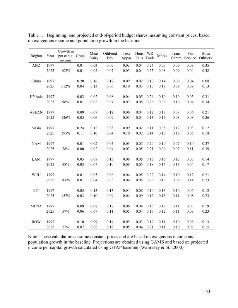
capita income are exogenous and based on the GTAP baseline (Walmsley et al., 2000). Table 1

reports the 1997 and projected 2025 expenditure shares for 10 aggregate commodities in the

AIDADS system at constant prices in each of the 11 regions. Note that these shares vary

relatively little for Australia and New Zealand (ANZ), High Income Asia (HYAsia), North

America (NAM) and Western Europe (WEU) − the high income and slow growing (in terms of

per capita income) regions. These regions are characterized by slightly increasing budget shares

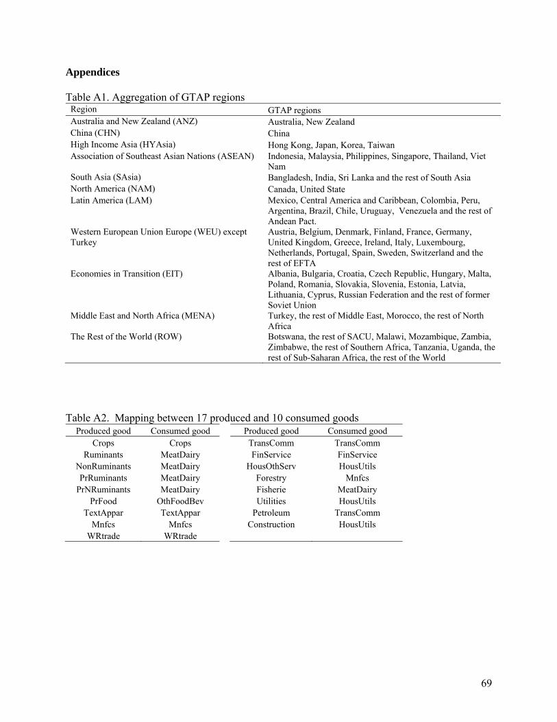
for services (wholesale, financial, housing and others) and corresponding decreasing budget 2 The choice of aggregation scheme is driven by our focus on the derived demand for land due to income growth. The 78 regions of the GTAP 5.4 data base (Dimaranan and McDougall, 2002) are aggregated to 11 regions according to the mapping reported in Appendix Table A1. This aggregation, while parsimonious, represents a broad spectrum of income levels and development across regions.

12

shares for other commodities. In contrast, budget shares in low income and rapidly growing

regions, represented by China and South Asia (SAsia) in our aggregation, change quite a bit over

the projections period. In these regions budget shares for food products decline significantly,

especially in China. The share spent on textile and apparel products declines slightly, and shares

spent on manufactured products and different types of services grow quite strongly over the

baseline. The other five regions in our aggregation are relatively poor, but have more moderate

(ASEAN, Economies in Transition (EIT)) or low (Latin America (LAM), Middle East and North

Africa (MENA), Rest of the World (ROW)) per capita growth rates. While budget shares spent

on food products are large initially, they decline very little over the 1997-2025 period. Similar to

high income slow growing regions, these regions are characterized by slightly growing budget

shares for services and small decline in budget shares for other commodities.

Of course all of these demands represent consumer demands. Not land demands. To get

to the derived demand for land, we must first consider how these consumer demands are met.

This takes us to the supply side of the model – in particular the sectoral production functions.

Production Structure

The supply side of this model begins with the standard GTAP model (Hertel, 1997) production

functions. These are constant returns to scale, nested CES functions, which first combine primary

factors into composite value-added, and imported and domestic intermediate inputs into

composite intermediates, before aggregating these composites into an aggregate output. Тhere

are 17 production sectors in each region. The 17 produced goods are then combined into 10

consumed goods, according to the mapping reported in Appendix Table A2, using fixed

proportions. Some of the 10 consumed goods are composites of several produced goods. For

13

example, the consumed composite MeatDairy consists of ruminants, non-ruminants, processed

ruminants and processed non-ruminants. While consumed quantities of the composites grow at

the same rate because of fixed proportion assumption, prices of the composites can diverge as

economy grows and relative prices change.

In keeping with our interest in the derived demand for land, we modify the standard

GTAP production structure in the forestry, crops and livestock sectors. In the forestry sector, we

allow for effective substitution between land and other value added inputs (labor and capital) at

the national level, based on predictions from the Global Timber Model (Sohngen and

Mendelsohn, 2006). Specifically, we observe that changes in management intensity permit

substantial changes in forestry output per unit of land. Accordingly, we increase the elasticity of

substitution between land and other value added inputs from 0.2 − standard GTAP model

magnitude of the elasticity of substitution in value added for natural resource extraction sector −

to 1.0, a value suggested by the work reported by Hertel et al. (this volume) where the authors

explore the sensitivity of management input to carbon price changes. Note that Ronneberger et

al. (this volume) also increased this substitution elasticity to assure convergence between

economic and biophysical models in their coupling procedure.

In the livestock sectors we permit producers to vary the intensive margin of ruminant

livestock production. In particular, we permit substitution amongst feedstuffs, and between

feedstuffs and land.3 Therefore, as land rents rise over the baseline projections period, provided

TFP growth in agriculture is sufficient to keep crop prices flat or declining (as has been the case

historically), producers make greater use of feedlots and intensify their livestock production

practices. This phenomenon has proven to be very important in the evolution of livestock

3 We set the elasticities of substitution between feed and land, and between feedstuffs to 0.75.

14

production – both in the US and overseas (e.g., China) and is captured in our model via the

substitution of purchased feedstuffs for land in the national production function for livestock.

In crop production, we allow substitution between land and fertilizers to reflect the fact

that producers will use more fertilizers to increase yields per hectare as land prices rise under the

pressure of increasing derived demand for land. In the choice of the elasticity of substitution, we

follow the approach outlined in Keeney and Hertel (2005).4 The region specific elasticities of

substitution between value added composite and intermediate inputs are set according to the

values of the Allen partial elasticity of substitution between land and purchased inputs reported

in OECD (2001). Then, using Allen partial elasticities of substitution between land and other

farm-owned inputs, also reported in OECD (2001), we calibrate elasticity of substitution among

value added inputs.

As household income rises over the projections period, consumers demand not only a

greater quantity of food, but also higher quality food. A recent study of China suggests that

“…the demand for quantity diminishes as income rises, and the top tier of Chinese households

appear to have reached a saturation point in quantity consumed of most food items. Most

additional food spending by this emerging middle class of consumers is spent on higher quality

or processed foods and meals in restaurants.” (Gale and Huang, 2007). These current trends in

China repeat ones observed earlier in higher per capita income countries. The fraction of the

average consumer dollar spent on food which actually goes to farmers has been continually

declining over the past century (Wohlgenant (1989); Economic Research Service (ERS), US

Department of Agriculture (USDA) (2006)). For this reason, we introduce the possibility of

4 Unlike Keeney and Hertel (2005), we do not model substitution among non-farm purchased intermediate inputs in crops.

15

substitution between farm and marketing inputs in food processing – in effect allowing the food

marketing system to boost the non-agricultural content of food products. For the aggregation

used in our land use model, three sectors seem suitable for introduction of this type of

substitution: processed ruminants (PrRuminants), processed non ruminants (PrNRuminants) and

processed food (PrFood). The values for these elasticities of substitution are taken from

Wohlgenant (1989) and range from 0.35 for pork to 0.96 for dairy products.5

Baseline Assumptions

The starting point of our simulation is the world economy in 1997, as depicted in the GTAP v.5.4

data base. In our simulations from 1997 to 2025, labor force, population and productivity growth

are all exogenous to the model. Projections of labor force (skilled and unskilled labor) growth

rates for 1998 – 2025 are taken from Walmsley et al. (2000). The historical real GDP and

population growth rates for 1998-2004 period are constructed using World Development

Indicators database. The real GDP path for 2005 − 2025 is driven by our assumptions about

productivity growth in various sectors of the economy. Productivity growth rates in non-land

using sectors are based on our assumptions about economy-wide labor productivity growth in

each region, adjusted for productivity differences across sectors using estimates reported in Kets

and Lejour (2003). For detailed description of the productivity growth in non-land using sectors

the reader is referred to Hertel et al. (2006).

There are two land-using sectors: agriculture and forestry. Agriculture, in turn, combines

crops, ruminants and non-ruminants. While non-ruminants are included in the discussion here, in 5 A large part of our processed food sector (PrFood) is processed fruits and vegetables. Wohlgenant (1989) excludes this commodities from the reported results"...because of the wrong sign on the farm output variables". As a proxy for the elasticity of substitution in the processed food sector, we use the elasticity for “Fresh Vegetables” which equals 0.54.

16

the model the use of land by this sector is set to zero to reflect the fact that production of non-

ruminants does not involve grazing land and is largely undertaken in confined settings, that are

more nearly akin to factories than farms. For the three agricultural sectors, the projected

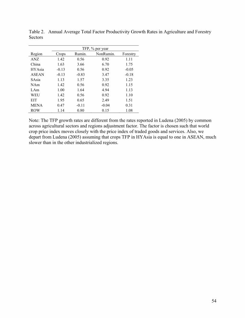
productivity growth rates are taken from Ludena (2005). 6 These productivity growth rates take

into account the productivity of all inputs, not just value-added. In the absence of better

information, productivity growth rates in forestry are assumed to be equal to the average of

productivity growth rates in crops and ruminants, weighted by the share of their output in total

output of crops and ruminants. This is a “neutral” assumption that does not have an affect on the

allocation of land between agriculture and forestry. The annual geometric average productivity

growth rates in agriculture and forestry sectors are reported in Table 2.

It remains to discuss how we model technical change in forestry processing sectors − a

key factor in determining the derived demand for land used in the forestry sector. According to

our estimates, real output in the forest products industry in the U.S. increased by 3.8% per year

since 1977, whereas the quantity of industrial roundwood harvested in the U.S. increased only by

1.2% per year over the similar period (Haynes, 2003). According to Haynes (2003), in United

States production of wood, paper, and paperboard products per unit of industrial roundwood

input increased by 35 percent in the past 50 years. This suggests that there has been strong forest

input-augmenting technical change in manufacturing and other sectors.

Because this technical change in the forest-using sectors is not directly observable and is

difficult to estimate, we adopt an indirect approach to this problem. We iterate between the

6 In our baseline, we augment productivity growth rates in the three agricultural sectors, reported in Ludena (2005), by a common across regions factor “tfp-agriculture”, which is chosen such that world crop price index moves closely with the price index of traded goods and services. Without such adjustment, the crop prices could rise by an implausible amount over the projection period, which would be in sharp contrast with historical evidence on falling crop prices. As it turns out, this adjustment factor is very small, and could be dropped altogether with little change in the findings.

17

GTAP-Dyn model and the Global Timber Model of Sohngen and Mendelsohn (2006) to

determine the relative price of global forestry output. Given baseline GDP, population and

AIDADS income elasticities, determining baseline timber consumption path, the Global Timber

Model projects global price of forestry. In GTAP-Dyn, we target this price by endogenizing

global forestry input-augmenting technical change in forestry processing which plays a key role

in determining the long run demand for forest land, and hence land rents (see next section 4 for

details).

3. Issues in modeling the supply of land

The focal point of this chapter is the way in which land supply is modeled in general equilibrium,

and the implications for the long run use of land in the context of a baseline scenario. We

consider two key aspects of land supply in particular: heterogeneity of land, and access to new

lands. In this section we outline the conceptual issues associated with each of these challenges.

We will then explore their implications in the context of a long run baseline for land use.

Heterogeneity of Land

We will explore the structure of the land market by employing a sequence of successively more

complex representations of land supply, and investigating their implications for future patterns of

land rents and land use. A natural place to begin with is the naïve assumption that land is like

labor and capital inputs in the GE model – homogeneous and perfectly mobile across crops,

livestock and forestry in the medium run. In this case, there is a single land rental rate per region

18

that is equated across all uses.7 Therefore, when the derived demand for land in one sector (e.g.,

forestry) increases, a substantial shift in land is required in order to re-equilibrate the system. A

model operating under such assumptions will overstate the potential for heterogeneous land to

move across uses.

A natural way to overcome this heterogeneity problem is to disaggregate the land

endowment –much as is done with labor (e.g., disaggregating into skilled and unskilled labor) in

CGE models. We do this by bringing climatic and agronomic information to bear on the problem

– introducing Agro-Ecological Zones (AEZs) data base (Lee et al., 2005).8 This data base

enhances the standard GTAP global economic data base by disaggregating land endowments into

18 AEZs. These AEZs represent six different lengths of growing period (6 x 60 day intervals)

spread over three different climatic zones (tropical, temperate and boreal). Following the work of

the Food and Agriculture Organization (FAO) and International Institute for Applied Systems

Analysis (IIASA), the length of growing period depends on temperature, precipitation, soil

characteristics and topography (see also Part II of this book). This approach evaluates the

suitability of each AEZ for production of crops, livestock and forestry based on currently

observed practices, so that the competition for land within a given AEZ across uses is

constrained to include activities that have been observed to take place in that AEZ. Indeed, if two

7 In the standard GTAP model, land is assumed not to move between agriculture and forestry, and it is imperfectly mobile within agriculture. 8 Another modification of the standard GTAP data base undertaken in this work is an adjustment of the cost share of land in forestry sector. In the standard GTAP data base, the land share in forestry is unrealistically small – about 7% of value added. This share of land in forestry was been chosen to give a reasonable degree of aggregate supply response in the forestry sector (see Hertel and Tsigas, 2002). However, it has no firm basis in the direct measurement of land rents. This could be improved by combining estimates of per hectare land rents in forestry with Global Timber Market and Forestry Data and forestry hectares estimates obtained with Global Timber Model (Sohngen et al.1999). Gouel (2006) used this method to calculate the world average cost share of land in forestry. We use his estimate – world average cost share of 0.39 – to adjust the cost share of land in forestry in the data base.

19

uses (e.g., citrus groves and wheat) do not presently appear in the same AEZ, then they will not

compete in the land market.

From the point of view of the general equilibrium model, the key dimension of the land

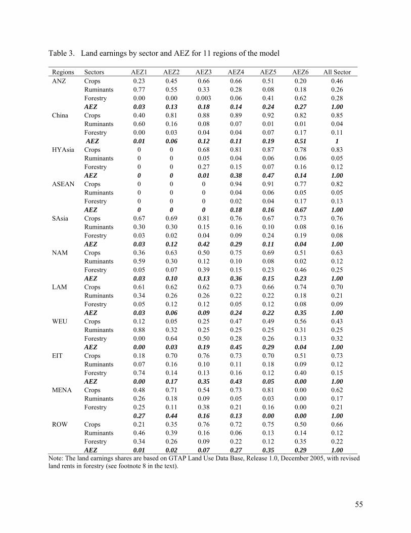
use data base is the economic importance of land in each AEZ and each activity. Table 3

summarizes land rental shares for cropping, livestock and forestry activities, within 6 AEZs, in

the 11 regions (we aggregate over the climate dimension of the AEZs for purposes of this

chapter). Thus, the shares within any given column sum to one across uses, for any given

AEZ/region. The boldface row in each regional block reports the share of total land rents in a

given AEZ in total regional land rents (summed across all AEZs).

From this table, we see that AEZ1 (very short growing period) in ANZ, WEU and ROW

is dominated by livestock grazing activity, while extensive cropping dominates in South Asia,

Latin America and MENA. In AEZ1 forestry is relatively large component of land rents only in

EIT. Cropping activity tends to be economically dominant in AEZ2 for China, South Asia,

NAM, LAM, EIT and MENA, forestry is relatively important in WEU, whereas grazing

activities dominate in ANZ. On the other hand, cropping activity dominates in all regions, except

ANZ, in more productive locales: AEZ3 – AEZ6. However, importance of forestry is gradually

rising from AEZ3 to AEZ6 in many regions. And it becomes economically quite important in

AEZ6 (the longest growing period) in ANZ, NAM, EIT and ROW.

It is also important to look at the pattern of land rents within a given country, aggregated

across AEZs (final column of Table 3). Cropping activity dominates ruminants and forestry in

terms of economic value in all regions. In China, cropping activity accounts for an estimated

85% of total land rents in forestry and agriculture. This figure is much lower in Australia/New

Zealand, and Europe. Forestry dominates ruminants in many regions including, China, HYAsia,

20

ASEAN, NAM, WEU, MENA and ROW, while the ruminants sector is economically more

important in SAsia and LAM. Forestry and ruminants are almost equally important, as measured

by estimated land rents, in ANZ and EIT.

Table 3 gives us some insight into the importance of disaggregating AEZs in a particular

region, since the elasticity of land supply to each land using activity depends on these land rent

shares. In the extreme, if the entry for a given activity in a given AEZ is zero, this activity will

not compete in the land market at all. For example, a rise in the price of forest products will have

no impact on the land market in AEZ1 in China. On the other hand, small, but unimportant uses

have more scope to grow than dominant ones. For example, rising beef prices in China will have

a large positive impact on percentage growth of grazing land in AEZ6. By contrast, activities

which already dominate land rents in a given AEZ, such as crops in China’s AEZ4 and AEZ5,

have little room to expand – and the land supply elasticity will be very low. Whereas a rise in

relative crops prices may generate a significant increase in acreage devoted to crops in AEZ1,

there is very little scope for expansion at the extensive margin of the higher AEZs in China. Of

course, the activity/AEZ variation would be much greater if crops were further disaggregated

into paddy rice, cotton, wheat, etc in the model, making the presence of AEZs even more

important.

Despite the rather coarse grouping of land into AEZs, there is still considerable

heterogeneity within these units, and this, in turn, is likely to limit the mobility of land across

uses within an AEZ. In addition, there are many other factors, beyond those reflected in the

AEZs, that limit land mobility. These include costs of conversion, managerial inertia, un-

measured benefits from crop rotation, etc. A natural way to constrain land mobility within an

AEZ is via the Constant Elasticity of Transformation (CET) frontier. This is the approach taken

21

in the standard GTAP model (Hertel, 1997), and it is effective at restricting land mobility.9 The

mobility of land across uses is governed by the CET parameter, or the elasticity of

transformation, which is non-positive. In this specification, the absolute value of the CET

parameter represents the upper bound (in the case of a tiny rental share) on the elasticity of

supply to a given use of land in response to a change in its rental rate. The lower bound on this

supply elasticity is zero (the case of a unitary land rental share). If the CET parameter is close to

zero, then the allocation of land across uses is nearly fixed and unresponsive to changes in

relative returns to land in different activities. If the CET parameter is large in absolute

magnitude, then allocation of land is very sensitive to disparities in relative returns across land

using activities, and land is very mobile across uses.

In a final variant of the land supply model, a nested, multi-stage, optimization structure is

introduced which allows better representation of the land transformation possibilities across uses.

This follows the approach first proposed in Darwin et al. (1995) and then further developed in

Ahammad and Mi (2005). Owners of the particular type of land (AEZ) first decide on the

allocation of land between agriculture and forestry to maximize the total returns from land. Then,

based on the return to land in crop production, relative to the return on land used in ruminant

livestock production, the land owner decides on the allocation of land between these two broad

types of agricultural activities.10 These allocations are governed by CET functions. At each stage

in the decision making process, the CET parameter increases, reflecting the greater sensitivity to

relative returns amongst crops and livestock than between forestry and agriculture – where the

allocation decision can be irreversible in the near term. 9 A key difference between this variant of the model and the standard GTAP model is that land is assumed to be mobile between agriculture to forestry. 10 Currently there is only one crop commodity in the model. Though not modeled in this work, the nested structure can be expanded to allow the allocation of land to various crops.

22

We calibrate the elasticity of transformation of land between agriculture and forestry to

econometric estimates. Based on data for U.S. Midwestern forests, Choi (2004) estimates the

own price supply elasticity of land to forestry to be 0.516. Sohngen and Brown (2006) report an

average land supply elasticity for different types of forests of 1.48. Using initial forestry revenue

shares in total land rents in each AEZ/region, we calibrate the CET transformation parameter

such that initial supply elasticities are in the range between these two econometric estimates.

Specifically, we choose a CET parameter of -1.5 so that the maximum supply elasticity is just

under 1.5. 11 The elasticity between crops and livestock is set to -3 − twice larger by absolute

magnitude, reflecting the relatively easier conversion of crop land to grazing (as opposed to

conversion of agricultural land to forestry and vice versa).

Having introduced AEZs into the model, we must also determine how products produced

on different AEZs compete. The most natural approach would be to have a different activity for

each AEZ/product combination, with the resulting outputs (e.g., wheat) competing in the product

markets. If like products produced on different AEZs are perfect substitutes, then a single price

will prevail. If the production functions are similar, and the firms face the same prices for

nonland factors, then land rents in comparable activities must also move together. This

assumption can be introduced into the model in a variety of ways. The first is to incorporate

separate production functions for each AEZ/product combination. With as many as 6 AEZs, this

results in a great proliferation of sectors and dimensions in the model which is a problem –

particularly for dynamic analysis of global issues. An alternative is to retain a single, national 11 In earlier work by Golub et al. (2006) value of -0.25 for the CET transformation parameter between forestry and agriculture was used. The smaller absolute magnitude assumes less sensitive land supply to changes in relative returns to land. In this work larger parameter is used to reflect new econometric estimates of Sonhgen and Brown (2006). We also think that larger magnitude of the CET parameter is plausible in the long run scenarios − as opposite to static one like in another chapter of this book “The Role of Land Use in Determining the Economy-wide Cost of Greenhouse Gas Abatement” by Hertel et al. − to reflect greater flexibility of land allocation in the long run.

23

production function for each commodity, but to introduce the different AEZs as inputs to this

national production function. With a sufficiently high elasticity of substitution in use,12 the return

to land across AEZs, but within a given use, will move closely together. This approach is taken

here.13

Access to New Lands

The second key issue in land supply that we explore in this chapter has to do with access to new

lands. In North America, 75% of forest lands are estimated to be currently inaccessible, and

therefore not employed in commercial production. In Australia and New Zealand, this figure is

above 90% (Global Timber Market and Forestry Data Project, 2004). This represents a

substantial source of commercial land, some of which could reasonably be expected to come into

use if land rents were to rise sufficiently to bring them into production.

A land owner’s decision to add new land to production possesses the two main features

of an investment decision. First, the conversion of unmanaged land today yields a stream of

future benefits from production undertaken on this land. Second, conversion of unmanaged land

is costly because it requires building roads and other infrastructure. Thus, the initial outlay of

resources required to access the land must be weighed against future benefits. To model access

of unmanaged land as an investment decision, we follow approach described in the Gouel and

Hertel (2006) and briefly summarized here.

The price of land today reflects the present value of future benefits generated by

production activities on this land. In the context of our model, land owner’s benefits from

12 In this model, the elasticity of substitution among AEZs in production is set to 20. 13 See the related discussion in Chapter “The Role of Land Use in Determining the Economy-wide Cost of Greenhouse Gas Abatement” of this book by Hertel et al.

24

holding a land are measured by land rents. With myopic expectations for both the land rents and

the rate of return (the only option available in our recursive dynamic model) the price of land can

be expressed in terms of the present value of ordinary annuity:

LandrentPr

= (1)

where P denotes the price of one hectare of forestland that can be converted to land used by one

of three land using activity, Landrent is the average (across uses) annual land rent generated in a

given period, and r is the net rate of return that investors expect to earn over that same period.14

Because access of new land requires an initial outlay of resources, represented by access costs C,

the net present value of accessing new land is:

LandrentNPV Cr

= − + (2)

The marginal costs of accessing new land are expected to rise as more land is accessed and less

land is left unmanaged, holding prices of production factors fixed or rising.15 The marginal

hectare of land is accessed when net present value of the decision to access is zero, which is

reflected in equality of access cost of the marginal hectare to present value of benefits it

provides:

LandrentCr

= (3)

Thus, the higher land prices generated under pressure from consumer demand for crops,

livestock and forestry attract more unmanaged land into the production process. But, new land is

accessed only when value of land in a region is high enough to cover the costs of access, which

14 The rate of return is net of depreciation, which is zero for land asset. Thus, net rate of return and rate of return on land are equal. 15 The access activity is modeled as a production function, where capital and unskilled labor are production inputs and accessed hectares of unmanaged forests are output.

25

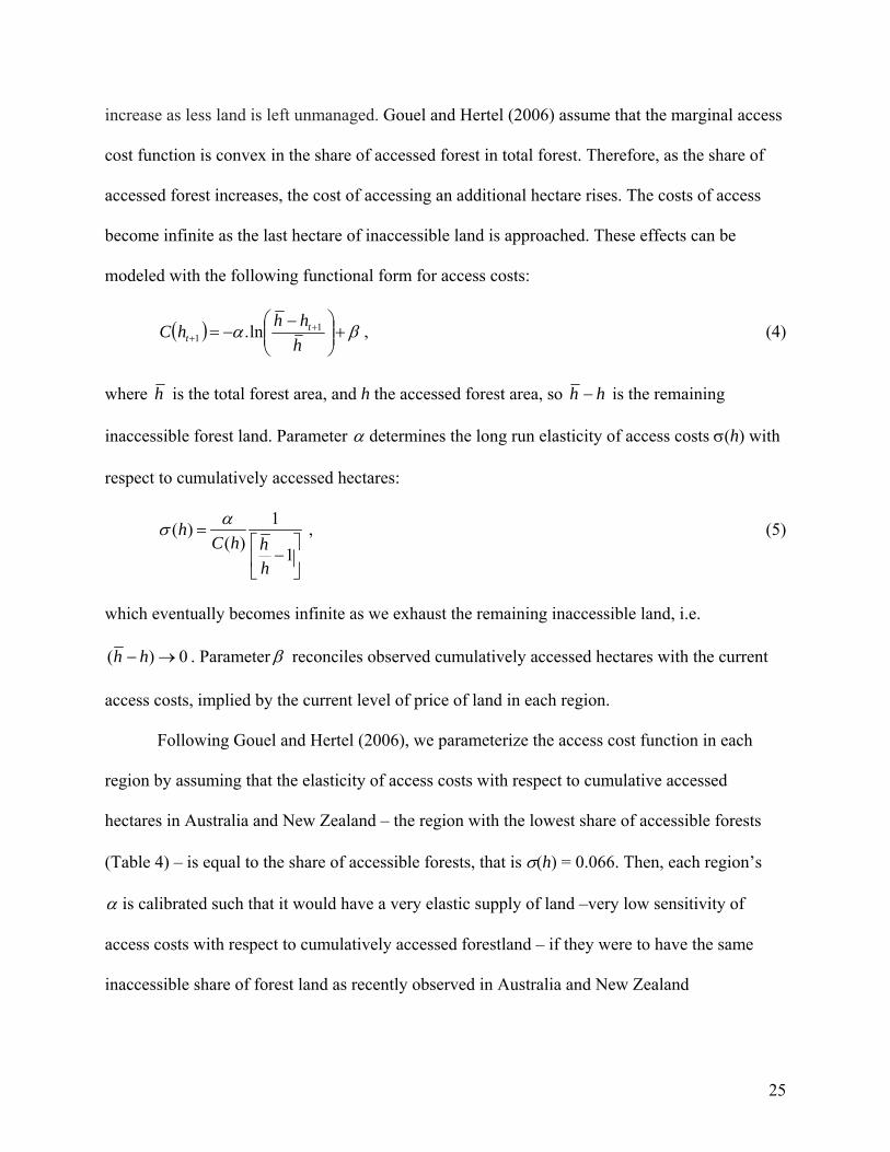
increase as less land is left unmanaged. Gouel and Hertel (2006) assume that the marginal access

cost function is convex in the share of accessed forest in total forest. Therefore, as the share of

accessed forest increases, the cost of accessing an additional hectare rises. The costs of access

become infinite as the last hectare of inaccessible land is approached. These effects can be

modeled with the following functional form for access costs:

( ) βα +⎟⎟⎠

⎞⎜⎜⎝

⎛ −−= +

+ hhhhC t

t1

1 ln. , (4)

where h is the total forest area, and h the accessed forest area, so hh − is the remaining

inaccessible forest land. Parameter α determines the long run elasticity of access costs σ(h) with

respect to cumulatively accessed hectares:

1( )( )

1h

C h hh

ασ =⎡ ⎤

−⎢ ⎥⎣ ⎦

, (5)

which eventually becomes infinite as we exhaust the remaining inaccessible land, i.e.

( ) 0h h− → . Parameter β reconciles observed cumulatively accessed hectares with the current

access costs, implied by the current level of price of land in each region.

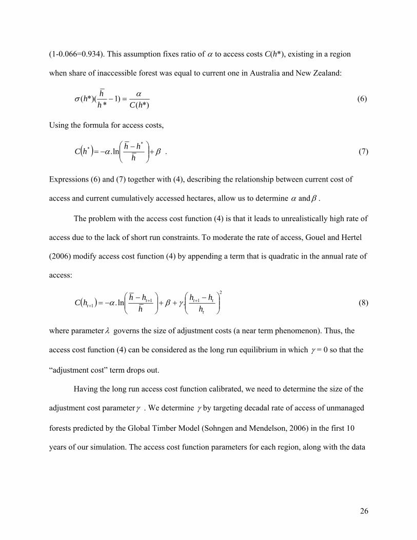
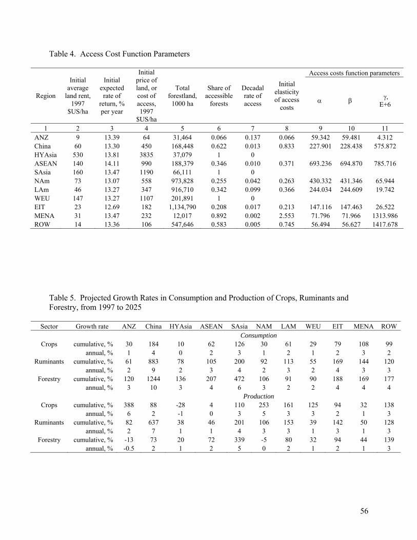
Following Gouel and Hertel (2006), we parameterize the access cost function in each

region by assuming that the elasticity of access costs with respect to cumulative accessed

hectares in Australia and New Zealand – the region with the lowest share of accessible forests

(Table 4) – is equal to the share of accessible forests, that is σ(h) = 0.066. Then, each region’s

α is calibrated such that it would have a very elastic supply of land –very low sensitivity of

access costs with respect to cumulatively accessed forestland – if they were to have the same

inaccessible share of forest land as recently observed in Australia and New Zealand

26

(1-0.066=0.934). This assumption fixes ratio of α to access costs C(h*), existing in a region

when share of inaccessible forest was equal to current one in Australia and New Zealand:

*)()1

**)((

hChhh ασ =− (6)

Using the formula for access costs,

( ) βα +⎟⎟⎠

⎞⎜⎜⎝

⎛ −−=

hhhhC

** ln. . (7)

Expressions (6) and (7) together with (4), describing the relationship between current cost of

access and current cumulatively accessed hectares, allow us to determine α andβ .

The problem with the access cost function (4) is that it leads to unrealistically high rate of

access due to the lack of short run constraints. To moderate the rate of access, Gouel and Hertel

(2006) modify access cost function (4) by appending a term that is quadratic in the annual rate of

access:

( )2

111 .ln. ⎟⎟

⎠

⎞⎜⎜⎝

⎛ −++⎟⎟

⎠

⎞⎜⎜⎝

⎛ −−= ++

+t

tttt h

hhhhhhC γβα (8)

where parameterλ governs the size of adjustment costs (a near term phenomenon). Thus, the

access cost function (4) can be considered as the long run equilibrium in which γ = 0 so that the

“adjustment cost” term drops out.

Having the long run access cost function calibrated, we need to determine the size of the

adjustment cost parameterγ . We determine γ by targeting decadal rate of access of unmanaged

forests predicted by the Global Timber Model (Sohngen and Mendelson, 2006) in the first 10

years of our simulation. The access cost function parameters for each region, along with the data

27

required to determine them, are reported in Table 4. The calibratedγ s are very large, thereby

ensuring that in model simulations the rates of access are quite stable.

The access cost functions are specified at the regional level, thereby augmenting regional

AEZs proportionally, where the proportionate additions are based on the AEZ’s current share of

accessible forests in the total regional accessible forests. The SAGE land cover data, consistent

with GTAP data base definitions of regions and production activities (Lee et al., 2005), is used to

determine land endowments and calculate initial period costs of accessing unmanaged land. We

refer to the Global Timber Model (Sohngen and Mendelson, 2006) to determine the regions

without inaccessible forest land. In Table 4, regions with no inaccessible forests remaining are

High Income Asia, South Asia and Western European Union.

4. Analysis

In this section we first present baseline projections of land use changes from 1997 to 2025 and

then compare results from the sequence of models of land supply. Our baseline model is the most

complex one, including the nested structure of land supply, the soft link with Global Timber

Model to determine the time path of forestry prices, and access to new lands through the

conversion of unmanaged land to land used in production. All other models discussed here may

be viewed as special cases of this baseline model. And by comparing them to the baseline, we

are able to gain insight into the limitations of approaches that omit one or more of the baseline

model features.

28

Baseline

We start from the consumer demand side of the model, as this is the main driver of the demand

for land. Behavior of the AIDADS budget shares, projected with the GE model, is very similar to

that observed in Table 1. However, now, with prices endogenous, consumption depends on

substitution as well as income effects. Table 5 reports the changes in consumer demand for the

land-using sectors. As population and income rise, consumer demands for crops, livestock and

forestry products rise in all regions, with the strongest increases in China, followed by South

Asia (Table 5). Considering three sectors at global scale, the strongest growth in demand is

predicted for forestry products, which reflects rising demands for furniture, construction and

paper products.

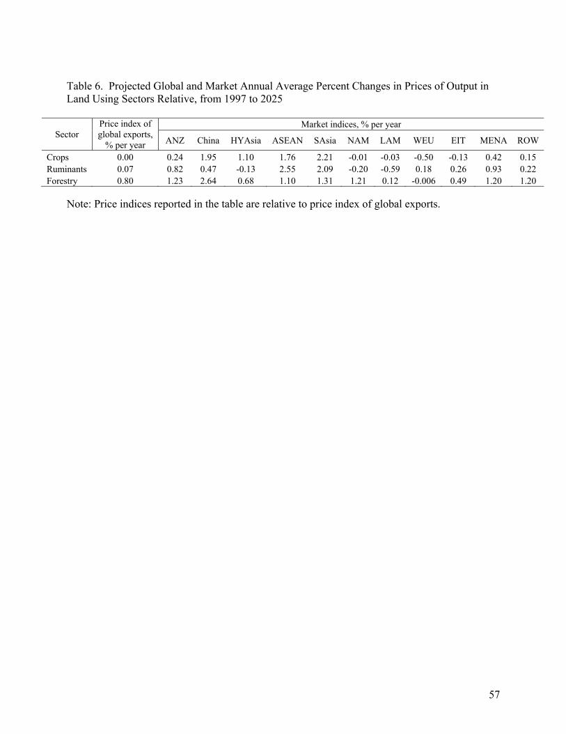
Consumer demand and growth in sectoral productivity, as well as availability of land,

determine prices of output in the land using sectors. The changes in market and global price

indices of output, relative to the price index of world trade, are shown in Table 6. The global

price index for crops is flat over the projections period16 while the global price index of

ruminants increases by a very modest amount (Table 6). The global forestry price is determined

through iteration with Global Timber Model (see discussion above) and increases at 0.8% per

year. This modest, positive rate of growth is consistent with what had been observed historically

(Sohngen et al., this volume). To target this slow rate of price increase, the forestry input-

augmenting technical change is introduced. In our baseline simulation, the forestry input

processing technology is improved at annual rate of 4.2%. This is quite a high rate of technical

progress and will require continued strong innovation in the forest products using sectors.

16 This follows by assumption (see earlier footnote). However, it is nearly true in our model, even without this calibration of global agricultural TFP growth.

29

Prices for forestry output rise in all regions, except Western European Union, where

prices decline very slightly due to relatively strong TFP growth coupled with slow overall

economic growth (Table 6). The growth rate for the crops composite varies considerably by

region. In regions with slow-growing demand and relatively rapid TFP growth in crops (as in the

Americas and Europe), crops prices fall over the baseline. On the other hand, in regions with

high demand growth (China and South Asia) or low (even negative) TFP growth (ASEAN and

High Income Asia), the composite crop price is rising. Prices for ruminants rise in all regions

except for High Income Asia, North America and Latin America, where growth in consumer

demand is weak relative to productivity improvements.

Stronger consumer demand for crops, ruminants and forestry translates into increased

demand for land. Note that in the baseline the land endowment is not fixed, but rather rises in

regions where unmanaged land is available and can be brought into production when land prices

are high. When calibrating the adjustment cost parameters associated with the access cost

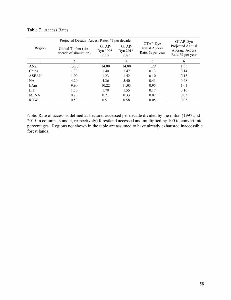
function for unmanaged forests, we target decadal rate of access predicted with the Global

Timber Model. The rate of access is defined as hectares accessed per decade divided by the

initial forestland accessed. These rates, as well as decadal and annual average rates of access

obtained in simulation with GTAP-Dyn, are shown in Table 7. For the first decade of the

simulation, the rates in GTAP-Dyn are similar to ones in the Global Timber Model (due to our

calibration approach). Thereafter, access rates rise a bit due to the increased demand for land, as

well as declining opportunity costs of accessing new land since the rate of return to capital falls

in later periods in all regions, except Economies in Transition.17 The highest rate of access for

17 Rates of access predicted with the Global Timber Model are very stable as well. In the forward model, rates of access tend to decline as prices stabilize over long time horizon.

30

new lands is in Australia and New Zealand, where the share of accessible forests is very low and

accessing new lands is cheap (Table 4); this is followed by Latin and North America.18

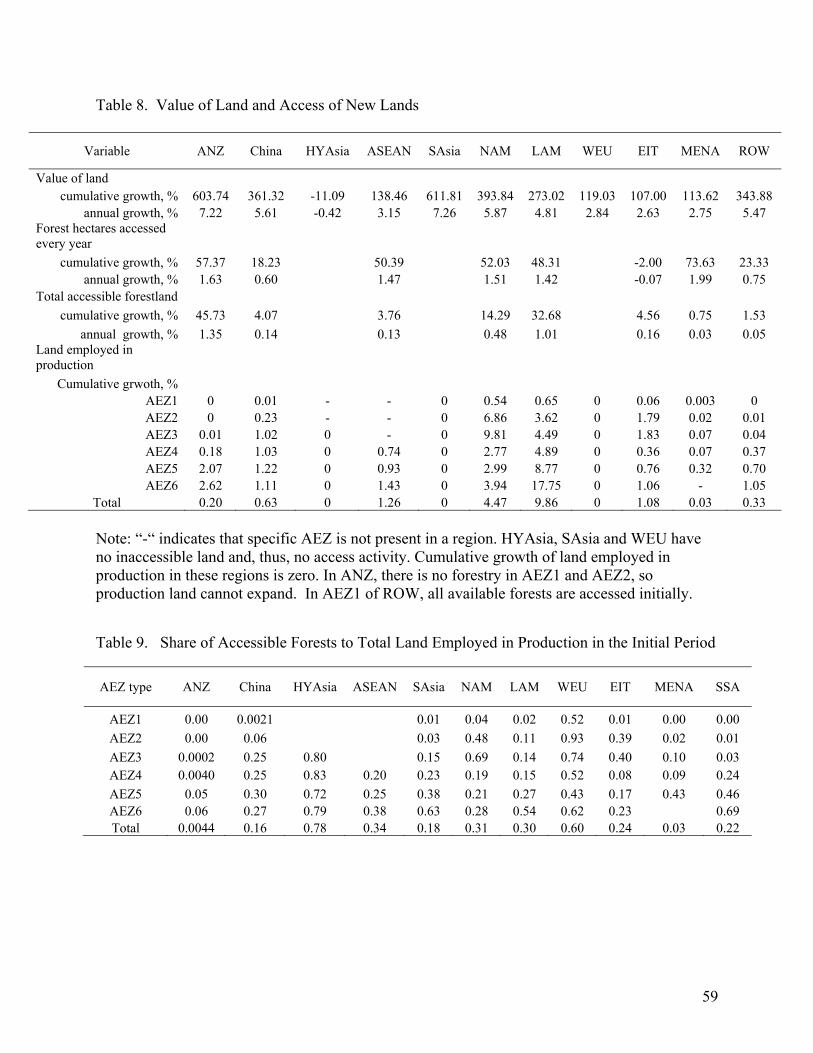
Access to new lands for use in agriculture and forestry is driven by rising land prices in

those sectors, which are themselves a function of the land rental rates in the land-using sectors

and the discount rate. Cumulative and annual growth rates in land values are presented in Table

8. Projected growth in land valuation is highest in South Asia, where consumer demand is strong,

and the aggregate land endowment is fixed. In High Income Asia, the value of land used in

agriculture and forestry (not urban land) is declining, signaling a strong incentive to convert

these lands to other uses (although we do not model this possibility). This declining value of land

is explained by negative TFP growth in crops and forestry, and relatively low TFP growth rate in

ruminants (Table 2), combined with weak consumer demand. Among regions where access to

new lands takes place, the rise in the value of land is highest in Australia and New Zealand,

followed by North America and China.

Table 8 also reports changes in the rate of access to non-commercial, forested lands. This

access rate rises in all regions where such lands are available, except for EIT. The largest growth

in the access rate is 74%, in Middle East and North Africa. This sounds like a large number, until

we recognize that the initial rate of access is very low (just 0.02%: Table 7, column 5)19. As a

result, over the entire period from 1997 to 2025, total accessed forestland expands only to 0.75%

in the MENA region (Table 8, total accessible forest land, cumulative growth rate). In contrast,

from 1997 to 2025, total accessed forestland in Australia and New Zealand expands by 46%.

With relatively moderate growth in forest hectares accessed per year (57%), the 46% expansion 18 As discussed before, we assume that no unmanaged forests are left in High Income Asia, South Asia and Western European Union. 19 The initial annual rate of access is defined as hectares accessed over initial year divided by the initial total accessible forestland.

31

of accessed forests is explained by a very high initial access rate (1% in Australia and New

Zealand, see Table 7). Among regions where access takes place, the growth in value of land is

the slowest in Economies in Transition. The slow growth in value of land is explained by

relatively slow growth in land rents and, unlike other regions in the model, increasing expected

returns to capital. This together with rising wage rates for capital and labor, the two inputs

required to access new lands in the region, results in a decline in hectares accessed per year

(-2%). The initial annual access rate in Economies in Transition is moderate 0.2% (Table 7).

Together with declining hectares accessed per year, total accessed forestland expands by 4.6%

over the projections period (Table 8).

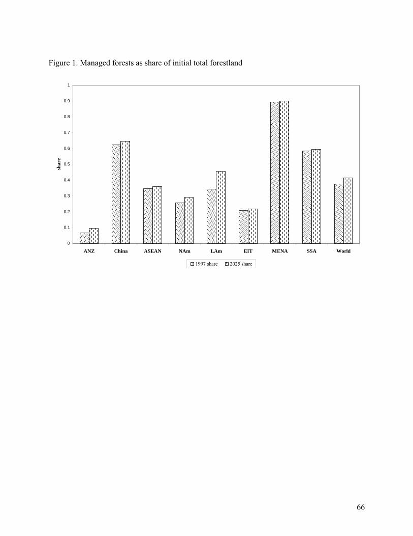
Figure 1 summarizes access activity measured by the share of accessible forests in total

forestland in the initial period (1997). It shows that in Middle East and North Africa very little

unmanaged forests are left in the beginning, and accessed forests expand only marginally. On the

other hand, there is a large scope for expansion in Australia and New Zealand and the Economies

in Transition. From 1997 to 2025, the shares of accessible forests in total forestland increase by

the largest amount in Latin America, followed by Australia and New Zealand and North

America. In Economies in Transition, expansion of accessed forests is tiny because of slow

increase in land value and rising prices of production factors required to access new lands.

Newly accessed land augments the total endowment of land employed in production in

each AEZ (in proportion to the AEZ’s share of accessible forests in the total regional accessible

forests), but only in AEZs where unmanaged forestland is present. Cumulative increase in

production land by AEZ and total for each region are shown in the lower part of Table 8. Thus,

the bottom panel of Table 8 shows that total land employed in production expands in Australia

and New Zealand, but only in AEZ3-AEZ6. In AEZ1 and AEZ2, production land cannot expand

32

because of absence of forestry. Total land in production expands the most in Latin America,

followed by North America. In Australia and New Zealand, growth in accessed forestland is

large (45%), however land employed in production expands only by 0.2% due to the relatively

small share of accessible forests in total land employed in the region (Table 9). In contrast, in

Latin America a relatively large increase in total accessible forests (33%), in fact, translates into

large increase in land employed in production (10%) because initial share of accessible forests in

total production land is high (0.3 in Table 9).

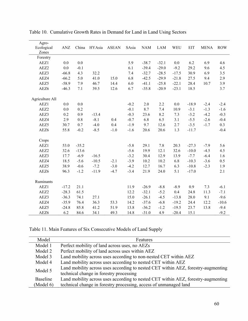
Projected cumulative changes in the demand for land in different sectors and regions are

presented in Table 10. These changes are a result of the redistribution of land across sectors as

well as the enlarged land endowment. In Australia and New Zealand, North America, Latin

America and Western Europe − exporters of agricultural products − land used in commercial

forestry production declines, while agricultural lands expand. Within agriculture, cropland

expands and land in grazing contracts, except for AEZ6 of Australia and New Zealand and Latin

America, where relatively large increases in AEZ land in production is observed (Table 8) and

both, crop and grazing, lands expand over the projections period. In the Economies in Transition,

Middle East and North Africa, South Asia and High Income Asia, land in forestry expands and

agricultural land declines, and, within agriculture, land moves to the ruminants sector.

In ASEAN with only AEZ3 – AEZ6 available, land within agriculture moves to the

ruminants sector. Both forestry and agricultural lands expand in AEZ4 and AEZ5 (recall

unmanaged land can be converted to either of these activities). In AEZ6 of ASEAN, where

forestry is economically quite important (Table 3), forestry expands while land used in

agriculture declines. In China, land in forestry expands in all AEZs except AEZ2 where grazing

land is relatively more important and strong returns to ruminant production result in agriculture

33

bidding land away from forestry. In Rest of the World, forestry expands and agricultural land

declines in all AEZs except the largest AEZ5 dominated by agriculture, where both forestry and

agricultural lands expand. Overall, the baseline results suggest a strong move towards increased

commercial forestry activity in response to increased demand for forest products worldwide in

developing regions, including ASEAN, South Asia and the Rest of the World – three regions

which have experienced extensive deforestation in the past few decades.

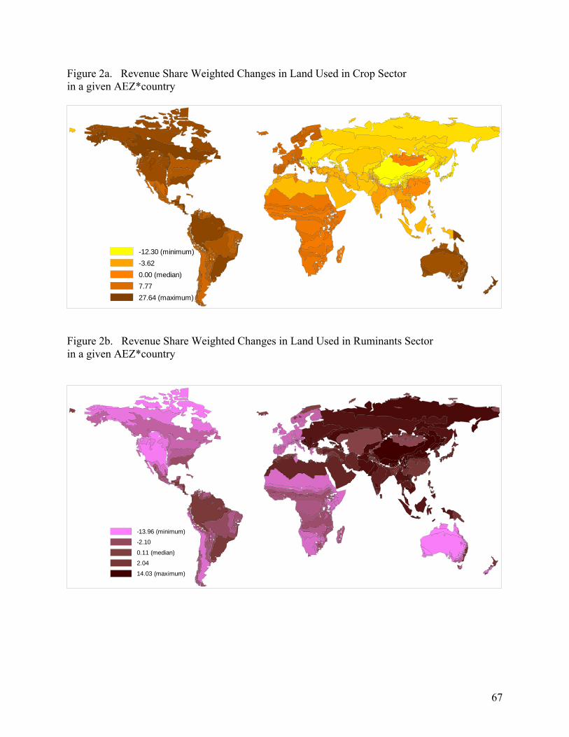
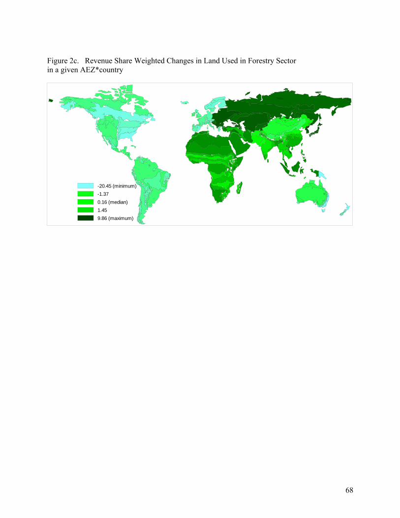
Figures 2a-2c show global maps of revenue share-weighted changes in land use in crops,

ruminants and forestry respectively. The revenue share-weighted changes allow us to evaluate,

and compare across regions, the economic importance of land use changes. Expansion of

cropland is most important in Australia and New Zealand, followed by Americas and Europe,

while the percentage growth in grazing land is largest in China – a region where this represents

overall a relatively smaller claim on land in the base period. Expansion of grazing land is also

important in Economies in Transition, South Asia, ASEAN, and Middle East and North Africa.

Expansion of commercial forestland is important in Economies in Transition, High Income Asia,

ASEAN and Middle East and North Africa.

Determining the Relative Importance of Alternative Supply-side Specifications

Having the main features of the baseline in hand, we now explore the implications of alternative

assumptions made with respect to the specification of land supply. Following discussion in

section 4 of this chapter, we start from a very simple model where land is homogenous and

perfectly mobile across uses, and then successively restrict mobility of land. Throughout this

exercise, we will focus our attention on the implications for land use and land prices.

34

The features of the six models are summarized in Table 11. We start from the simplest

possible model 1, where land is perfectly mobile, and then gradually introduce features to limit

mobility of land across uses. Based on the results obtained with the most highly structured land

supply (model 4), the model is then linked to Global Timber Model to improve forestry

representation (model 5). In model 6, the possibility of conversion of unmanaged forests to land

used in production is introduced. Model 6, our baseline model, includes a nested structure of land

supply, a link with Global Timber Model through the time path of forestry output prices, and the

possibility of conversion of unmanaged land to land used in production. Results of models 1-5

are compared to this baseline model (model 6). To facilitate comparison, productivity growth in

the land using sectors is held constant across six models and fixed at the levels of the baseline

model 6 (recall Table 2). The productivity growth in forestry processing in model 5 is also fixed

at the levels of model 6 to evaluate effect of the introduction of the possibility of conversion of

unmanaged land to land used in production.

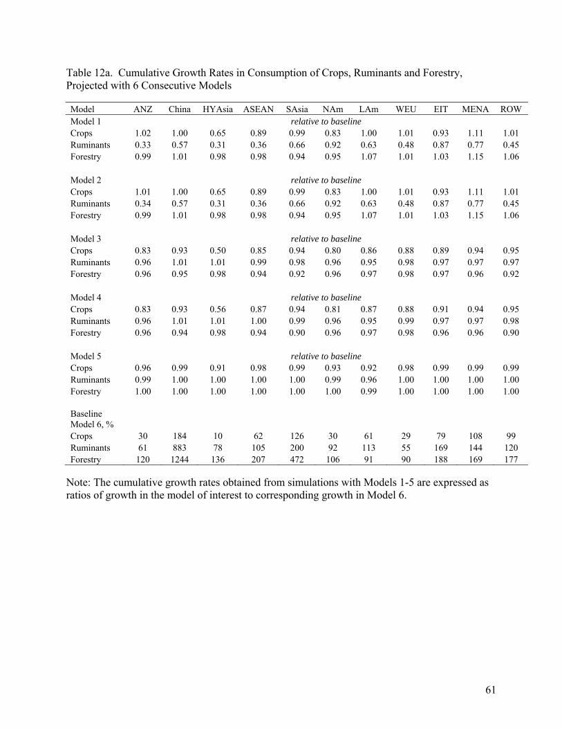
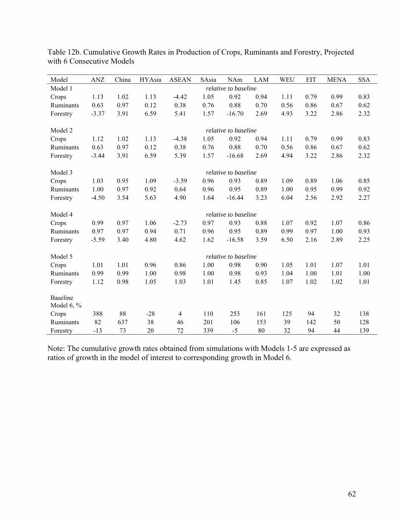
Projected changes in total consumption and production of crops, ruminants and forestry

in all regions are presented in Tables 12a and 12b, respectively.20 Here, the cumulative growth

rates obtained from simulations with Models 1-5 are expressed as ratios of growth in the model

of interest to corresponding growth in model 6. For example, Table 12a shows that ratio of

cumulative growth in consumption of ruminants in ANZ predicted with model 1 is only one third

(0.33) of cumulative growth predicted with the baseline model 6. In Table 12b, cumulative

growth in production of forestry in NAM predicted with model 1 is not only more than 16 times

20 Note, because 17 produced goods are aggregated to 10 consumption goods, direct correspondence between Tables 12a and 12b could be established only for “crops” (see Table 2b). Produced good “ruminants” is part of the consumed aggregate good “MeatDairy”, and produced good “forestry” is part of the consumed aggregate good “Mnfcs” (manufactured goods). Thus, consumer demands for ruminants and forestry are driven by the demands for meat/dairy and manufactured goods, respectively.

35

larger by absolute magnitude than the one predicted by the baseline model 6, but also has

opposite sign. In the baseline production of forestry declines due to the strong forest

input-augmenting technical change. However, this feature is not present in model 1, which

predicts a large expansion of forestry output in NAM and all other regions, relative to baseline.

When presenting the results for land use change, we concentrate our attention on China,

South Asia and Western Europe. These three regions are characterized by very different patterns

of economic growth and land endowments. Economic growth is rapid in China and South Asia,

but slow in Western Europe. However, 38% of forest land in China is unmanaged forests, while

there is none available for conversion in South Asia and Western Europe.

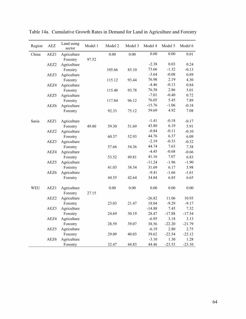
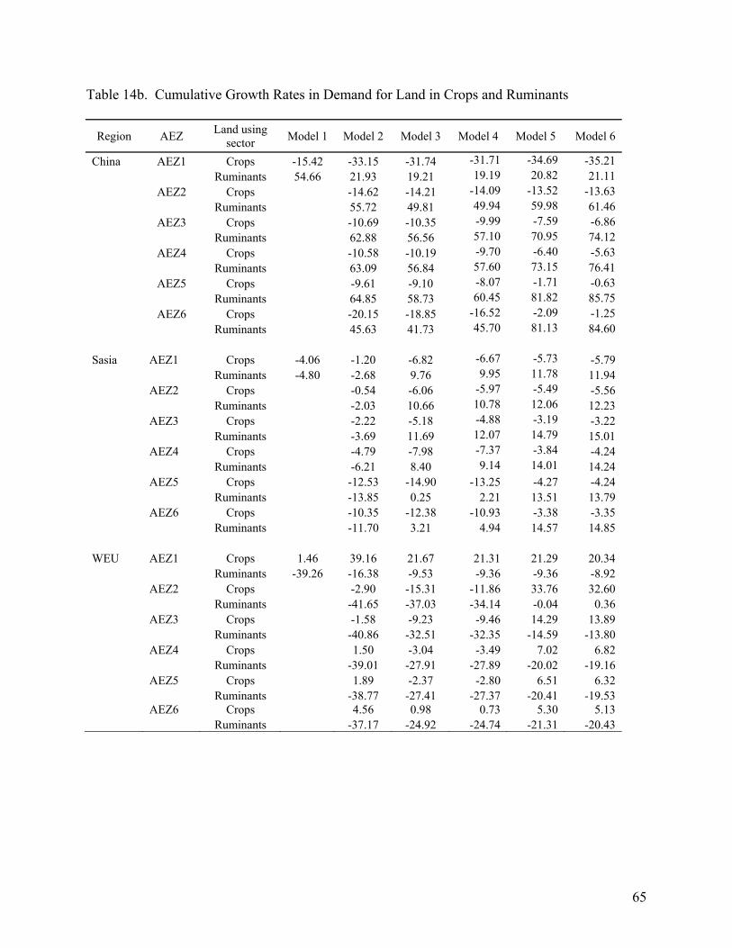
Projected changes in demand for land in land using sectors in the three regions are

presented in Tables 14a and 14b. With the nested CET structure, the land owner first allocates

land between agriculture and forestry, and then between crops and ruminants. When presenting

projected changes in land use, we follow this structure. Table 14a shows distribution of land

between agriculture and forestry and Table 14b shows changes within agriculture. When land is

treated as perfectly mobile across uses (model 1 and model 2) or mobility is restricted by the

non-nested CET (model 3), the decisions about allocation of land among three sectors is taken

simultaneously − nothing is reported for agriculture in Table 14a. When land is considered as a

homogenous endowment (model 1), only one AEZ-generic growth rate appears in the tables.

Now return to tables 12a and 12b. Consumption and production projected with model 1

and model 2 are almost identical. Thus, the introduction of AEZs does not make any difference

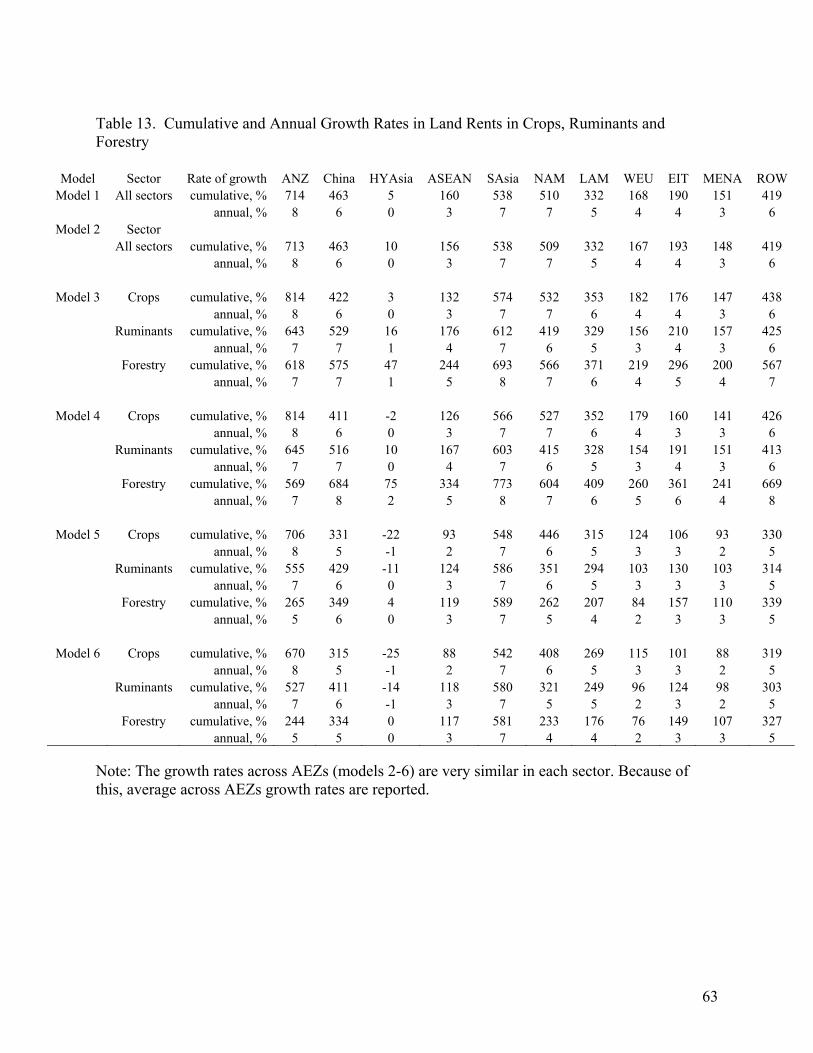
for these aggregate outcomes. With perfect mobility of land across uses, land rents in different

sectors are always equated within AEZ. In light of the fact that different AEZs substitute readily

in a national production function, the land rents across AEZs, but within a given use, will also

36

move together. Thus, in model 2 land rents move together across sectors and AEZs, as in model

1 (Table 13).

Projected changes in land use are also similar across models 1 and 2 (Tables 14a and

14b). With land perfectly mobile across uses (and total land employed in production fixed), in

China, South Asia and Western Europe land moves to that sector with the most rapidly growing

consumer demand −forestry. In South Asia, forest land increases in expense of crops and

ruminants sectors. In China, where rates of growth in demand for forestry and ruminants are

much higher than for crops and TFP growth is much stronger in ruminants then in crops, land

moves from crops to forestry, and also to ruminant production. In Western Europe, where

consumption patterns are very stable and TFP growth in ruminants is much slower than in crops,

land in the ruminant sectors contracts and moves to forestry and crops.

When comparing land use projected with models 1 and 2, note that the economic

importance of a sector in a specific AEZ determines whether magnitude of change predicted with

model 2 is larger or smaller than the one predicted with model 1. Thus, the forestry sector is very

small in AEZs 1-4 in South Asia (Table 3) and therefore has great potential to expand without

excessively bidding up land rents in that AEZ. In fact, projected changes of land use in forestry

in these AEZs are larger than in model 1. In AEZs 5 and 6, where forestry is relatively important,

expansion of forest land bids up land rents very quickly and is therefore smaller than in model 1.

Model 3 introduces restrictions on the mobility of land across uses within a given AEZ

through a CET function. This gives rise to substantial changes in supply, and hence in relative

prices and, therefore consumption. This phenomenon is most striking in the case of ruminants

production. Whereas previously there was a strong tendency (outside of China) to shift land out

of grazing and into crops and/or forestry production, this kind of reallocation is no longer so easy

37

in the presence of finite acreage response elasticities. With more land being retained in ruminant

production, yet the same rate of technical change, prices are accordingly lower and consumption

is higher. On the other hand, consumption of crops and forest products is lower. Note also that

intermediate use and international trade smooth out the production differences resulting in

relatively more uniform changes in consumption across regions (Table 12a). In fact, ruminant

consumption is nearly identical to baseline from model 3 onwards, indicating that the CET

specification is a key feature of the full baseline model.

With the CET in place, the allocation of land across uses is much less responsive to

changes in relative returns to land in different activities and, thus, land rental differentials across

sectors persist. Table 13 shows that, with exception of Australia and New Zealand, introduction

of CET leads to higher land rents in forestry (comparing models 2 and 3), because growth in

demand for forestry is the strongest among three land using sectors worldwide. In China and

South Asia, growth in TFP and consumer demand translates into stronger growth in land rents in

ruminants sector compared to crops. In China, increase in land rents in crops, predicted with

model 3, is even smaller than the one predicted with models 1 and 2. In contrast, in Western

Europe where TFP growth in crops is higher than in the ruminants sectors, land rents in crops

rise stronger than in ruminants.

With restricted mobility of land across uses, projected changes in land use in China are

smaller with model 3 (Table 14a and 14b), however direction of changes is very similar to ones

projected with model 2. Forestland and grazing land expands in all AEZs and crop land

contracts, but the magnitude of changes is smaller than with model 2. As with models 1 and 2,

forest land expands in South Asia. In contrast to models 1 and 2, however, grazing land expands.

Both, forestry and grazing land expand at the expense of cropland, which contracts much faster

38

in each AEZ compared to model 2. Similar to model 2, grazing land declines in Western Europe

in all AEZs, with changes being smaller than in model 2. Crop land, however, also contracts in

AEZs 4 and 5 giving more scope for expansion of land in the forestry sector.

In model 4, the nested CET structure is introduced, whereby the land owner first allocates

land between agriculture and forestry, and then between crops and grazing. This modification

has very little effect on production patterns (Table 12b), and no effect on consumption. Changes

in land use are similar to ones projected with model 3, but in most cases smaller because of more

limited mobility of land between agriculture and forestry (Tables 14a and b). And this more

limited mobility further increases divergence of land rents across uses (Table 13).

Does this divergence in land rents make sense? Are the projected rates of growth in

overall land rents plausible? By way of comparison, it is useful to consider growth in land rents

over the past 100 years in the US. In 1900, the average value of agricultural land and buildings

was just $20 per acre. By 2000, this had risen to $1,050 in constant dollars –an increase of 52

times or 4% per year (NASS, USDA, 2007). Contrast this with the projected annual growth rate

in land rents of 6.78% and 6.03% in crops and livestock, respectively, in North America for

1997-2025 period. The projected rates seem high, especially if we take into account that North

America grows slowly over the projection period.

In light of this concern for excessive growth in land rents, we turn to two additional

aspects of the long run modeling of land use that we believe are required in order to obtain

realistic projections. The first of these has to do with technical change in the forestry using

sectors. In models 1-4, we model technical change in forestry processing sector as labor

augmenting – as with all the non-land using sectors. This ignores the strong technological

improvement in forestry processing sectors observed in the past (recall the discussion of this

39

point in section 2 of this chapter). In model 5, we introduce such forestry input-augmenting

technical change in forestry processing, allowing it to adjust endogenously in order to let the

model track the price path suggested by the Global Timber Model. Comparison of the production

patterns in models 4 and 5 shows huge drop in output of forestry sector (logs) after introduction

of the forest product-augmenting technical change (Table 12b). Fewer logs are needed to

produce the final goods demanded by consumers. At the same time, with lower prices for the

final goods, consumption of these goods increases. The technical change also frees some of the

forest land that now may be used to produce more ruminants and crops. As land becomes less

“scarce”, output prices in the land using sectors decline, leading to larger consumed quantities of

crops and ruminants, as well, in most of the regions (Table 12a).

Forestry input-augmenting technical change reduces pressure on land rents in forestry, as

well as in the other land using sectors. Land rents, projected with model 5, are much smaller,

especially in forestry. They are also less divergent across uses in all regions except Australia and

New Zealand where forestry output projected with model 5 drops below baseline (Table 12b).

Introduction of forestry input-augmenting technical change in forestry processing

significantly affects projected land use changes (Table 14a). In China and South Asia, forestland

grows only by very small amount in most AEZs, or even contracts slightly in AEZ2 of China,

where strong growth in ruminant land demand outbids forestry. Within agriculture, land

continues to expand in the ruminants sector, where returns to land are higher (Table 13), at the

expense of crop land. In Western Europe’s agricultural sectors, crops outbid the other uses of

land and forestry land contracts in all AEZs.

While land rents grow more slowly in model 5 than in previous models, they still grow at

a real rate of 7 or 8 percent per year in some regions. This raises the question of whether

40

previously inaccessible land might be accessed to reduce growth in land rents. Certainly the

investment theory laid out above would suggest that this kind of a rise in land rents would

encourage individuals to invest in roads, infrastructure and deforestation in order to expand the

commercial land base. And access to new land is indeed part of the baseline model (6) from

which results are reported in Tables 12 – 14. Recall that we calibrate the access cost functions to

be initially relatively elastic in those regions with lots of inaccessible land, and inelastic in those

regions on the verge of exhausting their inaccessible land (Table 4, column 8). Also, we set the

adjustment cost parameters in order to broadly replicate the same rate of access in the first

decade as that predicted by the Global Timber Model. As a result, the adjustment cost terms are

quite high and access rates are relatively stable. As a consequence, moving from model 5 to

model 6 will only make a large difference if: a) the access rate in a region is high initially and b)

the initial accessed forest area is large, relative to total land in production, in the same region.

These two conditions hold only in Latin America and North America. In Australia and New

Zealand access rates are high, however initial accessible forest area is tiny comparing to total

production land. Thus, introduction of this last feature changes projections of land use and land

rents only slightly.

Projections obtained with model 6 suggest slightly higher consumer demand for crops in

all regions. Compared to model 5, this is achieved mostly through expansion of output in Latin

and North America, where new access takes place, and reduction of output in Western Europe

(Table 12b). Growth rates in land rents are further reduced in all sectors and regions (Table 13).

In China, expansion of land used in production changes land use patterns. When more land is

available, forest land expands in all AEZs, except AEZ2. Within agriculture, land continues to be

shifted into higher returns ruminant production, at the margin. However, the decline in cropland

41

is smaller than predicted with model 5. In South Asia and Western Europe, where no unmanaged

forests are available, the pattern of land use change is very similar to one predicted with model 5.

The expansion of production land in all other regions smoothes changes in land use in South

Asia and Europe. In South Asia, with highest returns to land in forestry, forestland grows and

agricultural land declines, as in model 5, but at slower rate. In Western Europe, where returns to

agricultural land rise faster than to forestland, agricultural, more specifically cropland, expands

in expense of forests.

5. Summary and Evaluation

An important component of global GHG emissions is related to land use. Yet our ability to

predict long run changes in global land use remains limited. In this chapter we develop a model

designed explicitly to project patterns of land-use change at the global scale over the long run

based on fundamental supply/demand drivers. We start from a dynamic GE model that predicts

economic growth in each region of the world, conditionally on a scenario of productivity

changes, and modify it in order to capture the most important determinants of supply and

demand for land. Because forestry plays an important role in the competition for land and future

path of land-use related GHG emissions, and because a recursive GE model is unable to capture

forestry dynamics, we also link the GE model with forward-looking Global Timber Model in

order to establish a future price path for forest products.

The most important driver of the demand for land is consumer demand, which we model

with econometrically estimated, international cross-section, AIDADS demand system. This

demand system is very flexible in representing changes in the consumption bundle as incomes

rise, which is particularly important in the fast-growing developing countries. The specification

42

of consumer demand influences the scale and location of each land-using production activity

and, hence, associated GHG emission levels. We then introduce recent empirical estimates and

forecasts of technological change in the agricultural sectors to account for the influence of

technology on the demand for land. Technical change in forestry processing sectors is another

key factor in determining demand for land used in forestry sector and outcomes of the

competition for land between forestry and agriculture, and this is determined through the soft

link with the Global Timber Model.

Input substitution is also important in determining sectoral demand for land, which we

incorporate through possibility of intensification in crops, livestock, forestry and food processing

sectors. We allow substitution between land and fertilizers in crops, and substitution amongst

feedstuffs, and between feedstuffs and land, in livestock production, in order to reflect the

empirical evidence that agricultural production tends to intensify in the face of rising land rents.

In forestry, we permit substitution between land and other value added inputs to reflect

sensitivity of output per unit of land with respect to changes in management intensity, predicted

by the Global Timber Model. In food processing, we introduce substitution between farm-based

products and marketing inputs. These intensification possibilities reduce pressure of the growing

consumer demands on land.

Consumer demand is translated into the derived demands for land through a set of

production functions. Equilibrium land rents are determined by equating these demands to land

supply, and we focus considerable attention on how the latter should be modeled, through a

sequence of successively more sophisticated models of land supply. We begin from very simple

model where land endowment is fixed, homogenous and perfectly mobile, and end with one (our

baseline model) which realizes that land endowments are heterogeneous, can be expanded by

43

converting unmanaged land into production land, and where mobility of land across uses is

restricted by a nested CET function within each land type.

In the baseline model, as population and per capita income grow and consumption patters

change, the strongest growth in consumer demand for land-based products is predicted in rapidly

growing China and South Asia. Comparing three land-using sectors globally, the strongest

growth in consumer demand is predicted for forestry, fueled by increasing demand for furniture,

housing and paper products. Increasing consumer demand for crops, livestock and forestry

products translates into increased demand for land, which is reflected in land values. When land

values are high enough to justify investment in the access to new lands, unmanaged forestland

can be converted to production land. Thus, in the baseline, the land endowment is not fixed and

expands in regions where unmanaged forests are available. When introducing the decision to

access unmanaged forests, we draw, again, on the Global Timber Model, by targeting rates of

access of unmanaged forests, predicted by the forestry model. Driven by higher land values,

production land expands in all regions except High Income Asia, South Asia and Western

Europe where no unmanaged forests are available. The largest expansion is projected in Latin

America (9.96%), followed by North America (4.47%), with global production land expanding

by 2.4%.

The redistribution of land across sectors under pressure of changes in relative land rents,

as well as the expansion of land employed in production through new access, combine to result

in land use changes by AEZ. In Australia and New Zealand, North America, Latin America and

Western Europe, land used in forestry production declines and agricultural land expands. Within

agriculture in these regions, more land is used in crop sector and less in livestock production. In

all other regions of the world, including ASEAN, South Asia, and the Rest of the World −three

44

regions which have experienced extensive deforestation in the past − our model predicts

expansion of land employed in commercial forestry and contraction of agricultural land in

response to increased demand for forest-based products worldwide.

Analysis of the sequence of models of land supply reveals that introduction of the

Constant Elasticity of Transformation function to restrict mobility of land across uses within

AEZs is critical for determining relative costs of production in each land using sector, and thus

for consumption and production patterns in all regions of the model. The forestry input-

augmenting technical change is critical in moderating the growth in land demands over the

baseline, thereby freeing land for cropping and grazing activities. In some regions, like Western

Europe, this changes the land use patterns leading to expansion of agricultural land in expense of

forestland. The possibility of accessing new lands further reduces land rents in all land using

sectors and regions, and smoothes changes in land use in the regions where access does not take

place.

It remains to discuss the sensitivity of the baseline to uncertain model parameters, as well

as to evaluate our overall results in light of historical evidence as well as common sense. Since

we build up our estimates of the time path of land rents from fundamental drivers of supply and

demand and not from time trends, perhaps the best overall method of model validation is to

simply look at the rate of growth of land rents in the model. These vary by region, and they only

reflect conditions in agriculture and forestry. So, for example, in High Income Asia, where

consumer demand is weak and TFP rates of growth in these sectors are very slow or negative,

land rents are flat. However, we expect residential, commercial and recreational demands for

land to grow strongly, thereby supporting land rents in agriculture and forestry as well (if only

due to the expectation of profits from future conversion of land to these uses). The growth rates

45

in China’s land rents range from 5 to 6% per year and do not seem out of line with recent

experience in that country. If anything, these may be on the low side. However, once again we

must distinguish between growth in land rents due to agriculture and forestry uses vs. that due to

growth in the demand for land by other sectors which is not treated here.21

Perhaps most surprising is the very strong growth in land rents in the agricultural

exporting regions Australia/New Zealand and North America (4 – 8% per year). Strong TFP

growth – particularly in the crops sectors – supports an expansion of these activities. These

growth rates are generally higher than those observed over the long term in North America (4%

per year over the last century). But there are some reasons to believe that the economic

fundamentals may be in place to support this. In addition to the strong projected TFP growth, and

strong economic growth in the natural resource scarce Asia region, the US (and hence North

America) will have to begin repaying its debts in the future. And our dynamic GE model takes

this into account – showing the region moving into a substantial trade surplus by the end of the

projections period. This bodes well for export-oriented sectors such as agriculture and could

presage a higher rate of growth in agricultural and forestry land rents.

We can also compare projected changes in land use with historical changes.

Unfortunately, we do not presently have data that document changes in land use by AEZ/region.

However, the FAO (FAOSTAT, 2004) provides information on historical changes in land

employed within agriculture. These data suggest that agricultural land in South America

expanded by 14% from 1975 to 2003 (a comparable length of time to our baseline). Our baseline

suggests that this trend will continue with agricultural land expanding from 2.2% in AEZ1 to

21 It is assumed in the model that only crops, ruminant livestock and forestry compete for land, while all other sectors do not use land.

46

20.6% in AEZ6 (Latin America, Table 10). Within agriculture, historical data show that land

expanded much more in cropping activity (22%) than in grazing (12%). Our projections for crop

sector suggest continuing trend with cropland expanded from 7.8% in AEZ1 to 24% in AEZ6

over next 28 years. Projections for livestock depart from the trend suggesting a decline in grazing

land driven by more intensification in livestock production. The changes projected for North

America, however, are very different from the historical trend. FAO reports that from 1975 to

2003 agricultural land use declined, equally in crops and livestock sectors, by 4%, while our

projections suggest large decline in grazing land, but expansion of cropland driven by growth in

exports. Of course, if historical trends were always accurate predictors of the future, there would

be no need for economic models! In light of the recent expansion in crops production in the US,

the recent historical trend in that region may indeed be reversed.

Taking into account the fact that this book focuses heavily on methodology and the

current state of the art in modeling land use in general equilibrium, we close the chapter by

discussing those aspects of this work that we feel most uncomfortable with, and which are in

greatest need of attention in subsequent work. First consider the issue of parametric uncertainty.

While there are many parameters in the model that play a role in determining the long run pattern

of land use, there is one that we single out here for special attention, both because it is important

and we know relatively little about it, and because it is fundamentally amenable to econometric

investigation. This is the elasticity of substitution between feedstuffs and land in the livestock

sector. In our simulations, we assume a value of 0.75 – this is comparable to the elasticities of

substitution amongst feedstuffs in livestock production documented in other studies (Keeney and

Hertel (2005), Peeters and Surry, 1997). Yet we intend for this parameter to capture a broader set

of changes – in particular the scope for intensification of livestock production. Over time, as land

47

rents rise, relative to feed prices, we expect to see more feedlots and a general intensification of

livestock production. This is a key feature of the evolving global livestock industry and it is

important for the determination of land use. For example, when we reduce this possibility by

cutting the elasticity of substitution to 0.2, more land is required to meet the growing consumer

demands for ruminant livestock. In this simulation, grazing land expands in all regions, except

Australia and New Zealand, at the expense of forest land. Forest land expands only in Economies

in Transition and High Income Asia. Thus, our findings about the potential increase in

commercial forests in ASEAN, South Asia and the Rest of the World are very sensitive to the

assumption about intensification in livestock production. On the other hand, setting the elasticity

to substitution to some higher value, would lead to smaller expansion of grazing land in regions

where baseline projects expansion of land employed in livestock (like China), and larger decline

of grazing land in regions where baseline predicts its contraction (like Australia and New

Zealand). Future research efforts should be focused on estimating this parameter using historical

data on the livestock industry.

The second major area of concern relates to the use of Constant Elasticity of

Transformation (CET) functions to restrict land mobility across uses, within AEZs. This is a

popular device in CGE models. It successfully permits these models to be calibrated to estimated

land supply elasticities. However, it prevents us from tracking physical hectares as they move

from one use to another. This is due to the fact that the CET function, true to its name,

transforms hectares in one use to hectares in another use. And these uses have different values.

Higher valued land is deemed more productive. The fundamental constraint in the CET

production possibility frontier for land in a given AEZ is not expressed in terms of individual

hectares, but rather in terms of effective hectares – that is productivity-weighted hectares. Since

48

land is assumed to be paid the value of its marginal product, these are also land rent-weighted

hectares. Thus, the fundamental constraint on the CET function is that the land rental share-

weighted quantities in each use sum to the total change in AEZ hectares available. This is why,

whenever we seek to compare changes in land use, we weight the quantity changes by their value

in use. However, this creates a rift between the physical world and the economic model which

can pose problems when attempting to relate model results back to the physical environment.

Therefore, tractable alternatives to the CET specification would be most desirable.

Finally, we do not believe the present implementation of the land use component of this

model is sufficiently detailed. While the 11 region/6 AEZ/crop-livestock-forestry breakdown

does yield some interesting heterogeneity across AEZs, in future work, we would like to use a

much larger number of AEZs as well as more crops in order to capture the heterogeneity of land

use across AEZs. We believe that the cost of doing so would be relatively small, as long as we

retain the assumption of a single, national production function detailed in this chapter. So, for

example, reducing the Length of Growing Period in each AEZ from 60 to 20 days would seem to

make good sense. This would considerably enrich the physical detail of the ecological constraints

on production in the model at relatively low cost.

49

6. References

Ahammad, H., and R. Mi. “Land Use Change Modeling in GTEM: Accounting for forest sinks”.

Australian Bureau of Agricultural and Resource Economics. Presented at EMF 22:

Climate Change Control Scenarios, Stanford University, California, 25-27 May, 2005.

Choi, S-W., B. Sohngen, and A. Ralph, 2006. “Land Use Change in the Midwestern United

States”, Report prepared for the USDA Forest Service, Pacific Northwest Research Lab,

Corvallis, Oregon.

Cranfield, J.A.L., J.S. Eales, T.W. Hertel, and P.V. Preckel, 2003. “Model Selection when

Estimating and Predicting Consumer Demands using International, Cross Section Data,”

Empirical Economics, 28(2):353-364.

Darwin, R., Tsigas, M., Lewandrowski, J. and Raneses, A., 1995. World Agriculture and

Climate Change: Economic Adaptations, Agricultural Economic Report no. 703,

Economic Research Service, US Department of Agriculture, Washington DC.

Dimaranan, B. V., and R. A. McDougall, 2002. “Global Trade, Assistance, and

Production: The GTAP 5 Data Base,” Center for Global Trade Analysis, Purdue

University, available on line at

http://www.gtap.agecon.purdue.edu/databases/v5/v5_doco.asp.

Economic Research Service, US Department of Agriculture, Briefing Rooms, 2006. “Food

Marketing and Farm Spreads: USDA Marketing Bill”, available on line at

http://www.ers.usda.gov/Briefing/FoodPriceSpreads/bill/table1.htm.

FAOSTAT, 2004.

50

Gale, F., and K. Huang, 2007. “Demand for Food Quantity and Quality in China”, Economic

Research Report No. (ERR-32). Economic Research Service, U.S. Department of

Agriculture, available on line at http://www.ers.usda.gov/publications/err32 .

Global Timber Market and Forestry Data Project, 2004. Available on line at

http://www-agecon.ag.ohio-state.edu/people/sohngen.1/forests/GTM/index.htm

Golub, A. 2006. Projecting the Global Economy to 2025: A Dynamic General Equilibrium

Approach. Ph.D. dissertation, Purdue University.

Golub, A. and R. McDougall, 2006. “New Household Saving Behavior in the Dynamic GTAP

model”. Paper prepared for the presentation at the Ninth Annual Conference on Global

Economic Analysis, Addis Ababa, Ethiopia, June 15 - 17, 2006.

Haynes, R., 2003. An Analysis of the Timber Situation in the United States: 1952-2050. U.S.

Department of Agriculture, Forest Service, Pacific Northwest Research Station, General

Technical Report, PNW-GTR-560. Portland, OR.

Hertel, T.W., ed. 1997. Global Trade Analysis Modeling and Applications. Cambridge

University Press.

Hertel, T.W., H.-L. Lee, S. Rose, B. Sohngen. “The Role of Global Land Use in Determining

Greenhouse Gases Mitigation Costs”. This volume.

Hertel, T. W., C. E. Ludena, and A. Golub, 2006. “Economic Growth, Technological Change

and Patterns of Food and Agricultural trade in Asia”. ERD Working Paper No. 86, Asian

Development Bank, November.

Hertel, T.W. and M. Tsigas, 2002. “Primary Factor Shares”, Global Trade, Assistance, and

Production: The GTAP 5 Data Base, Center for Global Trade Analysis, Purdue

51

University, available on line at

https://www.gtap.agecon.purdue.edu/resources/download/870.pdf.

Ianchovichina, E. and R. McDougall, 2001. Structure of Dynamic GTAP. GTAP Technical Paper

17, Center for Global Trade Analysis, available on line at www.gtap.org.

Keeney, R., and T.W. Hertel, 2005. GTAP-AGR: A Framework for Assessing the Implications of

Multilateral Changes in Agricultural Policies. GTAP Technical Paper 24, Center for

Global Trade Analysis, available on line at www.gtap.org.

Kets, W., and A.M. Lejour, 2003. Sectoral TFP growth in the OECD, CPB Memorandum 58.

Lee, H-L., T. W. Hertel, B. Sohngen and N. Ramankutty, 2005. Towards and Integrated Land

Use Data Base for Assessing the Potential for Greenhouse Gas Mitigation. GTAP

Technical Paper No. 25, Center for Global Trade Analysis, Purdue University, available

on line at

https://www.gtap.agecon.purdue.edu/resources/res_display.asp?RecordID=1900.

Ludena, C., 2005. Productivity Growth in Crops and Livestock and Implications to World Food

Trade. Ph.D. Dissertation, Purdue University, (2005).

National Agricultural Statistical Service, United states Department of Agriculture, 2007. “Trends

in U.S. Agriculture” http://www.usda.gov/nass/pubs/trends/landvalue.htm

Organization for Economic Cooperation and Development. (2001). Market Effects of Crop

Support Measures, OECD Publications, Paris, France.

Peeters, L. and Y. Surry. (1997). “A Review of the Arts of Estimating Price-Responsiveness of

Feed Demand in the European Union,” Journal of Agricultural Economics, 48: 379-392.

52

Reimer, J.J. and T.W. Hertel, 2004. “Estimation of International Demand Behavior for Use with

Input-Output Based Data,” Economic Systems Research, 16(4): 347-366.

Rimmer, M.T., and A.A. Powell, 1996. “An Implicitly Additive Demand System.”

Applied Economics 28:1613-1622.

Ronneberger, K., M. Berrittella, F. Bosello and R.S.J. Tol. “KLUM@GTAP: Spacially-Explicit,

Biophysical Land Use in a Computable Equilibrium Model”. This volume.

Sohngen, B. and R. Mendelsohn, 2006. “A Sensitivity Analysis of Carbon Sequestration”. In

Human-Induced Climate Change: An Interdisciplinary Assessment. Edited by M.

Schlezinger. Cambridge University Press.

Sohngen, B., R. Mendelsohn and R. Sedjo, 1999. “Forest Management, Conservation, and

Global Timber Markets”. American Journal of Agricultural Economics, 81(1):1-13.

Sohngen, B., Tennity, C., Hnytka, M., and K. Meeusen, forthcoming. “Global Forestry Data for

the Economic Modeling of Land Use”. This volume.

US-EPA, Global Emissions of Non-CO2 Greenhouse Gases: 1990-2020, Office of Air and

Radiation, US Environmental Protection Agency (US-EPA), Washington, D.C.,

forthcoming.

Walmsley, T. L., Dimaranan B. V., and R. A. McDougall, 2000. “A Base Case Scenario for the

Dynamic GTAP Model”, Center for Global Trade Analysis, Purdue University.

Wohlgenant, M. K., 1989. “Demand in Farm Output in a Complete System of Demand

Functions”. American Journal of Agricultural Economics, Vol. 71, No. 2, pp. 241-252.

Yu, W., Hertel, T. W., Preckel, P. V., and J. S. Eales, 2002. “Projecting World Food Demand

using Alternative Demand Systems”. Economic Modeling, 21: 99-129.

53

Table 1. Beginning, and projected end-of-period budget shares, assuming constant prices, based on exogenous income and population growth in the baseline

Region Year Growth in per capita income

Crops Meat Dairy

OthFood Bev

Text Appar

HousUtils

WR Trade Mnfcs Trans

Comm Fin

ServiceHous

OthServ

ANZ 1997 0.01 0.03 0.09 0.03 0.04 0.24 0.09 0.09 0.03 0.35 2025 102% 0.01 0.02 0.07 0.03 0.04 0.25 0.08 0.09 0.04 0.38

China 1997 0.20 0.16 0.12 0.09 0.02 0.10 0.14 0.06 0.04 0.08 2025 512% 0.04 0.13 0.06 0.10 0.03 0.15 0.18 0.09 0.09 0.13

HYAsia 1997 0.03 0.02 0.08 0.04 0.05 0.24 0.10 0.10 0.03 0.31 2025 96% 0.01 0.02 0.07 0.03 0.05 0.26 0.09 0.10 0.04 0.34

ASEAN 1997 0.09 0.07 0.12 0.06 0.04 0.12 0.17 0.08 0.06 0.21 2025 126% 0.05 0.06 0.09 0.05 0.04 0.13 0.16 0.08 0.08 0.26

SAsia 1997 0.24 0.12 0.08 0.09 0.02 0.11 0.08 0.12 0.03 0.12 2025 195% 0.11 0.10 0.04 0.10 0.02 0.14 0.10 0.16 0.05 0.18

NAM 1997 0.01 0.02 0.05 0.03 0.05 0.20 0.10 0.07 0.10 0.37 2025 78% 0.00 0.02 0.04 0.03 0.05 0.21 0.09 0.07 0.11 0.39

LAM 1997 0.05 0.08 0.13 0.08 0.05 0.16 0.16 0.12 0.03 0.14 2025 88% 0.03 0.07 0.10 0.08 0.05 0.18 0.15 0.13 0.04 0.17

WEU 1997 0.01 0.05 0.06 0.04 0.05 0.22 0.14 0.10 0.12 0.21 2025 106% 0.01 0.04 0.05 0.04 0.05 0.23 0.13 0.09 0.14 0.23

EIT 1997 0.05 0.13 0.13 0.04 0.08 0.10 0.13 0.10 0.06 0.18 2025 157% 0.03 0.10 0.09 0.04 0.09 0.12 0.13 0.11 0.08 0.23

MENA 1997 0.09 0.08 0.12 0.06 0.04 0.15 0.12 0.11 0.03 0.19 2025 57% 0.06 0.07 0.11 0.05 0.04 0.17 0.12 0.11 0.03 0.23

ROW 1997 0.10 0.09 0.14 0.05 0.03 0.19 0.11 0.10 0.06 0.13 2025 57% 0.07 0.08 0.12 0.05 0.04 0.21 0.11 0.10 0.07 0.15

Note: These calculations assume constant prices and are based on exogenous income and population growth in the baseline. Projections are obtained using GAMS and based on projected income per capital growth calculated using GTAP baseline (Walmsley et al., 2000)

54

Table 2. Annual Average Total Factor Productivity Growth Rates in Agriculture and Forestry Sectors

Region TFP, % per year

Crops Rumin. NonRumin. Forestry ANZ 1.42 0.56 0.92 1.11 China 1.63 3.66 6.70 1.75 HYAsia -0.13 0.56 0.92 -0.05 ASEAN -0.13 -0.83 3.47 -0.18 SAsia 1.13 1.57 3.35 1.23 NAm 1.42 0.56 0.92 1.15 LAm 1.00 1.64 4.94 1.13 WEU 1.42 0.56 0.92 1.10 EIT 1.95 0.65 2.49 1.51 MENA 0.47 -0.11 -0.04 0.31 ROW 1.14 0.80 0.15 1.08

Note: The TFP growth rates are different from the rates reported in Ludena (2005) by common across agricultural sectors and regions adjustment factor. The factor is chosen such that world crop price index moves closely with the price index of traded goods and services. Also, we depart from Ludena (2005) assuming that crops TFP in HYAsia is equal to one in ASEAN, much slower than in the other industrialized regions.

55

Table 3. Land earnings by sector and AEZ for 11 regions of the model

Regions Sectors AEZ1 AEZ2 AEZ3 AEZ4 AEZ5 AEZ6 All Sector ANZ Crops 0.23 0.45 0.66 0.66 0.51 0.20 0.46 Ruminants 0.77 0.55 0.33 0.28 0.08 0.18 0.26 Forestry 0.00 0.00 0.003 0.06 0.41 0.62 0.28 AEZ 0.03 0.13 0.18 0.14 0.24 0.27 1.00 China Crops 0.40 0.81 0.88 0.89 0.92 0.82 0.85 Ruminants 0.60 0.16 0.08 0.07 0.01 0.01 0.04 Forestry 0.00 0.03 0.04 0.04 0.07 0.17 0.11 AEZ 0.01 0.06 0.12 0.11 0.19 0.51 1 HYAsia Crops 0 0 0.68 0.81 0.87 0.78 0.83 Ruminants 0 0 0.05 0.04 0.06 0.06 0.05 Forestry 0 0 0.27 0.15 0.07 0.16 0.12 AEZ 0 0 0.01 0.38 0.47 0.14 1.00 ASEAN Crops 0 0 0 0.94 0.91 0.77 0.82 Ruminants 0 0 0 0.04 0.06 0.05 0.05 Forestry 0 0 0 0.02 0.04 0.17 0.13 AEZ 0 0 0 0.18 0.16 0.67 1.00 SAsia Crops 0.67 0.69 0.81 0.76 0.67 0.73 0.76 Ruminants 0.30 0.30 0.15 0.16 0.10 0.08 0.16 Forestry 0.03 0.02 0.04 0.09 0.24 0.19 0.08 AEZ 0.03 0.12 0.42 0.29 0.11 0.04 1.00 NAM Crops 0.36 0.63 0.50 0.75 0.69 0.51 0.63 Ruminants 0.59 0.30 0.12 0.10 0.08 0.02 0.12 Forestry 0.05 0.07 0.39 0.15 0.23 0.46 0.25 AEZ 0.03 0.10 0.13 0.36 0.15 0.23 1.00 LAM Crops 0.61 0.62 0.62 0.73 0.66 0.74 0.70 Ruminants 0.34 0.26 0.26 0.22 0.22 0.18 0.21 Forestry 0.05 0.12 0.12 0.05 0.12 0.08 0.09 AEZ 0.03 0.06 0.09 0.24 0.22 0.35 1.00 WEU Crops 0.12 0.05 0.25 0.47 0.49 0.56 0.43 Ruminants 0.88 0.32 0.25 0.25 0.25 0.31 0.25 Forestry 0.00 0.64 0.50 0.28 0.26 0.13 0.32 AEZ 0.00 0.03 0.19 0.45 0.29 0.04 1.00 EIT Crops 0.18 0.70 0.76 0.73 0.70 0.51 0.73 Ruminants 0.07 0.16 0.10 0.11 0.18 0.09 0.12 Forestry 0.74 0.14 0.13 0.16 0.12 0.40 0.15 AEZ 0.00 0.17 0.35 0.43 0.05 0.00 1.00 MENA Crops 0.48 0.71 0.54 0.73 0.81 0.00 0.62 Ruminants 0.26 0.18 0.09 0.05 0.03 0.00 0.17 Forestry 0.25 0.11 0.38 0.21 0.16 0.00 0.21 0.27 0.44 0.16 0.13 0.00 0.00 1.00 ROW Crops 0.21 0.35 0.76 0.72 0.75 0.50 0.66 Ruminants 0.46 0.39 0.16 0.06 0.13 0.14 0.12 Forestry 0.34 0.26 0.09 0.22 0.12 0.35 0.22 AEZ 0.01 0.02 0.07 0.27 0.35 0.29 1.00

Note: The land earnings shares are based on GTAP Land Use Data Base, Release 1.0, December 2005, with revised land rents in forestry (see footnote 8 in the text).

56

Table 4. Access Cost Function Parameters

Region

Initial average

land rent, 1997

$US/ha

Initial expected rate of

return, % per year

Initial price of land, or cost of access, 1997

$US/ha

Total forestland,

1000 ha

Share of accessible

forests

Decadal rate of access

Initial elasticity of access

costs

Access costs function parameters

α β γ, E+6

1 2 3 4 5 6 7 8 9 10 11 ANZ 9 13.39 64 31,464 0.066 0.137 0.066 59.342 59.481 4.312 China 60 13.30 450 168,448 0.622 0.013 0.833 227.901 228.438 575.872 HYAsia 530 13.81 3835 37,079 1 0 ASEAN 140 14.11 990 188,379 0.346 0.010 0.371 693.236 694.870 785.716 SAsia 160 13.47 1190 66,111 1 0 NAm 73 13.07 558 973,828 0.255 0.042 0.263 430.332 431.346 65.944 LAm 46 13.27 347 916,710 0.342 0.099 0.366 244.034 244.609 19.742 WEU 147 13.27 1107 201,891 1 0 EIT 23 12.69 182 1,134,790 0.208 0.017 0.213 147.116 147.463 26.522 MENA 31 13.47 232 12,017 0.892 0.002 2.553 71.796 71.966 1313.986 ROW 14 13.36 106 547,646 0.583 0.005 0.745 56.494 56.627 1417.678

Table 5. Projected Growth Rates in Consumption and Production of Crops, Ruminants and Forestry, from 1997 to 2025

Sector Growth rate ANZ China HYAsia ASEAN SAsia NAM LAM WEU EIT MENA ROW Consumption

Crops cumulative, % 30 184 10 62 126 30 61 29 79 108 99 annual, % 1 4 0 2 3 1 2 1 2 3 2

Ruminants cumulative, % 61 883 78 105 200 92 113 55 169 144 120 annual, % 2 9 2 3 4 2 3 2 4 3 3

Forestry cumulative, % 120 1244 136 207 472 106 91 90 188 169 177 annual, % 3 10 3 4 6 3 2 2 4 4 4

Production Crops cumulative, % 388 88 -28 4 110 253 161 125 94 32 138

annual, % 6 2 -1 0 3 5 3 3 2 1 3 Ruminants cumulative, % 82 637 38 46 201 106 153 39 142 50 128

annual, % 2 7 1 1 4 3 3 1 3 1 3 Forestry cumulative, % -13 73 20 72 339 -5 80 32 94 44 139

annual, % -0.5 2 1 2 5 0 2 1 2 1 3

57

Table 6. Projected Global and Market Annual Average Percent Changes in Prices of Output in Land Using Sectors Relative, from 1997 to 2025

Sector Price index of global exports,

% per year

Market indices, % per year

ANZ China HYAsia ASEAN SAsia NAM LAM WEU EIT MENA ROW

Crops 0.00 0.24 1.95 1.10 1.76 2.21 -0.01 -0.03 -0.50 -0.13 0.42 0.15 Ruminants 0.07 0.82 0.47 -0.13 2.55 2.09 -0.20 -0.59 0.18 0.26 0.93 0.22 Forestry 0.80 1.23 2.64 0.68 1.10 1.31 1.21 0.12 -0.006 0.49 1.20 1.20

Note: Price indices reported in the table are relative to price index of global exports.

58

Table 7. Access Rates

Region

Projected Decadal Access Rates, % per decade GTAP-Dyn

Initial Access Rate, % per year

GTAP-Dyn Projected Annual Average Access Rate, % per year

Global Timber (first decade of simulation)

GTAP-Dyn 1998-

2007

GTAP-Dyn 2016-

2025 1 2 3 4 5 6

ANZ 13.70 14.00 14.80 1.29 1.35 China 1.30 1.40 1.47 0.13 0.14 ASEAN 1.00 1.23 1.42 0.10 0.13 NAm 4.20 4.36 5.40 0.41 0.48 LAm 9.90 10.22 11.03 0.95 1.01 EIT 1.70 1.70 1.55 0.17 0.16 MENA 0.20 0.21 0.33 0.02 0.03 ROW 0.50 0.51 0.58 0.05 0.05

Note: Rate of access is defined as hectares accessed per decade divided by the initial (1997 and 2015 in columns 3 and 4, respectively) forestland accessed and multiplied by 100 to convert into percentages. Regions not shown in the table are assumed to have already exhausted inaccessible forest lands.

59

Table 8. Value of Land and Access of New Lands

Variable ANZ China HYAsia ASEAN SAsia NAM LAM WEU EIT MENA ROW

Value of land cumulative growth, % 603.74 361.32 -11.09 138.46 611.81 393.84 273.02 119.03 107.00 113.62 343.88

annual growth, % 7.22 5.61 -0.42 3.15 7.26 5.87 4.81 2.84 2.63 2.75 5.47 Forest hectares accessed every year

cumulative growth, % 57.37 18.23 50.39 52.03 48.31 -2.00 73.63 23.33 annual growth, % 1.63 0.60 1.47 1.51 1.42 -0.07 1.99 0.75

Total accessible forestland cumulative growth, % 45.73 4.07 3.76 14.29 32.68 4.56 0.75 1.53

annual growth, % 1.35 0.14 0.13 0.48 1.01 0.16 0.03 0.05 Land employed in production

Cumulative grwoth, % AEZ1 0 0.01 - - 0 0.54 0.65 0 0.06 0.003 0 AEZ2 0 0.23 - - 0 6.86 3.62 0 1.79 0.02 0.01 AEZ3 0.01 1.02 0 - 0 9.81 4.49 0 1.83 0.07 0.04 AEZ4 0.18 1.03 0 0.74 0 2.77 4.89 0 0.36 0.07 0.37 AEZ5 2.07 1.22 0 0.93 0 2.99 8.77 0 0.76 0.32 0.70 AEZ6 2.62 1.11 0 1.43 0 3.94 17.75 0 1.06 - 1.05

Total 0.20 0.63 0 1.26 0 4.47 9.86 0 1.08 0.03 0.33 Note: “-“ indicates that specific AEZ is not present in a region. HYAsia, SAsia and WEU have no inaccessible land and, thus, no access activity. Cumulative growth of land employed in production in these regions is zero. In ANZ, there is no forestry in AEZ1 and AEZ2, so production land cannot expand. In AEZ1 of ROW, all available forests are accessed initially. Table 9. Share of Accessible Forests to Total Land Employed in Production in the Initial Period

AEZ type ANZ China HYAsia ASEAN SAsia NAM LAM WEU EIT MENA SSA

AEZ1 0.00 0.0021 0.01 0.04 0.02 0.52 0.01 0.00 0.00 AEZ2 0.00 0.06 0.03 0.48 0.11 0.93 0.39 0.02 0.01 AEZ3 0.0002 0.25 0.80 0.15 0.69 0.14 0.74 0.40 0.10 0.03 AEZ4 0.0040 0.25 0.83 0.20 0.23 0.19 0.15 0.52 0.08 0.09 0.24 AEZ5 0.05 0.30 0.72 0.25 0.38 0.21 0.27 0.43 0.17 0.43 0.46 AEZ6 0.06 0.27 0.79 0.38 0.63 0.28 0.54 0.62 0.23 0.69 Total 0.0044 0.16 0.78 0.34 0.18 0.31 0.30 0.60 0.24 0.03 0.22

60

Table 10. Cumulative Growth Rates in Demand for Land in Land Using Sectors

Agro-Ecological

Zones ANZ China HYAsia ASEAN SAsia NAM LAM WEU EIT MENA ROW

Forestry AEZ1 0.0 0.0 5.9 -38.7 -32.1 0.0 6.2 6.9 4.6 AEZ2 0.0 -0.1 6.1 -39.4 -29.0 -9.2 29.2 9.6 4.5 AEZ3 -66.8 4.3 32.2 7.4 -32.7 -28.5 -17.5 30.9 6.9 3.5 AEZ4 -66.2 5.0 41.0 15.0 6.8 -42.5 -29.9 -21.8 27.5 9.4 2.9 AEZ5 -58.9 7.9 46.7 14.4 6.0 -41.1 -25.8 -22.1 28.4 10.7 3.9 AEZ6 -46.3 7.1 39.5 12.6 6.7 -35.8 -20.9 -23.1 18.5 3.7

Agriculture All

AEZ1 0.0 0.0 -0.2 2.0 2.2 0.0 -18.9 -2.4 -2.4 AEZ2 0.0 0.2 -0.1 8.7 7.4 10.9 -3.1 -1.3 -1.6 AEZ3 0.2 0.9 -13.4 -0.3 23.6 8.2 7.3 -3.2 -4.2 -0.3 AEZ4 2.9 0.8 -8.1 0.4 -0.7 6.8 6.5 3.1 -5.5 -2.6 -0.4 AEZ5 30.7 0.7 -4.0 0.4 -1.9 9.7 12.6 2.7 -3.5 -1.7 0.3 AEZ6 55.8 -0.2 -8.5 -1.0 -1.6 20.6 20.6 1.3 -11.7 -0.4

Crops AEZ1 53.0 -35.2 -5.8 29.1 7.8 20.3 -27.3 -7.9 5.6 AEZ2 32.6 -13.6 -5.6 19.9 12.1 32.6 -10.0 -4.5 4.5 AEZ3 17.7 -6.9 -16.5 -3.2 30.4 12.9 13.9 -7.7 -6.4 1.6 AEZ4 18.5 -5.6 -10.5 -2.1 -3.9 10.2 10.2 6.8 -10.3 -3.6 0.5 AEZ5 38.9 -0.6 -7.2 -3.0 -4.2 12.7 16.7 6.3 -10.8 -2.3 1.9 AEZ6 96.3 -1.2 -11.9 -4.7 -3.4 21.9 24.0 5.1 -17.0 2.1

Ruminants

AEZ1 -17.2 21.1 11.9 -26.9 -8.8 -8.9 0.9 7.3 -6.1 AEZ2 -28.3 61.5 12.2 -32.1 -5.2 0.4 24.8 11.3 -7.1 AEZ3 -36.3 74.1 27.1 15.0 -26.1 -4.5 -13.8 28.0 9.1 -9.6 AEZ4 -35.9 76.4 36.3 53.3 14.2 -37.6 -6.8 -19.2 24.4 12.2 -10.6 AEZ5 -24.8 85.8 41.2 51.9 13.8 -36.2 -1.2 -19.5 23.7 13.8 -9.4 AEZ6 6.2 84.6 34.1 49.3 14.8 -31.0 4.9 -20.4 15.1 -9.2

Table 11. Main Features of Six Consecutive Models of Land Supply

Model Features Model 1 Perfect mobility of land across uses, no AEZs Model 2 Perfect mobility of land across uses within AEZ Model 3 Land mobility across uses according to non-nested CET within AEZ Model 4 Land mobility across uses according to nested CET within AEZ

Model 5 Land mobility across uses according to nested CET within AEZ, forestry-augmenting technical change in forestry processing

Baseline (Model 6)

Land mobility across uses according to nested CET within AEZ, forestry-augmenting technical change in forestry processing, access of unmanaged land

61

Table 12a. Cumulative Growth Rates in Consumption of Crops, Ruminants and Forestry, Projected with 6 Consecutive Models Model ANZ China HYAsia ASEAN SAsia NAm LAm WEU EIT MENA ROW Model 1 relative to baseline Crops 1.02 1.00 0.65 0.89 0.99 0.83 1.00 1.01 0.93 1.11 1.01 Ruminants 0.33 0.57 0.31 0.36 0.66 0.92 0.63 0.48 0.87 0.77 0.45 Forestry 0.99 1.01 0.98 0.98 0.94 0.95 1.07 1.01 1.03 1.15 1.06 Model 2 relative to baseline Crops 1.01 1.00 0.65 0.89 0.99 0.83 1.00 1.01 0.93 1.11 1.01 Ruminants 0.34 0.57 0.31 0.36 0.66 0.92 0.63 0.48 0.87 0.77 0.45 Forestry 0.99 1.01 0.98 0.98 0.94 0.95 1.07 1.01 1.03 1.15 1.06 Model 3 relative to baseline Crops 0.83 0.93 0.50 0.85 0.94 0.80 0.86 0.88 0.89 0.94 0.95 Ruminants 0.96 1.01 1.01 0.99 0.98 0.96 0.95 0.98 0.97 0.97 0.97 Forestry 0.96 0.95 0.98 0.94 0.92 0.96 0.97 0.98 0.97 0.96 0.92 Model 4 relative to baseline Crops 0.83 0.93 0.56 0.87 0.94 0.81 0.87 0.88 0.91 0.94 0.95 Ruminants 0.96 1.01 1.01 1.00 0.99 0.96 0.95 0.99 0.97 0.97 0.98 Forestry 0.96 0.94 0.98 0.94 0.90 0.96 0.97 0.98 0.96 0.96 0.90 Model 5 relative to baseline Crops 0.96 0.99 0.91 0.98 0.99 0.93 0.92 0.98 0.99 0.99 0.99 Ruminants 0.99 1.00 1.00 1.00 1.00 0.99 0.96 1.00 1.00 1.00 1.00 Forestry 1.00 1.00 1.00 1.00 1.00 1.00 0.99 1.00 1.00 1.00 1.00 Baseline Model 6, % Crops 30 184 10 62 126 30 61 29 79 108 99 Ruminants 61 883 78 105 200 92 113 55 169 144 120 Forestry 120 1244 136 207 472 106 91 90 188 169 177

Note: The cumulative growth rates obtained from simulations with Models 1-5 are expressed as ratios of growth in the model of interest to corresponding growth in Model 6.

62

Table 12b. Cumulative Growth Rates in Production of Crops, Ruminants and Forestry, Projected with 6 Consecutive Models Model ANZ China HYAsia ASEAN SAsia NAm LAM WEU EIT MENA SSA Model 1 relative to baseline Crops 1.13 1.02 1.13 -4.42 1.05 0.92 0.94 1.11 0.79 0.99 0.83 Ruminants 0.63 0.97 0.12 0.38 0.76 0.88 0.70 0.56 0.86 0.67 0.62 Forestry -3.37 3.91 6.59 5.41 1.57 -16.70 2.69 4.93 3.22 2.86 2.32 Model 2 relative to baseline Crops 1.12 1.02 1.13 -4.38 1.05 0.92 0.94 1.11 0.79 0.99 0.83 Ruminants 0.63 0.97 0.12 0.38 0.76 0.88 0.70 0.56 0.86 0.67 0.62 Forestry -3.44 3.91 6.59 5.39 1.57 -16.68 2.69 4.94 3.22 2.86 2.32 Model 3 relative to baseline Crops 1.03 0.95 1.09 -3.59 0.96 0.93 0.89 1.09 0.89 1.06 0.85 Ruminants 1.00 0.97 0.92 0.64 0.96 0.95 0.89 1.00 0.95 0.99 0.92 Forestry -4.50 3.54 5.63 4.90 1.64 -16.44 3.23 6.04 2.56 2.92 2.27 Model 4 relative to baseline Crops 0.99 0.97 1.06 -2.73 0.97 0.93 0.88 1.07 0.92 1.07 0.86 Ruminants 0.97 0.97 0.94 0.71 0.96 0.95 0.89 0.99 0.97 1.00 0.93 Forestry -5.59 3.40 4.80 4.62 1.62 -16.58 3.59 6.50 2.16 2.89 2.25 Model 5 relative to baseline Crops 1.01 1.01 0.96 0.86 1.00 0.98 0.90 1.05 1.01 1.07 1.01 Ruminants 0.99 0.99 1.00 0.98 1.00 0.98 0.93 1.04 1.00 1.01 1.00 Forestry 1.12 0.98 1.05 1.03 1.01 1.45 0.85 1.07 1.02 1.02 1.01 Baseline Model 6, % Crops 388 88 -28 4 110 253 161 125 94 32 138 Ruminants 82 637 38 46 201 106 153 39 142 50 128 Forestry -13 73 20 72 339 -5 80 32 94 44 139

Note: The cumulative growth rates obtained from simulations with Models 1-5 are expressed as ratios of growth in the model of interest to corresponding growth in Model 6.

63

Table 13. Cumulative and Annual Growth Rates in Land Rents in Crops, Ruminants and Forestry

Model Sector Rate of growth ANZ China HYAsia ASEAN SAsia NAM LAM WEU EIT MENA ROW Model 1 All sectors cumulative, % 714 463 5 160 538 510 332 168 190 151 419

annual, % 8 6 0 3 7 7 5 4 4 3 6 Model 2 Sector

All sectors cumulative, % 713 463 10 156 538 509 332 167 193 148 419 annual, % 8 6 0 3 7 7 5 4 4 3 6

Model 3 Crops cumulative, % 814 422 3 132 574 532 353 182 176 147 438 annual, % 8 6 0 3 7 7 6 4 4 3 6 Ruminants cumulative, % 643 529 16 176 612 419 329 156 210 157 425 annual, % 7 7 1 4 7 6 5 3 4 3 6 Forestry cumulative, % 618 575 47 244 693 566 371 219 296 200 567 annual, % 7 7 1 5 8 7 6 4 5 4 7

Model 4 Crops cumulative, % 814 411 -2 126 566 527 352 179 160 141 426 annual, % 8 6 0 3 7 7 6 4 3 3 6 Ruminants cumulative, % 645 516 10 167 603 415 328 154 191 151 413 annual, % 7 7 0 4 7 6 5 3 4 3 6 Forestry cumulative, % 569 684 75 334 773 604 409 260 361 241 669 annual, % 7 8 2 5 8 7 6 5 6 4 8

Model 5 Crops cumulative, % 706 331 -22 93 548 446 315 124 106 93 330 annual, % 8 5 -1 2 7 6 5 3 3 2 5 Ruminants cumulative, % 555 429 -11 124 586 351 294 103 130 103 314 annual, % 7 6 0 3 7 6 5 3 3 3 5 Forestry cumulative, % 265 349 4 119 589 262 207 84 157 110 339 annual, % 5 6 0 3 7 5 4 2 3 3 5

Model 6 Crops cumulative, % 670 315 -25 88 542 408 269 115 101 88 319 annual, % 8 5 -1 2 7 6 5 3 3 2 5 Ruminants cumulative, % 527 411 -14 118 580 321 249 96 124 98 303 annual, % 7 6 -1 3 7 5 5 2 3 2 5 Forestry cumulative, % 244 334 0 117 581 233 176 76 149 107 327 annual, % 5 5 0 3 7 4 4 2 3 3 5

Note: The growth rates across AEZs (models 2-6) are very similar in each sector. Because of this, average across AEZs growth rates are reported.

64

Table 14a. Cumulative Growth Rates in Demand for Land in Agriculture and Forestry

Region AEZ Land using sector Model 1 Model 2 Model 3 Model 4 Model 5 Model 6

China AEZ1 Agriculture 0.00 0.00 0.00 0.00 0.01 Forestry 97.52 AEZ2 Agriculture -2.38 0.03 0.24 Forestry 105.66 85.10 73.66 -1.32 -0.13 AEZ3 Agriculture -3.64 -0.08 0.89 Forestry 115.12 93.44 76.98 2.19 4.30 AEZ4 Agriculture -4.46 -0.13 0.84 Forestry 115.40 93.78 76.58 2.86 5.01 AEZ5 Agriculture -7.01 -0.40 0.72 Forestry 117.84 96.12 76.05 5.45 7.89 AEZ6 Agriculture -15.76 -1.06 -0.18 Forestry 92.33 75.12 59.69 4.92 7.08 Sasia AEZ1 Agriculture -1.41 -0.18 -0.17 Forestry 49.80 59.30 51.69 43.80 6.19 5.91 AEZ2 Agriculture -0.84 -0.11 -0.10 Forestry 60.37 52.93 44.76 6.37 6.09 AEZ3 Agriculture -2.19 -0.33 -0.32 Forestry 57.66 54.36 44.74 7.63 7.38 AEZ4 Agriculture -4.45 -0.68 -0.66 Forestry 53.52 49.81 41.16 7.07 6.83 AEZ5 Agriculture -11.24 -1.96 -1.90 Forestry 41.03 38.54 31.69 6.17 5.98 AEZ6 Agriculture -9.41 -1.66 -1.61 Forestry 44.55 42.64 34.84 6.85 6.65 WEU AEZ1 Agriculture 0.00 0.00 0.00 0.00 0.00 Forestry 27.15 AEZ2 Agriculture -26.82 11.06 10.93 Forestry 23.03 21.47 18.04 -9.29 -9.17 AEZ3 Agriculture -14.88 7.45 7.32 Forestry 24.69 30.19 28.47 -17.88 -17.54

AEZ4 Agriculture -6.95 3.18 3.13 Forestry 28.59 39.07 38.56 -22.20 -21.79 AEZ5 Agriculture -6.19 2.80 2.75 Forestry 29.09 40.03 39.62 -22.54 -22.12 AEZ6 Agriculture -3.10 1.30 1.28 Forestry 32.47 44.83 44.46 -23.53 -23.10

65

Table 14b. Cumulative Growth Rates in Demand for Land in Crops and Ruminants

Region AEZ Land using sector Model 1 Model 2 Model 3 Model 4 Model 5 Model 6

China AEZ1 Crops -15.42 -33.15 -31.74 -31.71 -34.69 -35.21 Ruminants 54.66 21.93 19.21 19.19 20.82 21.11 AEZ2 Crops -14.62 -14.21 -14.09 -13.52 -13.63 Ruminants 55.72 49.81 49.94 59.98 61.46 AEZ3 Crops -10.69 -10.35 -9.99 -7.59 -6.86 Ruminants 62.88 56.56 57.10 70.95 74.12 AEZ4 Crops -10.58 -10.19 -9.70 -6.40 -5.63 Ruminants 63.09 56.84 57.60 73.15 76.41 AEZ5 Crops -9.61 -9.10 -8.07 -1.71 -0.63 Ruminants 64.85 58.73 60.45 81.82 85.75 AEZ6 Crops -20.15 -18.85 -16.52 -2.09 -1.25 Ruminants 45.63 41.73 45.70 81.13 84.60 Sasia AEZ1 Crops -4.06 -1.20 -6.82 -6.67 -5.73 -5.79 Ruminants -4.80 -2.68 9.76 9.95 11.78 11.94 AEZ2 Crops -0.54 -6.06 -5.97 -5.49 -5.56 Ruminants -2.03 10.66 10.78 12.06 12.23 AEZ3 Crops -2.22 -5.18 -4.88 -3.19 -3.22 Ruminants -3.69 11.69 12.07 14.79 15.01 AEZ4 Crops -4.79 -7.98 -7.37 -3.84 -4.24 Ruminants -6.21 8.40 9.14 14.01 14.24 AEZ5 Crops -12.53 -14.90 -13.25 -4.27 -4.24 Ruminants -13.85 0.25 2.21 13.51 13.79 AEZ6 Crops -10.35 -12.38 -10.93 -3.38 -3.35 Ruminants -11.70 3.21 4.94 14.57 14.85 WEU AEZ1 Crops 1.46 39.16 21.67 21.31 21.29 20.34 Ruminants -39.26 -16.38 -9.53 -9.36 -9.36 -8.92 AEZ2 Crops -2.90 -15.31 -11.86 33.76 32.60 Ruminants -41.65 -37.03 -34.14 -0.04 0.36 AEZ3 Crops -1.58 -9.23 -9.46 14.29 13.89 Ruminants -40.86 -32.51 -32.35 -14.59 -13.80

AEZ4 Crops 1.50 -3.04 -3.49 7.02 6.82 Ruminants -39.01 -27.91 -27.89 -20.02 -19.16 AEZ5 Crops 1.89 -2.37 -2.80 6.51 6.32 Ruminants -38.77 -27.41 -27.37 -20.41 -19.53 AEZ6 Crops 4.56 0.98 0.73 5.30 5.13 Ruminants -37.17 -24.92 -24.74 -21.31 -20.43

66

Figure 1. Managed forests as share of initial total forestland

0

0.1

0.2

0.3

0.4

0.5

0.6

0.7

0.8

0.9

1

ANZ China ASEAN NAm LAm EIT MENA SSA World

shar

e

1997 share 2025 share

67

Figure 2a. Revenue Share Weighted Changes in Land Used in Crop Sector in a given AEZ*country

-12.30 (minimum)-3.620.00 (median)7.7727.64 (maximum)

Figure 2b. Revenue Share Weighted Changes in Land Used in Ruminants Sector in a given AEZ*country

-13.96 (minimum)

-2.10

0.11 (median)

2.04

14.03 (maximum)

68

Figure 2c. Revenue Share Weighted Changes in Land Used in Forestry Sector in a given AEZ*country

-20.45 (minimum)-1.370.16 (median)1.459.86 (maximum)

69

Appendices Table A1. Aggregation of GTAP regions

Region GTAP regions Australia and New Zealand (ANZ) Australia, New Zealand China (CHN) China High Income Asia (HYAsia) Hong Kong, Japan, Korea, Taiwan Association of Southeast Asian Nations (ASEAN) Indonesia, Malaysia, Philippines, Singapore, Thailand, Viet

Nam South Asia (SAsia) Bangladesh, India, Sri Lanka and the rest of South Asia North America (NAM) Canada, United State Latin America (LAM) Mexico, Central America and Caribbean, Colombia, Peru,

Argentina, Brazil, Chile, Uruguay, Venezuela and the rest of Andean Pact.

Western European Union Europe (WEU) except Turkey

Austria, Belgium, Denmark, Finland, France, Germany, United Kingdom, Greece, Ireland, Italy, Luxembourg, Netherlands, Portugal, Spain, Sweden, Switzerland and the rest of EFTA

Economies in Transition (EIT) Albania, Bulgaria, Croatia, Czech Republic, Hungary, Malta, Poland, Romania, Slovakia, Slovenia, Estonia, Latvia, Lithuania, Cyprus, Russian Federation and the rest of former Soviet Union

Middle East and North Africa (MENA) Turkey, the rest of Middle East, Morocco, the rest of North Africa

The Rest of the World (ROW) Botswana, the rest of SACU, Malawi, Mozambique, Zambia, Zimbabwe, the rest of Southern Africa, Tanzania, Uganda, the rest of Sub-Saharan Africa, the rest of the World

Table A2. Mapping between 17 produced and 10 consumed goods

Produced good Consumed good Produced good Consumed good Crops Crops TransComm TransComm

Ruminants MeatDairy FinService FinService NonRuminants MeatDairy HousOthServ HousUtils PrRuminants MeatDairy Forestry Mnfcs

PrNRuminants MeatDairy Fisherie MeatDairy PrFood OthFoodBev Utilities HousUtils

TextAppar TextAppar Petroleum TransComm Mnfcs Mnfcs Construction HousUtils

WRtrade WRtrade