Landsat Surface Reflectance Quality Assurance Extraction (Version 1.7)

Techniques and Methods 11–C7

U.S. Department of the InteriorU.S. Geological Survey

Landsat Surface Reflectance Quality Assurance Extraction (Version 1.7)

Chapter 7 of Geographic Information Systems Tools and Applications Book 11, Collection and Delineation of Spatial Data

Techniques and Methods 11–C7

U.S. Department of the InteriorU.S. Geological Survey

U.S. Department of the InteriorKEN SALAZAR, Secretary

U.S. Geological SurveyMarcia K. McNutt, Director

U.S. Geological Survey, Reston, Virginia: 2013Revised and reprinted: 2013

For more information on the USGS—the Federal source for science about the Earth, its natural and living resources, natural hazards, and the environment, visit http://www.usgs.gov or call 1–888–ASK–USGS.For an overview of USGS information products, including maps, imagery, and publications, visit http://www.usgs.gov/pubprod

To order this and other USGS information products, visit http://store.usgs.gov

Any use of trade, firm, or product names is for descriptive purposes only and does not imply endorsement by the U.S. Government.

Although this information product, for the most part, is in the public domain, it also may contain copyrighted materials as noted in the text. Permission to reproduce copyrighted items must be secured from the copyright owner.

Suggested citation:Jones, J.W., Starbuck, M.J., and Jenkerson, C.B., 2013, Landsat surface reflectance quality assurance extraction (ver-sion 1.7): U.S. Geological Survey Techniques and Methods, book 11, chap. C7, 9 p.

iii

Contents

Abstract ...........................................................................................................................................................1Introduction.....................................................................................................................................................1Data Access and Acquisition.......................................................................................................................3Software Access and Acquisition ..............................................................................................................3Software Installation and Setup ..................................................................................................................3Running the Command Named “unpack_sds_bits” ................................................................................4Adding QA Data to ENVI ...............................................................................................................................5Adding QA Data to ERDAS Imagine ............................................................................................................6Reference Cited..............................................................................................................................................9

Figures 1. Screen capture showing that band names have been edited to reflect their

content in the “Available Bands List” and the selection of the ENVI “Pixel-Based Mosaicking” tool (for compiling files) .......................................................................................5

2. Screen capture showing that the files already loaded in ENVI must be imported into the mosaicking tool ...............................................................................................................5

3. Screen capture showing the display of a cloud mask on top of the other band layers as a result of importing in sequence in ENVI ...............................................................6

4. Screen capture showing the designation of an output file name and the specification of the background value (that is, parameter editing) in ENVI .......................6

5. Screen capture showing the use of the ERDAS “Subset Image” option ............................7 6. Screen capture showing the use of the ERDAS “Export” option (see fig. 7) .....................7 7. Screen capture showing how to define the ERDAS output file format ...............................8 8. Screen capture showing the appropriate file type and media parameter to use

when importing the output of the previous step in ERDAS ....................................................8 9. Screen capture showing the selection of BIP and unsigned 1 Bit as the

parameters to use as part of the processing in ERDAS .........................................................8 10. Screen capture showing the use of ERDAS “ImageInfo” to apply the

georeferencing information to the resulting image ................................................................8 11. Screen capture showing the specification of the spheroid and datum names

and the Universal Transverse Mercator (UTM) zone number ..............................................9 12. Screen capture showing display of spectral-test-based land/water mask

(bit 11; layer 5 in ERDAS) .............................................................................................................9 13. Screen capture showing view of the individual bit values for each quality

assurance (QA) bit ........................................................................................................................9

Table 1. Bit descriptions for lndsr.filename.hdf Band 8 named “lndsr.filename.hdf” (quality

assurance) .....................................................................................................................................2

iv

Abbreviations and AcronymsACCA Landsat Automated Cloud-Cover Assessment

ASCII American Standard Code for Information Interchange

BIP Band Interleaved by Pixel

CDR climate data record

DOS disk operating system

ECV essential climate variable

ENVI software package for image processing

EOS Earth Observing System

ERDAS software for image processing

EROS USGS Earth Resource Observation and Science Center

ESPA EROS Science Processing Architecture

GIS geographic information system

HDF Hierarchical Data Format

LDOPE Land Data Operational Product Evaluation

LEDAPS Landsat Ecosystem Disturbance Adaptive Processing System

LP DAAC NASA Land Processes Distributed Active Archive Center

LSRP Landsat Surface Reflectance Product

MODIS Moderate Resolution Imaging Spectroradiometer

NASA National Aeronautics and Space Administration

QA quality assurance

SDS Science Data Set

SR surface reflectance

USGS U.S. Geological Survey

UTM Universal Transverse Mercator

Landsat Surface Reflectance Quality Assurance Extraction (Version 1.7)

By J.W. Jones,1 M.J. Starbuck,2 and C.B. Jenkerson3

AbstractThe U.S. Geological Survey (USGS) Land Remote Sens-

ing Program is developing an operational capability to produce Climate Data Records (CDRs) and Essential Climate Variables (ECVs) from the Landsat Archive to support a wide variety of science and resource management activities from regional to global scale. The USGS Earth Resources Observation and Sci-ence (EROS) Center is charged with prototyping systems and software to generate these high-level data products. Various USGS Geographic Science Centers are charged with particular ECV algorithm development and (or) selection as well as the evaluation and application demonstration of various USGS CDRs and ECVs. Because it is a foundation for many other ECVs, the first CDR in development is the Landsat Surface Reflectance Product (LSRP). The LSRP incorporates data quality information in a bit-packed structure that is not readily accessible without postprocessing services performed by the user. This document describes two general methods of LSRP quality-data extraction for use in image processing systems. Helpful hints for the installation and use of software origi-nally developed for manipulation of Hierarchical Data Format (HDF) produced through the National Aeronautics and Space Administration (NASA) Earth Observing System are first pro-vided for users who wish to extract quality data into separate HDF files. Next, steps follow to incorporate these extracted data into an image processing system. Finally, an alternative example is illustrated in which the data are extracted within a particular image processing system.

IntroductionThe U.S. Geological Survey (USGS) Land Remote Sens-

ing Program is developing capabilities to produce climate data records (CDRs) and essential climate variables (ECVs)

to support a broad range of environmental, resource manage-ment, and hazard mitigation activities up to international levels. The USGS Earth Resources Observation and Science Center (EROS) has developed a production system prototype called the EROS Science Processing Architecture (ESPA) to integrate CDR and ECV algorithms. The first CDR is “sur-face reflectance” produced from Landsat and is referred to as “Landsat Surface Reflectance Product” (or LSRP). The LSRP production process is based on Landsat Ecosystem Disturbance Adaptive Processing System (LEDAPS) software (Masek and others, 2006) and includes surface reflectance values calculated on demand for the Landsat Archive from 1984 to present, as well as associated quality assurance (QA) data. These products are distributed in the hierarchical data format (HDF) used for many publicly available remote sensing products, notably the National Aeronautics and Space Admin-istration (NASA) Earth Observing System (EOS) collections from the Moderate Resolution Imaging Spectroradiometer (MODIS) instruments aboard the Terra and Aqua platforms. Many public and commercial software packages are capable of reading HDF files, and the Landsat reflectance data are easily accessible with existing tools. However, the QA data are “packed” using binary encoding that often proves diffi-cult to extract and use within the context of image processing and geographic information system (GIS) software packages. Additional processing is required from the users to effectively apply QA information to the science data.

Note that the ESPA currently produces two different types of Landsat products: exoatmospheric (top of the atmo-sphere) radiance and surface reflectance (the file names begin with “lndcal” and “lndsr,” respectively). Both of these prod-ucts contain QA information that can be unpacked using the technique described here. However, no specifics on the content and manipulation of the radiance files are provided. Rather, this tutorial is focused specifically on the manipulation of the surface reflectance (lndsr) product.

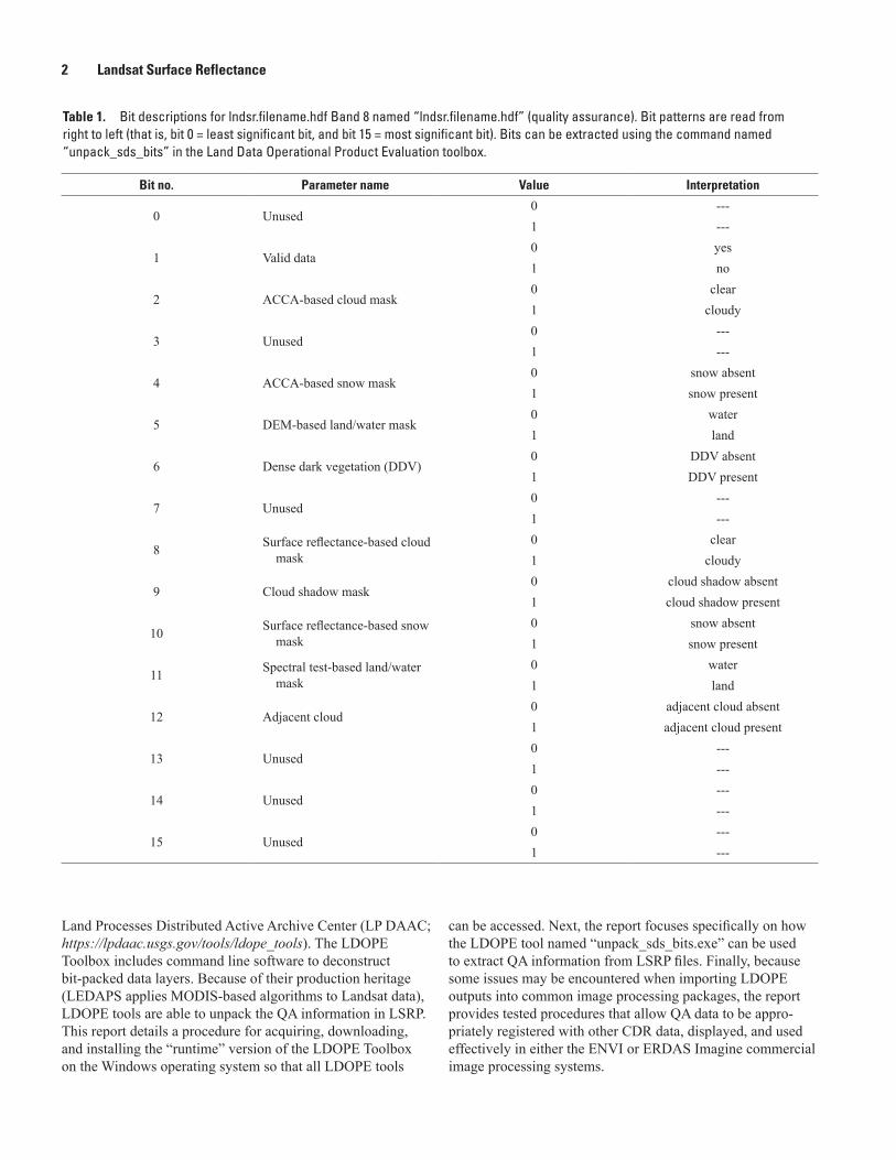
The QA definitions for LSRP are written to Band 8 named “lndsr_QA” (beginning with an “l” as in “landsat”), and a legend for interpretation of their unpacked values is shown in table 1.

A set of software tools to manipulate MODIS data was developed by the Land Data Operational Product Evaluation (LDOPE) team and are distributed at no cost from the NASA

1 U.S. Geological Survey, Reston, Va.2 U.S. Geological Survey, Rolla, Mo.3 Earth Resources Technololgy, Inc., Laurel, Md.

2 Landsat Surface Reflectance

Table 1. Bit descriptions for lndsr.filename.hdf Band 8 named “lndsr.filename.hdf” (quality assurance). Bit patterns are read from right to left (that is, bit 0 = least significant bit, and bit 15 = most significant bit). Bits can be extracted using the command named “unpack_sds_bits” in the Land Data Operational Product Evaluation toolbox.

Bit no. Parameter name Value Interpretation

0 Unused 0 --- 1 ---

1 Valid data 0 yes 1 no

2 ACCA-based cloud mask 0 clear 1 cloudy

3 Unused 0 --- 1 ---

4 ACCA-based snow mask0 snow absent1 snow present

5 DEM-based land/water mask 0 water 1 land

6 Dense dark vegetation (DDV) 0 DDV absent 1 DDV present

7 Unused 0 --- 1 ---

8 Surface reflectance-based cloud mask

0 clear 1 cloudy

9 Cloud shadow mask 0 cloud shadow absent 1 cloud shadow present

10 Surface reflectance-based snow mask

0 snow absent 1 snow present

11 Spectral test-based land/water mask

0 water 1 land

12 Adjacent cloud 0 adjacent cloud absent 1 adjacent cloud present

13 Unused 0 --- 1 ---

14 Unused 0 --- 1 ---

15 Unused 0 --- 1 ---

Land Processes Distributed Active Archive Center (LP DAAC; https://lpdaac.usgs.gov/tools/ldope_tools). The LDOPE Toolbox includes command line software to deconstruct bit-packed data layers. Because of their production heritage (LEDAPS applies MODIS-based algorithms to Landsat data), LDOPE tools are able to unpack the QA information in LSRP. This report details a procedure for acquiring, downloading, and installing the “runtime” version of the LDOPE Toolbox on the Windows operating system so that all LDOPE tools

can be accessed. Next, the report focuses specifically on how the LDOPE tool named “unpack_sds_bits.exe” can be used to extract QA information from LSRP files. Finally, because some issues may be encountered when importing LDOPE outputs into common image processing packages, the report provides tested procedures that allow QA data to be appro-priately registered with other CDR data, displayed, and used effectively in either the ENVI or ERDAS Imagine commercial image processing systems.

Software Installation and Setup 3

Data Access and AcquisitionThe currently provisional LSRP data collections

are accessible through a nominal user interface hosted at http://landsat.usgs.gov/PLSRP.php, which provides general product characteristics and a link to the ordering system. Users must submit a list of the Landsat scenes desired for surface reflectance processing in text format, as well as an electronic mail address for notification of order status and completion. A USGS-supplied user name and password is required to request and retrieve data products. To request account information, complete the “Contact Us” form on the LSRP Web site, select-ing the topic named “Surface Reflectance Data Request.”

Software Access and AcquisitionThe LDOPE Toolbox is provided at no cost to the user

through the NASA Land Processes Distributed Active Archive Center (LP DAAC) operated at USGS EROS. The user must establish a username and password (at “Sign Up”) before the software can be downloaded. Both the account establish-ment and download can be accomplished from this URL: https://lpdaac.usgs.gov/tools/ldope_tools.

Software Installation and SetupThe assumption is made that the necessary user account

has been established, and that the zip file named “LDOPE_Win_bin.zip” has been downloaded to the user’s local Win-dows desktop computer. It is also assumed that uncompression software, such as WinZip, is available on the desktop. Note: Administrator rights may be required to fully accomplish step 3.

Note as well that the following instructions are an adapta-tion and expansion of the procedures described in appendix D of the LDOPE_Users_Manual.pdf file:1. Make the directory where the software will be installed

and operated. For example, create a directory called “ESPA_QA” on the C drive.

2. Unzip the file named “LDOPE_Win_bin” and place the subdirectories it contains into the directory created above.Those subdirectories are named “bin” and “ANCIL-

LARY.” The bin subdirectory contains the executables and the ANCILLARY subdirectory contains numerous files used in map projection and georeferencing. Given the current exam-ple, a directory structure similar to that shown below should be present on the local disk:

C:\ESPA_QA

C:\ESPA_QA\ANCILLARY

C:\ESPA_QA\Bin

3. Create a new environment variable named “$ANCPATH“ (Windows XP shown first, followed by Windows 7 steps).This variable will point to the location of the ancillary

files in the new directory with subdirectories of LDOPE_Win_bin/ANCILLARY. To accomplish this in Windows XP, follow the steps below:

A. Click the Windows “start” button.

B. Select the control panel.

C. Click on the “systems” icon.

D. In the systems window, select the advanced tab.

E. In the advance window, select the button labeled ”Environment Variables.”

F. In the panel labeled ”User variable for username,” click on the button labeled “New.”

G. For the box labeled ”Variable name:,” enter the name “ANCPATH.”

H. For the box labeled ”Variable value:,” enter the value named “yourchoice/ANCILLARY” where ”yourchoice” is the directory created to hold the ANCILLARY and bin directories. In the case of the current example, “yourchoice” would be named “ESPA_QA” and the complete environment path would be “ESPA_QA/ANCILLARY.” (Note: The forward slash “/” is used.)

I. To avoid having to stipulate the path to the execut-able command each time it is run, add the path to the bin directory (that is, “yourchoice/bin”) to the environment variable named “$path.” Instructions for this process (for most operating systems) can be found here: http://java.com/en/download/help/path.xml. If this path is not configured, input files must be copied to the directory named “yourchoice/LDOPE_Win_bin” or the path to the command (for example, “yourchoice/LDOPE_Win_bin/”) must be specified from within the directory where the input data are found and output data will be placed. This latter case (specifying the path to the executable) is used in the example in step 4 below.

To create a new environment variable in Windows 7, fol-low the steps below:

A. Click the Windows “start” button.

B. Select the control panel.

C. Click on the “system” icon.

D. In the systems window, select “advanced systems settings.”

4 Landsat Surface Reflectance

E. In the window that pops open, select the tab named “Advanced.”

F. Click on the button labeled “Environment Vari-ables…”

G. In the panel labeled ”User variable for username,” click on the button named “New.”

H. For the box labeled “Variable name:,” enter “ANC-PATH.”

I. For the box labeled ”Variable value:,” enter “your-choice/ANCILLARY” where “yourchoice” is the directory created to hold the ANCILLARY and bin directories. In the case of the current example, “yourchoice” would be “ESPA_QA” and the complete environment path would be “ESPA_QA/ANCILLARY.” (Note: The forward slash “/” is used.)

J. To avoid having to stipulate the path to the execut-able command each time it is run, add the path to the bin directory (that is, “yourchoice/bin”) to the “$path” environment variable. Instructions for this process (for most operating systems) can be found here: http://java.com/en/download/help/path.xml. If this path is not configured, input files must be copied to the “yourchoice/LDOPE_Win_bin” directory or the path to the command (for example, “yourchoice/LDOPE_Win_bin/”) must be specified from within the directory where the input data are found and output data will be placed. This latter case (specify-ing the path to the executable) is used in the example in step 4 below.

4. Modify the command prompt “windowsize” to properly display LDOPE tool instructions and outputs in either XP or Windows 7.The LDOPE commands were written to run on an operat-

ing system that uses a wider “screen” than the 80-character one provided by default for the disk operating system (DOS) command prompt in current Windows operating systems. This results in difficult-to-read formatting for help and processing messages. To overcome this, the size of the command prompt window can be changed to make LDOPE help and output easier to read, using the following steps:

A. Open a command prompt window by either clicking on “start/run,” typing “cmd,” and clicking on “OK,” or at the “start/programs/accessories/command” prompt.

B. Click on the “c:\” icon in the upper left corner of the command prompt window that just opened.

C. Select “properties.”

D. Select “layout.”

E. Increase the screen buffer size to a width of 100.

F. Increase the window size to a width of 100.

G. Select “OK.”

H. Note: If using Windows XP, the prompt named “Save properties for future windows with the same title” must be toggled on before clicking “OK” if you want to retain the new command window size for all subsequent times it is used; otherwise just click “OK.”

Running the Command Named “unpack_sds_bits”

The “unpack_sds_bits” tool decodes the requested bit fields in the input file and writes them to an output HDF file for further processing. As per the documentation found at http://landsat.usgs.gov/PLSRP.php, each bit is coded with “1” or “0” (“yes” or “no,” respectively) values for various quality themes such as land, water, clouds, cloud shadow, and so forth. In the current example, this tool is being applied specifically to unpack two bit fields containing information on potential cloud and cloud shadow locations. The cloud masks produced through the Landsat Automated Cloud-Cover Assessment (ACCA) method and the cloud shadow mask are flagged in bits 2 and 9, respectively.

A. Use the existing or open a command window (“start/all programs/accessories/command” prompt or start/run and type “cmd”).

B. At the command prompt in the window, change directories to the location of the input data. For example, if LSRP data are in a directory called “testdata,” the following command would be issued: cd c:\testdata.

C. Unless the path to the bin subdirectory was added to the system path, it must be included when issuing each LDOPE tool command. For example, from within the testdata directory on the “C” partition a command is run to test that environment variables were properly set (steps 2G and 2H above), and to see what options are possible for the unpack_sds_bits command. In the current example, the LDOPE Toolbox was unzipped in the directory path named “ESPA_QA.” Therefore, at the command prompt, the following command is issued:

C:\ESPA_QA\bin\unpack_sds_bits –h.

This will display a page listing of options—inputs and outputs associated with the command (more eas-ily read if the command window width was modified as instructed in the previous section).

Adding QA Data to ENVI 5

D. Note that for LSRP data, the QA information is packed in the Science Data Set (SDS) or “band” that is named “lndsr_QA” (beginning with an “l” as in “landsat”).

E. For this example, the input LSRP file with a name of “lndsr.L5019037_03720010705.hdf” was collected via Landsat 5 for path 19 row 37 on July 7, 2001, and given an output file name of “2001_07_05_P19_R37_TM5_clds.hdf.”

The following command string would be issued (all on one line) to unpack both the ACCA-based and the surface reflectance-based cloud masks, as well as the LSRP cloud-shadow mask into the output file, assuming the input file is present in the directory named “ldope_win_bin\bin”:

c:\ESPA_QA\ldope_win_bin\bin\unpack_sds_bits –sds=lndsr_QA –bit=2,8,9 –of=2001_07_05_P19_R37_TM7_clds.hdf lndsr.L5019037_03720010705.hdf

The result is an output HDF file (named “2001_07_05_P19_R37_TM5_clds.hdf”) with three SDS, or bands, of data: the two-cloud and the cloud-shadow masks. This can be read by some software packages (for example, ENVI) as a three-band HDF file that will have a value of “1” in the first band for every pixel labeled as “cloud” by the ACCA algorithm, a value of “1” in the second band for every pixel labeled as “cloud” by the surface reflectance-based algorithm, and a value of “1” in the third band for every pixel labeled as cloud shadow by LSRP processing. The unpack_sds_bits command can be used

to similarly unpack any other QA bit (for example, bit 10 sur-face reflectance-based snow mask, bit 11 spectral-test-based land/water mask, and so forth) simply by changing the options provided for the “-bit” parameter. Additional bits can be added and separated by commas. For example, the option string–—bits=2,9,10—would result in a three-band output file in which the third band includes a “1” for every pixel labeled as “snow present” by LSRP processing.

Adding QA Data to ENVIAt the time this report was created, georeferencing infor-

mation embedded in the HDF file produced by the unpack_sds_bits command is not interpreted when the file is read as an HDF by the ENVI image processing system. That is, while the binary data can be read and displayed, their georeferencing information is “lost.”

Caution: While a LDOPE executable tool (named “cp_proj_param”) is designed to embed georeferencing information in the HDF file created by the unpack_sds_bits tool, it only operates properly in the case of MODIS HDF files and should not be used to overcome the problem of missing georeferencing in the QA extractions imported to ENVI. How-ever, the output of the unpack_sds_bits tool can be combined through ENVI commands with the LSRP reflectance bands so that they assume the georeferencing of the other layers and are properly and spatially aligned with those other layers.1. Load both the original ESPA HDF file and the file output

from the unpack_sds_bits command into ENVI. In the example below (fig. 1), the surface reflectance (SR) file

Figure 1. Screen capture showing that band names have been edited to reflect their content in the “Available Bands List” and the selection of the ENVI “Pixel-Based Mosaicking” tool (for compiling files).

Figure 2. Screen capture showing that the files already loaded in ENVI must be imported into the mosaicking tool.

6 Landsat Surface Reflectance

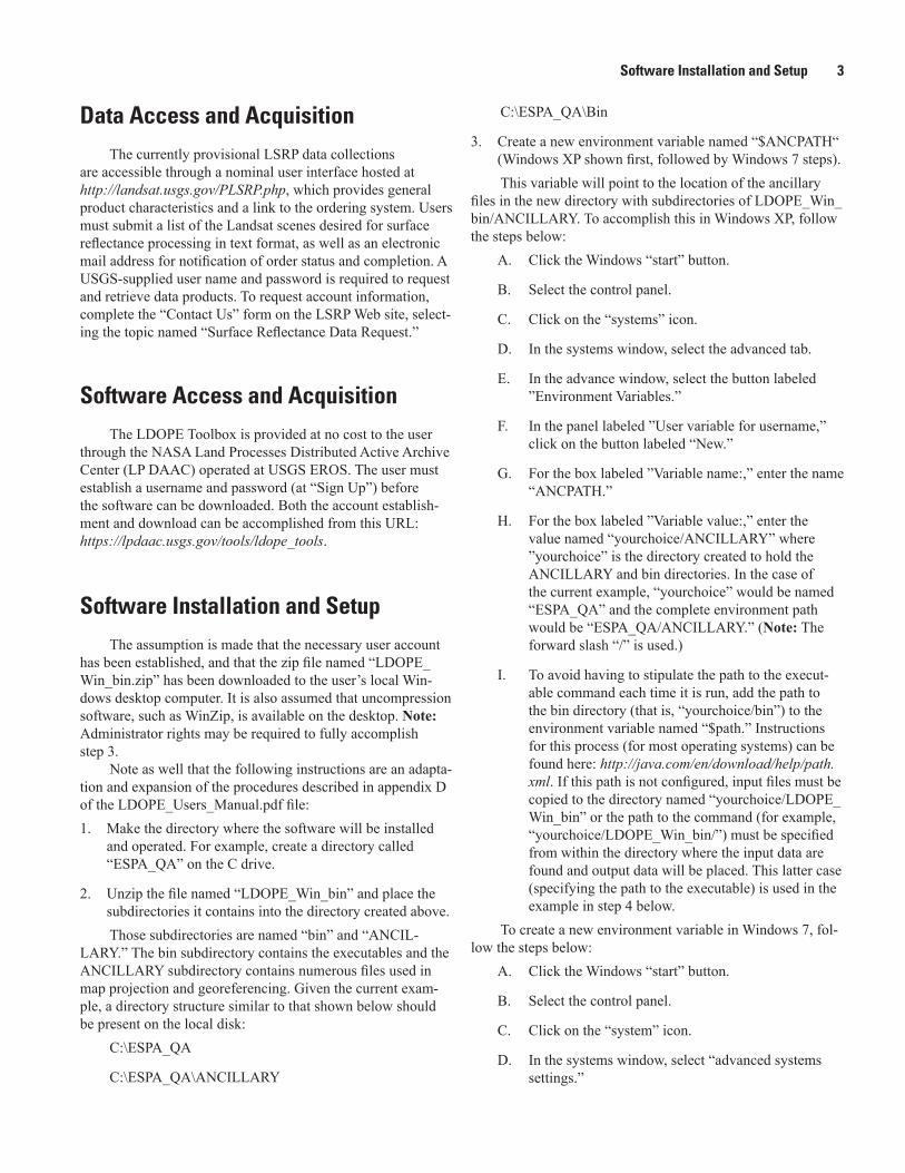
Figure 3. Screen capture showing the display of a cloud mask on top of the other band layers as a result of importing in sequence in ENVI.

has been loaded and its header was edited so that the band names indicate the content of each SDS (band) in the original file.

2. Use the ENVI “Pixel Based Mosaicking” tool to compile the files (fig. 1).

3. Import both files to the mosaicking tool in sequence (for example, SR first, cloud-shadow mask second) so that the cloud and shadow masks will be appended as the final two bands in the output file (figs. 2, 3, and 4).

When complete, either edit the band file names of the output or import an ASCII text file containing them; this is recommended for repeat or batch processing.

Adding QA Data to ERDAS ImagineThe QA data stored within Band 8 of the Surface Reflec-

tance HDF file can also be accessed using ERDAS Imagine software without using the LDOPE utilities. The following steps demonstrate the technique using ERDAS Imagine (ver-sion 10.1) with the classic interface. Note: When using this process, the extracted layers will be in reverse order of their listing in the original input file.1. Subset the QA band out of the Landsat Surface Reflec-

tance HDF file.

Figure 4. Screen capture showing the designation of an output file name and the specification of the background value (that is, parameter editing) in ENVI.

To isolate the band named “lndsr_QA” from and LSRP file in ERDAS Imagine, begin from the top level Data-Prep menu. Using the “Subset Image” option, select the LSRP HDF file as input, specify an output file (Imagine file format), and choose only Band 8 in “Select Layers” (fig. 5).

2. Export the QA subset file to generic binary.

From the top level “Import” menu, click the “Export” option. Choose “Generic Binary” in the “Type” dropdown menu to define the output file format. Select the LSRP Band 8 (QA subset) file created in step 1 as input, and specify an output filename (fig. 6).

Default values can be used for the export to Generic Binary format.

3. Import the generic binary file back into an ERDAS Imag-ine file.

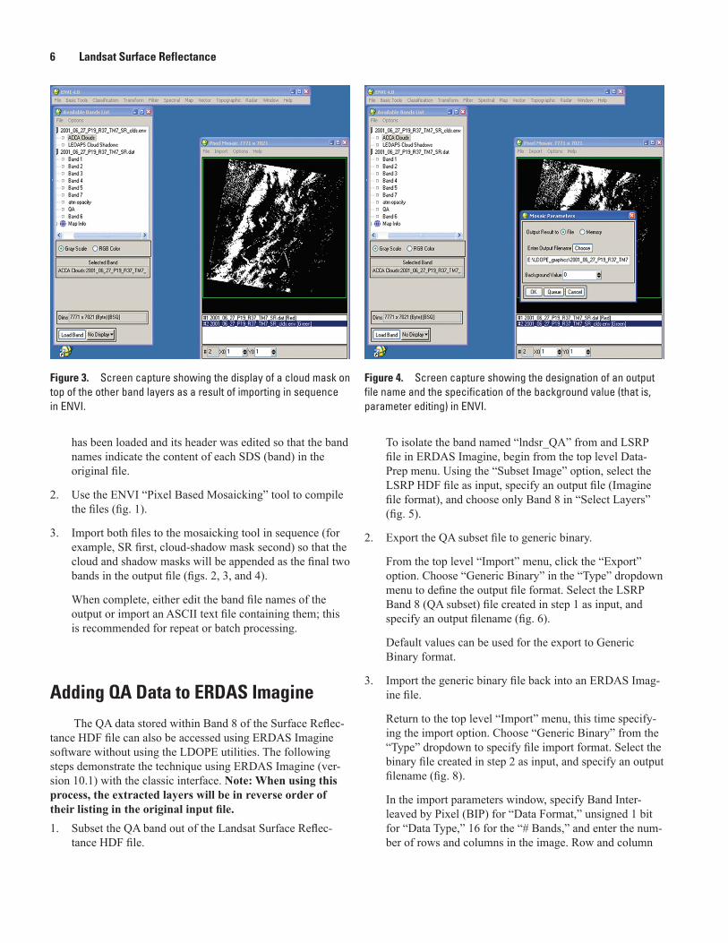
Return to the top level “Import” menu, this time specify-ing the import option. Choose “Generic Binary” from the “Type” dropdown to specify file import format. Select the binary file created in step 2 as input, and specify an output filename (fig. 8).

In the import parameters window, specify Band Inter-leaved by Pixel (BIP) for “Data Format,” unsigned 1 bit for “Data Type,” 16 for the “# Bands,” and enter the num-ber of rows and columns in the image. Row and column

Adding QA Data to ERDAS Imagine 7

information can be found using ImageInfo on the original HDF file (fig. 9).

4. Apply the georeferencing information to the resulting image.

Using ImageInfo on the original HDF file, find the coordi-nate values for the upper left “x” and upper left “y” pixel, the pixel size (should be 30 meters in these applications), and projection information.

Apply these values to the image created in step 3 using ImageInfo edits. First, under the “Edit” tab, select “Change Map Model,” and enter the upper left pixel coor-dinates, pixel size, units, and projection (fig. 10).

Then, under the “Edit” tab again, select “Add/Change Projection,” and specify the spheroid and datum names and the Universal Transverse Mercator (UTM) zone num-ber (fig. 11).

5. Viewing the QA bit layers.

The QA bit layers can be displayed in ERDAS Imagine in several ways. In the example below, the QA layers are displayed as a grayscale image with 16 bands, using “Raster-Band Combinations” to select which band (QA bit) is displayed (fig. 12). In this example, the spectral-test-based land/water mask (bit 11) is displayed (layer 5 in ERDAS Imagine).

The individual bit values for each QA bit can be viewed simultaneously per pixel using the “Start/Update Inquire Cursor” tool in the Viewer (fig. 13). QA bits 0 through 15 are displayed on separate rows in the cursor window: Lay-ers 1–16 correspond to bits 15–0 (that is, layer 10 displays the value for bit 6).

Figure 5. Screen capture showing the use of the ERDAS “Subset Image” option.

Figure 6. Screen capture showing the use of the ERDAS “Export” option (see fig. 7).

8 Landsat Surface Reflectance

Figure 7. Screen capture showing how to define the ERDAS output file format.

Figure 8. Screen capture showing the appropriate file type and media parameter to use when importing the output of the previous step in ERDAS.

Figure 9. Screen capture showing the selection of BIP and unsigned 1 Bit as the parameters to use as part of the processing in ERDAS.

Figure 10. Screen capture showing the use of ERDAS “ImageInfo” to apply the georeferencing information to the resulting image.

Reference Cited 9

Figure 11. Screen capture showing the specification of the spheroid and datum names and the Universal Transverse Mercator (UTM) zone number.

Figure 12. Screen capture showing display of spectral-test-based land/water mask (bit 11; layer 5 in ERDAS).

Figure 13. Screen capture showing view of the individual bit values for each quality assurance (QA) bit.

Reference Cited

Masek, J.G., Vermote, E.F., Saleous, N.E., Wolfe, Robert, Hall, F.G., Huemmrich, K.F., Gao, Feng, Kutler, Jonathan, and Lim, T.K., 2006, A Landsat surface reflectance dataset for North America, 1990–2000: Institute of Electrical and Electronics Engineers Geoscience and Remote Sensing Let-ters, v. 3, no. 1, p. 68–72.

Jones—Landsat Surface Reflectance Q

uality Assurance Extraction (Version 1.7)—

Techniques and Methods 11–C7