Contents lists available at SciVerse ScienceDirect
Landscape and Urban Planning
jou rn al h om epa ge: www.elsev ier .com/ locate / landurbplan
esearch paper
odeling the urban landscape dynamics in a megalopolitan cluster area byncorporating a gravitational field model with cellular automata
hunyang Hea,∗, Yuanyuan Zhaob, Jie Tianc, Peijun Shia
State Key Laboratory of Earth Surface Processes and Resource Ecology, Beijing Normal University, Beijing 100875, ChinaCollege of Resources Science & Technology, Beijing Normal University, Beijing 100875, ChinaDepartment of International Development, Community, and Environment, Clark University, 950 Main Street, Worcester, MA 01610, United States
i g h l i g h t s
This paper proposes a new megalopolis landscape dynamic model by combining a gravitational field model with a CA model.The model proposed produced more accurate simulation results than the CA model, which did not account for urban flows.The model proposed is of great value for locating ‘hotspots’ of future urbanization in a megalopolis cluster area.The model proposed can provide valuable information for regional landscape planning and environmental management in a megalopolis cluster area.
r t i c l e i n f o
rticle history:eceived 23 April 2012eceived in revised form 13 January 2013ccepted 14 January 2013
eywords:eijing–Tianjin–Tangshan megalopolitan
a b s t r a c t
The effective modeling of the urban landscape dynamics in a megalopolitan cluster area (MCA) is essen-tial to understanding its spatial evolution process. However, existing urban landscape dynamic modelsbased on cellular automata (CA) are limited in that they do not consider urban flows (e.g., flows of peo-ple, material, and information) between the different cities/towns in an MCA. This paper proposes a newmegalopolitan landscape dynamic model (MLDM) that is better suited for simulating the urban land-scapes in an MCA by combining a gravitational field model (GFM) with a CA model. The GFM was used to
model the influence of inter-city urban flows and to refine the transition rules of the CA model. The MLDMwas applied to simulate the urban landscape in the MCA of Beijing–Tianjin–Tangshan, and produced moreaccurate simulation results than the CA model that did not account for urban flows. The MLDM-basedprediction of future landscapes suggested that urbanization will continue in the region through 2020,especially in a few ‘hotspot’ areas. Close attention should be paid to these areas for strategic regionalplanning and environmental protection in this heartland of China.
. Introduction
The term megalopolitan cluster area (MCA) refers to a regionomprising a considerable number of cities clustered aroundhe regional economic core of one or two super-large cities.lthough these cities can significantly differ one from another,
hey are closely interconnected and have strong interactions dueo the highly developed regional transportation and informationetworks (Lang & Knox, 2009; Yao, Chen, & Zhu, 2006). MCAsre often the most vigorously developing urban areas around the
orld and attract a great deal of attention (Gu, Hu, Zhang, Wang,
Guo, 2011; Tian, Jiang, Yang, & Zhang, 2011a; Vicino, Hanlon, Short, 2007). For example, the MCA of Washington–Baltimore,
Boston, Philadelphia, and New York covers only 1.4% of US ter-ritory but is home to 17.3% of the US population (Vicino et al.,2007). In China, the three major MCAs (Yangtze, Pearl RiverDelta and Beijing–Tianjin–Tangshan) comprise only 2.2% of thecountry’s territory but are home to 12% of the Chinese pop-ulation and contribute 34% of China’s gross domestic product(GDP) (NSBC, 2010). These MCAs have become highly urban-ized in the past decades, and the local natural landscapes havebeen removed or considerably changed. This urbanization pro-cess has resulted in enormous ecological and environmental issues,such as increased surface temperature and decreased biodiver-sity (Chen, Li, Zheng, Guan, & Liu, 2011; Foley, DeFries, & Asner,2005; Grimm et al., 2008; Jenerette & Wu, 2001; Nikanorov,Khoruzhaya, & Mironova, 2011; Valiela & Martinetto, 2007; Yang,
Hou, & Chen, 2011). Spatial process models are important tools forbetter understanding the driving forces to urban landscape dynam-ics and evaluating their ecological and environmental impacts(Valbuena, Verburg, Bregt, & Ligtenberg, 2010). There has been
great need for models that can effectively simulate the urbanandscape dynamics of MCAs to support the urban/regional plan-ing and the sustainable development in these areas (Berling-Wolff
Wu, 2004a; Wu & David, 2002; Wu, 2010).At present, the simulation of urban landscape dynamics mainly
elies on four types of models (Berling-Wolff & Wu, 2004a; Parker,anson, Janssen, Hoffmann, & Deadman, 2003). The first type
escribes urban structure and morphology in a qualitative way;ost models of this type were developed before the 1940s, includ-
ng concentric zone model, sector model, and multiple nuclei modelHe, Okada, Zhang, Shi, & Li, 2008). The second type is built uponewton’s theory of gravity, and focuses on depicting the spatial
nteractions between different entities. Typical examples includehe gravity model (Foot, 1981) and the Lowry model (Harris, 1985).he third type uses differential equations to represent the spatialrocess; the models of this type were initially proposed in the 1970sith the system dynamic models being representative (Gilbert &
roitzsch, 1999). The last type includes the discrete dynamic mod-ls that have flourished since the 1970s; the best known examplesnclude cellular automata (CA) (Santé, García, Miranda, & Crecente,010) and multi-agent system (Parker et al., 2003) models. CAodels have been widely applied to simulate urban landscape
ynamics in the past two decades (Berling-Wolff & Wu, 2004b; Het al., 2006a; He, Okada, Zhang, Shi, & Zhang, 2006b; He et al., 2008).umerous works have successfully demonstrated the capability ofA models in representing the complex process of urban landscapevolution (Barredo, Kasanko, McCormick, & Lavalle, 2003; Fang,ertner, Sun, & Anderson, 2005; Li & Yeh, 2002; Mitsova, Shuster,
Wang, 2011; Sui & Zeng, 2001). However, a CA model typicallyssumes that the regional pattern change is an aggregate of theocal changes, and simulates the evolution of an urban ecosystemased merely on local interactions (Qi et al., 2004). This approachocuses on micro individual cells and often neglects the links andnteractions between cells and the macro spatial patterns (Qi et al.,004). In addition, the ‘bottom-up’ construction of traditional CAodels usually prevents them from fully capturing the macro-scale
ocioeconomic driving forces of urban landscape dynamics (Ward,urray, & Phinn, 2000; White & Engelen, 1997; White & Engelen,
000). Therefore, researchers have attempted to extend andnhance traditional CA models by incorporating socioeconomicodels. For instance, White and Engelen (2000) linked a CA modelith a regional development model to simulate the evolution ofrban landscapes for the entire country of the Netherlands. Wund David (2002) integrated hierarchical theory with a CA modelo simulate the urban landscape dynamics in the metropolitanrea of Phoenix, AZ, USA. He et al. (2008) incorporated a potentialodel with a CA model to simulate the landscape dynamics in the
eijing metropolitan area. Most recently, Kuang (2011) coupled aA model with an artificial neural network model to simulate therban landscape changes in the Beijing–Tianjin–Tangshan region,hina. These researches have significantly enhanced the ability ofA models to accurately simulate landscape dynamics in an urbanrea.
However, most of the existing models are focused on one singleity and not suitable for modeling the urban landscape dynamics inn MCA. In order to solve this problem, Li and Liu (2006) proposedn extended CA model in which the transition rules were deter-ined by using a case-based reasoning (CBR) technique. The idea is
o build a case library based on the geographical data including landse/cover, and then determine the state of a cell state according tohe proximity between the cell and the cases in the library calcu-ated. The advantages of this model include not having to define the
ransition rules and being possibly able to simulate for complex sit-ations. The disadvantages include: (1) the model accuracy is highlyensitive to the representativeness of the case data; (2) the model,
Planning 113 (2013) 78– 89 79
once established, may not be effectively applied to a different studyarea; and (3) the physical meaning of the model is not so clear.
Urban flow refers to the frequent interflows of people, mate-rial, information, capital, and technologies among a cluster ofcities/towns (Zhu & Yu, 2002). There exists a variety of trans-portation networks including highways, expressways, waterwaysand airways within and between the urban areas in an MCA. Thesocio-economics of the cities/urban areas of different sizes stronglyinteract with each other, collectively driving the regional develop-ment of an MCA. Therefore, urban flows often play a significant rolein the evolution of an MCA (Gu et al., 2011; Limtanakool, Schwanen,& Dijst, 2007; Seto & Fragkias, 2005). Urban flow intensity char-acterizes the strength of the influence from the centralizationand decentralization of the cities in an MCA. Zhu and Yu (2002)defined the concept of urban flow intensity and used it in analyz-ing the urban flows in the HuNingHang megalopolitan cluster. Caoand Wang (2007) analyzed the intensity of the urban flows in acity cluster of Northeast China. These studies have suggested thaturban flow intensity is an effective indicator of the strength of thesocioeconomic interactions between the member cities/towns ina megalopolitan cluster area (Derudder & Taylor, 2005; Yao et al.,2006).
The gravitational field model (GFM) was first proposed byLagrange in 1773 to measure the gravitational influence of a planetfrom a distance (Stewart, 1947). In the 1940s, Stewart adopted theGFM to represent the influence of population as a function of dis-tance and applied it for the first time in socioeconomic research(Brown, 1982; Gardiner, Martin, & Tyler, 2011; Stewart, 1941,1942, 1947). In the 1980s, Friedman (1986) treated an MCA as anurban field in which the spatial influence of one city on anotheris inversely related to the distance between them. Liang (2009)employed the GFM to calculate the local/regional impact of 670Chinese cities with non-agricultural populations exceeding 80,000.Wu, Zhang, Jin, & Deng (2009) used a GFM to study the spatialinteractions among 18 cities in the coastal area of eastern Chinaduring 1991–2002, by analyzing the economic, population, andtransportation data. Most recently, Wang, Deng, Liu, & Wang (2011)used a GFM to investigate the urban expansion in central China from1990–2007. These studies have shown that GFMs are effective inrepresenting the spatial interactions among cities. However, a GFMalone is inadequate for representing the complex spatial processesof the urban landscape evolution in an MCA because it cannot wellcapture the micro-scale dynamics.
This paper presents a new megalopolitan landscape dynamicmodel (MLDM) that can better model the urban landscape dynam-ics in MCAs. The model basically integrates a GFM with a CA model.In the MLDM, the demand for urban land in an MCA is first esti-mated based on the socioeconomic data. Then, a GFM is employedto model the urban flows within the MCA. Next, the GFM is incor-porated in defining the transition rules of a CA model to moreaccurately map the potential new urban cells that are to meetthe urban land demand of the MCA. A case study was conductedby applying the model to simulate the urban landscape dynamicsin the Beijing–Tianjin–Tangshan megalopolitan cluster area (BTT-MCA) of China for the time period of 1990–2009 and to predict the‘hotspot’ areas that are highly likely to experience rapid urbaniza-tion from 2009 to 2020.
2. Description of the MLDM
The objective of the MLDM is to consider not only the evolution
of individual land cells, but also urban flows between the differ-ent cities/towns in an MCA. Landscape dynamics in an MCA canbe regarded as a self-organizing process influenced by broad-scaleenvironmental, geographical, and socioeconomic factors (Barredo
80 C. He et al. / Landscape and Urban
Core city
Sub -core city
Major city
Other cities
Influence of urban flows beyond the
neighborhood (arrow thickness
represents the urban flows of cities at
different hierarchical levels)
Non-urban landscape occupied in the
process of urban landscape evolution
Urban landscape
Road
Neighborhood
space
Fig. 1. The conceptual model.
eofctwmft
feauo
iby Zhu and Yu (2002) and Yao et al. (2006), Fi can be calculated asfollows:
Fi = Ni × Ei (2)
t al., 2003; He et al., 2008). The MLDM assumes that the evolutionf the urban landscape in an MCA is shaped by the regional demandor urban lands and the potential conversion of a non-urban landell to an urban cell is co-determined by local neighborhood fac-ors (from a CA model perspective) and the inter-city urban flowsithin the MCA. The model therefore integrates a GFM with a CAodel so that the influence of urban flows can be modeled by the
ormer while that of local neighborhood factors can be modeled byhe latter (Fig. 1).
The MLDM consists of three parts: (1) the estimation of demandor urban land in an MCA; (2) a GFM-based definition of the influ-nce of inter-city urban flows on the urban landscape evolution;nd (3) the prediction of future urban land cells by considering therban flow influence defined in (2) in framing the transition rulesf the CA model (Fig. 2).
Population
Economy
Regional factors
Statistical model
Urban landscape demand
Urban flow influence
Urban landscape dynam
Driving for
Urban flow of core cities
Urban land area Urba
Urban flow of sub-core cities
Urban flow of major cities
Gravational
field model
Urban flow of other cities
Demand-supply
balance
Fig. 2. Flowchart of the megalopolit
Planning 113 (2013) 78– 89
2.1. Estimating the demand for urban land
At present, several non-spatial models are available for estimat-ing the demand for urban land in an MCA during a given time period,including the linear programming model (Wang, Yu, & Huang,2004), the regression analysis models (López, Bocco, & Mendoza,2001; He et al., 2008), and the system dynamic models (He et al.,2006a,b). The regression analysis models are merited for the rel-atively simple calculations and fewer parameters required. Lópezet al. (2001) suggested that the population residing in an urban areais highly correlated with its size. Therefore, historical data on thesize of an urban area can be regressed on its population and theregression model can be further used to predict the future demandfor urban land based on population growth data. Please refer tosection 3.4 for further details.
2.2. Defining the influence of urban flows on landscape evolution
As discussed by Liang (2009) and Wang et al. (2011), an MCAcan be regarded as a field of urban flow intensity, which decreasesover distance from the city centers. We adopted this concept andused the GFM to quantify the influence of urban flows on the land-scape evolution in an MCA. According to Liang (2009), the influenceof urban flows on a non-urban cell (x, y) at time t (t Ii,x,y) can beexpressed as follows:
t Ii,x,y = Fi
D(x,y,xi,yi)(1)
where t Ii,x,y is the intensity of the urban flow from city i at cell (x,y); D(x,y,xi,yi) is the Euclidean distance from the city center (xi, yi) tothe cell (x, y); and F is the urban outflow from city i. As suggested
Local driving forces
Inherited attribute
Ecological constraints
Local factors
Cellular automata model
Urban landscape supply
ics
ces Resistant forces
Suitability
Neighborhood
effect
n land location
an landscape dynamic model.
Urban
watars
E
wcfi
E
wiiMtahptcovj
o2(b
I
2
abbMtl
a
t
wtr
t
wtTa
t
wcc
C. He et al. / Landscape and
here Ni stands for the internal function (the ability of city i inn MCA to support itself), which can be fairly well represented byhe city’s GDP per employee. Ei denotes the external function (thebility of city i to support other cities in the MCA), which can beepresented by totaling the external functions of all the economicectors of city i as follows (Yao et al., 2006; Zhu & Yu, 2002):
i =m∑
j=1
Eij (3)
here Eij is the output function of a specific economic sector (j) ofity i, and m is the number of sectors in city i. Eij is calculated asollows because it is effective and the data required to calculate fort are usually available:
ij = Gij − Gi × Gj
G(4)
here Gij is the number of employees in economic sector j of city, Gi is the number of employees in all the economic sectors of city, Gj is the number of employees in economic sector j of the entire
CA, and G is the total number of employees of the MCA. If Eij ≤ 0,he economic sector j of city i has no output function and Eij is given
value of 0. If Eij > 0, it means that the economic sector j of city ias an output function for the other cities in the MCA because theroportion of employees in the sector j of city i is larger than that ofhe entire MCA. In other words, the sector j is more centralized inity i than the other cities/towns in the MCA and therefore has anutput function to support the other cities in the MCA. A larger Eijalue indicates a stronger output function for the economic sector
of city i (Yao et al., 2006).When a land cell is influenced by the urban flows from cities
f similar sizes, the maximum influence is accounted (Wang et al.,011). Thus, for a non-urban cell (x, y), the urban flow influenceIk,x,y) from a number (s) of cities with a comparable size of k, cane expressed as:
According to Barredo et al. (2003), He et al. (2008) and Whitend Engelen (2000), the urban landscape evolution in an MCA cane understood as a complex process determined simultaneouslyy driving forces, resistant forces, and random perturbation. In theLDM, the driving forces primarily include: (1) land suitability, (2)
he contextual effect of a local neighborhood, and (3) the macro-evel urban flows from the different cities in an MCA.
The probability tPx,y for cell (x, y) to be converted into urban uset time t can be expressed as:
Px,y = f (tDx,y, tRx,y, tVx,y) (6)
here tDx,y, tRx,y, and tVx,y represent the driving forces, resis-ant forces, and random perturbation influencing the land change,espectively. tDx,y can be further expressed as:
Dx,y = f (tSx,y, tNx,y, t Ix,y) (7)
here tSx,y stands for the suitability, and tNx,y and t Ix,y representhe neighborhood effect and the urban flow intensity, respectively.he resistant force tRx,y can be considered a function of two vari-bles as follows:
R = f (t J , tEC ) (8)
x,y x,y x,y
here t Jx,y is the continuity attribute for cell (x, y) to maintain itsurrent land use or cover state (z) at time t. tECx,y is the ecologicalonstraint (e.g., located in an reservation area) that prevents a cell
Planning 113 (2013) 78– 89 81
(x, y) from being converted to urban use. The random perturbationterm tVx,y can be constructed as:
tVx,y = 1 + [− ln(rand)]a (9)
where rand (0 < rand < 1) is a random variable and a is an adjustableparameter representing the magnitude of the random perturba-tion. To keep the calculation manageable while incorporating urbanflows into the transition rule of a CA model, the probability tPx,y fora non-urban cell to be converted into an urban cell can then beexpressed as:
tPx,y =(
m−n∑i=1
Wi × tSi,x,y + Wm−n+1 × tNx,y
+m−1∑
i=m−n+2
Wi × t Ii,x,y − Wm × t Jx,y
)×∏r=1
tECr,x,y × tVx,y
(10)
where∑m−n
i=1 Wi ×t Si,x,y is the suitability for the conversion at timet. tSi,x,y is a standardized suitability score [0, 100] based on theconsideration of a number (i = 1, . . ., m – n) of factors. m is the totalnumber of weights and m – n is the number of suitability factors. Widenotes the weight associated with each factor. tNx,y represents theneighborhood effect for cell (x, y) at time t and Wm − n + 1 is its asso-ciated weight. The term
∑m−1i=m−n+2Wi ×t Ii,x,y quantifies the overall
urban flow influence from all the cities/towns in an MCA, in whicht Ii,x,y is the urban flow influence from the cities of a comparablesize k and Wi is the corresponding weight. t Jx,y is the continuityattribute of cell (x, y) and Wm is its weight. These weights (W1, W2,. . ., Wm) are used to represent the relative importance of the fac-tors that drive or resist urban landscape changes.
∏r=1
tECr,x,y is theproduct of a few binary variables used to represent the ecologicalconstraints on the urban landscape change, such as being locatedin an area of nature reserve or water protection. tECr,x,y will have avalue of 0 if cell (x, y) is preserved due to constraint r.
Neighborhood size is essential in running a CA model, as itshould well define the extent of interactions between land uses andthe scale of the land dynamics of an ecosystem (Caruso, Rounsevell,& Cojocaru, 2005). According to Barredo et al. (2003), He et al. (2008)and White and Engelen (2000), a neighborhood in the MLDM is acircular area around the cell of interest with a radius of five cells.This definition of neighborhood is believed to be appropriate forcapturing the local urban cells’ agglomeration effect (Chen, Gong,He, Luo, & Tamural, 2002). The neighborhood effect tNx,y can bequantified as:
tNx,y = A ×∑
c
tUc
C(11)
where tUc indicates whether a cell at the distance C from cell (x, y)is urban. tUc will have a value of 1 if it is urban and 0 if not. A is ascalar used to linearly standardize tNx,y into the range of [0, 100].
Once the probability tPK,x,y for cell (x, y) to be converted intourban use from a type z is determined, the evolution of the urbanlandscape can be simulated with respect to the total demand forurban land. To simplify the computation of the model, we can gen-erally classify the various land use types into urban and non-urban,and only model the conversion processes from one generalized typeto the other. Competition for space among different types of landuse does not need to be considered because almost all the consump-tion of non-urban lands in our study area is for urban development.
The simulation of the urban landscape dynamics in an MCA followsa repetitive computational workflow. tPK,x,y is calculated for eachcell, and the cell with the highest tPK,x,y value is labeled as a futureurban cell with high confidence. If the estimated total demand for
8 Urban
utu
3d
3
wr5BTiaNotlb
2 C. He et al. / Landscape and
rban land in the simulated period cannot be satisfied by changinghat cell into urban use, another iteration begins. The loop continuesntil the total area of urban land reaches the demand.
. Applying the MLDM to simulate the urban landscapeynamics in the BTT-MCA, China
.1. Study area and data
The study area of BTT-MCA is located in the North China Plainith a latitude range of 38◦28′ N to 41◦05′ N and a longitude
ange of 115◦25′ E to 119◦53′ E. It has a total spatial area of about5,774.5 km2 and accounts for 0.5% of the total area of China. TheTT-MCA consists of 43 cities and towns, including Beijing, Tianjin,angshan, Qinhuangdao, and Langfang (Fig. 3). Beijing is the cap-tal of China and the political and cultural center of the countrys well. Tianjin is the third largest city and the largest port city inorth China. Beijing and Tianjin are under the direct jurisdiction
f the central government, and are regarded as the ‘dual core’ ofhe BTT-MCA (Tan, Li, Xie, & Lu, 2005). In 2009, the urban popu-ation and the GDP of the BTT-MCA were 20.68 million and 2250illion Chinese Yuan, accounting for 6.61% and 3.33% of the totals for
Fig. 3. The stu
Planning 113 (2013) 78– 89
Mainland China, respectively (NSBC, 2010). Since China imple-mented its open-door policy in the 1970s, the BTT-MCA hasexperienced tremendous urbanization (Kuang, 2011; Tan et al.,2005).
A series of land use/cover maps (1990, 2000, and 2009) for theBTT-MCA were used in this study. All of these maps were pro-duced from the classification of Landsat TM/ETM+ images of goodquality and have six land use/cover classes (urban land, cropland,grassland, forest, water, and others). Socioeconomic data (e.g., pop-ulation, GDP, and number of employees in each economic sector)from the National Statistics Bureau of China (NSBC) were also col-lected and included in our modeling. A digital elevation model wasobtained from the International Scientific Data Service Platform(http://datamirror.csdb.cn/dem/files/ys.jsp, accessed 02.02.12) torepresent the regional topography, and a number of geographi-cal information system (GIS) data layers were also collected fromthe National Administration of Surveying, Mapping, and Geoin-formation of China, including administrative boundaries, rivers,road networks, city centers, airports, and coastal ports. All the GIS
data were georegistered to the Albers Conical Equal Area projec-tion and the raster datasets were resampled to have the samecell size of 300 m (1228 columns, 969 rows), which was suffi-cient to capture the detailed information about urban landscape
Core city Sub-core city Major cities Other citiesPro
po
rtio
n o
f u
rba
n p
op
ula
tio
n l
0%
5%
10%
15%
20%
25%
30%
35%
40%
Core city Sub-core city Major cities Other cities
Pro
po
rtio
n o
f G
DP
(a)
(b)
FB
d(
3B
c(Tdofqf
I
wIm
31
mttoduadtN
ig. 4. Socioeconomic discrepancies between the cities in theeijing–Tianjin–Tangshan megalopolitan cluster area in 2009.
ynamics while keeping the volume of computation manageableKuang, 2011).
.2. Calculating the influence of urban flows between cities in theTT-MCA, China
Based on their socioeconomic characteristics in 2009, the 43ities/towns in the BTT-MCA were classified into four categories:1) the primary core city of Beijing, (2) the secondary core city ofianjin, (3) the major cities of Tangshan, Langfang, and Qinhuang-ao, and (4) the other smaller cities and towns (Fig. 4). The influencef the urban flows from the cities in each category was calculatedrom the GIS data using Eq. (1). The influence values were subse-uently standardized into the range of [0, 100] using the followingormula and the resultant maps are displayed in Fig. 5.
s = I − Imin
Imax − Imin× 100 (12)
here Is is the standardized influence of an urban flow influence,min is the raw minimum influence value while Imax is the raw
aximum.
.3. Model calibration and urban landscape simulation from990 to 2009
Calibration and validation are critical for the performance of CAodels because it largely depends on the appropriateness of the
ransition rules, which typically involve several important parame-ers (Wu, 2002; Straatman, White, & Engelen, 2004). The calibrationf the MLDM is usually conducted based on reliable historicalata, which hopefully facilitates the effective simulation of futurerban landscape dynamics (Wu, 2002). However, the calibration
nd validation of urban CA models are in fact rather challengingue to the complexity of urban landscape evolution processes andhe numerous combinations of parameters involved (Verburg, Deijs, Ritsema van Eck, Visser, & De Jong, 2004). Progress has been
Planning 113 (2013) 78– 89 83
made for urban CA models with the development of two typesof calibration methods (Li & Yeh, 2002). One of them is based onmathematical and/or statistical analysis, such as logistic regression(Wu, 2002) and artificial neural networks (Kuang, 2011). The othertype are the trial and error approaches, including visual tests (Wardet al., 2000), landscape metrics comparisons (Berling-Wolff & Wu,2004b), and computer simulation comparisons (He et al., 2008).As suggested by Chen et al. (2002) and He et al. (2008), an adap-tive Monte Carlo approach was chosen to automatically calibratethe parameters in the MLDM. This approach is mainly driven bydata and avoids subjective determination of the weights used in thetransition rules of the CA model. Specifically, a Monte Carlo samp-ling process was used to search for the optimal combinations ofweights that resulted in the most accurate simulation results. Sinceall the weights in a transition rule should total to 1, the calibrationprocess can be expressed as follows:
Objective function max A(w1, w2, · · ·, wm) (13)
Constrained conditionm∑
k=1
wk = 1 (14)
where wk is the weight for factor k and A is a measure of agreementbetween the simulation result and the reality. We chose the kappaindex for A because it is widely recognized as an effective mea-sure of accuracy for remote sensing classifications. As suggested byChen et al. (2002) and He et al. (2008), up to 500 iterations wereconducted to achieve the best performance. Although the simula-tion was computationally intensive, it was manageable with thestrong computing power of our workstations.
The 2000 and 2009 urban land use maps were used to cali-brate the MLDM by treating the 1990 map as the starting point.Thirteen of the most important impact factors were incorporatedin the MLDM, including the influence of the urban flows from allthe four categories of cities, slope, distances to highways, railways,expressways, coastlines, airports, harbors, and city centers, neigh-borhood effect, and continuity attribute. Since it is understandablethat the influence of urban flows was dynamic, and therefore it wasmodeled for 1990, 2000 and 2009 in order to simulate the urbanlandscape change during 1990–2000, 2000–2009 and 2009–2020.Because these factors were measured in different units, they wereall scaled into the range of [0, 100]. Urban landscape dynamicswere simulated for the periods of 1990–2000 and 2000–2009, with500 different sets of weights for the 13 impact factors. The sim-ulated urban landscapes for 2000 and 2009 based on each set ofweights were compared with the actual urban landscapes in thesetwo years. The most accurate simulation results achieved a kappaindex value of 0.81 and 0.82 for 2000 and 2009, respectively.
The set of weights that produced the most accurate simula-tion results (Fig. 6) are displayed in Table 1. As suggested by Santéet al. (2010), the single use of Kappa index is not enough to assessthe urban spatial patterns generated by CA models. So we per-formed the further accuracy assessment of the simulated resultsusing Moran I index by referring to the relative works of Wu (2002)and Liu, Li, Liu, He, & Ai (2008b). It was found the Moran I valuesof the simulated urban pattern in 2000 and 2009 are 0.93 and 0.96,respectively, close to the actual urban pattern’s 0.97 and 0.99. Over-all, the simulation results by the MLDM matched the actual urbanlandscapes quite well, although some small-scale details were noteffectively captured. To assess their importance to the model, theinfluence of the urban flows was excluded from consideration ina test simulation for both periods. The highest kappa index val-
ues for the two year were both below 0.8, 0.75 and 0.78 for 2000and 2009, respectively. Meanwhile, their Moran I values are 0.89in 2000 and 0.93 in 2009, also more different to the actual’s 0.97and 0.99 than the simulated results with urban flow. The lower
84 C. He et al. / Landscape and Urban Planning 113 (2013) 78– 89
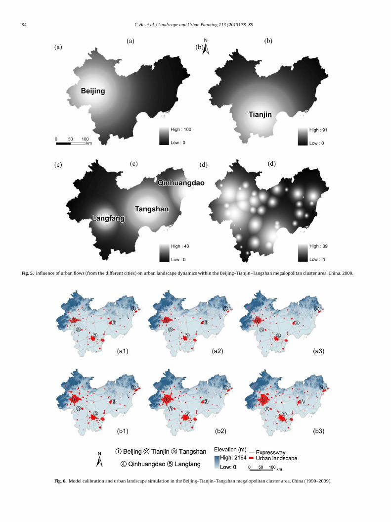
Fig. 5. Influence of urban flows (from the different cities) on urban landscape dynamics within the Beijing–Tianjin–Tangshan megalopolitan cluster area, China, 2009.
Fig. 6. Model calibration and urban landscape simulation in the Beijing–Tianjin–Tangshan megalopolitan cluster area, China (1990–2009).
C. He et al. / Landscape and Urban Planning 113 (2013) 78– 89 85
Table 1Calibrated weights for the periods of 1990–2000 and 2000–2009.
Factors Weights for 1990–2000 simulation Weights for 2000–2009 simulation
Slope 0.03 0.06Distance to highway 0.09 0.02Distance to railway 0.06 0.04Distance to expressway 0.01 0.12Distance to coastline 0.04 0.01Distance to airports and harbors 0.01 0.09Distance to city centers 0.05 0.02Urban flow influence of core city 0.09 0.1Urban flow influence of sub-core city 0.01 0.12Urban flow influence of major cities 0.04 0.05Urban flow influence of other towns 0.14 0.12Neighborhood effect 0.25 0.19
aiflttstutmutuvn
3
Mtf((
y
FB
Continuity attribute 0.18
ccuracy indicates the significance of accounting for urban flowsn the simulation. The simulations that do not account for urbanows tend to overestimate the roles of neighborhood effect andhe transportation networks in driving the urban landscape evolu-ion in an MCA. For example, the MLDM accounting for urban flowsuggested that, in 2000, newly converted urban lands were dis-ributed more around Beijing than around the other pre-existingrban areas [Fig. 6(a2)]. This is a much more accurate represen-ation of the actual situation than what was produced by the CA
odel that did not consider urban flows which showed a relativelyniform distribution of newly converted urban lands around allhe pre-existing urban areas [Fig. 6(a1)]. The MLDM accounting forrban flow influence also correctly suggested that the newly con-erted urban lands were mainly located around Tianjin and theortheast of Beijing in 2009 [Fig. 6(b2)].
.4. Prediction of urban landscape dynamics from 2009 to 2020
The ability to predict the future urban landscape in the BTT-CA is very important. In order to predict the future landscape in
he study area using the proposed MLDM, we first estimated theuture demand for urban land based on population growth data
1990–2009) for the BTT-MCA (Fig. 7). A linear regression modelEq. (15)) was built to predict urban population on year:
= 39.17x + 1257.27 (15)
y = 39.17 x + 1257.27
R 2 = 0.97
1000
1200
1400
1600
1800
2000
2200
0 2 4 6 8 10 12 14 16 18 20
Time
Urb
an
po
pu
latio
n (
10
,00
0s)
l
ig. 7. Linear regression of urban population on year in theeijing–Tianjin–Tangshan megalopolitan cluster area, China.
0.06
where y stands for the urban population and x stands for a yearrelative to 1990 (e.g., x = 6 for 1995). The regression was found tohave a very strong predictive power, with an r2 of 0.97.
Subsequently, another regression model (Eq. (16)) was devel-oped based on the historical data (1990–2009) on the urbanpopulation and the corresponding total area of urban land in theBTT-MCA (Fig. 8):
y = 3.27x − 3171.05 (16)
where y stands for the total area of urban land and x stands for thetotal urban population. This regression model was also found tohave a rather strong predictive power (r2 = 0.99).
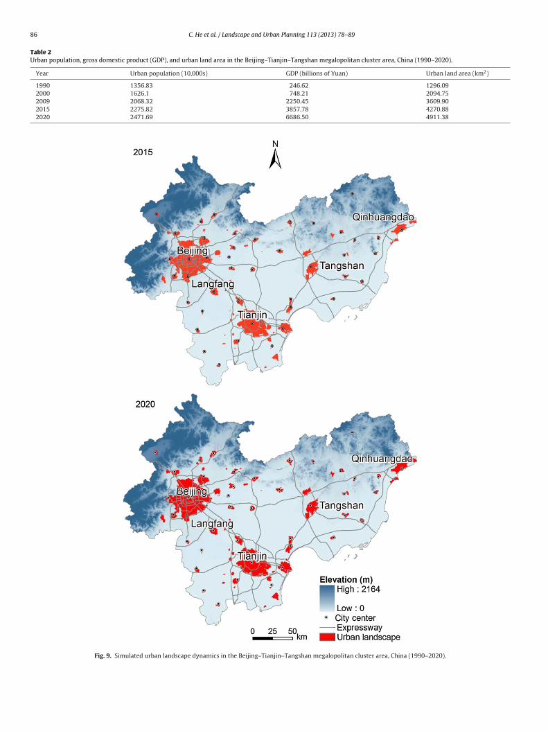
The historical and predicted data of urban population, GDP, andurban land area for the BTT-MCA are summarized in Table 2.
Future urban landscapes in the BTT-MCA were simulated for2009–2020 using the calibrated MLDM and the estimated futuredemand for urban land. Fig. 9 displays the simulated urban land-scapes for 2015 and 2020, which clearly suggest a continuingurbanization in the region. Fig. 10 highlights the areas in the BTT-MCA that are likely to be converted into urban use before 2020,mainly including the northeast of Beijing, the east of Tianjin, andthe outskirts of Langfang. Such foreseeable rapid urbanization inthe BTT-MCA may create or intensify environmental and ecolog-
ical problems, such as air pollution, biodiversity reduction, andlocal/regional climate change (Chen et al., 2002, 2011). Therefore,the highlighted areas deserve closer attention for a more effectivemanagement of this heartland of China.
y = 3.27 x –3171.05
R 2 = 0.99
1000
1500
2000
2500
3000
3500
4000
1300 1500 1700 1900 2100
Urban population (10,000s)
Urb
an
la
nd
sca
pe
are
a (
km
2)
Fig. 8. Linear regression of urban land area on population in theBeijing–Tianjin–Tangshan megalopolitan cluster area, China.
86 C. He et al. / Landscape and Urban Planning 113 (2013) 78– 89
Table 2Urban population, gross domestic product (GDP), and urban land area in the Beijing–Tianjin–Tangshan megalopolitan cluster area, China (1990–2020).
Year Urban population (10,000s) GDP (billions of Yuan) Urban land area (km2)
Fig. 9. Simulated urban landscape dynamics in the Beijing–Tianjin–Tangshan megalopolitan cluster area, China (1990–2020).
C. He et al. / Landscape and Urban Planning 113 (2013) 78– 89 87
–Tian
4
futfuitfl
sCv0rsiLde
ipadootnt22m
Fig. 10. ‘Hotspot’ areas of future urbanization in the Beijing
. Conclusion and discussion
The urban landscape dynamics in an MCA are driven by manyactors on different scales. Socioeconomic interactions in form ofrban flows between the cities and towns in an MCA play an impor-ant role in shaping its landscape evolution. Present CA modelsocusing on a single city often fail to account for the influence ofrban flows and are therefore inadequate for accurately simulat-
ng the urban landscapes in MCAs. This paper proposed an MLDMhat enhances a CA model by accounting the influence of urbanows with the aid of a GFM.
After calibrated, the MLDM was able to simulate the urban land-cape dynamics in the BTT-MCA, China, more accurately than theA model that does not consider urban flows. The kappa indexalues for the simulated urban landscapes increased from 0.75 to.81 in 2000 and 0.78 to 0.82 in 2009, respectively. The simulationesults suggested a continuing urban growth in the BTT-MCA andhowed that the future urbanization is most likely to take placen the northeast of Beijing, the east of Tianjin, and the outskirts ofangfang. Close attention should be paid to these areas to effectivelyetection, study and solve the problems associated with such urbanxpansions in hope for a sustainable development in the region.
The highly accurate simulation of urban landscape dynamicss rather challenging due to the complexity of an MCA. The pro-osed MLDM certainly needs to be further tested and improved in
number of ways. First of all, further research should be done toetermine the sensitivity of the simulation result to the numberf iterations in the model calibration. Second, it should be pointedut that the linear transition rules have limitations in capturinghe complexity of urban landscape dynamics. More advanced tech-iques have been adopted to define complex transition rules in
he recent years including support vector machine (Yang, Li, & Shi,008), kernel-based non-linear technique (Liu, Li, Shi, Wu, & Liu,008a), ant intelligence (Liu et al., 2008b), and ant colony opti-ization (Li, Lao, Liu, & Chen, 2011). These techniques may be used
jin–Tangshan megalopolitan cluster area, China (by 2020).
to upgrade the MLDM in our future research in hope to achievean even higher accuracy. Third, the MLDM currently does not yetconsider the behaviors of different stakeholders (e.g., government,enterprises, and individuals) for their influence on the landscapeevolution of an MCA, but has the potential to incorporate them bydrawing ideas from the newly developed agent-based urban land-scape simulation models (Fontaine & Rounsevell, 2009; Li & Liu,2007; Tian, Ouyang, Quan, & Wu, 2011b; Valbuena et al., 2010).Fourth, although the proposed MLDM indirectly considers the influ-ence of macro-factors by incorporating the socio-economic dataand urban planning information (e.g., the distribution of reserva-tion zones), it remains to be a research challenge to fully considerthe macro level socioeconomic and political factors due to theircomplexity and difficulty to be quantified. Lastly, it is a limitationof the present MLDM that more detailed land uses/covers are notdifferentiated in the urban flow calculation or suitability evalua-tion. Future research efforts will be spent to upgrade the modelby allowing the consideration of more detailed land uses/covers(White & Engelen, 2000).
Nevertheless, the MLDM is of great value to effectiveurban/regional planning and environmental management (He,Tian, Shi, & Hu, 2011). This study has shown that accountingthe influence of urban flows improves the MLDM and makes itmore effective; the kappa index values for the simulation resultsincreased from 0.75 to 0.81 in 2000 and 0.78 to 0.82 in 2009, respec-tively. It is clear that urban flows have significant impact on thelandscape evolution and regional development in an MCA. So theinteraction and synergic development between cities/towns shouldbe adequately considered in urban and regional planning. More-over, highways, expressways, urban flows from core cities, andneighborhood effects were found to be relatively stronger forces
in shaping in the landscape of an MCA. We can possibly control theevolution of the urban landscape by, for example, strategically pla-cing the new transportation infrastructure, and regulating on thegrowth and clustering of the towns surrounding the major cities of
8 Urban
B‘jluOea
A
tBt2ic
R
B
B
B
B
C
C
C
C
D
F
F
F
FF
G
G
G
G
H
H
H
H
H
8 C. He et al. / Landscape and
eijing and Tianjin. The simulation result also suggested that thehotspots’ of future urbanization will be located in northeast of Bei-ing, east of Tianjin, and in the outskirts of Langfang. Agriculturalands and water bodies will most likely be converted into urbanse and therefore cause ecological and environmental problems.ur findings can greatly help the urban planners and policy mak-rs by allowing them to foresee the future landscape with a fairccuracy and to take targeted measures proactively.
cknowledgments
This research was supported by the Natural Science Founda-ion of China (Grant Nos. 41222003 & 40971059), the Nationalasic Research Program of China (Grant No. 2010CB950901), andhe National High-Tech Research Program of China (Grant No.009AA122004). We would like to express our respects and grat-
tude to the anonymous reviewers and editors for their valuableomments and suggestions on improving the quality of the paper.
eferences
arredo, J., Kasanko, M., McCormick, M., & Lavalle, C. (2003). Modelling dynamic spa-tial processes: Simulation of urban future scenarios through cellular automata.Landscape and Urban Planning, 64, 145–160.
erling-Wolff, S., & Wu, J. (2004a). Modeling urban landscape dynamics: A review.Ecological Research, 19, 119–129.
erling-Wolff, S., & Wu, J. (2004b). Modeling urban landscape dynamics: A case studyin Phoenix, USA. Urban Ecosystems, 7, 215–240.
rown, M. A. (1982). Modelling the spatial distribution of suburban crime. EconomicGeography, 58(3), 247–261.
ao, H., & Wang, S. (2007).
(Analysis on the intensity of urban flow in the urban compact area of eastHeilongjiang). Human Geography, 22(2), 81–86 (in Chinese)
aruso, G., Rounsevell, M., & Cojocaru, G. (2005). Exploring a spatio-dynamicneighborhood-based model of residential behavior in the Brussels periurbanarea. International Journal of Geographical Information Science, 19(2), 103–123.
hen, J., Gong, P., He, C., Luo, W., & Tamural, M. (2002). Assessment of urban develop-ment plan of Beijing by using CA-based urban growth model. PhotogrammetricEngineering & Remote Sensing, 68(10), 1063–1073.
hen, Y., Li, X., Zheng, Y., Guan, Y., & Liu, X. (2011). Estimating the relationshipbetween urban forms and energy consumption: A case study in the Pearl RiverDelta, 2005–2008. Landscape and Urban Planning, 102, 33–42.
erudder, B., & Taylor, P. J. (2005). The cliquishness of world cities. Global Networks,5(1), 71–91.
ang, S., Gertner, G. Z., Sun, Z., & Anderson, A. A. (2005). The impact of interac-tions in spatial simulation of the dynamics of urban sprawl. Landscape and UrbanPlanning, 73(4), 294–306.
oley, J. A., DeFries, R., Asner, G. P., Barford, C., Bonan, G., Carpenter, S. R., et al. (2005).Global consequences of land use. Science, 309, 570–574.
ontaine, C. M., & Rounsevell, M. D. A. (2009). An agent-based approach to modelfuture residential pressure on a regional landscape. Landscape Ecology, 24,1237–1254.
oot, D. (1981). Operational urban models. London: Methuen.riedman, J. R. (1986). The world city hypothesis: Development and change. Urban
Studies, 23(2), 59–137.ardiner, B., Martin, R., & Tyler, P. (2011). Does spatial agglomeration increase
national growth? Some evidence from Europe. Journal of Economic Geography,11, 979–1006.
ilbert, N., & Troitzsch, K. G. (1999). Simulation for the social scientist. London: OpenUniversity Press.
rimm, N. B., Faeth, S. H., Golubiewski, N. E., Redman, C. L., Wu, J., Bai, X., et al. (2008).Global change and the ecology of cities. Science, 319, 756–760.
u, C., Hu, L., Zhang, X., Wang, X., & Guo, J. (2011). Climate change and urbanizationin the Yangtze River Delta. Habitat International, 35, 544–552.
arris, B. (1985). Urban simulation models in regional science. Journal of RegionalScience, 25, 545–567.
e, C., Li, J., Chen, J., Shi, P., Chen, J., Pan, Y., et al. (2006). The urbanization process ofBohai Rim in the 1990s by using DMSP/OLS data. Journal of Geographical Sciences,16(2), 174–182.
e, C., Okada, N., Zhang, Q., Shi, P., & Li, J. (2008). Modeling dynamic urban expansionprocesses incorporating a potential model with cellular automata. Landscape andUrban Planning, 86, 79–91.
e, C., Okada, N., Zhang, Q., Shi, P., & Zhang, J. (2006). Modeling urban expansion
scenarios by coupling cellular automata model and system dynamic model inBeijing, China. Applied Geography, 323–345.
e, C., Tian, J., Shi, P., & Hu, D. (2011). Simulation of the spatial stress due tourban expansion on the wetlands in Beijing, China using a GIS-based assessmentmodel. Landscape and Urban Planning, 101, 269–277.
Planning 113 (2013) 78– 89
Jenerette, G. D., & Wu, J. (2001). Analysis and simulation of land-use change in thecentral Arizona-Phoenix region, USA. Landscape Ecology, 16, 611–626.
Kuang, W. (2011). Simulating dynamic urban expansion at regional scale inBeijing–Tianjin–Tangshan Metropolitan Area. Journal of Geographical Science,21(1), 317–330.
Lang, R., & Knox, P. K. (2009). The new metropolis: Rethinking megalopolitan.Regional Studies, 43(6), 789–802.
Li, X., Lao, C., Liu, X., & Chen, Y. (2011). Coupling urban cellular automata with antcolony optimization for zoning protected natural areas under a changing land-scape. International Journal of Geographical Information Science, 25(4), 575–593.
Li, X., & Liu, X. (2006). An extended cellular automaton using case-based reason-ing for simulating urban development in a large complex region. InternationalJournal of Geographical Information Science, 20, 1109–1136.
Li, X., & Liu, X. (2007). Defining agents’ behaviors to simulate complex residentialdevelopment using multicriteria evaluation. Journal of Environmental Manage-ment, 85, 1063–1075.
Li, X., & Yeh, A. G. O. (2002). Neural-network-based cellular automata for simulat-ing multiple land use changes using GIS. International Journal of GeographicalInformation Science, 16(4), 323–343.
Liu, X., Li, X., Liu, L., He, J., & Ai, B. (2008). A bottom-up approach to discover tran-sition rules of cellular automata using ant intelligence. International Journal ofGeographical Information Science, 22(11), 1247–1269.
Liang, S. (2009). Research on the urban influence domains in China. InternationalJournal of Geographical Information Science, 23(12), 1527–1539.
Limtanakool, N., Schwanen, T., & Dijst, M. (2007). Ranking functional urban regions:A comparison of interaction and node attribute data. Cities, 24(1), 26–42.
López, E., Bocco, G., & Mendoza, M. (2001). Predicting land-cover and land-usechange in the urban fringe: A case in Morelia city, Mexico. Landscape and UrbanPlanning, 55, 271–285.
Mitsova, D., Shuster, W., & Wang, X. (2011). A cellular automata model of land coverchange to integrate urban growth with open space conservation. Landscape andUrban Planning, 99, 141–153.
Nikanorov, A. M., Khoruzhaya, T. A., & Mironova, T. V. (2011). Analysis of the effectof megalopolitanes on water quality in surface water bodies by ecological-toxicological characteristics. Water Resources, 38(5), 621–628.
NSBC (National Statistics Bureau of China). (2010).
(China city statistical yearbook). Beijing: China Statistics Press. (in Chinese).Parker, D. C., Manson, S. M., Janssen, M. A., Hoffmann, M. J., & Deadman, P. (2003).
Multi-agent systems for the simulation of land-use and land cover change: Areview. Annals of the Association of American Geographers, 93(2), 314–337.
Qi, Y., Henderson, M., Xu, M., Chen, J., Shi, P., He, C., et al. (2004). Evolving core-periphery interactions in a rapidly expanding urban landscape: The case ofBeijing. Landscape Ecology, 19, 375–388.
Santé, I., García, A. M., Miranda, D., & Crecente, R. (2010). Cellular automata mod-els for the simulation of real-world urban processes: A review and analysis.Landscape and Urban Planning, 96, 108–122.
Seto, K. C., & Fragkias, M. (2005). Quantifying spatiotemporal patterns of urban land-use change in four cities of China with time series landscape metrics. LandscapeEcology, 20, 871–888.
Stewart, J. Q. (1941). An inverse distance variation for certain social influences.Science, 93(2404), 89–90.
Stewart, J. Q. (1942). A measure of the influence of a population at a distance. Sociom-etry, 5(1), 63–71.
Stewart, J. Q. (1947). Empirical mathematical rules concerning the distribution andequilibrium of population. Geographical Review, 37(3), 461–485.
Straatman, B., White, R., & Engelen, G. (2004). Towards an automatic calibrationprocedure for constrained cellular automata. Computers, Environment and UrbanSystems, 28, 149–170.
Sui, D., & Zeng, H. (2001). Modeling the dynamics of landscape structure in Asia’semerging desakota regions: A case study in Shenzhen. Landscape and UrbanPlanning, 53, 37–52.
Tan, M., Li, X., Xie, H., & Lu, C. (2005). Urban land expansion and arable land lossin China: A case study of Beijing–Tianjin–Hebei region. Land Use Policy, 22,187–196.
Tian, G., Jiang, J., Yang, Z., & Zhang, Y. (2011). The urban growth, size distributionand spatio-temporal dynamic pattern of the Yangtze River Delta megalopolitanregion, China. Ecological Modelling, 222, 865–878.
Tian, G., Ouyang, Y., Quan, Q., & Wu, J. (2011). Simulating spatiotemporal dynamics ofurbanization with multi-agent systems: A case study of the Phoenix metropoli-tan region, USA. Ecological Modelling, 222, 112–1138.
Valbuena, D., Verburg, P. H., Bregt, A. K., & Ligtenberg, A. (2010). An agent-basedapproach to model land-use change at a regional scale. Landscape Ecology, 25,185–199.
Valiela, I., & Martinetto, P. (2007). Changes in bird abundance in eastern NorthAmerica: Urban sprawl and global footprint. Bioscience, 57, 360–370.
Verburg, P. H., De Nijs, T. C. M., Ritsema van Eck, J., Visser, H., & De Jong, K. (2004). A
method to analyse neighborhood characteristics of land use patterns. Computers,Environment and Urban Systems, 28, 667–690.
Vicino, T. J., Hanlon, B., & Short, J. R. (2007). Megalopolitan 50 years on: The trans-formation of a city region. International Journal of Urban and Regional Research,31, 344–367.
Urban
W
W
W
W
W
W
W
W
Zhu, Y., & Yu, N. (2002).
C. He et al. / Landscape and
ang, L., Deng, Y., Liu, S., & Wang, J. (2011). Research on urban spheres of influencebased on improved field model in central China. Journal of Geographical Science,21(3), 489–502.
ang, X., Yu, S., & Huang, G. H. (2004). Land allocation based on integrated GIS-optimization modeling at a watershed level. Landscape and Urban Planning, 66,61–74.
ard, D., Murray, A., & Phinn, S. (2000). A stochastically constrained cellular modelof urban growth. Computers, Environment and Urban Systems, 24, 539–558.
hite, R., & Engelen, G. (1997). Cellular automata as the basis of integrate dynamicregional modeling. Environment and Planning B, 24, 235–246.
hite, R., & Engelen, G. (2000). High-resolution integrated modelling of the spa-tial dynamics of urban and regional system. Computers, Environment and UrbanSystems, 24, 383–400.
u, F. (2002). Calibration of stochastic cellular automata: The application to rural-urban land conversions. International Journal of Geographical Information Science,16, 795–818.
u, J. (2010). Urban sustainability: An inevitable goal of landscape research. Land-scape Ecology, 25, 1–4.
u, J., & David, J. L. (2002). A spatially explicit hierarchical approach to modelingcomplex ecological systems: Theory and applications. Ecological Modelling, 153,7–26.
Planning 113 (2013) 78– 89 89
Wu, W., Zhang, W., Jin, F., & Deng, Y. (2009). Spatio-temporal analysis of urban spa-tial interaction in globalizing China: A case study of Beijing–Shanghai Corridor.Chinese Geographical Science, 19, 126–134.
Yang, Q., Li, X., & Shi, X. (2008). Cellular automata for simulating land usechanges based on support vector machines. Computer & Geosciences, 34,592–602.
Yang, X., Hou, Y., & Chen, B. (2011). Observed surface warming induced by urban-ization in east China. Journal of Geophysical Research-atmospheres, 116, D14113.http://dx.doi.org/10.1029/2010JD015452
Yao, S., Chen, Z., & Zhu, Y. (2006).
(The urban agglomerations of China). Hefei: University of Science and Technologyof China Press. (in Chinese).


![UNESCO Constitution, 1945 - Aventri · UNESCO-Recommendations. single monument urban landscape ensemble urban landscape. landscape approach to „[…] maintain urban identity“](https://static.documents.pub/doc/80x56/5fa596629897da76da21984b/unesco-constitution-1945-aventri-unesco-recommendations-single-monument-urban.jpg)


