Landslide and its geophysical investigation Pavel Bláha Abstract: Landslides and slope deformations continually constitute a risk for the mankind. It is necessary for us to gain a lot of knowledge before starting the landslide stabilization. This information can be gained not only in classical ways of prospecting but also in using geophysical methods, which have widely been introduced during the last two decades. How to use geophysical methods both during the stage of geological prospecting and in the stage of monitoring will be shown. These demonstrations will be presented on the case history of a landslide from its orientation survey over the detailed investigation, stabilization works and monitoring to its following behaviour after the stabilization works.

0

5

10

20

30

50

100

150

200

250

300

400

490

50

100

St1

J3J4

J5

J6

J7S111

S112

St2

St3

St4

St6 St5

St7

St8

St9

St10

St12

St11

1

2

3

4

5

6

8

911

12

10

13 14

15

16

17

18

19

20

21

7

0

180

PA

active landslide

fossil landslide

fossil landslidewith creep of overburden

scarp of recent landslide

fissure in active landslide

scarp of fosil landslide

fissure in of fossil landslide

St7

J6

10

erosive groove

spring

well

waterlogged soil

hole

geophysical profile

draw [cm] - forecast

PA

Fig. 1 Special engineering geological map of landslide

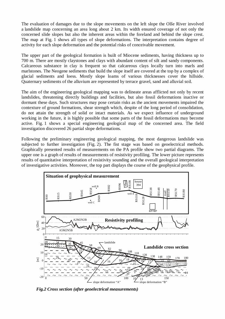
The evaluation of damages due to the slope movements on the left slope the Olše River involved a landslide map concerning an area long about 2 km. Its width ensured coverage of not only the concerned slide slopes but also the inherent areas within the foreland and behind the slope crest. The map at Fig. 1 shows all types of slope deformations. The interpretation contains degree of activity for each slope deformation and the potential risks of conceivable movement. The upper part of the geological formation is built of Miocene sediments, having thickness up to 700 m. There are mostly claystones and clays with abundant content of silt and sandy components. Calcareous substance in clay is frequent so that calcareous clays locally turn into marls and marlstones. The Neogene sediments that build the slope itself are covered at the top by a complex of glacial sediments and loess. Mostly slope loams of various thicknesses cover the hillside. Quaternary sediments of the alluvium are represented by terrace gravel, sand and alluvial soil. The aim of the engineering geological mapping was to delineate areas afflicted not only by recent landslides, threatening directly buildings and facilities, but also fossil deformations inactive or dormant these days. Such structures may pose certain risks as the ancient movements impaired the contexture of ground formations, shear strength which, despite of the long period of consolidation, do not attain the strength of solid or intact materials. As we expect influence of underground working in the future, it is highly possible that some parts of the fossil deformations may become active. Fig. 1 shows a special engineering geological map of the concerned area. The field investigation discovered 26 partial slope deformations. Following the preliminary engineering geological mapping, the most dangerous landslide was subjected to further investigation (Fig. 2). The fist stage was based on geoelectrical methods. Graphically presented results of measurements on the PA profile show two partial diagrams. The upper one is a graph of results of measurements of resistivity profiling. The lower picture represents results of quantitative interpretation of resistivity sounding and the overall geological interpretation of investigative activities. Moreover, the top part displays the course of the geophysical profile.

0 50 100 150-20

-10

0

10

20

[m]

0 15 3045

5869 82 96 108 118 128 138 148 159 170 180

2833

3419

3116 28

2314

1815 27 20

1726

16

36

23

29

17

68

2248

60

130 50 35

16

2929

2729

2521 20

30

10 13

9 10 16 mΩ 13 24

1326

16 16 16 18

22

18

O

O

O O

O

O

O

O

O

O

O

O O

OO

O

O

O

O

O O

O O

O

O O

O

O O

O

O

O

O OO OOO

O

O

OO

O O

O

OO

O

OO O

OO

O

OO

O

OOO O

OO

OO O

O

O

O

O OO

O

O

OO O

O

δδδ

δδδδ

δδ

δ

δδδδδ

δδ

δ

δ

δ

δδ

δδδ

δδ

δδ

δδδ

δ

landslide

slope deformation “A” slope deformation “B”

Fig.2 Cross section (after geoelectrical measurements)

Landslide cross section

Situation of geophysical measurement

well A

well B

well C

roa

d

garage

she

d house 394

RS

0

RS

15

RS

30

RS

45

RS

58

RS

69

RS

82

RS

96

RS

108

RS

118

RS

12

8 RS

138

RS

148

RS

15

9

RS

17

0

RS

18

0

Resistivity profilingA2M2N2B

A5M2N5B0

20

40

60

a ρ Ω[

m]

After the primary geophysical interpretation we made a physical model of the slope. The further step – geological interpretation – was based on general geological principles along with our geological understanding of the region. The profile was subdivided to eight physical units characterized lithologically or geodynamically. Then the physical model of the slope was examined in more detail. The complex of geophysical methods was extended by shallow refraction seismic, seismic tomography, and logging survey. Besides these methods, we installed boreholes for standard documentation of drilling core and logging. The boreholes were consequently used as monitoring holes and as boreholes for precise inclinometer survey. The logging results in one hole are given in Fig 3. The methods used: gamma log, gamma gamma log, neutron neutron log, resistivity log with normal device (Rap 0.11, Rap 0.41), calliper log, photometry, thermometry, and sonic logging. A standard task of logging is to specify the lithological profile. The base of Quaternary cover was detected at a depth of 5 m. Neogene sediments, described geologically as claystones with capsules of fine sand up to 5 cm or sandy limestone, were indicated by gamma log and neutron neutron log as claystone and sandy claystone, indicating the total strata thickness up to 2 meters or more.

The curves of gamma gamma log and sonic log characterize two blocks of different physical properties and one anomaly defined by depth. The first block reaches to a depth of about 5.3 meters. It mostly coincides lithologically with Quaternary sediments, including by the top layer of weathered Neogene claystone. The lower block is built up from Neogene sediments and it contains the anomaly. According the features of physical properties, we can say that the physical properties become better with depth. Therefore, according to the geophysical survey, the slipping plane can be expected anywhere within this layer; thus the logging survey is not capable to delineate the location where the slipping plane could be expected. Such statement is very important for the geotechnical engineer who makes appropriate stability solution. The check measurements of the precise inclinometry confirmed movement in this borehole at a depth of 5.1 m in the spring of 2001 (Novosad L., 2001). These findings are consistent with the results of the logging survey, and are not against the statements deduced from the distribution of physical properties around the hole. The anomaly characterized by the changed physical properties occurs from 7.0 m to 7.7 m. The biggest deviation from the normal field is obvious on the curves of density logging and the arrival time of ultrasonic wave to the first sensor. Another deterioration can also be found on the curve of attenuation. All these changes of physical parameters of the layer indicate that the layer can be described as a layer of plastic clays. According to this characteristic we can establish a hypothesis

Fig.3 Well logging on landslide

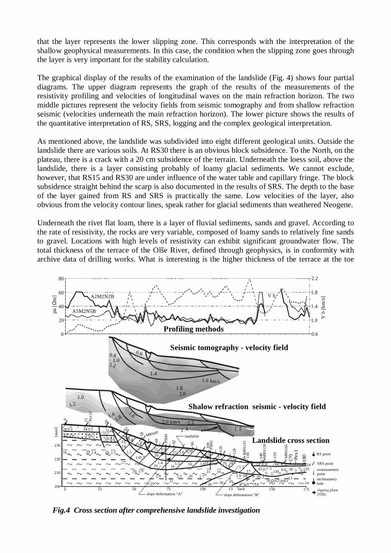
that the layer represents the lower slipping zone. This corresponds with the interpretation of the shallow geophysical measurements. In this case, the condition when the slipping zone goes through the layer is very important for the stability calculation. The graphical display of the results of the examination of the landslide (Fig. 4) shows four partial diagrams. The upper diagram represents the graph of the results of the measurements of the resistivity profiling and velocities of longitudinal waves on the main refraction horizon. The two middle pictures represent the velocity fields from seismic tomography and from shallow refraction seismic (velocities underneath the main refraction horizon). The lower picture shows the results of the quantitative interpretation of RS, SRS, logging and the complex geological interpretation. As mentioned above, the landslide was subdivided into eight different geological units. Outside the landslide there are various soils. At RS30 there is an obvious block subsidence. To the North, on the plateau, there is a crack with a 20 cm subsidence of the terrain. Underneath the loess soil, above the landslide, there is a layer consisting probably of loamy glacial sediments. We cannot exclude, however, that RS15 and RS30 are under influence of the water table and capillary fringe. The block subsidence straight behind the scarp is also documented in the results of SRS. The depth to the base of the layer gained from RS and SRS is practically the same. Low velocities of the layer, also obvious from the velocity contour lines, speak rather for glacial sediments than weathered Neogene. Underneath the rivet flat loam, there is a layer of fluvial sediments, sands and gravel. According to the rate of resistivity, the rocks are very variable, composed of loamy sands to relatively fine sands to gravel. Locations with high levels of resistivity can exhibit significant groundwater flow. The total thickness of the terrace of the Olše River, defined through geophysics, is in conformity with archive data of drilling works. What is interesting is the higher thickness of the terrace at the toe

1.6 km/s

1.0

1.4

0.60.8

1.2

1.82.0

Seismic tomography - velocity field

1.0

1.2

1.41.8

1.62.0 km/s 2.2

2.4 1.8

Shalow refraction seismic - velocity field

0 25 50 75 100 150 175

0 15

30

45

58

69 82 96

108

118

128

138

148 15

9

170

180

28

33

34

1931

16 282314 18

1527

20

2017

26

16

36

23

29

1768

2245

6050

2435

16 29 29

27

29

2521

30

22

139 10

16 mΩ13

24

1326

16 1616 18 18

O

O

OO

O

O

δ

δ δδδ

δ

200

210

220

230

[mas

l]

Pe

x1

Pex

15

MRS60

MR

S13

5

MR

S15

0

MR

S1

65

PIM

4

PIM

2

0.5

0.4

3 km/s

0.5

2.3

0.71.7

2.9

1.8

0.5

1.6

2.72.2

1.5

1.00.6

1.4

2.92.9

0.7

0.40.6

1.52.5

0.6

0.40.5

0.7

2.4

1.0

0.5

O

130 0.6

fault

landslide

slope deformation “A” slope deformation “B”

SRS point

extensometricpoint

RS point

inclinometryhole

Landslide cross section

Profiling methods0.6

1.0

1.4

1.8

2.2

V b

[km

/s]V b

0

20

40

60

80

ρΩ

a [

m] A2M2N2B

A5M2N5B

Fig.4 Cross section after comprehensive landslide investigation

of the slope. It could be caused by powerful erosive activity of Olše River within the postglacial period or by small strength of the bedrock. This may be given by tectonic deterioration of Neogene claystones (Fig. 4). The most geodynamically active structure is a shallow slope deformation – landslide. In the picture it is marked by thick hatch. The landslide material consists of a mixture of all types of Quaternary sediments and the bedrock material – Neogene clays. All sediments are kneaded and they physically form one layer. In the longitudinal direction, from geophysical measurements, we can appoint two partial landslides. From curves of the resistivity profiling and from the seismic measurements, it is clear that the rock massif is in the subsurface under tensilly strain from the slope edge to SRS75. According to the seismic tomography, the active landslide is quite released, especially at the top. Up to 70 m from the face edge, the rates of longitudinal waves drop below 0.6 km/s, which is the evidence of their low bulk density and extensive mechanical disturbances. Underneath the shallow landslide we can encounter two other storeys of slope failure by a deep slope deformation. With regard to an expressive minimum of velocities near 50 m stationing, it is obvious that there is significant tension zone. We can deduce that the central storey of the slope deformation is in active, nevertheless slight, movement. Only the lower storey is considered as a steady structure. The central and lower storeys are marked by sparse hatch. The central storey of the slope deformation cannot be distinguished within the profile by resistance (RS82, 96, 108). The bottom of the second storey was detectable both by seismic measurements and logging. The lower slipping plane was detected geoelectrically, and within the lower part of the landslide also by the method SRS and logging curves. Tension disturbances of deep deformations near the slope toe are visible not only in the field of velocities but also on the quantitatively determined low rates on SRS60, where, from interpretation of critical distances, the velocity is 0.7 km/s up to the depth of about 17 m. In the field of velocities from the seismic tomography results we see interesting distribution of velocities. In the upper part of the landslide, with 70 meters spacing, we can find low velocities of longitudinal waves. Within the central storey of the landslide the velocities drop below 0.8 km/s; the low storey shows maximum velocities reaching 1.2 km/s. Such low velocities at depths up to 15 meters are utmost anomalous, confirming significant tension stress of all storeys of the slope deformation. On contrary, the lower part of the slope exercises growth of velocities up to 1.6 km/s. The velocity contour lines show inversion in the section of 80 – 100 meters. The anomaly of the increased velocities occurs at the central slipping plane. The increased velocities can result from higher rock stress through friction on the slipping plane or by compaction of material within the central and low storeys of the slope deformation. The changes in velocities from the seismic tomography correspond with the logging results. We can assume possible explanation that the decline in velocities is not caused only by disturbances of rocks but it is also given by transition from the range of increased strains into the range of normal strains. There is a discrepancy between the velocities gained from the seismic tomography and the shallow refraction seismic survey. The values from the plus-minus method are higher than allowable inaccuracy of measurement or errors. The explanation must be based on the principles of the methods. The penetration method deals mostly with rays parallel to the earth surface. On contrary, velocities by seismic tomography represent the average value of velocities in all directions. Therefore, if Fig. 4 shows higher values gained from the transmission method, we must seek for the reason why the velocity is higher in this direction. The only explanation is the horizontal tension. If the ration of the velocities is less than 0.8, the horizontal velocities are higher by 1.5* then the vertical velocities. Here, we must repeat that the seismic measurements examine conditions that cannot be resolved by conventional engineering geological investigation. The stability calculations must be expanded by a variable of horizontal tension.

In the post glacial period, the Olše River eroded down to the current altitude of the recent terrace, which resulted in undercutting of the slope and formation of slope deformation “B”. Due to the landslide, the river was forced away from the slope toe. Further erosion gradually denuded the material of the slope deformation and the slope toe got loose again. A new slope movement gave rise to slope deformation “A”. The materials of the deep deformations (Neogene clays) are disturbed in two ways. After deglaciation, the top layer of clays was relieved and subhorizontal fractures evolved. When the side erosion and the first slope movement got close, the clays were horizontally transformed with evolution of vertical fractures. These processes led to increase in water content in the clays, which, together with the failure caused by slope movement, resulted in decrease of the resistivities of the deep deformations. These were also enhanced by loosening of the sand formations, which consequently play a role of water influent beneath the slope deformation or straight to the slipping planes. Therefore, the resistivities of the deep deformations are lower than the resistivities of the shallow landslides where the landslide material is more disturbed. The increased resistivities of the shallow slope deformations are also due to inclusions of glacial sandy sediments, as well as air fissures. Similarly, the resistivities of the deep landslides are lower than the resistivities of the relatively less disturbed clays of the underlying bedrock. And there are not vertical fractures or failure by slope movement. The bedrock of the mentioned geological complexes is built up from Neogene sediments. The lowest resistivities can be detected at the slope toe on RS118 and RS148. It is highly probable that these Neogene sediments are tectonically weakened here. This is the reason why the side erosion advanced so far. Near the zone of weakness there is a zone with higher resistivities. Our assumption is that the layer consists of more compact sediments than Miocene claystones. It could be a sandy formation or a formation bearing more calcareous compartments. According to the results of tomography we can consider the decline in velocities at lower depths for the 70 meter stationing. The drop in velocities is also recorded on the logging curves. It is probably caused by failure of Neogene sediments in the bedrock of the landslide. That supports the assumption that the origin of the slope deformation in this place is bound to this failure of the Neogene claystones.

The information gained from the investigation and monitoring (groundwater monitoring and inclinometry) at the site was used in stability calculations. The inclinometer measurements confirmed as the most active shallow slipping plane (circular in the upper part, slightly undulate at the bottom). Therefore, the slope stability was evaluated by calculation of safety factors - against movement along this slipping plane considered in the calculation as broken.

Our own program STABLOM2 made the calculation, the Pettersson’s and Bishop’s methods adjusted for calculation of the safety factors along irregular slipping plane. The slope geometry is shown in Fig. 5. The shape of the slipping plane was defined in the former investigation. We also determined the safety factor along circular slipping plane: value s = 0.96 (according to the results of reverse calculation along slipping plane for the lower part of the slope with the safety factor = 1, characterizing the indifferent state of equilibrium). New calculations have introduced parameters of shear strength, established by the previous reverse calculation as a weighted average of parameters of the materials through which the mentioned slipping plane runs. A series of calculations was

initiated by determination of the safety factor along the broken slipping plane, under the condition of water table in 2000 year (it was used in calculations under the last investigation). Afterwards, the calculation for the decreased level of the water table that was characteristic for the situation before starting our stabilization activities (installation

of drainage holes) was done. The last calculation simulated the situation after stabilization (significant fall of the water table). The calculated safety factors for the landslide movement along the defined slipping plane are given in the following table:

Level of water table

Depth to water table below terrain surface [m] Safety factor

HV1 HV3 slope edge 10 m behind slope edge

Initial - in 2000 3,64 3,60 5,63 6,20 1,11 Before dewatering 2,50 1,00 3,50 3,50 1,00 After dewatering 4,60 5,20 7,50 6,50 1,27

From the table, it as clear that the calculated values of the safety factors are highly dependent on the altitude of the water table. For a consideration of the stability calculations and confirmed monitoring we decided in the first step to stabilize the landslide through dewatering. This was carried out step-by-step: installation of long horizontal drainage holes, construction of surface drainage, installation of short horizontal drainage holes, and revival of dewatering of the house on the landslide (Fig. 6).

The long horizontal drainage holes were drilled from the front face of the landslide with a drilling set, by navigated drilling (both direction and inclination) along the shallow slipping plane. After 95 m, the holes were brought out on the surface in a plain above the landslide. The horizontal drainage hole HOV2 was132 meters long, and HOV3 135 m. The holes were not driven in straight lines; they were deflected to avoid the base of the house. The surface drainage, made of prefabricated troughs, had a shape of a horseshoe in the upper part of the landslide. From the upper part of the horseshoe there were installed the upper short horizontal drainage holes in order to dewater the plain above the landslide. The drilling technology was the same as for the long holes. The lengths are: 51 m for HOV5 and 54 m for HOV4, drilling angle was 10° above horizontal. The

30 m

0

N

O

OOOO O O

OOO

O O O

δ δδ δ

δ

[ma

sl]

2 14567

891011

12

1314

3

15

PIM

4

PIM

2

drainage hole projection

primary water table

HP5

220

2000 50 100 150

Cross section

HP3 PI

M4

PIM

2

HP1

1

2

34

56

78

910

11

1213

1415

GB

6

GB

4G

B2

GB

5

GB

4G

B2

GB

3G

B1

St10

St12

HO

V1

HO

V5

HO

V3

HO

V4

HO

V2

water inflow

to

drainage hole

235

230

active landslide

scarp

erosive groove

10

PIM2

extenzometry point

hole for precise inclinometry

GB6 point of geodetic measurement

St10 well

HP1 hydrogeological hole

projection of drainage hole

Fig. 6 Landslide stabilization

Landslide map

purpose of the short horizontal holes (45 m long) in the lower part of the landslide was to dewater the hole occurring in the lower accumulation part of the slope deformation. All of the horizontal drainage holes were checked with a television camera, which gave us a detailed knowledge on their functioning and condition of perforation of polyethylene pipes. The television inspection revealed more complicated water circulation in the massif than supposed in general. The alternation of spots with water inflow to the hole and dry spots also occurs in half a meter intervals, in extreme conditions more frequently. There are no positions where the water does not come to the hole within the interval of five meters. At the holes we can distinguish intervals where water run down heavily or slightly along the casing, intervals where water ran along the casing under the higher level of groundwater, and intervals with no water at all. Fig. 7 represents typical video documentation from horizontal drainage holes. Shot C: 5-mm perforation slots in the casing of the drainage hole (8) and a camera light rod (6). Shot B: an interval with slight inflow of water, water coming from the landslide along the bottom of the casing (2) and intervals of occasional draining of water to the hole (1). These parts are covered by limonite. Other perforation slots (5) show heavier and active inflow of water at the time of our inspection. These intervals typically behave as a source of intensive reflection. Shot E, F: the best TV documentation of horizontal drainage holes. E: water running from the upper perforation. F: water flowing from a hole at the bottom of the casing in foreground, and water running from a hole at the top of the casing in background.

If we plot the intervals of intensive water inflows to drainage holes, they will fall on one line, where the biggest deformations of the landslide were detected (see Fig. 6). We cannot exclude a hypothesis that the sand excavated during installation of the monitoring hole is not a residue of the old slope deformation “B”. The essential part of the landslide monitoring before, during, and after the stabilization is observing of the groundwater regime. For this landslide we monitored the water table at three holes and the outflow from four horizontal drainage holes. The level of the water table across the landslide is measured at the HP1 and HP3 holes from the beginning of the monitoring. At the beginning of the stabilization, the HP5 hole was installed on the plain above the landslide and then included into the monitoring system. At first, the water level was measured once a week; afterwards, from the beginning of the stabilization, it was measured on a daily basis. The results are shown in Fig. 8.

68

Shot C

4 7

9

Shot F

1

2

5Shot B

7

Shot E

1

5

6

9

8

2

4

7

trace of occasional inflow

water flowing on of hole bottom

water springing from hole bottom

trace of gravitating water

rod of lighting

water springing from perforation

perforation (diametr 5 mm)

pulling cord

Fig. 7 TV logging of outflow from drainage hole

Moving way of videocamera:

- shot F: camera pulled on cord- shot B, C a, E: camera pushed by rod

Type of hole inside:

- shot C: without inflow- shot B: weak inflow- shot E, F: strong inflow

From the picture, it is obvious that before the beginning of dewatering the landslide the water table fluctuated significantly. Fluctuations reached 1.5 m and 2.5 m at HP1 and HP3, respectively. The picture shows data from two rainfall metering stations. Certain rain brought about nearly immediate increase of the water table; some were almost without any impact (9.4.2001). The rain of the season around April 22nd produced increase of the water table, resulting in the landslide movement (as we know from inclinometry and extensometry). Similar situation repeats around July 18th. The increase of the water table was more profound at HP3 hole, where, in the tension zone of the landslide, the water percolation was easier and surface water came from the plain above the landslide. The importance of the drainage holes in respect of the water level in the massif is clear from the rapid decrease of the water table after the beginning of the drainage activities. The decrease was 5 m, 3 m, and 4 m at HP3, HP1, and HP5 hole, respectively. It is important that water table did not reach the original altitude any more. Moreover, the increment over the rain season is lower then before. Thus, the massif is under lower stress by the high levels of the water table, also the dynamic stress from groundwater fluctuation is decreased. The 2001/2002 winter monitoring another decrease of the water table was watched. At the end of January 2002, during the thaw season, the water table slightly went up; nevertheless, it did not reach the level measured in the rainy season of August 2001. The time period when the landslide was exposed to higher levels of the water table was shorter than in August 2001. The daily monitoring of the water table shows that some events of rapid increase in water table happened at the HP3 hole, and occasionally also at HP5 hole. Moreover, for certain rapid changes we subsequently discovered typical gradient curves, which explains these anomalies. The system of the underground percolation in the landslide and its vicinity is very complicated, consisting of several interrelated subsystems. The monitoring of the water level and the landslide proves benefits from dewatering resulting in decreased stresses in the massif and its vicinity. In late January and early February of 2002, after another thaw season, the landslide body was saturated with water. Its dewatering will probably take certain time. The further water decreasing was noted in the second part of 2003. According our knowledge this effect was caused with the mining activity. Since October 2001, when the hydrogeological holes were completed, we have also monitored the quantity of the water outflow. In Fig. 8, the outflow rates are marked in the graph of water level fluctuation. It is obvious that the fluctuations have the same character like the fluctuations of the

hole HG1

hole HG3

hole HG5

200320022001

rainfall at station Karvina

outflow

landslide drainage starting

wa

ter

tab

le [

m]

tota

l ou

tflow

[l/s

]ra

infa

ll [m

m/d

ay]

Fig. 8 Water table and outflow changes9

8

7

6

5

4

3

2

1

0

20

40

60

80

0

0.1

0.2

0.3

water table at the respective holes. Little discrepancies are provided for certain inaccuracy in measurement. During the thaw season the outflow increased from 0.1 l/s to 0.2 l/s. Then the outflow fell rapidly. The recent quantities are about 0.04 l/s. The highest outflow is from HOV2 (the southern part of the landslide). According to the owner of the house, considerable surface deformations were recently observed in this part of the landslide. In late January, after the thaw season, the outflow was also increased at the short hydrogeological holes installed within the tension zone of the landslide. The holes meet the target as they take off the water from the massif above the landslide and from the tension zone of the landslide, enhancing the slope stability. Another important component of the monitoring technique during observation of the slope deformations is inclinometry. Measurements were conducted in two holes (see Map, Fig. 1, and Fig. 4 – cross section). Results are given in Fig. 9. The inclinometry measurements indicated movements in two periods: between April 27Th and May 9th, and between July

19th and August 15th of 2001 (before launching the stabilization). Movement was recorded at both holes. At the upper PIM4 hole we detected a spring deformation of 60 mm at a depth of 6 m. The

lower hole revealed 30 mm deformation at a depth of 5 m. The size of these movements complies with the extensometry measurements. Another movement in the summer was not so distinctive. It reached 10 mm, which is confirmed by zone extensometer measurements. Very important observation is the backward move of the PIM2 mouth after August 15th (immediately after boring the horizontal drainage hole). This is not a movement along a narrow slipping plane but the entire hole becomes slant against the slope. Comparing the curves, it is clear that the biggest backward movement happened between September 15th and 19th. Gradual fading of the movements was also detectable at the PIM4 hole. The amplitude at each hole is individual. At PIM2 hole in the centre of the landslide the size of the backward move is approximately 9 mm, at PIM4 hole near the scarp it is 2.5 mm. As mentioned above, the extensometry measurements describe similar behaviour of the dewatered slope.

Fig. 9 Precise inclinometry results (modified by Novosad 2003)

0 20 40

dep

th [m

]de

pth

[m]

29. 1.200127. 4.200115. 8.200120.11.2003

vect

or c

ompo

nent

alo

ng fa

ll lin

e

vect

or c

ompo

nent

alo

ng c

onto

ur li

ne

-20 0 20

12

6

0

30

24

18

12

6

0PIM2

PIM4

[mm]

t [day]0 100 200 300 400 500

t [day]0 100 200 300 400 500

t [day]0 100 200 300 400 500

mo

vem

en

t [m

m]

-80

-60

-40

-20

0

20

40

mov

em

ent

[mm

]

-80

-60

-40

-20

0

20

40

mo

vem

en

t [m

m]

-80

-60

-40

-20

0

20

40

mov

em

ent

[mm

]

-80

-60

-40

-20

0

20

40

9.11

.200

0

9.11

.200

0

23.1

.200

1

23.1

.200

1

21.3

.200

1

21.3

.200

1

10.5

.200

2

10.5

.200

2

14.6

.200

1

14.6

.200

1

18.7

.200

1

18.7

.200

1

21.8

.200

1

21.8

.200

1

10.1

0.20

01

10.1

0.20

01

4.12

.200

1

4.12

.200

1

22.1

.200

2

22.1

.200

2

26.3

.200

2

26.3

.200

2

28.

1.2

001

29

.3.2

001

27.4

.20

01

1.8

.20

01

12

.11.

200

1

27.4

.20

02

19

.7.2

001

mov

em

ent

alo

ng fa

ll lin

e [m

m]

Fig. 10 Extenzometry results

1-2

2-3

3-4

5-6

6-7

7-8

8-9

9-10

10-11

11-12

12-13

13-14

14-15

4-5

landslide stabilization moment

landslide stabilization moment

0

20

40

60

Movementof inclinometricalhole mouth

Extenzometrical movements

Another important component of the landslide monitoring is the tape extensometry. The example (Fig. 10) is from the Ujala landslide. Fig. 6 shows the layout of the extensometer posts. The extensometer points are mapped into the geological section (Fig. 4) The results of the extensometry measurements are in Fig. 10. There are obvious two dislocations. The first is a landslide movement detected on 10 May. The most important movement occurred between the points E12-E13, E11-E12, E7-E8, and E5-E6. At E12-E13 we detected extension of the distance by about 70 mm. The extension gradually equalled between E11-E12 (20 mm), E7-E8 (20 mm). Between E6-E7 the distance extended by 10 mm. The contraction between E5 and E6 compensates the extension in the other part of the slope. After indication of the important movement of the slope, we involved a stage of activities of observing the end of the movement. Another movement happened in the summer following heavy rains. This movement was slighter; 10 mm deformation was found between E12 and E13. The extension was compensated between E7 and E8. Also this movement is classified from view of time as incidental; it was not identified in further measurements. The measurements carried out after the landslide stabilization confirms that there are no new movements within the slope deformation. The changes in distances between the points E3-E4 and E2-E3 have been currently progressing gradually, which means downward move of E3 within the road bank. The detailed study of the changes in the distances E7-E8 and E8-E9 has proved slight changes in these distances since August 2001. Point E8 has moved against the slope, according to extensometer measurements by about 5 mm. Points E4 to E9 have the same tendency. This effect is due to the slope dewatering as the backward movement started in August 2001. The changes fully correspond to the inclinometer measurements. After comparison of the results of both measurement techniques, we plotted time changes of the movement of the hole mouths of the inclinometry holes (Fig.10). Comparison with the results of the zone extensometry brings the same conclusion. In this paper I would like to show a system of the research of slope deformation and the research results in a case landslide study. These are the results of the landslide stabilization Pod Ujalou I. The landslide was stabilised by dewatering, respectively by both subsurface and surface dewatering. The subsurface dewatering was carried out through five horizontal drainage holes, installed using new technology – navigated drilling. The surface dewatering system consists of two elements. Troughs trapping run off water from the scarp of the landslide lead to checking shafts at he side of the landslide. Then the water runs through plastic hosepipes outside the landslide. The slope deformation was observed using six independent methods: inclinometry, extensometry, levelling, measurements of water table and outflow from hydrogeological holes, geodetical survey, acoustic and electromagnetic emissions, and visual inspection. The monitoring results confirm the effect of the landslide dewatering. What is important is the increase of the water table, both in the landslide and its vicinity. According to the stability calculations, the dewatering results in stability improvement at the edge of the long-time stability; therefore, the landslide will require further monitoring. The fall in water table results in the increase of the stability coefficient by 27 % to 1.27. We expected that the significant drop of the water table would exercise an effect on volume changes of soils. Certain special changes in behaviour of the massif were observable in the precise inclinometry and extensometry measurements.

Reference: Bláha P. 1993. Geofyzikální metody při průzkumu svahových deformací (in Czech). Praha,

Geofond (in Czech). Bláha P. a kol.: Doubrava, závěrečná zpráva, mapování sesuvů a geofyzika., Geotest Brno., 5/2000,

unpubl (in Czech). Bláha P. a kol.: Doubrava, Pod Ujalou I - doprůzkum., Geotest Brno., 12/2000, unpubl (in Czech). Bláha P. a kol.: Doubrava, Pod Ujalou I - monitoring 2000., Geotest Brno., 12/2000, unpubl (in

Czech). Bláha P. a kol.: Doubrava, Pod Ujalou I - monitoring 2001., Geotest Brno., 12/2001, unpubl (in

Czech). Bláha P. a kol.: Doubrava, Pod Ujalou I - monitoring 2002., Geotest Brno., 12/2002, unpubl (in

Czech). Diedda G. P. et al 1996 An application a combined refraction – reflection seismic method to s

landslide study, 2nd Meeting Environmental and Engineering Geophysics, Nantes, EEGS, p. 117-120.

ISRM Suggest Methods for Monitoring Rock Movements Using Inclinometrers and Tiltmeters., Rock Mechanics, 10, 1977, s. 81 - 106.

Kelly W. E. & Mareš S. (eds) 1993. Applied geophysics in hydrogeological and engineering practice. Amsterdam, Elsevier.

Kovari K.: Methods of monitoring landslides., General report, Landlides, Balkema, Rotterdam, 1988.

Lukeš J. 2000. Zpráva o karotážním měření ve vrtech PIM 2 a PIM4. Praha, Auatest, unpub (in Czech)l.

Novosad L.: Výsledky měření přesné inklinometrie na lokalitě Ujala I - monitoring, 13. opakované měření dne 2.12.2001 ve vrtech PIM2 a PIM4., G4C, Praha, 2001, unpubl (in Czech).

Novosad L.: Výsledky měření přesné inklinometrie na lokalitě Ujala I - monitoring, ve vrtech PIM2 a PIM4., G4C, Praha, 2002, unpubl (in Czech).