Large Bets and Stock Market Crashes Albert S. Kyle Robert H. Smith School of Business University of Maryland [email protected]Anna A. Obizhaeva Robert H. Smith School of Business University of Maryland [email protected]July 31, 2012 Abstract We use market microstructure invariance, as developed by Kyle and Obizhaeva (2011a), to examine the price impact and frequency of large stock market sales documented for the following five stock market crash events: the stock market crash late of October 1929; the stock market crash of October 19, 1987; the sales of George Soros on October 22, 1987; the liquidation of J´ erˆ ome Kerviel’s rogue trades by Soci´ et´ e G´ en´ erale in January 2008; and the flash crash of May 6, 2010. Actual price declines are similar in magnitude to declines pre- dicted based on parameters estimated from portfolio transitions data by Kyle and Obizhaeva (2011b). The two flash crash events had larger price declines than predicted, with immediate rapid V-shape recover- ies. The slower moving 1929 crash had smaller price declines than predicted. Reconciling the predicted frequency of crashes to observed frequencies requires the distribution of quantities sold either to have fatter tails than a log-normal or a larger variance than estimated from portfolio transitions data. Using data available to market participants before these crash events, microstructure invariance leads to reason- able predictions of the impact of these systemic crash events.
We use market microstructure invariance, as developed by Kyleand Obizhaeva (2011a), to examine the price impact and frequencyof large stock market sales documented for the following five stockmarket crash events: the stock market crash late of October 1929;the stock market crash of October 19, 1987; the sales of George Soroson October 22, 1987; the liquidation of Jerome Kerviel’s rogue tradesby Societe Generale in January 2008; and the flash crash of May 6,2010. Actual price declines are similar in magnitude to declines pre-dicted based on parameters estimated from portfolio transitions databy Kyle and Obizhaeva (2011b). The two flash crash events had largerprice declines than predicted, with immediate rapid V-shape recover-ies. The slower moving 1929 crash had smaller price declines thanpredicted. Reconciling the predicted frequency of crashes to observedfrequencies requires the distribution of quantities sold either to havefatter tails than a log-normal or a larger variance than estimated fromportfolio transitions data. Using data available to market participantsbefore these crash events, microstructure invariance leads to reason-able predictions of the impact of these systemic crash events.
Introduction
Once in a while, stock markets plummet and rattle financial markets, leavingstunned market participants, puzzled economists, and frustrated policymak-ers unable to explain why the crash or panic they just witnessed happenedat all. In the aftermath of crashes and panics, it has typically emerged thatspecific market participants were engaged in heavy selling as market disloca-tions unfolded. This paper studies the following five stock market crashes,for which data on the magnitude of selling pressure became publicly availablefollowing official studies of the crashes:
• After the stock market crash of October 1929, it was documented thatmargin calls resulted in massive selling of stocks and reductions in loansto finance margin purchases.
• After the October 1987 stock market crash, the Brady Commission re-port (1988) documented the quantities of stock index futures contractsand baskets of stocks sold by portfolio insurers.
• After the futures market dropped by 20% at the open of trading threedays after the 1987 crash, it was revealed that George Soros had exe-cuted a large sell order during the opening minutes and later sued hisbroker for an excessively expensive order execution.
• After the Fed cut interest rates by 75 basis points in response to amarket plunge on January 21, 2008, it emerged that, around the sametime, Societe Generale liquidated billions of Euros in stock index futurepositions accumulated by rogue trader Jerome Kerviel.
• After the flash crash of May 6, 2010, a joint study by the CFTC andSEC identified approximately $4 billion in sales of futures contracts byone entity as a trigger for the event.
Before the first two of these events—the crashes of 1929 and 1987—thesize of potential selling pressure was widely known and publicly discussed,but market participants had different opinions concerning whether the sellingpressure would have a significant effect on prices. Before the last three crashevents—associated with the Soros trades, the Societe Generale trades, andthe flash crash trades—the sellers knew precisely the quantities they intendedto sell, but they either estimated inaccurately or were willing to incur the
1
much lower prices they received compared to prices before the trades weremade.
The purpose of this paper is to examine these five crash events fromthe perspective of market microstructure invariance, a conceptual frameworkdeveloped by Kyle and Obizhaeva (2011a). Our main result is that, giventhe information about the dollar magnitudes of potential selling pressurewhich existed before these crashes occurred, market microstructure invari-ance would have made it possible to generate reasonable predictions of thesize of the future declines. Our results suggest that market microstructureinvariance can be used as a practical tool to help quantify the systemic riskswhich result from sudden liquidations of speculative positions.
Two features of market microstructure invariance make practical predic-tions possible.
First, the invariance principle, by its very nature, implies that only asmall number of parameter values need to be estimated, and these parame-ter values are the same for active markets and inactive markets, liquidationsof large positions and liquidations of small positions. Thus, rather thanattempting the statistically impractical task of estimating ad hoc “marketcrash” paramenters from a historical database, including a presumably smallnumber of rare crash events for specific markets, a small number of necessaryparameters can be estimated from databases pooling a large number of typ-ical transactions in many different markets, some active and some inactive.In this paper, we use the parameter estimates Kyle and Obizhaeva (2011b)obtain from a database of more than 400,000 portfolio transition trades inindividual stocks, typically executed on different days and under normal mar-ket conditions. In a portfolio transition, a third-party “transition manager”executes trades which convert a legacy institutional portfolio managed byan incumbent asset manager into a target portfolio managed by a new assetmanager. Portfolio transition trades are well-suited for estimating the sizeand price impact of institutional trades because the sizes of the trades to beexecuted are objectively known in advance and are typical in size to otherinstitutional trades.
Second, given parameter estimates, practical application of microstruc-ture invariance requires limited market-specific data. To estimate the marketimpact of a given dollar amount of selling pressure, the only additional piecesof information required are estimates of expected dollar volume and expectedreturns volatility, both of which can be obtained from recent historical data,such as daily returns and dollar volume data for previous months. It is not
2
necessary to have additional types of information, such as the extent of ordershredding or other characteristics of traders.
In a speculative market, price fluctuations occur as a result of some in-vestors placing “bets” which move prices, while other traders attempt toprofit by intermediating among the bets being placed. A bet is an “intendedorder” whose size is known in advance of trading. The speed of trading variesacross markets, i.e., “business time” passes more quickly in active marketsthan in inactive markets. Market microstructure invariance is based on theintuition that when appropriate adjustment is made for the rate at whichbusiness time passes, market properties related to the dollar rate at whichmark-to-market gains and losses are generated do not vary across markets.As discussed in more detail below, this implies that, appropriately adjustedfor market speed in a specific manner related to dollar volume and volatility,the size distribution of bets and the price impact of bets do not vary acrossmarkets.
Large bets can result either from trading by one large entity or from cor-related trades of multiple entities based on the same underlying motivation.Societe Generale’s liquidation of Kerviel’s rogue trades, George Soros’s largeorder to sell futures contracts, and the $4 billion sale during the flash crashare three examples of bets placed by one entity. In all three cases, the sellersintended to trade specific quantities before the trades were executed. Theforced margin sales by numerous market participants during the 1929 crashand the correlated sales by investors following the strategy of portfolio insur-ance during the October 1987 crash are two examples of bets representingcorrelated trades by multiple traders acting for the same underlying reason.
In contrast to bets, the intermediation trades which take the other sideof bets are not the result of intentions to buy specific quantities formulatedin advance of the trading opportunities presenting themselves. For example,many of the traders who purchased futures contracts as prices plummetedduring the flash crash of May 6, 2010, were probably responding to the unex-pected opportunity to turn a quick profit by making purchases at attractiveprices, not carrying out specific purchase plans formulated before the flashcrash occurred.
Using dollar volume and returns volatility as its only inputs in addition toa single market depth parameter estimated from portfolio transitions data,the invariance hypothesis generates predictions about the size of the priceimpacts resulting from the innovations in order flows documented for thesecrash events. Table 1 summarizes our results, using volume and volatility
3
estimated from daily data over the month before the crash event. For each ofthe five crash events, the table gives the estimated size of the dollar amountsliquidated (percent of daily volume), actual price decline (percent), predictedprice decline (percent), and predicted frequency of occurrence of such largebets.
Table 1: Summary of Five Crash Events: Actual and Predicted Price Declines
Actual Predicted %ADV %GDP Frequency
1929 Market Crash 24% 49.22% 241.52% 1.136% once in 5,539 years1987 Market Crash 32%-40% 19.12% 66.84% 0.280% once in 716 years1987 Soros’s Trades 22% 7.21%—15.83% 2.29% 0.007% once per month2008 SocGen Trades
STOXX 10.50% 13.82% 54.36% 0.283% once in 895 yearsDAX 11.91% 12.34% 55.56% 0.730% once in 366 yearsFTSE 4.65% 4.75% 27.24% 0.111% once in 2 years
2010 Flash Crash 5.12% 1.19%—2.71% 3.31% 0.030% several times per year
Table 1 shows the actual price changes, predicted price changes, ordersas percent of average daily volume and GDP, and implied frequency.
Table 1 shows that three of the crash events involve much larger sellingpressure than the other two. The 1929 crash, the 1987 crash, and the SocieteGenerale trades of 2008 all involve sales of more than 50% of average dailyvolume the previous month. By contrast, the sales by Soros in 1987 and theflash crash of 2010 both involve sales of only 2.29% and 3.31% of averagedaily volume the previous month.
Overall, predicted price declines are similar to actual price declines. Thissuggests that microstructure invariance provides estimates of price impactwhich could have been useful to policymakers and traders alike. For ex-ample, the predicted price declines for STOXX and DAX associated withthe liquidation of Jerome Kerviel’s trades by Societe Generale in January2008 were 13.82% and 12.34% respectively, similar to the actual declines of10.50% and 11.91%. The large size of the potential price impacts suggestthat if central banks in Europe and the U.S. had been warned before thesetrades were executed, they could have prepared a response in advance ratherthan responded to events ex post.
4
For the 1987 stock market crash, the actual decline of 32%–40% was largerthan the predicted decline of 19.12%. At the time, academics, policymakers,and market participants were aware of the potential size of portfolio insurancetrades, but market participants did not take the size of the potential pricedeclines seriously enough.
The actual plunges in prices associated with Soros’s 1987 trades and the2010 flash crash, 22% and 5.12% respectively, are much larger than the pre-dicted declines of 7.21%–15.83% and 1.19%–2.71% respectively. We hypoth-esize that both the large size of the price declines and the rapid recoverieswhich followed these two crash events were the result of the speed with whichthese trades were executed. These were both “flash-crash” events in whichthe trades were executed in minutes, not hours.
By contrast, the actual price decline of 24% during the 1929 stock marketcrash was much smaller than the predicted decline of 49.22%. We hypothesizethat the smaller than predicted price declines may have resulted from theefforts financial markets made in 1929 to spread the impact of margin sellingout over several weeks rather than several days.
Microstructure invariance also predicts how frequently market disloca-tions of these magnitudes are expected to happen. The frequency of crashesdepends on the frequency with which bets are placed and the size distributionof the bets themselves. Kyle and Obizhaeva (2011b) find that portfolio tran-sition trades follow a distribution similar to a log-normal distribution withvariance 2.50. This large variance implies that half the variance in returnsresults from fewer than 0.10% of bets. This suggests significant kurtosis inreturns, consistent with occasional market crashes.
Extrapolating from the size distribution of portfolio transition trades, themagnitude of selling during the three large crash events were approximately 6standard deviation bet events while the two flash crashes were approximately4.5 standard deviation bet events. Market microstructure invariance makesspecific predictions about how the mean size of bets and the rate at whichbets arrive in the market both increase in a manner that depends on dollarvolume and volatility. This makes it possible to predict the frequency ofcrashes equal to or greater in magnitude than the crashes observed.
Invariance predicts that the smaller 4.5 standard deviation bets, the sizeof Soros’s in 1987 and the flash crash of 2010, are expected to occur severaltimes per year or once per month. We believe that such events probablywould not have attracted much notice if their price impact had been reducedby spreading the trades out over hours instead of minutes.
5
Concerning the 6-standard deviation crash events, assuming bet ratesand a distribution of bet sizes extrapolated from portfolio transition data,crash events similar to the 1929 crash would be expected to occur once every5,539 years, crash events like the 1987 crash once every 716 years, crashevents like and the Societe Generale liquidation as infrequently as once every895 years. Obviously, the actual frequency of crashes is far higher thanfitting a log-normal distribution to portfolio transition trades implies. Tomatch actual frequencies of market dislocations, either the variance of theunderlying log-normal distribution needs to higher than the value of 2.50estimated from portfolio transition data in Kyle and Obizhaeva (2011b), orthe tails of the empirical distribution need to be fatter for extremely largebets, such as would be the case with a power law rather than a log-normaldistribution. It is entirely reasonable to believe that the variance of bets islarger than estimated from portfolio transition data, because these estimatesdid not take into account the possibility of common bets correlated acrossasset managers. Furthermore, Kyle and Obizhaeva (2011b) do find evidenceof fatter tails than a log-normal for the largest portfolio transition trades. Forexample, increasing the standard deviation of the log-normal by 20% wouldpredict too many crashes, not too few. It would convert 6 standard deviationevents into 5 standard deviation events, reducing their frequency by a factorof about 300, thus predicting 1929-magnitude crashes approximately onceevery 20 years and 1987 crashes or Societe Generale crashes approximatelyonce every 3 years.
If we think of the results in this paper as letting stock market crashes tellus something about whether portfolio transition trades are a good dataset fortesting market microstructure invariance parameters rather than vice versa,we conclude that the price impact estimates from portfolio transitions datageneralize reasonably well to stock market crashes, but the estimated sizedistribution of bets needs fatter tails or a higher variance.
In the rest of this paper, we have sections discussing more details aboutmarket microstructure invariance, particulars of each of the five crash events,the frequency of crashes, conventional wisdom and animal spirits, lessonslearned, and concluding thoughts.
6
1 Market Microstructure Invariance
The invariance hypothesis is based on the simple intuition that traders playtrading games, the rules of these trading games are the same across stocksand across time, but the speed with which these games are played variesacross stocks based on levels of trading activity. Trading games are playedfaster if securities have higher levels of trading volume and volatility.
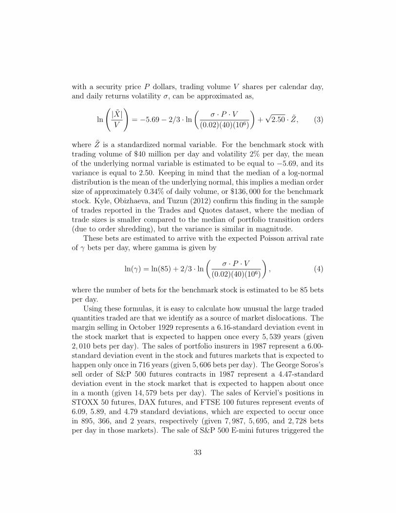
As discussed in Kyle and Obizhaeva (2011a), this intuition leads to simpleformulas for market depth and bid-ask spread as functions of observabledollar trading volume and volatility. The expected percentage price impactfrom buying or sellingX shares of a stock with a current stock price P dollars,expected trading volume V shares per calendar day, and daily percentagestandard deviation of returns σ (“volatility”), is given by
∆P (X)
P= exp
[λ/104 ·
(P · V40 · 106
)1/3
·( σ
0.02
)4/3· X
(0.01)V
]− 1. (1)
In this formula, the market impact parameter λ is scaled so that it measuresthe percentage market impact of trading X = 1% of expected daily volumeV of a hypothetical “benchmark stock” with stock price of $40 per share,expected daily volume of one million shares, and volatility of 2% per day. Theformula shows how to extrapolate market impact for the benchmark stockto assets with different levels of dollar volume and volatility. Microstructureinvariance also makes predictions about bid-ask spread costs. In the contextof significant market dislocations, bid-ask spread costs are so small relativeto impact costs that we ignore them in this paper.
We chose to consider continuously compounding returns rather than sim-ple returns as in Kyle and Obizhaeva (2011b), because our analysis dealswith very large orders, sometimes equal in magnitude to trading volume ofseveral trading days. In contrast, Kyle and Obizhaeva (2011a) consider rela-tively small portfolio transition orders with the average size of about 3.90%of daily volume and median size of 0.59% of daily volume; for these orders,the distinction between continuous compounding and simple compoundingis immaterial.
Kyle and Obizhaeva (2011b) estimate the the parameter λ = 5.78 basispoints (standard error 2 · 0.195), using data on implementation shortfall ofmore than 400,000 portfolio transition trades. A portfolio transition occurswhen one institutional asset manager is replaced by another. Trades con-verting the legacy portfolio into the new portfolio are typically handled by
7
a professional transition manager. Implementation shortfall, as discussed byPerold (1988), is the difference between actual execution prices and pricesbased on transactions-cost-free “paper trading” at prices observed in the mar-ket when the order is placed. Portfolio transition trades are ideal for usingimplementation shortfall to estimate transactions costs because the knownexogeneity of the size of the trades eliminates selection bias.
Formula (1) describes market impact during both normal times and timesof crash or panic, for individual stocks and market indices. Most of the eventsthat we consider in this paper occurred in markets with high trading volumeand during the times of significant volatility. For market with exceptionallyhigh trading volume and volatility, the market impact implied by equation(1) is greater than the impact obtained from the conventional heuristics.
The conventional wisdom about market impact can be illustrated by anaive implementation of the the formula λ = σV /σU from Kyle (1985). Underthe assumptions that the standard deviation of fundamentals σV is propor-tional to price volatility σ ·P and the standard deviation of order imbalancesσU is proportional to dollar volume V , the price impact can be calculated as
∆P (X)
P= exp
[λ/104 ·
( σ
0.02
)· X
(0.01)V
]− 1. (2)
According to the conventional wisdom in equation (2), increasing dollar vol-ume by a factor of 1, 000—approximately consistent with dollar volume dif-ferences between a benchmark stock and stock index futures—the impactof executing an order equal to a given percentage of expected daily volumedoes not change. According to microstructure invariance, the same increasein dollar volume increases the price impact of trading a given percentage ofaverage daily volume by a factor of (1000)1/3 = 10. The impact is ten timesgreater than conventional wisdom would predict. Also, according to con-ventional wisdom, doubling volatility doubles the market impact of tradinga given percentage of expected daily volume. According to microstructureinvariance, doubling volatility increases the price impact of trading a givenpercentage of expected daily volume by a factor of 24/3 ≈ 2.52.
When the effects of volume and volatility are taken into account, as sug-gested by the invariance hypothesis, we conclude that the observed marketdislocations could have been caused by selling pressure, because their effecton prices is much higher than conventional wisdom suggests. The executionof large bets—“small” relative to large overall trading volume—can lead to
8
significant changes of market prices, especially during volatile times. For ex-ample, if we extrapolate the prediction of a price impact of merely 5.78 basispoints for a trade of 1% of daily volume in the benchmark stock with dollarvolume of $40 million per day and volatility of 2% per day to a trade of 10%of daily volume in a stock index with dollar volume of $40 billion per day andthe same volatility of 2% per day (perhaps twice “normal” index volatilityof say 1% per day), we obtain a price impact of 578 basis points, consistentwith a major price dislocation. In this paper, we compare calculations of thisnature—calibrated to the volumes and volatilities observed in actual panicsand crashes—with the price dislocations observed.
In the last section of the paper, we also examine whether the frequencyof crashes and panics matches the predictions of invariance hypothesis.
Implementation Issues. In order to apply the model of market microstruc-ture invariance to the data on observed market dislocations, several imple-mentation issues need to be addressed.
First, it is necessary to identify the boundaries of the market, given thatdifferent securities and futures contracts, traded on various exchanges, mayshare the same fundamentals. For example, when a large order is placed inthe S&P 500 futures market, should the market volume include only S&P 500future volume, or should it also include volume in the 500 underlying stocks,stocks not part of the index, ETFs, index options, and other related mar-kets? Since a bet in S&P 500 futures contracts is a bet about the entire U.S.economy, it should be related to the markets for all other securities thoughsome factor structure. Thus, the volume and volatility inputs in our formulasshould not be thought of as parameters of narrowly defined markets of a par-ticular security in which the bet was placed, but rather as parameters frommuch broader markets. While at this time, we do not have a definitive under-standing of how to aggregate estimates across economically related marketsin the context of the invariance hypothesis, this is an interesting issue forfurther research.
Second, it is likely that the price impact of an order—especially its tran-sitory price impact— is related to the speed or aggressiveness with whichthis order is executed. Our market impact formula assumes that orders areexecuted at an appropriate speed in some “natural” units of time, with thespeed proportional to the speed with which the trading game itself is beingplayed. For example, a very large trade in a small stock may be executed over
9
several weeks, while a large trade in the stock index futures market might beexecuted over several hours. If execution is speeded up relative to a naturalflow of time, then our formula probably underestimates the expected cost.For unusually rapid execution of orders, we expect to see larger immediateprice impact than implied by our estimate from portfolio transitions data;moreover, we expect much of this impact to be transitory, reversing itselfsoon after the trade is completed.
Third, our price impact estimates are based on assumptions about the ex-pected volume and the expected volatilities prevailing during extreme events.We estimate volume and volatility based on historical data for recent monthsbefore the crash or panic event. During times of market stress, both volumeand volatility can increase. If higher levels of contemporaneous volume andvolatility are used to estimate price impact, the estimated impact will behigher as a result of the greater volatility and lower as a result of the greatervolume (holding the size of the order constant as a fraction of past volume).Whether unusually high volume or volatility at the time of order executionare associated with higher price impact is not well-understood. This is aninteresting issue for future research.
Fourth, while our market impact formula predicts expected price changes,the actual price changes reflect not only sales by particular groups of tradersplacing large bets but also many other events occurring at the same time,including arrival of news and trading by other traders. Our identifying as-sumption is that the effect of these forces on prices is zero. We also providea brief discussion of how other factors could have influenced market pricesduring the episodes we examine.
The remainder of this paper extrapolates the invariance model to examineseveral market dislocations.
2 The Stock Market Crash of October 1929
The October 1929 stock market crash is the most infamous crash in the his-tory of the United States. The crash of 1929 became seared in the memoriesof many because it is associated with the even more extraordinary decline instock prices which occurred from 1930 to 1932, subsequent bank runs, andthe Great Depression.
In the 1920s, many Americans became heavily invested in stocks. Inmany dimensions, stock market speculation in the late 1920s was similar to
10
stock speculation in the late 1990s. In the late 1920s, a significant portionof stock investments was made in margin accounts. After doubling in valueduring the two years prior to September 1929, the Dow Jones average fell by9% from 336.13 to 305.85 during the week before Black Thursday, October24, 1929, including a drop of 6.32% the day before. This steep price declineled to liquidations of stocks in margin accounts on the morning of BlackThursday. During the the first few hours of trading, the Dow Jones averagefell from the Wednesday closing value of 305.85 to 272.32, a decline of 11%.After a group of prominent bankers publicly announced steps to support themarket with significant purchases, the decline began to reverse itself. By theFriday close, October 25, 1929, the index recovered to 301.22, but confidencewas badly shaken.
Market conditions worsened the following week, with more heavy marginselling. On Black Monday, October 28, 1929, the Dow plummeted 13.47%,closing at 260.64. On Black Tuesday, October 29, 1929, the Dow fell anadditional 11.73%, closing at 230.07. Thus, over one week, the Dow fell byabout 25%. The slide continued for three more weeks, with prices reaching atemporary low point of 198.69 on November 13, 1929, about 48% below thehigh of 381.17 on September 3, 1929. During this period, the New York Fedbought government securities and cut its discount rate twice in an effort torestore confidence and provide liquidity to the financial system.
How much margin selling occurred during the week which included BlackThursday, Black Monday, and Black Tuesday? We follow the previous lit-erature by trying to estimate margin selling indirectly from data on brokerloans. Our research strategy is to use changes in broker loans during the fallof 1929 to infer the amount of margin selling of stocks. This research strategyin consistent with the way regulators and market participants looked at thesituation in the 1920s.1
In the 1920s, there was rapid growth in credit used to finance ownershipof equity securities. There was upward pressure on interest rates. Demandfor stocks shifted the supply of funds to the debt market down, while de-
1Our analysis is based on several documents: Federal Reserve Bulletins for 1929; AnnualReport of the Board of Governors of the Federal Reserve System 1926, 1927, 1928, 1929,and 1930; Monetary Statistics Book; “The Great Crash 1929” by John K. Galbraith(1954 and 1988); Pecora Commission Report (1934); “A Monetary History of the UnitedStates, 1867-1960” by Milton Friedman and Anna J. Schwartz (1963); “Margin Purchases,Brokers’ Loans and the Bull Market of the Twenties” by Gene Smiley and Richard H.Keehn (1988); and “Brokers’ Loans” by Lewis H. Haney (1932).
11
mand for leverage to finance stock investment increased demand for credit.To finance their purchases, individuals and non-financial corporations reliedeither on bank loans collateralized by securities or on margin account loansat brokerage firms.
When individuals and non-financial corporations borrowed through mar-gin accounts at brokerage firms, the brokerage firms financed a modest por-tion of the loans with credit balances from other customers. To finance thebalance, brokerage firms pooled securities pledged as collateral by customersunder the name of the brokerage firm (i.e., in “street name”) and then “re-hypothecated” these pools by using them as collateral for broker loans. Insome ways, the broker loan market of the 1920s played a role similar to theshadow banking system of the first decade of the 21st century. Similaritiesinclude the large size of the market, its lack of regulation, its perceived safety,and the large fraction of overnight or very short maturity loans.
High interest rates on broker loans—typically 300 basis points or morehigher than loans on otherwise similar money market instruments—were at-tractive to lenders. Banks supplied their funds to the market, with NewYork banks frequently acting as intermediaries arranging broker loans fornon-New-York banks and non-bank lenders. Instead of investing in commonstocks deemed to be overvalued, investment trusts, which played a role sim-ilar to closed end mutual funds today, also placed a large fraction of thenew equity they raised into the broker loan market. Finally, as a result ofgrowing earnings and proceeds of securities issuance, corporations possessedconsiderable cash balances. Attracted by high interest rates, some of themalso invested a large portion of these funds in the broker loan market ratherthan in new plant and equipment.
The broker loan market was controversial during the 1920s, just as theshadow banking system was controversial during the period surrounding thefinancial crisis of 2008-2009. Some thought the broker loan market shouldbe tightly controlled to limit speculative trading in the stock market on thegrounds that lending to finance stock market speculation diverted capitalaway from more productive uses in the real economy. Others thought it wasimpractical to control lending in the market, because the shadow bank lenderswould find ways around restrictions and lend money anyway. The New YorkFed chose to discourage banks from increasing broker loans and other loansfinanced collateralized by securities, and loans to brokers by New York banksdeclined after reaching a peak in 1927. This put upward pressure on brokerloan rates and attracted non-bank and foreign bank lenders into the market.
12
The non-bank lenders often bypassed the banking system entirely by makingloans to brokerage firms directly.
Market participants in the late 1920s watched statistics on broker loanscarefully, noting the tendency for broker loans to increase as the stock marketrose. Markets were also aware that margin account investors were buyerswith “weak hands,” likely to be flushed out of their positions by margincalls if prices fell significantly. They thought deeply about who the buyerswould be if a collapse in stock prices forced margin account investors out oftheir positions. Such discussions in 1929 mirrored similar discussions in 1987concerning who would take the opposite side of portfolio insurance trades.
Data on Broker Loans. In the 1920s, data on broker loans came from twosources. The Fed collected weekly broker loan data from reporting memberbanks in New York City supplying the funds or arranging loans for others,and the New York Stock Exchange collected monthly broker loan data basedon demand for loans by NYSE member firms. Our analysis of the broker loandata requires paying careful attention to both series, because the NYSE seriesis more complete in some respects, while weekly dynamics are also importantfor measuring selling pressure during the last week of October 1929.
Figure 1 shows the weekly levels of the Fed’s broker loan series and themonthly levels of the NYSE broker loan series. Two versions of each seriesare plotted, one with bank loans collateralized by securities added and onewithout. In addition, the figure shows the level of the Dow Jones IndustrialAverage from 1926 to 1930. The time series on both broker loans and stockprices follow similar patterns, rising steadily from 1926 to October 1929 andthen suddenly collapsing. According to Fed data, broker loans rose from$3.141 billion at the beginning of 1926 to $6.804 billion at the beginning ofOctober 1929. According to NYSE data, the broker loan market rose from$3.513 billion to $8.549 billion during the same period.
The Fed data do not include broker loans which non-banks made directlyto brokerage firms without using banks as intermediaries; such loans bypassedthe Fed’s reporting system. The broker loan data reported by the New YorkStock Exchange do include some of these broker loans. As more and morenon-banks were getting involved in the broker loan market, the differencebetween NYSE broker loans and Fed broker loans steadily increased untilthe last week of October 1929. This difference suddenly shrank afterwardsas these firms pulled their money out of the broker loan market. Since loans
13
unreported to the Fed were a significant source of broker loans and theseloans fluctuated significantly around the 1929 stock market crash, we relyrelatively heavily on the NYSE numbers in our analysis below.
During the period 1926 to 1930, the weekly changes in broker loans weretypically relatively small and often changed sign, as shown in the bars atthe bottom of figure 1. The last week of October 1929, which marked thebeginning of the stock market crash, and the first weeks of November 1929were significant exceptions. During these weeks, there were huge negativechanges almost twenty times larger than the average magnitude of changesduring other weeks. During a period of several weeks, this huge deleveragingreduced the level of broker loans back to the beginning of 1928.
Figure 2 shows what happened between September 4, 1929, and December31, 1929, in more detail. In the weeks leading up to the stock market crashduring the last week of October 1929, the reported Fed numbers were stable:$6.761 billion on September 25, $6.804 billion on October 2, $6.713 billion onOctober 9, $6.801 billion on October 16, and $6.634 billion on October 23.As the market crashed during the last week of October 1929, the quantityof broker loans reported by the Fed collapsed as well. Reported broker loansfell to $5.538 billion on October 30, $4.882 billion on November 6, $4.172billion on November 13, $3.587 billion on November 20, and $3.450 billionon November 27.
The monthly broker loans as reported by the NYSE were $8.549 billionon September 30, $6.109 billion on October 31, and $4.017 billion on Novem-ber 30. We estimate weekly values for the NYSE monthly time series bylinearly interpolating values from the weekly Fed series, with the exceptionof the critical month of October 1929. Based on the patterns of weekly Fednumbers during that month, we assume that the October decline in brokerloans occurred entirely during the last week of October. Thus, as measuredby the NYSE, broker loans fell by $2.340 billion during last week of Octoberand then by an additional $2.092 billion in November 1929, a total of about4% of 1929 GDP of $104 billion.
Immediately after the initial stock market break on Black Thursday, agroup of prominent New York bankers had put together an informal fundof about $750 million to provide support to the market. According to pressreports, the group did not intend to support prices at a particular floor, butrather intended to provide bids as prices fell, thus allowing the market to finda new level in an orderly manner. The group also appears to have supportedthe market by allowing the positions of large under-margined stock investors
14
to be liquidated gradually.While there was panic in the stock market during 1929 crash, there was
no observable financial panic in the money markets. In this respect, thepanic surrounding the 1929 stock market crash was entirely different fromthe panic surrounding the collapse of Lehman Brothers in 2008. From pastexperience pre-dating the establishment of the Fed in 1913, Wall Street wasfamiliar with financial panics in which fearful lenders suddenly withdrewmoney from the money markets, short term interest rates spike upwards,credit standards become more stringent, and weak borrowers were forced toliquidate collateral at distressed prices. In the last week of October 1929,interest rates actually fell and credit standards were relaxed by major banks,which cut margin requirements for stock positions. Some lenders abandonedthe broker loan market because falling interest rates made lending in thebroker loan market far less attractive than it used to be. The result wasan unprecedented spike in demand deposits at New York banks, which rosefrom $13.314 billion to $15.110 billion during the last week in October. Thisincrease in demand deposits conveniently gave the banks plenty of cash touse to finance increased loans on securities. The New York Fed encouragedeasy credit by purchasing government securities, by cutting the discount rate,and by encouraging banks to expand loans on securities to support an orderlymarket.
As reported in the Annual Reports of the Board of Governors of theFederal Reserve System 1929, bank loans on securities were relatively stablein the weeks leading up to the crash during the last week of October, rangingfrom $7.632 billion on September 4 to $7.920 billion on October 23. Duringthe week of the crash beginning on October 23, the level of bank loans onsecurities increased abruptly by $1.259 billion to $9.179 billion on October30. The sudden increase in bank lending was unprecedented. It also turnedout to be temporary. Loans on securities fell to $8.746 billion on November 6and $8.369 billion on November 13. In the latter half of November, loans onsecurities fell to around $7.900 billion, similar to the level at the beginningof October, and stayed at this level until the end of 1929.
The large increase in loans on securities is consistent with the interpre-tation that bankers took the financing of some under-margined accounts outof the hands of brokerage firms and brought the broker loans onto their ownbalance sheets. The gradual reduction in these loans over several weeks sug-gests that the bankers were liquidating these positions gradually in order toavoid excessive price impact and thus contributed to a more orderly market.
15
Instead of fire sale prices resulting from a credit squeeze, the picture was oneof a sudden, brutal bursting of a stock market bubble financed by prudentmargin lending to imprudent borrowers, with a rapid return to “normal”price levels in the stock market.
We define the time interval for the stock market crash of 1929 as the lastweek of October. The total reduction in brokerage loans during this weekwas approximately equal to $2.340 billion. The transfers of pledged collateralfrom brokerage firms to banks was equal to $1.259 billion. The amount ofmargin selling of stocks during that week can be therefore approximated by$1.181 billion ($2.340 billion minus $1.259 billion), slightly more than 1% of1929 GDP.
Our estimate of $1.181 billion of margin selling as the amount sold dur-ing the 1929 stock market crash assumes that every dollar in reduced marginlending represents a dollar of margin selling. In theory, it is possible formargin lending to fall for other reasons, including sales of bonds financed inmargin accounts and cash transfers from bank accounts to margin accountsat brokerage firms. We doubt that bond sales or transfers from bank accountswere significant during the last week of October 1929 because the high in-terest rate spread between broker loan rates and interest rates on bonds andbank accounts would have made it non-economical for investors to financebonds in margin accounts or to maintain extra cash balances at banks whilesimultaneously holding significant margin debt.
Market Impact of Margin Selling. For the purposes of examining theimplications of microstructure invariance, we define the 1929 crash period asthe last week of October, during which stock prices fell 24% and we estimatemargin sales of $1.181 billion. Are forced margin calls of $1.181 billion in thelast week of October 1929 massive enough to cause the observed downwardspiral in stock prices? To apply the price impact equation (1) to the 1929crash, we need to have estimates of dollar volume and volatility. We can thencompare the market price decline implied by microstructure invariance withthe historical price decline of 24% during the last week of October 1929. Ofcourse, this exercise provides only rough estimates for price changes, sincewe must make a number of simplifying assumptions.
To convert 1929 dollars to 2005 dollars, we use the GDP deflator of 9.42.We use the year 2005 as a benchmark, because the estimates in Kyle andObizhaeva (2011b) are based on the sample period 2001-2005, with more
16
observations occurring in the latter part of that sample. In the month prior tothe market crash, typical trading volume was reported to be $342.29 millionper day in 1929 dollars, or almost $3.22 billion in 2005 dollars. Prior to 1935,the volume reported on the ticker did not include “odd-lot” transactionsand “stopped-stock” transactions, which have been estimated to account forabout 30 percent of the “reported” volume. We therefore adjust reportedvolume by multiplying it by the fraction 10/7. Historical volatility the monthprior to October 1929 was about 2.00% per day. The total value of $1.181billion traded during the last week of October is approximately equal to 242%of average daily volume in the previous month.
The price impact equation (1) therefore implies that the forced margin-related sales of $1.181 billion triggered a price decline of 49.22%, calculatedas
1−exp[−5.78/104·
(488.98 · 106 · 9.42
(40)(106)
)1/3
·(0.0200
0.02
)4/3
· 1.181 · 109
(0.01)(488.98 · 106)
].
As a robustness check, table 2 reports other estimates using historical tradingvolume and volatility calculated over the preceding N months, with N =1, 2, 3, 4, 6, 12.
Table 2 shows the implied price impact of $1.181 billion of margin salesgiven a GDP deflator adjustment which equates $1 in 1929 to $9.42 in2005, along with average daily 1929 dollar volume and average dailyvolatility for N = 1, 2, 3, 4, 6, 12 months preceding October 24, 1929,based on a sample of all CRSP stocks with share codes of 10 and 11.
The actual market drop in the the last week of October 1929 was 24%,significantly less that our predicted price declines ranging from 31.05% to49.22%.
17
We estimate the total decline in broker loans during the last week ofOctober and the entire month of November to be the sum of the $2.340billion decline in broker loans during the last week of October 1929 and the$2.092 billion decline in broker loans in November 1929, implying a total of$4.432 billion in margin selling over five weeks. Netting out the temporaryincrease in bank loans financed by securities, our estimated margin selling of$1.181 billion during the last week of October is only about one fourth of thetotal estimate of margin selling for the entire five week period. Why did wenot see three more market crashes of similar magnitude in November 1929?We believe that there are three reasons that the market crash of 1929 mayhave been so well contained.
First, there was clearly significant cash waiting on the sidelines to be in-vested in stocks in the event stock prices fell significantly. Some of this cashrepresented stock issuance by investment trusts and non-financial corpora-tions.
Second, we believe that by spreading out the margin selling over a periodof five weeks instead of a few days, the financial system of 1929 reduced theprice impact which might otherwise have occurred.
Third, financial markets in 1929 may have been less integrated than today.For example, if we think of the stock market of 1929 as 125 separate marketsin different stocks, invariance implies that price impact estimates would bereduced by a factor of 1251/3 = 5.
Nevertheless, one of the main lessons learned from applying market mi-crostructure invariance to the 1929 crash is that financial markets in 1929appear to be very resilient when compared with today’s markets.
3 The Market Crash in October 1987
On October 14, 1987, the U.S. equity market began the most severe one-weekdecline in its history. The Dow Jones index dropped from about 2500 on themorning of Wednesday, October 14, 1987, to 1700 on Tuesday, October 20,1987, a decline of 32%. Even worse, S&P 500 futures fell from 312 on themorning of October 14, 1987, to 185 at noon on October 20, 1987, a declineof about 40%.
Some market observers blamed portfolio insurance for this dramatic de-crease in prices. Portfolio insurance was a trading strategy that replicated putoption protection for portfolios by dynamically adjusting stock market expo-
18
sure in response to market fluctuations. Since this strategy requires portfolioinsurers to sell stocks when stock prices fall, following the strategy indeedgenerates large sales in falling markets, thus amplifying downward pressureon prices. Most portfolio insurers traded stock index futures contracts toimplement the strategy. There has been a longstanding debate about theextent to which portfolio insurance trading contributed to the 1987 marketcrash.
An important question is therefore whether the size of sales by portfolioinsurers was large enough to create price impact that explains the magnitudeof price declines observed during the turbulent month of October 1987. Givenestimates of the selling pressure exerted on the markets by portfolio insurancesales, we use equation (1) to predict the price impact of portfolio insurancesales during the crucial days in October 1987. In order to calculate thepredictions, we need to make several assumptions related to measurement ofvolume and volatility.
First, the stock market crash of 1987 occurred during chaotic market con-ditions, the primary symptom of which was a dramatic increase in volatility.The spirit of the invariance hypothesis is that the volatility σ in the priceimpact equation (1) represents the volatility that investors expect. Thisvolatility determines the size of bets investors are willing to make and thedegree of market depth they are willing to provide. We assume that thechaotic conditions surrounding the stock market crash of 1987 are capturedby potentially high volatility estimates used as inputs into the formula. Notethat dramatically different price impact estimates are possible, dependingon whether volatility estimates are based on implied volatilities before thecrash, implied volatilities during the crash, historical volatilities based on thecrash period itself, or historical volatilities based on months of data beforethe crash.
Second, there have been numerous changes in market mechanisms be-tween 1987 and 2005, including changes in order handling rules in 1998 af-fecting NASDAQ stocks, a reduction in tick size from 12.5 cents to one cent,and the migration of trading in stocks and futures from face-to-face tradingfloors to electronic platforms. While such changes may have lowered the bid-ask spread component of transactions costs, we assume that they have hadlittle effect on market depth. This assumption makes it possible to applymarket depth estimates for 2001-2005 to the 1987 experience.
Third, the NYSE and NASDAQ markets for individual stocks are con-nected to index futures contracts by arbitrage relationships. Trading by
19
index arbitragers normally insures that the stock index futures market andthe cash market move closely together. Consistent with the spirit of theBrady report, we consider the futures market and the market for underlyingstocks to be one marketplace. We therefore measure trading volume in thecombined markets by simply adding together the dollar notional volume inthe futures market and the dollar value of stocks traded in the NYSE andNASDAQ. We calculate a market depth measure for the combined market.
Most portfolio insurance strategies were implemented by trading futurescontracts, providing “overlay” protection to an underlying portfolio of stocks.As heavy selling pressure in the futures markets pushed futures prices downrelative to stock prices in the cash markets, normal arbitrage relationshipsbroke down, and futures contracts became unusually cheap relative to thecash market. Many portfolio insurers abandoned their reliance on the futuresmarkets and switched to selling stocks directly.
Given that markets for underlying stocks also exchange idiosyncraticrisks, there is probably a more precise way to address the issue of how liquid-ity is aggregated across markets. A satisfactory theory should also addressthe issue of how liquidity is aggregated across correlated stock markets indifferent countries. During the stock market crash of 1987, stock indices fellin all major worldwide markets, indicating a systemic event of internationalproportions. The analysis the 1987 crash by Roll (1988) identified the world-wide nature of the crash as an issue indicating some force at work other thanthe selling pressure of portfolio insurance in the U.S. market alone. Boththe manner in which price pressure spreads among markets connected bystrong arbitrage relationships, such as index futures and underlying stocks,and the manner in which price pressure spreads across correlated marketsnot connected by strong arbitrage relationships, such as U.S. and Europeanstock markets, are important areas for theoretical and empirical research onmarket microstructure invariance. Currently, we do not have a detailed un-derstanding concerning how to aggregate market depth measures across cor-related markets. In this paper, we take the admittedly simplified approachof adding together cash and futures volume in the U.S., while ignoring stockmarkets in other countries.
Fourth, several news announcements on October 14, 1987, may have hada negative effect on prices. The filing of anti-takeover tax legislation inducedrisk arbitrageurs to sell stocks of takeover candidates. The announcement ofpoor numbers for the trade deficit for August 1987 also had a negative effect.These negative news announcements may themselves have sent prices lower,
20
providing a trigger for the portfolio insurance sales which followed.In the month prior to market crash, the typical daily volume in the S&P
500 futures market was equal to roughly $10.37 billion in 1987 dollars. TheNYSE average daily volume was $10.20 billion in 1987 dollars. After adjust-ing these numbers for realized inflation by multiplying by the GDP deflator of1.54 between 1987 and 2005, the trading volume in both markets was roughlyequal to $15.97 billion and $15.71 billion in 2005 dollars, respectively. In themonth prior to the crash, the historical volatility of S&P 500 futures returnswas about 1.35% per day. Similar estimates can be obtained from the‘Bradyreport (1988).
We reconstruct selling pressure induced by portfolio insurers from tablesin the Brady report (pp. 197-198). From Figure 13 and Figure 14, we obtainthe dollar volume of the largest traders on the NYSE: $257 million sold and$201 million bought on October 15, $566 million sold and $161 million boughton October 16, $1,748 million sold and $449 million bought on October 19,and $698 million sold and $863 million bought on October 20. From Figure 15and Figure 16, we obtain the dollar volume of the largest traders in S&P 500futures on the CME: $534 million sold and $71 million bought on October 14,$968 million sold and $109 million bought on October 15, $2,123 million soldand $109 million bought on October 16, $4,037 million sold and $113 millionbought on October 19, and $2,818 million sold and $505 million bought onOctober 20. Total sell order imbalances, defined as sell orders minus buyorders and aggregated over the time span from October 14, 1987, to October20, 1987, were $9.51 billion in the S&P 500 futures and $1.60 billion in theNYSE stocks in 1987 dollars. In 2005 dollars, these numbers correspond to$14.65 billion and $2.46 billion, respectively.
Some of the market participants classified as portfolio insurers in theBrady report abandoned their portfolio insurance strategies in mid-October1987. Instead of selling index futures and the NYSE stocks, as suggestedby their trading portfolio insurance strategies, they switched to buying thesesecurities with the hope of making profits by providing liquidity to othersin clearly distressed financial markets. We think that for the purpose ofanalyzing the effect of “true” portfolio insurers on the market prices, it ismore appropriate to leave aside purchases of portfolio insurers during thatperiod and consider only sales generated by this group, which amounted to$10.48 billion in the S&P 500 index futures and $3.27 billion in the NYSEstocks in 1987 dollars. The aggregate selling pressure of these sales—equal toabout 67% of one day’s volume in both markets during the previous month—
21
is predicted to lead to a price decline of 19.12%, obtained from equation (1)as
1−exp[−5.78/104·
((10.37 + 10.20) · 109 · 1.54
40 · 106
)1/3
·(0.0135
0.02
)4/3
· (10.48 + 3.27) · 109
(0.01)(10.37 + 10.20) · 109]
Table 3 reports, for robustness, other estimates based on historical trad-ing volume and volatility calculated over the preceding N months, withN = 1, 2, 3, 4, 6, 12. We also report separately price impact based on port-folio insurers’ gross sell orders and net sell order imbalances calculated assales minus purchases. The table shows that the estimated price impact ofportfolio insurers’ order imbalances ranges from -11.13% to -15.75%. Theestimated price impact of portfolio insurers’ sales ranges from -13.59% to-19.12%.
Sell Orders as % ADV 66.84% 63.28% 63.65% 67.82% 66.53% 70.33%Price Impact of Sell Orders 19.12% 16.20% 14.00% 13.59% 15.10% 15.60%Price Impact of Imbalances 15.75% 13.30% 11.47% 11.13% 12.39% 12.80%
Table 3 shows the implied price impact triggered by portfolio insurers’net order imbalances ($9.51 billion in S&P 500 futures market and$1.60 billion on the NYSE market) and their sell orders only ($10.48billion in S&P 500 futures market and $3.27 billion on the NYSEmarket) in 1987 dollar during the market crash in 1987, given aninflation adjustment converting $1 in 1987 to $1.54 in 2005, averagedaily dollar volume and average daily volatility based on N monthspreceding October 14, 1987, with N = 1, 2, 3, 4, 6, 12, for the S&P 500futures contracts and the sample of all CRSP stocks with share codesof 10 and 11.
Our predicted price impact is somewhat smaller than the astonishing price
22
drops of 32% in the cash equity market and 40% in the S&P 500 futures mar-ket observed during the 1987 market crash. The general similarity betweenpredicted and observed values, however, is consistent with our hypothesisthat heavy selling induced by program trading played a dominant role inthe tumultuous events of October 1987. The price impact may have beenamplified by negative information which triggered the crash and aggravatedby breakdowns in the market mechanism documented in the Brady report.
4 Trades of George Soros on October 22, 1987
People know George Soros as a prominent philanthropist and a successfulspeculator. One of his most famous trades was shorting the British Poundand “breaking the Bank of England” in September 1992, when he made al-most $2 billion. Not many people remember, however, that George Soros alsohad less cheerful days. One of them was Thursday, October 22, 1987, justthree days after the historic market crash of 1987. On that day, George Sorosdecided to sell a large number of S&P 500 futures contracts. The sale hasbeen attributed to pessimistic predictions by Robert Prechter, who forecastfurther declines in market prices based on similarities between market pat-terns during the 1929 crash and the 1987 crash. This transaction turned outto be so costly for George Soros that it made him think about withdrawingfrom active management of his Quantum Fund.
A CFTC report (January 1988, p.171) outlines the events of October 22,1987, without mentioning Soros by name. The December S&P 500 futurescontract closed at 258 on October 21, 1987. Approximately two minutesbefore the opening bell at 8:28 a.m. on October 22, a customer of the clearingmember submitted a 1,200-contract sell order at a limit price of 200, morethan 20% below the previous day’s close. The price plummeted all the wayto 200 over the first minutes of trading, at which point the sell order wasexecuted. At 8:34 a.m., a second identical limit order for 1,200 contractsfrom the same customer was delivered to the same broker and also executed.It was mentioned that these transactions liquidated a long position acquiredon the previous day at a loss of about 22 percent, or about $60 million in 1987dollars. Within minutes, S&P futures prices rebounded and, over the nexttwo hours, recovered to the levels of the previous day’s close. Those traderswho bought futures contracts providing liquidity minutes earlier could havequickly sold the contracts for enormous profits.
23
Within several days, the Quantum Fund, managed by George Soros,sued the broker Shearson Lehman Hutton for tipping off other traders inthe Chicago Mercantile Exchange’s S&P 500 futures pit about a big sell or-der. According to the claim, traders agreed to keep prices at artificiallylow levels while Quantum Fund’s large sell order was executed, as a resultwhich the allegedly illegal conspiracy made the fund lose $60 million. We usethe market microstructure invariance hypothesis to examine whether a 20%price impact is reasonable for execution of this order.
Two other events may have exacerbated the decline in prices in the morn-ing of October 22. First, when the broker executed the second order, hemistakenly sold 651 more contracts than the order called for. The oversoldcontracts were taken into the clearing firm’s error account and liquidated ata significant loss to the broker. Second, the CFTC report says that the sameclearing firm also entered and filled four large sell orders for a pension fundcustomer between 9:34 and 10:45 a.m., with a total of 2,478 contracts soldat prices ranging from 230 to 241. Remarkably, these additional orders arefor almost exactly the same size as Soros’s orders, a fact which suggest somesort of coordination or communication regarding the size of these unusuallylarge orders.
Since the S&P 500 contract size is equal to 500 multiplied by the valueof the S&P 500 index, one contract represented ownership of about $129,000with S&P level of 258. Soros sold 2400 contracts, which corresponds to about$309.60 million in 1987 dollars (about 2.29% of daily trading volume). Thehistorical volatility in the previous month was 8.63% per day and the averagedaily volume in S&P 500 futures market was $13.52 billion. These estimatesare very high because of the increase in realized volatility and volume duringthe preceding week, which included the crash day of October 19, 1987, as wellas other days with unusually high returns volatility. Note that in contrastto the analysis of the 1987 crash, our estimates are based only on what hashappened in the S&P 500 futures market, because we assume that the futuresmarket and cash market became disconnected during the short period whenthese orders were executed, as reflected by the basis falling to about -60points during that period. The price impact equation (1) predicts that thesale of 2,400 contracts—equal to 2.29% of average daily volume during theprevious month—would trigger price impact of 7.21%, obtained as
1− exp[− 5.78/104 ·
(13.52B · 1.54
40 · 106
)1/3
·(0.0863
0.02
)4/3
· 309.60 · 106
(0.01)(13.52 · 109)
].
24
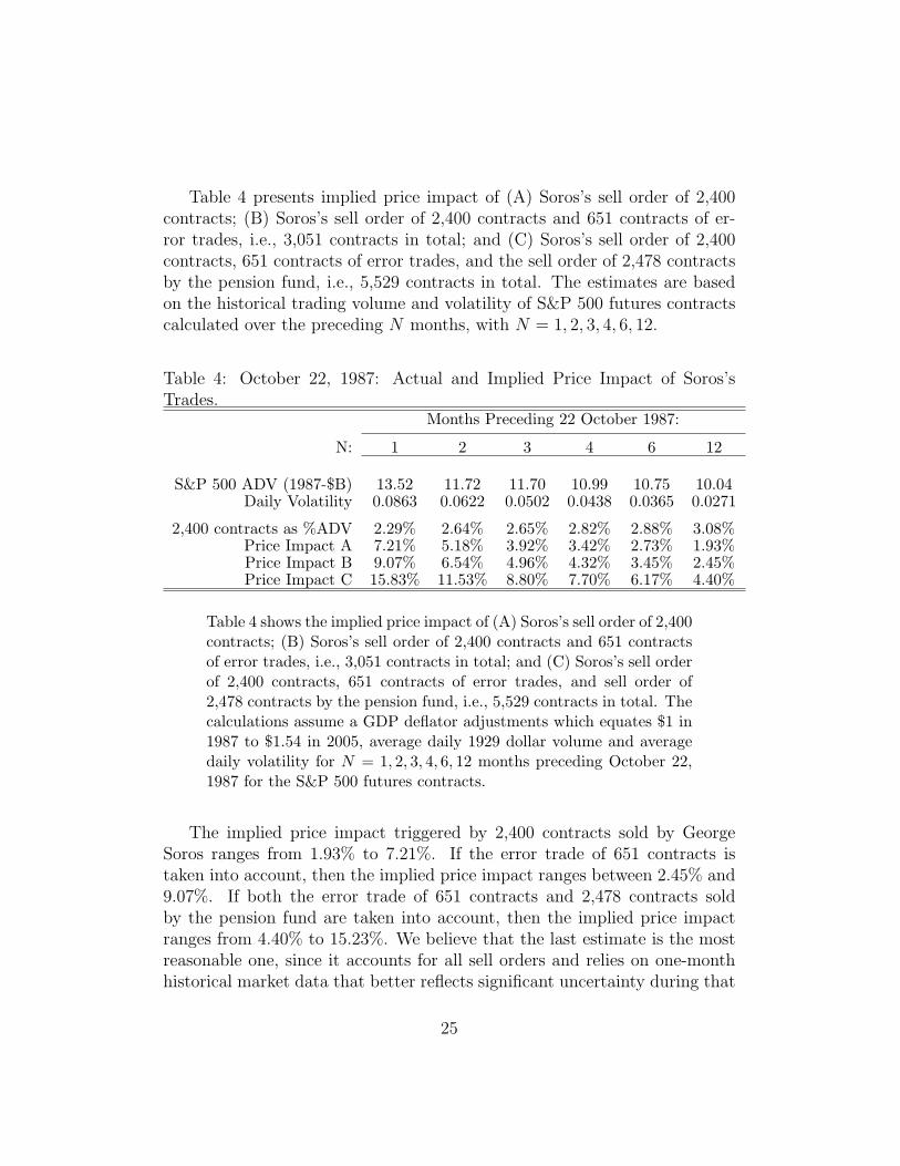
Table 4 presents implied price impact of (A) Soros’s sell order of 2,400contracts; (B) Soros’s sell order of 2,400 contracts and 651 contracts of er-ror trades, i.e., 3,051 contracts in total; and (C) Soros’s sell order of 2,400contracts, 651 contracts of error trades, and the sell order of 2,478 contractsby the pension fund, i.e., 5,529 contracts in total. The estimates are basedon the historical trading volume and volatility of S&P 500 futures contractscalculated over the preceding N months, with N = 1, 2, 3, 4, 6, 12.
Table 4: October 22, 1987: Actual and Implied Price Impact of Soros’sTrades.
2,400 contracts as %ADV 2.29% 2.64% 2.65% 2.82% 2.88% 3.08%Price Impact A 7.21% 5.18% 3.92% 3.42% 2.73% 1.93%Price Impact B 9.07% 6.54% 4.96% 4.32% 3.45% 2.45%Price Impact C 15.83% 11.53% 8.80% 7.70% 6.17% 4.40%
Table 4 shows the implied price impact of (A) Soros’s sell order of 2,400contracts; (B) Soros’s sell order of 2,400 contracts and 651 contractsof error trades, i.e., 3,051 contracts in total; and (C) Soros’s sell orderof 2,400 contracts, 651 contracts of error trades, and sell order of2,478 contracts by the pension fund, i.e., 5,529 contracts in total. Thecalculations assume a GDP deflator adjustments which equates $1 in1987 to $1.54 in 2005, average daily 1929 dollar volume and averagedaily volatility for N = 1, 2, 3, 4, 6, 12 months preceding October 22,1987 for the S&P 500 futures contracts.
The implied price impact triggered by 2,400 contracts sold by GeorgeSoros ranges from 1.93% to 7.21%. If the error trade of 651 contracts istaken into account, then the implied price impact ranges between 2.45% and9.07%. If both the error trade of 651 contracts and 2,478 contracts soldby the pension fund are taken into account, then the implied price impactranges from 4.40% to 15.23%. We believe that the last estimate is the mostreasonable one, since it accounts for all sell orders and relies on one-monthhistorical market data that better reflects significant uncertainty during that
25
day. This estimate is similar to but somewhat smaller than the price de-cline of 22% observed on the morning of October 22. Perhaps the expectedvolatility was higher than the one-month historical volatility. Perhaps theprice decline was exacerbated to the extent that some traders were indeed in-formed about existing requests to execute sale orders in the S&P 500 futuresmarket and profited from front-running based on this information. Also, thelarge price impact may be explained by the particular execution strategy ofGeorge Soros, who placed a limit sell order with a limit price of 200, substan-tially below the previous market close, signalling to the market the possibilitythat significant private information was behind the order.
5 The Liquidation of Jerome Kerviel’s Rogue
Trades by Societe Generale during January
21-23, 2008
On January 24, 2008, the Societe Generale issued a press release stating thatthe bank had “uncovered an exceptional fraud.” A trader, Jerome Kerviel,was accused of using “unauthorized” trading to take massive long positions,far beyond his limits in futures markets on major European indices.
According to the report of the investigation committee, Kerviel had es-tablished positions in index futures worth e50 billion: a e30 billion positionin futures on the STOXX 50, a e18 billion position in futures on DAX, anda e2 billion in futures on the FTSE 100. These positions were mostly ac-quired between January 2 and January 18, 2008. Kerviel had concealed hisfraud using fictitious trades, forged documents, and emails that misleadinglysuggested that all of his positions were hedged. The fall in index values inthe first half of January led to losses on his directional bets. The fraudu-lent positions were discovered on January 18. Their subsequent liquidationbetween January 21 and January 23 resulted in huge losses of e6.4 billionwhich, taking into account the e1.5 billion profit as of December 31, 2007,were reported as a global loss of e4.9 billion.
The Societe Generale shareholders, who were already concerned withlosses due to the bank’s exposure to subprime mortgages, were especiallydisappointed with additional losses incurred unwinding these fraudulent po-sitions. The bank officials blamed unfavorable market conditions, not themarket impact associated with liquidating the trades themselves, for the
26
large losses associated with liquidating the rogue positions.We examine whether the losses associated with price impact predicted by
our invariance model are consistent with actual reported losses and observeddeclines in prices. Answering this question again involves extrapolating ourinvariance model, estimated from portfolio transition trades in individualstocks, to the market for stock indices. Our estimates here are based on theassumption that the STOXX 50, the DAX, and the FTSE 100 are distinctmarkets. Treating them as one integrated market would also be reasonable,and would raise market impact estimates significantly, by more than 30%.
We first make assumptions about expected trading volume and returnsvolatility for futures on the STOXX 50, the DAX, and the FTSE 100 indices.In the month preceding January 18, 2008, historical volatility per day was98 basis points for futures on the STOXX 50, 100 basis points for futureson the DAX, and 109 basis points for futures on the FTSE. The estimatesof historical daily volume were e55.19 billion for STOXX 50 futures, e32.40billion for DAX futures, and £7.34 billion for FTSE 100 futures. Given theexchange rate of e1.3440 for £1 for January 17, 2008, Kerviel’s positions ofe30 billion in STOXX 50 futures, e18 billion in DAX futures, and e2 billionin FTSE 100 futures represented about 54%, 56%, and 20% of daily tradingvolume in these contracts, respectively.
According to the price impact equation (1), the liquidation of a e30billion position in STOXX 50 futures—equal to about 54.36% of the averagedaily volume in the previous month—is expected to trigger a price impact of14.34%,
1−exp[−2·2.89/104·
(55.19 · 1.4690 · 109
40 · 106
)1/3(0.0098
0.02
)4/330 · 109
(0.01)55.19 · 109],
In this equation, we use an exchange rate of $1.4690 per Euro to convert Eurovolume into U.S. dollar volume and a GDP deflator of 0.92 to convert 2008dollars into 2005 dollars. Similar calculations show that liquidation of e18billion in the DAX futures market had an estimated price impact of 12.75%and liquidation of e2 billion in FTSE futures had an estimated price impactof 4.81%. To obtain these numbers, we use the exchange rate of e1.3440 for£1 and $1.9744 for £1 on January 17. The predicted values are similar toobserved price changes. Indeed, the futures on the STOXX 50 fell by 10.50%from 4,028 to 3,605, the futures on the DAX fell by 11.91% from 7,379 to6,500, and the futures on FTSE fell by 4.65% from 5,895 to 5,621 during theperiod between January 18 and January 23, 2008.
27
Table 5 shows the estimates of price impact based on historical tradingvolume and volatility of futures on European indices calculated over thepreceding N months, with N = 1, 2, 3, 4, 6, 12.
Table 5: Societe Generale (2008): Implied Price Impact of LiquidatingJerome Kerviel’s Rogue Positions
Total Losses (2008-eB) 3.35 3.86 3.31 3.17 3.62 3.35Losses/Adj A (2008-eB) 5.66 6.17 5.62 5.48 5.93 5.66Losses/Adj B (2008-eB) 7.97 8.48 7.92 7.79 8.24 7.97
Table 5 shows the predicted losses of liquidating Kerviel’s positionsof e30 billion in STOXX 50 futures, e18 billion in DAX futures, ande2 billion in FTSE 100 futures, given an inflation adjustment of $1 in2008 equal to $0.92 in 2005, average daily volume of the futures on theSTOXX 50, the DAX, and the FTSE 100, and daily volatilities basedon N months preceding January 18, 2008, with N = 1, 2, 3, 4, 6, 12.
The official release reports losses of e6.30 billion. We assume that mar-ket predicted impact costs are equal to half of predicted price impact since,assuming no leakage of information about the trades, the trader can theo-retically walk the demand curve, trading only the last contracts at the worstexpected prices. Thus, invariance predicts transactions costs to be equal to
28
7.17% of the initial e30 billion position in STOXX 50 futures, 6.37% of theinitial e18 billion in DAX futures, and 2.40% of the initial e2 billion inFTSE futures. Altogether, the total cost of unwinding Kerviel’s position ispredicted to be e3.35 billion.
Since the official losses are calculated using the end of year 2007 prices asbenchmarks, we also adjust our estimates for losses on fraudulent positionsbetween December 31, 2007 and January 18, 2008, because the levels offutures prices dropped significantly during that period. From December 28,2007, to January 18, 2008, the futures on the STOXX 50 fell from 4,435 to4,028 (by 9.18%), the futures on the DAX fell from 8,144 to 7,379 (by 9.40%),and the futures on the FTSE fell from 6,455 on December 31, 2007, to 5,895on January 18, 2008 (by 8.68%).
If we assume that Kerviel acquired his positions gradually at averageprices from December 31, 2007, to January 18, 2008, then we have to addadditional losses of 9.18%/2 for STOXX 50 futures, 9.40%/2 for DAX futures,and 8.68%/2 for FTSE futures, i.e., e2.31 billion in total (“adjustment A”).The total loss of e3.35 billion adjusted for an additional e2.31 billion losswill then amount to about e5.66 billion, which is close to the reported lossesof e6.30 billion.
If, however, we assume that Kerviel acquired his position on December31, 2007, then the additional loss will be equal to 2· e2.31 billion, i.e., e4.62billion (“adjustment B”). The total loss of e3.35 billion adjusted for addi-tional the e4.62 billion loss reaches e7.97 billion, even higher than reportedlosses.
Table 5 reports estimates of total losses with both adjustments. The totalimplied trading costs range from e3.17 billion to e3.86 billion. The total losswith “adjustment A” ranges from e5.48 billion to e6.17 billion. The totalloss with “adjustment B” varies from e7.79 billion to e8.48 billion. Sincethese numbers are consistent with the losses of e6.30 billion reported bySociete Generale during liquidation of Kerviel’s positions, we conclude thatthese losses are consistent with the price impact of liquidating the tradesand should not be attributed to adverse market movements coincidentallyoccurring during the same period between January 21 and January 23, 2008.
There are two concerns that may affect our analysis. First, January 21,2008, was a holiday in the United States. In 2007, the futures markets hadonly one third of the typical volume on days when U.S. markets were closed.Lower trading volume on January 21 could have reduced market liquidity,making the unwinding of Kerviel’s positions more expensive. Second, the Fed
29
unexpectedly announced a substantial 75-basis point cut in interest rateson January 22, 2008, several days before its regularly scheduled meeting.This announcement had a positive effect on stock markets around the worldand should have helped Societe Generale to obtain more favorable executionprices on some portion of its trades.
6 The Flash Crash of May 6, 2010
Not all market crashes happen in the United States in October, and not allof them last for a long time. The flash crash of 2010 occurred on May 6 andlasted for only twenty minutes.
May 6, 2010, started with uncertainty concerning the debt crisis in Eu-rope, elections in the United Kingdom, and an upcoming jobs report in theUnited States. These worries led to growing uneasiness in the financial mar-kets. The S&P 500 declined by three percent during the first half of thatday. In the afternoon, something bizarre happened. The E-mini S&P 500futures contract suddenly fell from 1,113 at 2:40 p.m. to 1,056 at 2:45 p.m.,a decline of 5.12% over a five-minute period. Pre-programmed circuit break-ers built into the CME’s Globex electronic trading platform stopped futurestrading for five seconds. Over the next ten minutes, the market rose by about5%, recovering all of the earlier losses. This several-standard-deviation eventhappened so quickly that it could have been missed by those who steppedaway from their desks for a cup of coffee.
Shaken market participants began a search for guilty culprits. “Fat fin-ger” errors and a cyber attack were theories quickly discarded. Many accusedalgorithmic traders of failing to provide liquidity during the collapse of mar-ket prices.
After the flash crash, the CFTC and the SEC issued a joint report (May2010 and September 2010). The report suggested that the flash crash wastriggered by a single large sale of 75,000 contracts executed between 2:32 p.m.and 2:51 p.m. on the CME Globex platform via an automated executionalgorithm. The joint report of the CFTC and SEC did not mention thename of the seller, but journalists identified the large seller as Waddell &Reed. Given the value of S&P 500 at that time and a multiplier of $50, thesize of order was approximately $4.37 billion.
Many people did not believe the report’s suggestion that selling 75,000contracts could have triggered a price drop of 5%. Indeed, the order repre-
30
sented only 3.75% of the daily trading volume of about 2,000,000 contractsper day. A legitimate question is whether the execution of an order of thissize could have resulted in a flash crash associated with a 5% drop in prices.
To apply the market impact equation (1), we first need to make assump-tions about expected trading volume and volatility. Given a multiplier of 50,one S&P 500 E-mini contract represents ownership of about $58,200, with anS&P level of 1,164 on May 5, 2010. During the preceding month, the averagetrading volume was about $132 billion per day in 2010 dollars. Not surpris-ingly, the trading volume was much higher on May 6, 2010. The historicalvolatility was about 1.07% per day. Since volatility on May 6 was higherthan usual due to the European debt crisis, we also use a rough estimate ofexpected volatility equal to 2.00% per day. Given a GDP deflator of 0.90between 2005 and 2010, equation (1) implies that the order—equal to about3.31% of average daily volume in the previous month—implies a price declineof 2.71%, obtained as
Table 6 shows additional estimates based on historical trading volume andvolatility of S&P 500 E-mini futures contracts calculated over the precedingN months, with N = 1, 2, 3, 4, 6, 12, as well as a higher expected volatilityassumption of 2% per day.
The predicted price impact is smaller than the actual decline in prices of5.12%, but its magnitude is still substantial, especially if expected volatilitywas much higher than the historical one during that day. The estimates basedon historical volatility range from 0.88% to 1.49%. The estimates based ontwo-percent volatility range from 2.71% to 3.35%. Although 75,000-contractorder may seem to be only a small fraction of two million contracts of E-ministraded each day, its magnitude is much larger than that of other orders, andits execution therefore would demand substantial amount of liquidity.
Our estimates of price impact for the flash crash focus only on the futuresmarket. A better methodology would treat the cash market and the futuresmarket as one market. The result would be higher levels of expected tradingvolume and even lower price impact estimates, probably by about 35%.
Note that our estimates may underestimate actual price changes, since theprice impact parameter estimated from portfolio transition trades assumesthat trades are executed at a natural speed consistent with the manner in
31
Table 6: Flash Crash of May 6, 2010: Implied Price Impact of Large 75,000Contract Futures Sale.
Table 6 shows the predicted price impact of 75,000 S&P 500 E-minifutures contracts, given an inflation adjustment equating $1 in 2010to $0.90 in 2005, average daily volume and volatility of the S&P 500E-mini futures based on N months preceding January 18, 2008, withN = 1, 2, 3, 4, 6, 12.
which portfolio transition trades are executed. We believe that marketdepth is influenced by the speed of trading. The joint report indicates thatthe speed of execution of this large order over such a short period of time wasunusually fast for the the S&P 500 E-mini futures contract. We believe thatthe unusually rapid execution of this order probably led to much higher priceimpact than predicted from the market impact equation (1). A severe pricedecline immediately followed by a rapid price recovery is consistent with thishypothesis.
7 The Frequency of Market Crashes
Two questions immediately come to mind of worried investors and regulators.How unusual are large bets in financial markets? How often do they lead tocrashes and mini-crashes?
Large orders may be placed into the marketplace more often than tradersusually think. Using portfolio transitions data, Kyle and Obizhaeva (2011a,2011b) find that distributions of buy and sell order sizes can be closely ap-proximated by a log-normal with the mean that depends on the dollar volumeand volatility of the stock. The distribution of order sizes X of a security
32
with a security price P dollars, trading volume V shares per calendar day,and daily returns volatility σ, can be approximated as,
ln
(|X|V
)= −5.69− 2/3 · ln
(σ · P · V
(0.02)(40)(106)
)+√2.50 · Z, (3)
where Z is a standardized normal variable. For the benchmark stock withtrading volume of $40 million per day and volatility 2% per day, the meanof the underlying normal variable is estimated to be equal to −5.69, and itsvariance is equal to 2.50. Keeping in mind that the median of a log-normaldistribution is the mean of the underlying normal, this implies a median ordersize of approximately 0.34% of daily volume, or $136, 000 for the benchmarkstock. Kyle, Obizhaeva, and Tuzun (2012) confirm this finding in the sampleof trades reported in the Trades and Quotes dataset, where the median oftrade sizes is smaller compared to the median of portfolio transition orders(due to order shredding), but the variance is similar in magnitude.
These bets are estimated to arrive with the expected Poisson arrival rateof γ bets per day, where gamma is given by
ln(γ) = ln(85) + 2/3 · ln(
σ · P · V(0.02)(40)(106)
), (4)
where the number of bets for the benchmark stock is estimated to be 85 betsper day.
Using these formulas, it is easy to calculate how unusual the large tradedquantities traded are that we identify as a source of market dislocations. Themargin selling in October 1929 represents a 6.16-standard deviation event inthe stock market that is expected to happen once every 5, 539 years (given2, 010 bets per day). The sales of portfolio insurers in 1987 represent a 6.00-standard deviation event in the stock and futures markets that is expected tohappen only once in 716 years (given 5, 606 bets per day). The George Soros’ssell order of S&P 500 futures contracts in 1987 represent a 4.47-standarddeviation event in the stock market that is expected to happen about oncein a month (given 14, 579 bets per day). The sales of Kerviel’s positions inSTOXX 50 futures, DAX futures, and FTSE 100 futures represent events of6.09, 5.89, and 4.79 standard deviations, which are expected to occur oncein 895, 366, and 2 years, respectively (given 7, 987, 5, 695, and 2, 728 betsper day in those markets). The sale of S&P 500 E-mini futures triggered the
33
flash crash in 2010 represent 4.56-standard deviation event that is expectedto occur several times during a year given almost 11, 592 bets per day in thatmarket.
These calibrations suggest that large bets associated with crashes appearmore frequently than the log-normal distribution with the estimated varianceof 2.50 would imply. There may be several explanations of why the right tailof bet size distribution is fatter than predicted.
First, the calibrated standard deviation of bets from portfolio transitionsdata may be too small due to unique features of portfolio transitions. Otherinstitutional trades may be better approximated by a log-normal distributionwith bigger variance. Note, however, that a normal distribution impliesthat a 5-standard deviation event is 291 times more likely than a 6-standarddeviation event. Increasing the estimated standard deviation of 2.501/2 =1.58 by 20%, so that 6-standard deviation events would become 5-standarddeviation events, would imply that market crashes occur far too frequently.The true standard deviation may be higher by about 15%.
Second, the far right tail of the distribution of bets may be better de-scribed by a power law than a log-normal. Indeed, Kyle and Obizhaeva(2011b) find a slight deviation from the log-normal distribution for the verylargest portfolio transitions orders in most active stocks.
Thinking more about these alternatives is an important agenda for futureresearch in market microstructure.
8 Conventional Wisdom and Animal Spirits
Since before the 1929 crash, economists and market participants have beenpuzzled by why market crashes occur in the apparent absence of fundamentalinformation. There have long been two camps of thinking, which we willrefer to as “conventional wisdom” and “animal spirits.” Neither of these twotheories offers an explanation for crash events.
Conventional Wisdom. Conventional wisdom holds that prices react tochanges in fundamental information, not to the price pressure resulting fromtrades by individual investors. In the 1960s and 1970s, this conventionalwisdom became associated with efficient markets hypothesis and the capitalasset pricing model.
34
The efficient-market hypothesis is consistent with the idea that investorstrade for various reasons including portfolio rebalancing motives and profitingfrom private information. Since many investors are competing for informa-tion, however, one interpretation of the efficient markets hypothesis is that itwould be highly unusual for investors to have private information of sufficientvalue that the information content of their trades would move prices signif-icantly. Competitive markets with minimal private information thus implyminuscule price impact. Consistent with this theory, Scholes (1972) reportsthat relatively large blocks may be sold at approximately prevailing marketprices.
Conventional wisdom based on the CAPM implies that the demand formarket indices is very elastic. It also implies that the demand for individualstocks is almost infinitely elastic. The quantities observed changing hands inthe market are too small compared to trading volume or shares outstandingand their effect on prices can not explain dramatic plunges in market prices.
Views consistent with the conventional are shared by many prominenteconomists, including Merton H. Miller. Miller (1991), for example, wrotethe following about the 1987 crash: “Putting a major share of the blame onportfolio insurance for creating and overinflating a liquidity bubble in 1987is fashionable, but not easy to square with all relevant facts... No studyof price-quantity responses of stock prices to date supports the notion thatso large a price increase (about 30 percent) would be required to absorb somodest (1 to 2 percent) a net addition to the demand for shares.”
As the academics most associated with portfolio insurance, Leland andRubenstein (1988) echo this argument: “To place systematic portfolio in-surance in perspective, on October 19, portfolio insurance sales representedonly 0.2 percent of total U.S. stock market capitalization. Could sales of1 in every 500 shares lead to a decline of 20 percent in the market? Thiswould imply a demand elasticity of 0.01—virtually zero—for a market oftenclaimed to be one of the most liquid in the world.”
The Brady report (1988) compares the market crashes of 1929 and 1987and comes to similar conclusions about the 1929 crash: “To account for thecontemporaneous 28 percent decline in price, this implies a price [elasticity]of 0.9 with respect to trading volume which seems unreasonably high. Asa percentage of total shares outstanding, margin-related selling would havebeen much smaller. Viewed as a shift in the overall demand for stocks,margin-related selling could have accounted realistically for no more than 8percent of the value of outstanding stock. On this basis, the implied elasticity
35
of demand is 0.3 which is beyond the bound of reasonable estimates.”Brennan and Schwarz (1987) note that portfolio insurance would have a
minimal effect on prices, because most portfolio-consumption models implyelasticities of demand for stock more than 100 times the elasticities observedduring the 1987 crash. Many observers of the 1987 stock market crash,including Miller (1988) and Roll (1988), looked therefore to explanationsother than the price pressure of the large quantities traded to explain thelarge changes in prices. For all five crash events, however, it is difficult tofind new fundamental information shocks to which market prices would havereacted with the magnitude of price declines actually observed.
We disagree with the conventional wisdom on the grounds that the con-ventional wisdom of low price impact is empirically incorrect. Large trades,even those known to have no information content such as the margin sales of1929 or the portfolio insurance sales in 1987, do have large effect of prices.Our examination of five historical episodes suggests that actual price changesare similar to those predicted by the invariance formula. Indeed, the invari-ance price-impact model performs well when extrapolating from portfoliotransition trades in normal markets for individual stocks to unusually largebets in market indexes.
Animal Spirits. Animal spirits holds that price fluctuations occur as aresult of random changes in psychology, which may not be based on infor-mation or rationality. The term “animal spirits” was coined in by Keynes(1936) who says that most of our decisions can be taken only as the resultof “animal spirits—a spontaneous urge to action rather than inaction, andnot as the outcome of a weighted average of quantitative benefits multipliedby quantitative probabilities.” Shiller and Akerlof (2009) recently advocatedfor this theory again: “To understand how economies work and how we canmanage them and prosper, we must pay attention to the thought patternsthat animate peopole’s ideas and feelings, their animal spirits.” Accordingto animal spirit theory, market crashes are times when decisions are drivenby emotions and social-psychologically induced changes in mind set insteadof rational calculations. Promtly after the 1987 crash, for example, Shiller(1987) surveyed traders and found that “most investors interpreted the crashas due to the psychology of other investors.”
We disagree with animal spirits theory. Animal spirits suggests randomunpredictable nature of stock market crashes. In reality, large crashes are nei-
36
ther random nor unpredictable. The possibility of crashes is often discussedbefore crashes occur. For example, brokers were raising margins before the1929 stock market crash in order to protect themselves from increases in ex-pected market volatility. The SEC, worried that portfolio insurance madethe market fragile, did the study of portfolio insurance before the 1987 crashhappened. Smaller events like the sales of George Soros in 1987, the liqui-dation of fraudulent position by Societe Generale, and the flash crash wereunpredictable, but prices rapidly mean-reverted. Ironically, the more pre-dictable the crash is, the more permanent the price impact it triggers.
Stock Market Crashes and Banking Crises. The five stock marketcrashes discussed in this paper differ from the long-lasting financial crisescatalogued by Reinhart and Rogoff in This Time Is Different (2009). Thecrises examined by Reinhart and Rogoff include sovereign defaults, bankingcrises associated with collapse of the banking system, exchange rate crisesassociated with currency collapse, and bouts of high inflation. Reinhart andRogoff document that it usually takes many years and significant changesin macroeconomic policies and market regulations for the affected economiesto recover from these fundamental problems associated with insolvency offinancial institutions underlying the economy.
In contrast, stock market crashes or panics triggered by large bets arelikely to be short-lived if followed by appropriate government policy. Forexample, the Federal Reserve System implemented an appropriately loosemonetary policy immediately after the 1929 crash, which calmed down themarket by the end of 1929. The great depression of the 1930s resulted fromsubsequent deflationary policies associated with the gold standard, not the1929 crash. In the liquidation of Jerome Kerviel’s rogue trades in 2008, theimmediate 75-basis point interest rate cut by the Fed probably prevented thisevent from immediately spiraling into a deeper financial crisis, but it did notprevent the collapse of Bear Stearns a few weeks later. It was the bursting ofthe real estate credit bubble, not the unwinding of Jerome Kerviel’s fraud,that led to the deep and long-lasting recession which unfolded in 2008-2009.
We believe that the impact of events like the crashes and panics discussedin this paper can be reduced, if regulators systemically monitor market con-ditions to create awareness of the possibility that large bets are imminentand if market participants learn to appreciate that large bets will inevitablylead to large price impact. A good example is the 1987 stock market crash.
37
The SEC was aware that large trades by portfolio insurers were possible, butboth regulators and market participants were surprised by the large price im-pact resulting from entirely predictable attempts to execute the strategy infalling markets. Our simple and easily implemented methodology is designedto predict systemic stock market crash events in advance, using volatility andvolume from historical daily data.
9 Lessons Learned
It is, of course, impossible to infer from only five data points definitive con-clusions about the ability of microstructure invariance to predict the priceimpact of liquidations of large quantities of stock. Each of the crash eventsmay involve event-specific features which make it difficult to estimate the sizeof the positions liquidated, long-term volume and volatility, and the effectsof other contemporaneous events that may have affected market conditions.Application of microstructure invariance concepts to intrinsically infrequenthistorical episodes therefore requires an exercise in judgement to extract ap-propriate lessons learned. Nevertheless, the five cases we have examined sug-gest important lessons, both for policymakers interested in measuring andpredicting crash events of a systemic nature and for asset managers inter-ested in minimizing market impact costs associated with execution of largetrades that might potentially disrupt markets.
Large Price Impact in Liquid Markets. For the five crash events exam-ined in this paper, the predicted declines are large and similar in magnitude towhat actually occurred. The predicted declines for the 1929 crash, the 1987crash, the 1987 Soros trades, the 2008 Societe Generale trades, and 2010flash crash were 49.22%, 19.12%, 7.21%-15.83%, 4.75%-13.82%, and 1.19%-2.71%, respectively. Based on intra-period minimum prices reached, the ac-tual crash percentages were 24%, 32%-40%, 22%, 4.65%-11.91%, and 5.12%,respectively. This is consistent with the interpretation that microstructureinvariance may apply not only to individual stocks but also to stock index fu-tures markets or a combination of futures and cash markets. Microstructureinvariance implies that liquidating a given fraction of average daily volumehas larger price impact in markets with high volume and high volatility thanin markets with low volume and low volatility.
Furthermore, in contrast to models and empirical literature suggesting
38
that price impact is concave in trade size, microstructure invariance is basedon the maintained assumption that price impact is linear, even for very largetrades. Both of these features of microstructure invariance tend to mag-nify the estimated price impact of liquidations of large quantities of stockwhen crash events occur. The large predicted magnitudes suggest that bothincreasing price impact as volume increases (using a cube root) and linearprice impact are reasonable assumptions to apply to the stock market as awhole, not just individual stocks.
Speed of Liquidation Magnifies Short-term Price Effects. In thecrash events we have examined, the large sellers executed trades at differentspeeds. The 1987 Soros trades and the 2010 flash crash crash trades wereexecuted very fast, in minutes. The 1987 portfolio insurance trades and the2008 Societe Generale trades were executed more slowly, in a few days. The1929 crash trades were spread out over a long period of time, several weeks.
It is probable that the speed of execution influences the way in whichorders affect prices. If trades are executed very rapidly, there is likely tobe greater temporary price impact but not greater permanent impact. Thisimplies that trades executed rapidly are likely to generate a V-shaped pricepath, with price plunging rapidly, then recovering quickly. For the V-shapedprice path not to make it easy for others to profit from “front-running” thetrades, it is also necessary for the execution of such trades to be accompaniedby a dramatic, transitory increase in price volatility. Both the 1987 Sorosepisode and the 2010 flash crash are consistent with this hypothesis that veryrapid execution of trades generates high volatility and rapid mean reversionin prices.
The rapid execution of these trades may also partially explain why theactual price impact in some cases was greater than predicted by microstruc-ture invariance. Price impact parameters for microstructure invariance wereestimated based on portfolio transition trades, which are typically executedover a period of several days to a week or more in liquid and illiquid stocks.Since portfolio transition managers have extensive experience based on per-forming thousands of transitions, it is reasonable to assume that the timehorizons over which these trades are executed is sufficiently long to avoidextra market impact costs associated with executing trades very impatiently.In other words, portfolio transition trades are likely executed at a reasonable,prudent pace designed to keep price impact costs low. Obizhaeva (2008) doc-
39
uments some mean reversion months after portfolio transition sell trades, butthe mean reversion is rather small, consistent with permanent price impactassociated with positive information content of buy orders.
To reduce transitory impact costs associated with arbitragers “front-running” large orders, traders have an incentive to slow down executionenough so that the presence of the order is difficult to detect. What is areasonable speed at which to execute large trades? We can illustrate howmicrostructure invariance approaches this issue using the flash crash as anexample. Microstructure invariance is based on the intuition that “businesstime” passes more quickly for markets with higher levels of trading activity,defined as the product of dollar volume and volatility. To quantify this in anintuitive manner, we make intuitive back-of-the envelope calculations basedon round numbers (using powers of 2).
In the month prior to the flash crash, a reasonable round number estimateof daily dollar volume for the S&P E-mini contract is $128 billion per day(similar to average daily volume of $132 billion in table 6). A typical liquidstock on the NYSE has a volume of about $2 billion per day, approximately64 times less than stock index futures. Although historical S&P 500 volatilitywas less than 2% per day prior to the flash crash, our estimated price impactof 2.71% was based on a volatility estimate of 2% per day because of theunusually volatile conditions which occurred during morning trading, priorto the early afternoon flash crash on May 6, 2010. The volatility of anindividual liquid stock is not very different from 2% per day. This impliesthat the S&P 500 E-mini contract, under volatile conditions with 2% dailyvolatility, has trading activity approximately 64 times greater than a typicallarge liquid stock.
Applying exponents of 2/3 and 1/3 to 64, microstructure invariance im-plies that business time in the S&P 500 E-mini market should pass 16 timesfaster than for the individual liquid stock, and orders for the futures contractshould be 4 times larger than for the individual liquid stock. This impliesthat the probability of a flash crash order for about $4 billion dollars oc-curring on a given day is 16 times greater than an order for $1 billion in aliquid stock. This also implies that the flash crash order should be executed16 times more rapidly than an order for $1 billion in a liquid stock. Forexample, in the market for a liquid stock, it may be reasonable to execute anorder for $1 billion, or 50% of average daily volume, over 16 days, i.e., about3% of average daily volume for 16 consecutive days. This intuition impliesthat a $4 billion order in S&P futures, or 3% of average daily volume, would
40
be expected to be executed over a period of one day. The actual execution ofthe flash crash order occurred over a period of about 20 minutes, far fasterthan spreading the execution out over one day. This fast execution may haveamplified the transitory impact of executing this order, leading to temporaryprice impact of 5.12%, greater than our estimate of 2.71%. Kirilenko et al.(2012) draw a similar conclusion based on typical execution of large ordersin the stock index futures market. Note that Soros placed a sell limit orderbelow a bid in 1987 and executed his trade very quickly at the very beginningof the trading day. In both cases, there was a very high transitory volatility, avery rapid drop in prices, but very rapid almost immediate recovery minuteslater.
The 1987 portfolio insurance trades and the 2008 Societe Generale tradeswere executed quickly, over a few days, but not over weeks. The actual pricechanges during these episodes are similar to price changes predicted by theinvariance hypothesis based on the estimates from portfolio transitions. The1929 margin-related trades triggered price impact smaller than predicted byinvariance. As we explained above, measures implemented by bankers andregulators in the last week of October 1929 smoothed the margin selling outover a period of five weeks rather than a few days.
The main lesson is that slower execution of large trades would lessentemporary price impact and reduce transitory volatility. One obvious rea-son is that slow execution separates trades based on short-half-life privateinformation from liquidity trades. For example, trades in the 1929 crash,the 1987 crash and during liquidation of Societe Generale’s trades in 2008were certainly liquidity trades. While the 2010 flash crash trades may bethought to have private information, this information probably was not bebased on a 15-minute rumor. Soros explained his trades in 1987 by referringto Prechter’s Elliot Wave Theory, something which takes place over a longperiod of time.
The Financial System in 1929 Was Remarkably Resilient. The 1987portfolio insurance trades of $13 billion were equal to about 0.28% of GDP inthat year (1987 GDP was $4.7 trillion). Execution of these trades triggereda price impact of 32% in the “cash” stock market and 40% in the futuresmarket. The 1929 margin-related sales of $1.181 billion during the last weekof October were equal to 1% of GDP in that year (1929 GDP was $104billion). These margin-related sales were followed by additional sales equal
41
to 3% of GDP in subsequent weeks. Even though the sales of 1% of GDPwere almost four times larger than the 1987 portfolio insurance trades, theirexecution changed prices by only 24%. The financial system in 1929 wasremarkably resilient.
As market prices were falling in October 1929, several bankers got to-gether to formulate a common plan to stabilize market prices. The bankersquickly assembled a fund of $750 million to buy securities in order to supportprices. Their decisions were publicized, and the panic stopped. These meet-ings were not unprecedented. Similar actions, for example, were undertakenby J.P. Morgan and other bankers who stabilized the market in 1907 crash. Ifsuch meetings were to happen today, they would likely raise anti-trust issues.
The New York Fed also acted prudently. In the 1920s, bankers and theirregulators were aware that if non-bank lenders suddenly withdrew funds fromthe broker loan market, there would be pressure on the banking system tomake up the difference. By discouraging banks from lending into the brokerloan market prior to the 1929 crash, the New York Fed increased the abilityof banks to support the broker loan market after the stock market crashed.During the last week of October 1929, the New York Fed wisely reversedits course and encouraged banks to provide bank loans on securities to theirclients as a substitute for broker loans. At the same time, many brokers cutmargins from 40% to 20% on their loans to avoid immediate execution.
These actions created a space for the financial system to adjust over aperiod of about five weeks rather than a few days. One possible effect was toreduce the short-term impact of liquidations of margin loans by spreading theexecution of the trades out over time. Consistent with this hypothesis, we findthat during the 1929 crash, the actual price impact of 24% was small relativeto predicted price changes of 49.22%. The stock market prices stabilize bythe end of 1929. There were no major failures of banks or brokerage firms.
Early Warning Systems May Be Useful and Practical. Two events—1929 margin sales and 1987 portfolio insurance—involved aggregating tradesby numerous entities. In both cases, data was publicly available before thecrash event. Data on broker loans was published by the Federal ReserveSystem and the NYSE. Estimates of assets under management by portfolioinsurers were available before the 1987 crash, and sizes of potential sales werediscussed. In both cases, potential price impacts of liquidations were topicsof conversation among policy makers and market participants.
42
For example, the debate about the extent to which portfolio insurancetrading contributed to the 1987 market crash started before the crash itselfoccurred. The term “market meltdown,” popularized by then NYSE chair-man John Phelan, was used in the year or so before the stock market crashto describe a scenario of cascading sell orders resulting in severe price de-clines posing systemic risks to the economy. In the summer of 1987, theSEC conducted a study of a cascading meltdown scenario before the crashitself, reported in “Program trading: Hearing before the Subcommittee onTelecommunications and Finance of the Committee on Energy and Com-merce.” After describing in precise detail what a market crash would looklike, the study dismissed the risk of a crash as a remote possibility, in agree-ment with conventional Wall Street wisdom at the time.
Conventional wisdom has held that, given the substantial trading volumein the U.S. equity markets, and especially the index futures market, there wasenough liquidity available to accommodate sales of portfolio insurers withoutany major downward adjustment in stock prices. During the same hearingsin the summer of 1987, for example, Hayne E. Leland defended portoflioinsurance: “We indicated that average trading will amount to less than 2%of total stocks and derivatives trading. On some days, however, portfolioinsurance trades may be a greater fraction... In the event of a major one-dayfall (e.g., 100 points), required portfolio insurance trades could amount to $4billion. Almost surely this would be spread over 2-3 day period. In such acircumstance, portfolio insurance trades might approximate 9-12% of futurestrading, and 3-4% of stock plus derivatives trading.”
In both 1929 and 1987, regulators could theoretically have used our simplemethodology to better assess the potential size of a stock market crash.
Nowadays, a similar analysis may be required to analyze the effect of lever-aged ETFs on financial markets, an interesting topic for further research.
10 Conclusion
Financial markets are vulnerable to large plunges resulting from the execu-tion on unusually large bets. This point is consistent with the observationsof Fischer Black (1971), who believed that the execution of large orders willalways exert an impact on prices, regardless of technological advances inmarket microstructure and methods of execution.
Our use of market microstructure invariance to examine five stock market
43
crashes in this paper suggests that market depth is less than many tradersthink, especially for the largest and deepest markets such as stock indices.Depth is influenced by market conditions and also by the speed of trading.Our five crash events suggest that when large orders are executed fasterthan the natural speed appropriate for the trading games being played, theseexecutions may induce even sharper changes in market prices, probably withtransitory impact. The probability of large market dislocations in the futurecan be lessened if traders use more reasonable trading algorithms and, ingeneral, understand better how market depth is related to the volume andvolatility of the markets in which they participate.
References
George A. Akerlof and Robert J. Shiller, 2009, Animal Spirits: How Hu-man Psychology Drives the Economy, and Why It Matters for GlobalCapitalism, Princeton University Press.
Black, Fischer, 1971, “Towards a Fully Automated Exchange, Part I,” Fi-nancial Analysts Journal, 27, 29–34.
Brady, Nicholas, et al, 1988, “Report of Presidential Task Force on MarketMechanisms,” U.S. Government Printing Office.
Brennan, Michael J., and Eduardo S. Schwartz, 1989, “Portfolio Insuranceand Financial Market Equilibrium,” Journal of Busines 62, 455–472.
CFTC and SEC, May 2010, “Report of the Staffs of the CFTC and SEC tothe Joint Advisory Committee on Emerging Regulatory Issues.”
CFTC and SEC, September 2010, “Report of the Staffs of the CFTC andSEC to the Joint Advisory Committee on Emerging Regulatory Issues.”
CFTC, January 1988, “Final report on stock index futures and cash marketactivity during October 1987 to the U.S. Commodity Futures TradingCommission.”
Committee on Energy and Commerce, 1987, “Program trading: Hearingbefore the Subcommittee on Telecommunications and Finance of theCommittee on Energy and Commerce,” House of Representatives.
44
Federal Reserve Board of Governors, 1929, “Federal Reserve Bulletins” foryear 1929, United States Government Printing Office, Washington.
Federal Reserve Board of Governors, 1926, “The 13th Annual Report ofthe Board of Governors of the Federal Reserve Board covering oper-ations for the year 1926,” United States Government Printing Office,Washington.
Federal Reserve Board of Governors, 1927, “The 14th Annual Report ofthe Board of Governors of the Federal Reserve Board covering oper-ations for the year 1927,” United States Government Printing Office,Washington.
Federal Reserve Board of Governors, 1928, “The 15th Annual Report ofthe Board of Governors of the Federal Reserve Board covering oper-ations for the year 1928,” United States Government Printing Office,Washington.
Federal Reserve Board of Governors, 1929, “The 16th Annual Report ofthe Board of Governors of the Federal Reserve Board covering oper-ations for the year 1929,” United States Government Printing Office,Washington.
Federal Reserve Board of Governors, 1930, “The 17th Annual Report ofthe Board of Governors of the Federal Reserve Board covering oper-ations for the year 1930,” United States Government Printing Office,Washington.
Galbraith, John K., 1997, The Great Crash 1929, Mariner Books (first pub-lished in 1955).
Haney, H. Lewis, 1932, “Brokers’ Loans”, Journal of the American Statis-tical Association 27, 65–72.
Kirilenko, Andrei, Albert S. Kyle, Mehrdad Samadi, and Tugkan Tuzun,2012, “The Flash Crash: The Impact of High Frequency Trading on anElectronic Market,” Working Paper.
Kyle, Albert S., 1985, “Continuous Auctions and Insider Trading,” Econo-metrica 53, 1315–1336.
45
Kyle, Albert S., and Anna A. Obizhaeva, 2011a, “Market MicrostructureInvariants: Theory and Implications of Calibration,” Working Paper.
Kyle, Albert S., and Anna A. Obizhaeva, 2011b, “Market MicrostructureInvariants: Empirical Evidence from Portfolio Transitions,” WorkingPaper.
Kyle, Albert S., Anna A. Obizhaeva, and Tugkan Tuzun, 2012, “TradingGame Invariance in the TAQ Dataset,” University of Maryland Work-ing paper.
Leland, Hayne E., and Mark Rubinstein, 1988, “Comments on the MarketCrash: Six Months After,” The Journal of Economic Perspectives 2,45–50.
Leland, Hayne E., 1987, “On the Stock Market Crash and Portfolio Insur-ance,” University of California, Berkeley.
Miller, Merton H., 1988, “Explaining the events of October 1987,” in RobertJ. Mackay, ed.: After the Crash: Linkages between Stocks and FuturesAEI Studies, 477, American Enterprise Institute for Public Policy Re-search, University Press of America.
Miller, Merton H., 1991, Financial Innovations and Market Volatility, Black-well.
Friedman, Milton, and Anna J. Schwartz, 1963, “A Monetary History ofthe United States, 1867-1960,” Princeton University Press.
Perold, Andre, 1988, “The Implementation Shortfall: Paper vs. Reality,”Journal of Portfolio Management 14, 4–9.
Reinhart, Carmen M., Kenneth Rogoff, 2009, This Time Is Different: EightCenturies of Financial Folly, Princeton University Press.
Roll, Richard, 1988, “The International Crash of October 1987,” FinancialAnalysts Journal, 44(5), 19–35.
Shiller, Robert, 1992, “Market Volatility,” MIT Press.
Shiller, Robert J., 1987. “Investor behavior in the October 1987 stockmarket crash: Survey evidence,” NBER Working Paper 2446.
46
Shleifer, Andrei, 2000, “Inefficient Markets: An Introduction to BehavioralFinance (Clarendon Lectures in Economics),” Oxford University Press.
Smiley, Gene, and Richard H. Keehn, 1988, “Margin Purchases, Brokers’Loans and the Bull Market of the Twenties,” Business and EconomicHistory 17, 129–142.
Rappoport, Peter, and Eugene N. White, 1994, “Was the Crash of 1929Expected?” The American Economic Review 84, 271–281.
“Report of the Investigation Committee,” Societe Generale, 2009.
United States Senate, Stock Exchange Practices: Report of the Committeeon Banking and Currency, 1934, S. Rep. No. 1455, 73d Cong., 2d Sess.,United Sates Government Printing Office, Washington, DC. (“PecoraCommission Report”).
White, Eugene N., 1990, “The Stock Market Boom and Crash of 1929,”TheJournal of Economic Perspectives 4, 67–83.
Wigmore, Barry, 1985, The Crash and its Aftermath: A History of Se-curities Markets in the United States, 1929-1933, Greenwood Press,Westport, CN.
47
Figure 1: Broker Loans and 1929 Market Crash.
100
150
200
250
300
350
400
0
5B
10B
15B
20B
May-26
Jul-26
Oct-26
Jan-27
Apr-27
Jun-27
Sep-27
Dec-27
Mar-28
May-28
Aug-28
Nov-28
Feb-29
May-29
Jul-29
Oct-29
Jan-30
Apr-30
Jun-30
Sep-30
Dec-30
Broker Loans, Bank Loans, and DJIA, 1926-1930.
DJIANYSE BROKER LOANS
FED BROKER LOANS
NYSE BROKER + BANK LOANS
FED BROKER + BANK LOANS
WEEKLY CHANGES IN NYSE BROKER LOANS WEEKLY CHANGES IN NYSE BROKER + BANK LOANS
Figure shows the weekly dynamics of seven variables during Jan-uary 1926 to December 1930: NYSE broker loans (red solid line),Fed broker loans (red dashed line), the sum of NYSE brokerloans and bank loans (black solid line), the sum of Fed brokerloans and bank loans (black dashed line), changes in NYSE bro-ker loans (red bars), changes in the sum of NYSE broker loans andbank loans (black bars), and the Dow Jones averages (in blue).Monthly levels of NYSE broker loans are marked with markers.Weekly levels of NYSE broker loans are obtained using a linearinterpolation from monthly data; except for October 1929, whenall changes in NYSE broker loans are assumed to occur duringthe last week.
48
Figure 2: Broker Loans and 1929 Market Crash.
WEEKLY CHANGES IN NYSE BROKER LOANS
WEEKLY CHANGES IN NYSE BROKER + BANK LOANS
150
200
250
300
350
400
-3,000
-2,500
-2,000
-1,500
-1,000
-500
0
500
Broker Loans and DJIA, September 1929 - December 1929.
WEEKLY CHANGES IN FED BROKER LOANS
DJIA
11
Se
p
18
Se
p
25
Se
p
2 O
ct
30
Oct
6 N
ov
13
No
v
20
No
v
9 O
ct
23
Oct
4 S
ep
16
Oct
11
De
c
4 D
ec
27
No
v
25
De
c
18
De
c
Figure shows the dynamics during September 1929 to December1929 of the Dow Jones averages (blue line), weekly changes inNYSE broker loans (red bars), weekly changes in the sum ofNYSE broker loans and bank loans (black bars), and weeklychanges in Fed broker loans (grey bars). Weekly levels ofNYSE broker loans are obtained using a linear interpolation frommonthly data; except for October 1929, when all changes in NYSEbroker loans are assumed to occur during the last week.