LARGE DEVIATIONS AND TRANSITION BETWEEN EQUILIBRIA … · large deviations and transition between...

LARGE DEVIATIONS AND TRANSITION BETWEEN EQUILIBRIA FOR

STOCHASTIC LANDAU-LIFSHITZ EQUATION

ZDZIS LAW BRZEZNIAK, BEN GOLDYS, AND T. JEGARAJ

Abstract. We study a stochastic Landau-Lifshitz equation on a bounded interval and withfinite dimensional noise; this could be a simple model of magnetisation in a needle-shapeddomain in magnetic media. We obtain a large deviation principle for small noise asymp-totic of solutions using the weak convergence method. We then apply this large deviationprinciple to show that small noise in the field can cause magnetisation reversal and also toshow the importance of the shape anisotropy parameter for reducing the disturbance of themagnetisation caused by small noise in the field.

Contents

1. Introduction 11.1. Notations 42. Preliminaries 43. Existence of solutions 64. Uniqueness and the existence of a strong solution 105. Further regularity 156. Small noise asymptotics 197. Application to a model of a ferromagnetic needle 317.1. Stable stationary states of the deterministic equation 327.2. Noise induced instability and magnetization reversal 38Appendix A. Uniqueness of strong solutions 43References 47

1. Introduction

The aim of this paper is to study the stochastic Landau-Lifshitz model of magnetization forneedle-shaped ferromagnetic domains. It is natural to describe such a domain as a boundedinterval Λ ⊂ R filled in by a ferromagnetic material. Let m(x) ∈ R3 denote the magnetisa-tion vector at the point x ∈ Λ. For temperatures below the Curie point the length of the

Date: March 11, 2015.1991 Mathematics Subject Classification. 35K59, 35R60, 60H15, 82D40.Key words and phrases. stochastic Landau-Lifschitz equation, strong solutions, maximal regularity, large

deviations, Freidlin-Ventzell estimates.The work of Zdzis lw Brzezniak and of Ben Goldys was partially supported by the ARC Discovery Grant

DP120101886. The research on which we report in this paper was begun at the Newton Institute for Mathe-matical Sciences in Cambridge (UK) during the program ”Stochastic Partial Differential Equations”. The INIsupport and excellent working conditions are gratefully acknowledged by all three authors. The first namedauthor wishes to thank Clare Hall (Cambridge) and the School of Mathematics, UNSW, Sydney for hospitality.

1

2 ZDZIS LAW BRZEZNIAK, BEN GOLDYS, AND T. JEGARAJ

magnetisation vector is constant over the domain, hence it can be assumed that

|m(x)| = 1, x ∈ Λ.

In this paper we will always assume that m satisfies the Neumann boundary condition

∂m

∂x(t, x) = 0, x ∈ ∂Λ.

This assumption is standard in physical models of ferromagnetism. According to the Landautheory of ferromagnetism any stable magnetisation vector m should minimise the Landauenergy functional E (m). In this paper we will consider the energy functional of the form

E (m) =1

2

∫Λ

|∇m(x)|2 dx

︸︷︷︸exchange energy

+β

2

∫Λ

(m2

2(x) +m23(x)

)dx

︸︷︷︸anistropy energy

−∫Λ

F ·m(x) dx

︸︷︷︸energy of applied field

, (1.1)

where F ∈ R3 is a fixed vector and F · m is an inner product in R3. Stable points m ∈H1(Λ,R3

)of the energy E satisfy the conditions

∇L2E (m) = 0, |m(x)| = 1,∂m

∂x

∣∣∣∣∂Λ

= 0,

where the gradient ∇L2E of E is understood with respect to the Hilbert space L2(Λ,R3). Ifm is not a stable configuration then according to the theory of Landau and Lifschitz modifiedlater by Gilbert, the magnetisation will evolve in time subject to the equation (LLG in whatfollows):

∂m

∂t(t, x) = −m(t, x)×∇L2E (m)(t, x) + αm(t, x)× (m(t, x)×∇L2E (m)(t, x)),

where α > 0. One may expect that the solution to this equation tends to a stationary pointof the energy for t → ∞. Let us recall that some magnetic memories (for more informationsee for example [21]) are made of single-domain, needle-shaped particles of iron or chromiumoxide about 300 to 700 nm long and about 50 nm in diameter. Each magnetic domain has twostable states of opposite magnetisation and these states are used to represent the bits 0 and1. The anisotropy energy is minimised when the magnetisation points along the needle axis.It is observed that under the influence of thermal noise the magnetisation can spontaneouslyreverse, causing loss of data. To investigate thermally induced magnetisation reversal, it isnatural to use a stochastic version of the LLG equation. Informally speaking, we want toconsider the LLG equation which corresponds to the energy functional with the applied fieldK = F + noise. More precisely, our aim will be to analyse transitions between equilibriaunder the influence of a small noise

√εdξ(t, x), where

dξ(t, x) =

3∑i=1

hi(x)dWi(t),

ε represents dimensionless temperature, hi : Λ → R3 and W = (Wi) is a standard Wienerprocess in R3. Then it is natural to model the dynamics of the magnetisation M using theStratonovitch stochastic differential equation

dM = −M ×(∇L2E (M)dt−

√εdW

)+ αM × (M ×

(∇L2E (M)dt−

√εdW,

)) (1.2)

3

where denotes the Stratonovitch integral. Let us note that the Stratonovitch integral allowsus to preserve the constraint |M(t, x)| = 1 for all times.

In order to formulate the final version of the equation we are going to study, we need someadditional notations. Let (fi) be an orthonormal basis in R3,

f(y) = (y · f2) f2 + (y · f3) f3 y ∈ R3,

and

G(M)h = M × h− αM × (M × h), h : Λ→ R3,

see Section 2 for more details. Then, using (1.1) we obtain the stochastic LLG to be studiedin this paper:

dM = G(M) [(∆M − βf(M) + F ] dt+√εG(M) dξ, t ∈ (0, T ],

∂M∂x (t)

∣∣∂Λ

= 0, t ∈ (0, T ],

M(0) = M0.

(1.3)

Note that since G(y)h is orthogonal to y ∈ R3 for every h ∈ R3, the formal application of theIto formula yields |M(t, x)| = 1.To the best of our knowledge the stochastic LLG in the form (1.3) has not been studiedbefore. The existence of weak martingale solutions is proved for a similar equation in athree-dimensional domain in our earlier work [3]. Kohn, Reznikoff and vanden-Eijnden [14]modelled the magnetization M in a thin film, assuming that M is constant across the domainfor all times and the energy functional contains the applied field only. In this case equation(1.2) reduces to an ordinary stochastic differential equation

dM = M × (F +√ε dW )− αM × (M × (F +

√ε dW )).

where W is now a standard Wiener process in R3. Kohn, Reznikoff and Vanden-Eijnden usedthe large deviations theory to make a detailed computational and theoretical study of thebehaviour of the solution. At the end of their paper, they remark that little is known aboutthe behaviour of the solutions of stochastic Landau-Lifshitz equations which do not assumethat the magnetization is uniform on the space domain.

In this work we study a stochastic LLG equation (1.3) on a bounded interval of the real line.We start with the existence of weak martingale solution stated in Theorem 3.1. The mainideas in the proof of Theorem 3.1 are essentially the same as those in the proof of the existencetheorem in [3]. Since the full proof of Theorem 3.1 is rather long and adds little to [3], in theproof of Theorem 3.1 we only outline the main ideas and points of difference; a detailed proofof Theorem 3.1 is in [4].

Since the domain Λ is one-dimensional, we are able to prove that weak solutions are in factstrong and unique. In Theorem 4.2 in Section 4, we state a pathwise uniqueness result forsolutions of equation (1.3); the proof is straightforward and details are omitted. In Theo-rem 4.4, we assert the uniqueness in law of weak martingale solutions of equation (1.3) withpaths in S := C([0, T ];H) ∩ L4

(0, T ;H1,2

(Λ,R3

)); we also assert the existence of a mea-

surable mapping J : C([0, T ];R3

)→ S which maps the Wiener process W to a solution,

y := J(W ), of (1.3). Theorem 4.4 is a consequence of a very general version of the Yamadaand Watanabe theorem proved in [16].


Next, we prove strong regularity properties of solutions to (1.3). Namely, we show that

T∫0

∫Λ

|∇M(t)|4 dx dt+

T∫0

∫Λ

|∆M(t)|2 dx dt <∞,

see Theorem 5.2 for a precise formulation.

In Section 6 we prove the Large Deviations Principle for equation (1.3) with F = 0.We first identify the rate function and prove in Lemma 6.1 that it has compact level sets

in the spaceX = C

([0, T ];H1,2

(Λ;R3

))∩ L2

(0, T ;H2,2

(Λ;R3

)).

The proof of this result follows from the maximal regularity and ultracontractivity propertiesof the heat semigroup generated by the Neumann Laplacian and the estimates for weaksolutions of equation (1.3) obtained in Theorem 3.1 below.

The Large Deviations Principle is proved in Theorem 6.5. To prove this theorem, we usethe weak convergence method of Budhiraja and Dupuis [5, Theorem 4.4]. Following theirwork we show that the two conditions of Budhiraja and Dupuis, see Statements 1 and 2,Section 6, are satisfied and then Theorem 6.5 easily follows. A long proof that these twoconditions are satisfied is split into a number of lemmas. We note that our proof is simplerthan the corresponding proofs in [7] and [10]. In particular, we do not need to partition thetime interval [0, T ] into small subintervals.

In Section 7, we apply the Large Deviations pPrinciple to a simple stochastic model of mag-netization in a needle-shaped domain. We show that small noise in the applied field causesmagnetization reversal with positive probability. We also obtain an estimate which showsthe importance of the shape anisotropy parameter β, for reducing the disturbance of themagnetization caused by small noise in the field. The results we obtain partially answer aquestion posed in [14] and provide a foundation for the computational study of stochasticLandau-Lifshitz models with one dimensional domain.

1.1. Notations. The inner product of vectors x, y ∈ R3 will be denoted by x · y and |x| willdenote the Euclidean norm of x. We will use the standard notation x × y for the vectorproduct in R3.For a domain Λ we will use the notation Lp for the space Lp

(Λ;R3

), W1,p for the Sobolev

space W 1,p(Λ;R3

)and so on. For p = 2 we will often write H instead of L2, H1 instead of

W1,2 and H2 instead of W2,2. We will always emphasize the norm of the corresponding spacewriting |f |H, |f |H1 and so on.

We will also need the spaces Lp(0, T ;E) and C([0, T ];E) of p-integrable, respectively con-tinuous, functions f : [0, T ] → E with values in a Banach space E. If E = R then we writesimply Lp(0, T ) and C([0, T ]).

Throughout the paper C stands for a positive real constant whose actual value may varyfrom line to line. We include an argument list, C(a1, . . . , am), if we wish to emphasize thatthe constant depends only on the values of the arguments a1 to am.

2. Preliminaries

We start with some basic concepts and notation that will be in constant use throughoutthe paper.

5

Let us recall that Λ ⊂ R is a bounded interval. We define a linear operator A : D(A) ⊂H→ H by

D(A) := u ∈ H2 : ∇u(x) = 0 for x ∈ ∂Λ,Au := −∆u for u ∈ D(A).

(2.1)

Let us recall that the operator A is selfadjoint and nonnegative and D(A1/2

)when endowed

with the graph norm coincides with H1. Moreover, the operator (A + I)−1 is compact. Inwhat follows we will need the following, well known, interpolation inequality:

|u|2L∞ 6 k2|u|H|u|H1 ∀u ∈ H1, (2.2)

where the optimal value of the constant k is

k = 2 max

(1,

1√|Λ|

).

For v, w, z ∈ H1 by the expressions w ×∆v and z × (w ×∆v) we understand the uniqueelements of the dual space (H1)′ of H1 such that for any φ ∈ H1

〈w ×∆v, φ〉(H1)′ H1 = −〈∇(φ× w), ∇v〉H (2.3)

and

〈z × (w ×∆v) , φ〉(H1)′ H1 = −〈∇((φ× z)× w), ∇v〉H, (2.4)

respectively. Note that the space H1 (Λ) is an algebra, hence for v, w, z ∈ H1, linear function-als H1 3 φ 7→ RHS of (2.3) (or (2.4)) are continuous. In particular, since 〈a × b, a〉 = 0 fora, b ∈ R3, we obtain

〈w ×∆v, v〉(H1)′ H1 = −〈v ×∇w, ∇v〉H (2.5)

〈z × (v ×∆v) , φ〉(H1)′ H1 = −〈∇(φ× z)× v, ∇v〉H, (2.6)

and since a× a = 0 for a ∈ R3, equation (2.3) yields

〈φ×∆v, φ〉(H1)′ H1 = −〈∇(φ× φ), ∇v〉H = 0. (2.7)

The maps H1 3 y 7→ y × ∆y ∈ (H1)′ and H1 3 y 7→ y × (y × ∆y) ∈ (H1)′ are continuoushomogenous polynomials of degree 2, resp. 3 hence they are locally Lipschitz continuous.For any real number β > 0, we write Xβ for the domain of the fractional power operatorD(Aβ)

endowed with the norm |x|Xβ = |(I + A)βx| and X−β denotes the dual space of Xβso that Xβ ⊂ H = H′ ⊂ X−β is a Gelfand triple.Let CT =

(C0

([0, T ];R3

),FWT ,FW

T , µW)

denote the classical Wiener space, where µW stands

for the Wiener measure on C0

([0, T ];R3

)and FWT =

(FWt

)is a µW -completion of the natural

filtration F0T =

(F 0t

)t∈[0,T ]

of the Wiener process. We will say that an F0T predictable function

F : [0, T ]× C0

([0, T ];R3

)→ R3 belongs to PT if

‖F‖T = supω∈C0([0,T ];R3)

T∫0

|F (t, ω)|2dt

1/2

<∞.

Let us recall that if a given process Z is FWT -predictable then it possesses an indistinguishableversion that is F0

T -predictable.


We will denote by g the mapping g : R3 → L(R3)

defined as

g(y)h = y × h− αy × (y × h) . (2.8)

The function g is of class C2. In particular, we have[g′(y)h

]z = ∇ [g(y)h] z = z × h− α[z × (y × h) + y × (z × h)], h, y, z ∈ R3, (2.9)

and for every r > 0sup|y|6r

(‖g(y)‖+

∥∥g′(y)∥∥) <∞. (2.10)

Clearly, we can define a mapping (f, h) → g(f)h for f, h from functions spaces of R3-valuedfunctions. If f ∈ L∞ and h ∈ L2 then g(f)h is a well defined element of L2. We will use thenotation G for a mapping G(f) : L2 → L2 given by

G(f)h = f × h− αf × (f × h) . (2.11)

For fixed hi ∈ L2, i = 1, 2, 3, let B : R3 → L2 be defined as

By =3∑i=1

yihi .

In the next lemma we use the notation h = (hi) and

|h|L∞ = maxi63|hi|L∞ .

Lemma 2.1. Assume that fi ∈ L∞, i = 1, 2 and |fi|L∞ 6 r. Then there exists Cr > 0 suchthat

|G (f1)h−G (f2)h|L2 6 Cr|h|L∞ |f1 − f2|L2 , h ∈ L∞ .

3. Existence of solutions

We will be concerned with the following stochastic integral equation

M(t) = M0 +

t∫0

[M ×∆M)− αM × (M ×∆M)] ds

+√ε

t∫0

G(M)B dW (s) +ε

2

3∑i=1

t∫0

[G′(M)hi

](G(M)hi) ds

− βt∫

0

G(M)f(M) ds+

t∫0

G(M)BF (s,W ) ds, t ∈ [0, T ].

(3.1)

Note, that the expresssion

√ε

t∫0

G(M(s))B dW (s) +ε

2

3∑i=1

t∫0

[G′(M(s))hi

](G(M(s))hi) ds

can be identified with the Stratonovich integral

√ε

t∫0

G(M(s))B dW (s)

7

but we will not use this concept in the paper.We will now formulate the main result of this Section.

Theorem 3.1 (Existence of a weak martingale solution in H1). Assume that h = (hi)3i=1 ∈(

H1)3

. Let T > 0 be fixed and assume that F ∈ PT . Then for every M0 ∈ H1 there exists

a filtered probability space (Ω,F , (Ft) ,P), an (Ft)-adapted Wiener process W in R3 and an(Ft)-adapted process M such that

(1) for each β < 12 the paths of M are continuous Xβ-valued functions P-a.s.;

(2) For every p > 1

E

[supt∈[0,T ]

|M(t)|pH1

]6 C (T, p, α, ‖F‖T , ‖M0‖, ‖h‖) ;

(3) For almost every t ∈ [0, T ] we have M(t)×∆M(t) ∈ L2 and

E

T∫0

|M(s)×∆M(s)|2H ds

p

6 C (T, α, ‖F‖T , ‖M0‖, ‖h‖)

(4) |M(t)(x)|R3 = 1 for all x ∈ Λ and for all t ∈ [0, T ], P-a.s.;(5) For every t ∈ [0, T ] equation (3.1) holds P-a.s.

Note that in Theorem 3.1, M is an H1-valued process, hence the expressions M(s)×∆M(s)and M(s)× (M(s)×∆M(s)) are interpreted in the sense of (2.3) and (2.4) respectively.

Proof. The proof of Theorem 3.1 is very similar to the proof of Theorem 2.7 in [3] and herewe only sketch the main arguments putting for simplicity h1 = h and h2 = h3 = 0. We startwith some auxiliary definitions. Let e1, e2, e3, . . . be an orthonormal basis of H composed ofeigenvectors of A. For each n > 1, let Hn be the linear span of e1, . . . , en and let

πnu =

n∑i=1

〈u, ei〉H ei, u ∈ H.

Let

Gn(f) = πnG (πnf)πn, f ∈ L∞

and

G′n(f) = πnG′ (πnf)πn, f ∈ L∞.

Formally, G′n is a derivative of Gn.For each n > 1, we define a process Mn : [0, T ] × Ω → Hn to be a solution of the following


equation in Hn:

Mn(t) = πnM0 +

t∫0

πn(Mn ×∆Mn) ds (3.2)

− α

t∫0

πn(Mn × (Mn ×∆Mn)) ds

+√ε

t∫0

Gn (Mn)BdW (s) +ε

2

3∑i=1

t∫0

[G′n (Mn)hi

](Gn (Mn)hi) ds

− β

t∫0

Gn (Mn) f (Mn) ds+

t∫0

Gn (Mn)BF (s,W ) ds.

The proof of Theorem 10.6 in [8] can be used to show that, for each n > 1, equation (3.2)has a unique strong (in the probabilistic sense) solution. Applying the Ito formula andthe Gronwall lemma to the processes |Mn(·)|2H and |Mn(·)|2H1 , one can obtain the following,uniform in n > 1, estimates.

Lemma 3.2. Let the assumptions of Theorem 3.1 be satisfyied. Then for each n > 1

|Mn(t)|H = |πnu0|H, for all t ∈ [0, T ] P− a.s.Moreover, for each p ∈ [1,∞) there exists a constant C (α, T,R, p,M0, h) such that for everyn > 1

E supt∈[0,T ]

|Mn(t)|pH1 6 C (α, T,R, p,M0, h) , (3.3)

E

T∫0

|Mn(s)×∆Mn(s)|2H ds

p

6 C (α, T,R, p,M0, h)

and

E

T∫0

|Mn(s)× (Mn(s)×∆Mn(s))|2H ds

p

6 C (α, T,R, p,M0, h) .

Proposition 3.3. There exists a probability space (Ω′,F ′,P′) and there exists a sequence

(W ′n,M′n) of C([0, T ]) × C([0, T ];X−

12 )-valued random variables defined on (Ω′,F ′,P′) such

that the laws of (W,Mn) and (W ′n,M′n) are equal for each n > 1 and (W ′n,M

′n) converges

pointwise in C([0, T ])× C([0, T ];X−12 ), P′-a.s., to a limit (W ′,M ′) with distribution PW,M .

Proof. Lemma 3.2 and the two key results of Flandoli and Gatarek [11, Lemma 2.1 andTheorem 2.2] can be used to obtain a subsequence of ((W,Mn))n>1 which converges in law

on C([0, T ])× C([0, T ];X−1/2) to a limiting distribution PW,M . Then the proposition followsfrom the Skorohod theorem (see [12, Theorem 4.30]).

It remains to show that the pointwise limit (W ′,M ′) defined on the probability space(Ω′,F ′,P′) satisfies all the claims of Theorem 3.1. For each n > 1, (W ′n,M

′n) satisfies an

equation obtained from (3.2) by replacing W and Mn by W ′n and M ′n, respectively. Then the

9

processes M ′n satisfy the estimates of Lemma 3.2. These estimates together with the pointwiseconvergence of the sequence ((W ′n,M

′n))n>1 imply that the (W ′,M ′) satisfies equation (3.1).

The proof of part 5 of Theorem 3.1 is analogous to the proofs of [3, Lemma 5.1 and Lemma5.2] but an additional care must be taken to prove that for every t 6 T

t∫0

Gn(M ′n)BF

(s,W ′n

)ds −→

t∫0

Gn(M ′)BF

(s,W ′

)ds P′ − a.s. (3.4)

To this end we note first that the processes

[0, T ]× Ω′ 3(s, ω′

)→ F

(s,W ′

(ω′))∈ R3

and

[0, T ]× Ω′ 3(s, ω′

)→ F

(s,W ′n

(ω′))∈ R3

are well defined and predictable on the space (Ω′,F ′,F′,P′). For any t ∈ (0, T ] we have

t∫0

Gn(M ′n)BF

(s,W ′n

)ds =

t∫0

(Gn(M ′n)−G

(M ′n))BF

(s,W ′n

)ds

+

t∫0

(G(M ′n)−G

(M ′))BF

(s,W ′n

)ds+

t∫0

G(M ′)BF

(s,W ′n

)ds .

Using the estimate (3.3) and the definition ofG it is easy to check that in the above identity thefirst two terms on the right-hand side converge to zero P′-a.s. To complete the proof of (3.4) weuse the fact that, given η > 0, there exists a bounded function Fη : [0, T ]×C0

([0, T ];R3

)→ R3

measurable with respect to the completed Borel σ-algebra B([0, T ]× C0

([0, T ],R3

))such

that Fη(s, ·) is continuous on C0

([0, T ];R3

)for each fixed s ∈ [0, T ] and

∫C0([0,T ];R3)

T∫0

|F (s, f)− Fη(s, f)|2 ds µW (df) < η2.

This fact follows form the assumption that the associated mapping F : C0

([0, T ];R3

)→

L2([0, T ];R3

)is Borel-measurable and bounded and µW is a Radon measure. Finally,

t∫0

G(M ′)BF

(s,W ′n

)ds =

t∫0

G(M ′) (BF

(s,W ′n

)−BFη

(s,W ′n

))ds

+

t∫0

G(M ′)BFη

(s,W ′n

)ds .

Since each process W ′n has distribution µW on the space C0

([0, T ];R3

)convergence (3.4)

follows by taking first n→∞ and then η → 0.


4. Uniqueness and the existence of a strong solution

The main results in this section are Theorem 4.2, on pathwise uniqueness of solutions ofequation (3.1) and Theorem 4.4 which is a version of the well known Yamada and Watanabetheorem, on uniqueness in law and the existence of a strong solution to equation (3.1). Westart with a simple

Lemma 4.1. Let u be an element of H1 such that

|u(x)| = 1 for all x ∈ Λ.

Then

u× (u×∆u) = −|∇u|2u−∆u, (4.1)

where the equality holds in (H1)′.

Proof. Using definition (2.4) and invoking a well known identity

a× (b× c) = (a · c)b− (a · b)c, a, b, c ∈ R3,

we obtain for any φ ∈ H1:

(H1)′〈u× (u×∆u), φ〉H1 = −〈∇[(φ× u)× u],∇u〉H=

⟨|u|2∇φ,∇u

⟩H − 〈∇[(u · φ)u],∇u〉H.

Since by assumption u · ∇u = 12∇(|u|2) = 0 for a.e. x ∈ Λ, we obtain

(H1)′〈u× (u×∆u), φ〉H1 = 〈∇φ,∇u〉H −⟨|∇u|2u, φ

⟩H

= (H1)′⟨−|∇u|2u−∆u, φ

⟩H1

Theorem 4.2 (Pathwise uniqueness). Assume that (Ω,F ,FT ,P) is a filtered probability spacewith the filtration FT = (Ft)t∈[0,T ] and an R3-valued F-Wiener process (W (t))t∈[0,T ] definedon this space. Assume also that F ∈ PT . Let M1, M2 : [0, T ] × Ω → H be F-progressivelymeasurable continuous processes such that, for i = 1, 2, the paths of Mi lie in L4

(0, T ;H1

),

satisfy property (4) from Theorem 3.1 and each Mi satisfies the equation

Mi(t) = M0 +

t∫0

Mi ×∆Mi ds− αt∫

0

Mi × (Mi ×∆Mi) ds

+√ε

t∫0

G (Mi)BdW (s) +ε

2

3∑j=1

t∫0

[G′ (Mi)hj

]G (Mi)hj ds

− βt∫

0

G (Mi) f (Mi) ds+

t∫0

G (Mi)BF (s,W ) ds (4.2)

for all t ∈ [0, T ], P-almost everywhere. Then

M1(·, ω) = M2(·, ω), for P− a.e. ω ∈ Ω.

11

Proof. Let us fix F ∈PT and let R > 0 be such that

T∫0

|F (t)|2 dt 6 R2, P− a.s.

Note that the above implies that

T∫0

|F (t)| dt 6 R√T , P− a.s. (4.3)

First, we note that by Lemma 4.1 the following equality holds in X−1/2.

Mi(s)× (Mi(s)×∆Mi(s)) = −|∇Mi(s)|2Mi(s)−∆Mi(s).

Let us assume that M1 and M2 are two solutions. Because |Mi| are uniformly bounded byassumption, by the local Lipschitz property of G, G′ and f , as well by the assumptions thateach hi ∈ L∞, there exists a constant C1 > 0, such that for all t ∈ [0, T ],

3∑i=1

|G(M2(t))hi −G(M1(t))hi|2L2 6 C1|h|2L∞ |M2(t)−M1(t)|2L2 , (4.4)

3∑i=1

|G′(M2(t))hiG(M2(t))hi −G′(M1(t))hiG(M1(t))hi|2L2 6 C1|h|2L∞ |M2(t)−M1(t)|2L2 .(4.5)

〈[(G (M2(t))−G (M1(t))

)]BF (s,W ),M2(t)−M1(t)〉L2 (4.6)

6 C|F (t)||h|L∞ |M2(t)−M1(t)|2L2

〈G (M2(t)) f (M2(t))−G (M1(t)) f (M1(t)) ,M2(t)−M1(t)〉L2 (4.7)

6 C1|M2(t)−M1(t)|2L2

Let Z = M2−M1. Then by Lemma 4.1 the process Z belongs to M2(0, T ;V )∩L2(Ω, C([0, T ];H)and Z is a weak solution of the problem

dZ(t) = αAZ dt+ α(|∇M2|2M2 − |∇M1|2M1

)dt (4.8)

+(M2 ×∆M2 −M1 ×∆M1

)dt

+√ε(G (M2)−G (M1)

)BdW (s)

+ε

2

3∑j=1

[G′ (M2)hjG (M2)hj −G′ (M1)hjG (M1)hj

]dt

− β[G (M2) f (M2)−G (M1) f (M1)

]dt

+[(G (M2(t))−G (M1(t))

)]BF (s,W ) dt


We can check that all assumptions of the Ito Lemma from [17] are satisfied (to be done!) andtherefore we have

1

2d|Z(t)|2H = −〈AZ,Z〉 dt

+ α〈|∇M2(t)|2M2(t) dt− |∇M1(t)|2M1(t), Z〉 dt+ α〈

(∇M1(t) +∇M2(t))M1(t)∇Z,Z〉 dt

+[〈M2(t)×∆Z,Z〉 − 〈Z ×∆M1(t), Z〉

]dt

+ε

2

3∑j=1

〈G′ (M2(t))hjG (M2(t))hj −G′ (M1(t))hjG (M1(t))hj , Z〉 dt

− β〈G (M2(t)) f (M2(t))−G (M1(t)) f (M1(t)) , Z〉 dt+ 〈

[(G (M2(t))−G (M1(t))

)]BF (s,W ), Z〉 dt

+1

2ε

3∑j=1

|(G (M2(t))−G (M1(t))

)hj |2Hdt

+√ε

3∑j=1

〈G (M2(t))−G (M1(t)))hj , Z〉 dWj(s)

=8∑i=1

Ii(t) dt+3∑j=1

I9,j(t) dWj(t) (4.9)

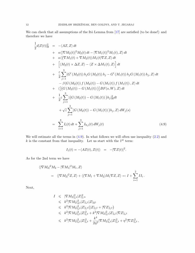
We will estimate all the terms in (4.9). In what follows we will often use inequality (2.2) andk is the constant from that inequality. Let us start with the 1st term:

I1(t) = −〈AZ(t), Z(t)〉 = −|∇Z(t)|2.

As for the 2nd term we have

〈|∇M2|2M2 − |∇M1|2M1, Z〉

= 〈|∇M2|2Z,Z〉+ 〈(∇M1 +∇M2)M1∇Z,Z〉 =: I +

2∑i=1

IIi .

Next,

I 6 |∇M2|2L2 |Z|2L∞

6 k2|∇M2|2L2 |Z|L2 |Z|H1

6 k2|∇M2|2L2 |Z|L2

(|Z|L2 + |∇Z|L2

)6 k2|∇M2|2L2 |Z|2L2 + k2|∇M2|2L2 |Z|L2 |∇Z|L2

6 k2|∇M2|2L2 |Z|2L2 +k4

2η2|∇M2|4L2 |Z|2L2 + η2|∇Z|2L2 ,

13

and

IIi 6 |∇Mi|L2 |M1|L∞ |∇Z|L2 |Z|L∞ 6 |∇Mi|L2 |∇Z|L2 |Z|L∞

6 k|∇Mi|L2 |∇Z|L2 |Z|12

L2

(|Z|

12

L2 + |∇Z|12

L2

)6 k|∇Mi|L2 |∇Z|L2 |Z|L2 + k|∇Mi|L2 |Z|

12

L2 |∇Z|32

L2

6k2

η2|∇Mi|2L2 |Z|2L2 + η2|∇Z|2L2 +

k4

4η6|∇Mi|4L2 |Z|2L2 +

3

4η2|∇Z|2L2 .

Hence,

I2(t) = 〈|∇M2|2M2 − |∇M1|2M1, Z〉 6 k2[|∇M2|2L2 +

k2

2η2|∇M2|4L2

+2∑i=1

1

η2|∇Mi|2L2 +

k2

4η6

2∑i=1

|∇Mi|4L2

]|Z|2L2 +

5

2η2|∇Z|2L2

Let us note now that by (2.7), the 2nd part of the 4th term, i.e. 〈Z × ∆M1, Z〉 is equalto 0. Next, by definition (2.5), similarly as the estimate of IIi above, we have the followingestimates for the 1st part of the 4th term using the bound |Z|L∞ 6 2, we get

〈M2 ×∆Z,Z〉 = −〈Z ×∇M2,∇Z〉 6 |Z|L∞ |∇M2|L2 |∇Z|L2

6k2

η2|∇Mi|2L2 |Z|2L2 + η2|∇Z|2L2 +

k4

4η6|∇Mi|4L2 |Z|2L2 +

3

4η2|∇Z|2L2

Therefore, we get the following inequality for the 4th term

I4(t) =[〈M2(t)×∆Z,Z〉 − 〈Z ×∆M1(t), Z〉

]6

k2

η2|∇Mi|2L2 |Z|2L2 + η2|∇Z|2L2 +

k4

4η6|∇Mi|4L2 |Z|2L2 +

3

4η2|∇Z|2L2

Next, we will deal with the 3rd term. Since |M1|L∞ = 1, the Holder inequality yields

〈∇MjM1∇Z,Z〉 6 |∇Mj |L2 |M1|L∞ |∇Z|L2 |Z|L∞ 6 ∇Mj |L2 |∇Z|L2 |Z|L∞

6k2

η2|∇Mi|2L2 |Z|2L2 + η2|∇Z|2L2 +

k4

4η6|∇Mi|4L2 |Z|2L2 +

3

4η2|∇Z|2L2 .

Therefore, we get the following inequality for the 3rd term

I3(t) = 〈(∇M1 +∇M2)M1∇Z,Z〉 =

2∑j=1

〈∇MjM1∇Z,Z〉 6k2

η2

( 2∑i=1

|∇Mi|2L2

)|Z|2L2

+ η2|∇Z|2L2 +k4

4η6

( 2∑i=1

|∇Mi|4L2

)|Z|2L2 +

3

2η2|∇Z|2L2

By inequalities (4.4), (4.6) and (4.7) we get the following bound for the 5th, 6th and 8th

terms ∑i=5,6,8

Ii(t) 6 C1|Z(t)|2L2 .


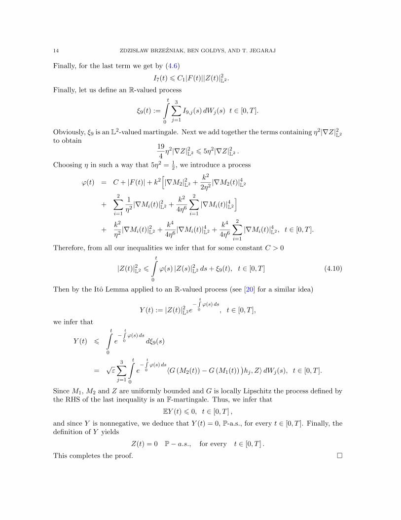
Finally, for the last term we get by (4.6)

I7(t) 6 C1|F (t)||Z(t)|2L2 .

Finally, let us define an R-valued process

ξ9(t) :=

t∫0

3∑j=1

I9,j(s) dWj(s) t ∈ [0, T ].

Obviously, ξ9 is an L2-valued martingale. Next we add together the terms containing η2|∇Z|2L2

to obtain19

4η2|∇Z|2L2 6 5η2|∇Z|2L2 .

Choosing η in such a way that 5η2 = 12 , we introduce a process

ϕ(t) = C + |F (t)|+ k2[|∇M2|2L2 +

k2

2η2|∇M2(t)|4L2

+2∑i=1

1

η2|∇Mi(t)|2L2 +

k2

4η6

2∑i=1

|∇Mi(t)|4L2

]+

k2

η2|∇Mi(t)|2L2 +

k4

4η6|∇Mi(t)|4L2 +

k4

4η6

2∑i=1

|∇Mi(t)|4L2 , t ∈ [0, T ].

Therefore, from all our inequalities we infer that for some constant C > 0

|Z(t)|2L2 6

t∫0

ϕ(s) |Z(s)|2L2 ds+ ξ9(t), t ∈ [0, T ] (4.10)

Then by the Ito Lemma applied to an R-valued process (see [20] for a similar idea)

Y (t) := |Z(t)|2L2e−

t∫0

ϕ(s) ds, t ∈ [0, T ],

we infer that

Y (t) 6

t∫0

e−

t∫0

ϕ(s) dsdξ9(s)

=√ε

3∑j=1

t∫0

e−

t∫0

ϕ(s) ds〈G (M2(t))−G (M1(t))

)hj , Z〉 dWj(s), t ∈ [0, T ].

Since M1, M2 and Z are uniformly bounded and G is locally Lipschitz the process defined bythe RHS of the last inequality is an F-martingale. Thus, we infer that

EY (t) 6 0, t ∈ [0, T ] ,

and since Y is nonnegative, we deduce that Y (t) = 0, P-a.s., for every t ∈ [0, T ]. Finally, thedefinition of Y yields

Z(t) = 0 P− a.s., for every t ∈ [0, T ] .

This completes the proof.

15

Remark 4.3. Our uniqueness result should also hold in a stronger sense as follows. Supposethat M1 is a solution in the sense of the last theorem and M2 a solution in the sense ofTheorem 3.1, defined on the same filtered probability space. Then M1 = M2 as in Theorem4.2.

By an infinite-dimensional version of the Yamada and Watanabe theorem [16] pathwiseuniqueness and the existence of weak solutions implies uniqueness in law and the existence ofa strong solution. In Theorem 4.4 below, we state such a result for equation (3.1). In whatfollows we say ‘weak solution’ instead of ‘weak martingale solution’ and, to simplify notation,we set

ST := C([0, T ];H) ∩ L4(0, T ;H1). (4.11)

Theorem 4.4. Let assumptions of Theorem 4.2 be satisfied. Then uniqueness in law and theexistence of a strong solution holds for equation (3.1) in the following sense:

(1) if (W,M) and (W ′,M ′) are two weak solutions of equation (3.1) with W and W ′ beingtwo Wiener processes, defined on possibly different probability spaces and M and M ′

are ST -valued random variables, then M and M ′ have the same law on ST ;(2) there exists a measurable function J :

(C([0, T ];R3

),BC([0,T ];R3)

)→ (ST ,BST ) with

the following property: for any filtered probability space (Ω, F , (Ft)t∈[0,T ], P), where

the filtration (Ft) is such that F0 contains all sets in F of P-measure zero, and

for any (Ft)-Wiener process (W (t))t∈[0,T ] defined on this space, the process J(W ) is

(Ft)-adapted and the pair (W , J(W )) is a weak solution of equation (3.1).

By Theorem 4.2 it is enough to apply in the space ST the Yamada-Wantanbe theorem in theversion proved in [16].

5. Further regularity

In this section, we assume that (W,M) is a given weak solution of equation (3.1) such thatM has paths in the space ST defined in (4.11). Recall that, by Theorem 4.4, the law of M isunique. Some regularity properties of M are listed in Theorem 3.1. The main result of thissection is Theorem 5.2, where we prove stronger regularity of the solution. In Proposition 5.4,we use this estimate to show that paths of M lie in C([0, T ];H1), P-almost everywhere; thisimproves upon the continuity property in Theorem 3.1.We start with a lemma that expresses M in a form which allows us to exploit the regularizingproperties of the semigroup (e−tA). The proof of this well known fact is omitted.

Lemma 5.1. For each t ∈ [0, T ] P-a.s.

M(t) = e−αtAM0 +

t∫0

e−α(t−s)A(M ×∆M)ds+ α

t∫0

e−α(t−s)A (|∇M |2M) ds+

t∫0

e−α(t−s)AG(M)BF (s,W ) ds+ ε12

t∫0

e−α(t−s)AG(M)B dW (s)

− βt∫

0

e−α(t−s)Af(M) ds+ε

2

3∑i=1

t∫0

e−α(t−s)AG′(M)hiG(M)hi ds.

(5.1)


Theorem 5.2. Assume that M0 ∈ H1, F ∈ PT and h =(hi)3i=1∈ (H1)3 and let M be the

corresponding weak solution. Then there exists a constant C = C (α, T, ‖F‖, ‖M0‖, |h|) suchthat

E

T∫0

|∆M(t)|2H dt+

T∫0

|∇M(t)|4L4 dt

6 C.Proof. We will use repeatedly the following well known properties of the semigroup

(e−tA

).

The semigroup(e−tA

), where A is defined in 2.1, is ultracontractive (see, for example, [2]),

that is, there exists C > 0 such that for 1 6 p 6 q 6∞

|e−tAf |Lq 6C

t12

(1p− 1q

) |f |Lp , f ∈ Lp, t > 0. (5.2)

It is also well known that A has maximal regularity property, that is, there exists C > 0 suchthat for any f ∈ L2 (0, T ;H) and

u(t) =

t∫0

e−(t−s)Af(s)ds, t ∈ [0, T ],

we haveT∫

0

|Au(t)|2H dt 6 C

T∫0

|f(t)|2H dt. (5.3)

Without loss of generality we may assume that h2 = h3 = 0 and put h1 = h. Then by Lemma5.1 M can be written as a sum of seven terms:

M(t) =

6∑i=0

mi(t),

and we will consider each term separately. Let us fix for the rest of the proof T > 0 andδ ∈

(58 ,

34

). In what follows, C stands for a generic constant that depends on T only. In order

to simplify notation, we put (without loss of generality) ε = α = 1.We will show first that

ET∫

0

|M(t)|4W1,4 dt 6 C (α, T,R,M0, h) . (5.4)

To this end we will prove a stronger estimate:

ET∫

0

∣∣∣AδM(t)∣∣∣4Hdt 6 C (α, T,R,M0, h) . (5.5)

Then (5.4) will follow from the Sobolev imbedding Xδ →W1,4.We start with m0. For each t ∈ (0, T ], we have∣∣∣Aδe−tAM0

∣∣∣4H6

C

t4δ−2|M0|4H1 ,

17

and therefore,T∫

0

∣∣∣Aδm0(t)∣∣∣4Hdt 6 C |M0|4H1 . (5.6)

We will consider m1. Putting f = M ×∆M we have

|Aδe−(t−s)Af(s)|H 6 C(t− s)−δ|f(s)|H, 0 < s < t < T,

hence applying the Young inequality we obtain

T∫0

|Aδm1(t)|4H dt 6 C

T∫0

t∫0

(t− s)−δ|f(s)|H ds

4

dt

6 C

T∫0

s−4δ/3 ds

3 T∫0

|f(s)|2H ds

2

.

Thereby, since 43δ < 1, part (3) of Theorem 3.1 yields

ET∫

0

|Aδm1(t)|4H dt 6 C(R, T,M0, h). (5.7)

Since for every t ∈ [0, T ] we have |M(t, x)| = 1- x-a.e. and h ∈ H1, the estimate (??) impliesthat there exists deterministic c > 0 such that

|G(M)|+ |G′(M)hG(M)h| 6 c.

Therefore, the same arguments as for m1 yield

ET∫

0

|Aδm3(t)|4H dt 6 C(R, T,M0, h). (5.8)

and

ET∫

0

|Aδm5(t)|4H dt 6 C(R, T,M0, h). (5.9)

We will consider the next term m2 using the fact that f = |∇M |2M ∈ L1(0, T ;H). Invokingthe semigroup property of e−tA and the ultracontractive estimate (5.2) with p = 1 and q = 2we find that there exists C > 0 such that obtain for s, t such that P-a.s.

|Aδe−(t−s)Af(s)|H 6C

(t− s)δ+14

supr6T|M (r) |2H1 , 0 < s < t ∈ [0, T ].

Therefore,

T∫0

∣∣∣∣∣∣t∫

0

Aδe−(t−s)Af(s) ds

∣∣∣∣∣∣4

H

dt 6 C supr6T|M (r) |8H1

T∫0

t∫0

ds

(t− s)δ+14

ds

4

dt


hence (since δ + 14 < 1) Theorem 3.1 yields

ET∫

0

∣∣∣Aδm2(t)∣∣∣4Hdt 6 C (R, T,M0, h) . (5.10)

In order to estimate m4 we recall that

|∇G(M(s))h| 6 a+ b|∇M(s)|, (5.11)

where a, b > 0 are constants depending on h only. Invoking Lemma 7.2 in [9] we find that forany t ∈ [0, T ]

E

∣∣∣∣∣∣t∫

0

Aδe−(t−s)AG(M(s))h dW (s)

∣∣∣∣∣∣4

H

6 C(T )E

t∫0

|Aδe−α(t−s)AG(M(s))h|2H ds

2

= C(T )E

t∫0

|Aδ−12 e−(t−s)AA

12G(M(s))h|2H ds

2

6 C(T )E

t∫0

|G(M(s))h|2H1

(t− s)2δ−1ds

2

6 C(T )E supr6T|M (r) |8H1 .

Theorem 3.1 now yields

ET∫

0

|Aδm4(t)|4H dt 6 C(T,R,M0, h). (5.12)

Finally, combining estimates (5.6) to (5.12) we obtain (5.5) and (5.4) follows.It remains to prove that

ET∫

0

|AM(t)|2H dt 6 C(T,R,M0, h). (5.13)

To this end we note first that using the maximal inequality (5.13) and the first part of theproof it is easy to see that

ET∫

0

|Ami(t)|2H dt 6 C(T,R,M0, h), i = 1, 2, 3, 5. (5.14)

The estimateT∫

0

|Am0(t)|2H dt 6 C (M0) , (5.15)

19

is an immediate consequence of the fact that M0 ∈ H1 = D(A1/2

).

We will consider now the stochastic term m4. Using (5.11), a result of Pardoux in [17] andpart 1 of Theorem 3.1 we find that

ET∫

0

|Am4(t)|2Hdt 6 ET∫

0

(a|∇(M(t))|2H + b

)dt

6 C (α, T,R,M0, h) .

(5.16)

Combining (5.14), (5.15) and (5.16) we obtain (5.13) and the proof is complete.

Remark 5.3. By estimate (5.4) the vector AM(t, x) ∈ R3 is well defined t, x-a.e. and|M(t, x)|2 = 1 t, x-a.e., hence

M(t, x) ·∆M(t, x) = −|∇M(t, x)|2, t, x− a.e.

Therefore, an elementary identity

|a× b|+ |a · b|2 = |a|2 · |b|2, a, b ∈ R3,

yields

|M(t, x)×∆M(t, x)|2 + |∇M(t, x)|4 = |∆M(t, x)|2, t, x− a.e.

Proposition 5.4. Paths of M lie in C([0, T ];H1), P-a.s.

Proof. The proposition follows easily from the results in [17].

Corollary 5.5. Let hi ∈W1,3, i = 1, 2, 3, and let F ∈PT . Let W be an FT -adapted Wienerprocess probability space (Ω,F ,FT ,P) Then, for every M0 ∈ H1 and ε > 0, there exists aunique pathwise solution M ε ∈ C

([0, T ];H1

)∩ L2 (0, T ;D(A)) of the equation

M(t) = M0 + α

t∫0

∆M ds+ α

t∫0

|∇M |2M ds+

t∫0

M ×∆M ds

ε

2

3∑i=1

t∫0

G′(M)hiG(M)hi ds+√ε

t∫0

G(M) dW (s)

− βt∫

0

G(M)f(M) ds+

t∫0

G(M)F (s,W ) ds,

where all the integrals,except the Ito integral, are the Bochner integrals in H.

In what follows we will denote by XT the Banach space

XT = C([0, T ];H1

)∩ L2(0, T ;D(A)).

6. Small noise asymptotics

In this section we will prove the large deviation principle for the family of laws of thesolutions of equation (3.1) with F identically zero and the parameter ε ∈ (0, 1] approachingzero.


The setting in this section is given by a probability space (Ω,F ,P) carrying an R3-valuedWiener process (W (t))t∈[0,T ]. We will denote by

(F 0t

)the natural filtration of this Wiener

process. For each ε ∈ [0, 1] and F ∈PT , let

JεF : C([0, T ];R3

)→ S

denote the Borel mapping defined in Theorem 4.4 that acts on a Wiener process to give aweak solution of equation (3.1). By Corollary 5.5 the image of the Wiener process under themap JεF has paths in XT almost surely. In what follows, we consider JεF as a Borel map

JεF : C([0, T ];R3

)→XT .

If F (t,W ) = v(t) with v ∈ L2(0, T ;R3

)is deterministic, then by Corollary 5.5 the function

yv = J0v is the unique solution of the equation

yv(t) = M0 + α

t∫0

∆yv ds+ α

t∫0

|∇yv|2 yv ds+

t∫0

yv ×∆yv ds (6.1)

− βt∫

0

G (yv) f (yv) ds+

t∫0

G (yv)Bv(s) ds,

where the mapping G has been defined in (2.11) and hi ∈W1,3 for i = 1, 2, 3. Hence the map

L2(0, T ;R3

)3 v −→ J0

v ∈XT

is well defined. We will define now the rate function I : XT → [0,∞] by the formula

I(u) := inf

1

2

T∫0

|φ(s)|2 ds : φ ∈ L2(0, T ;R3

)and u = J0

φ

where the infimum of the empty set is taken to be infinity.For R > 0, define

BR :=

φ ∈ L2(0, T ;R3

):

T∫0

|φ(s)|2 ds 6 R2

with the weak topology of L2(0, T ;R3

).

In order to show that the family of laws L (Jε0(W )) : ε ∈ (0, 1] satisfies the large deviationprinciple with the rate function I we will follow the weak convergence method of Budhirajaand Dupuis [5], see also Duan and Millet [10] and Chueshov and Millet [7]. To this end weneed to show that the following two statements are true.

Statement 1. For each R > 0, the setJ0v : v ∈ BR

is a compact subset of XT .

Statement 2. Let (εn) be any sequence from (0, 1] convergent to 0 and let (vn) be anysequence of R-valued

(F 0t

)-predictable processes defined on [0, T ] such that ‖v‖T 6 R for a

certain R > 0. Then if (vn) converges in law on BR to v, then (Jεnvn (W ) converges in law on

XT to J0v .

The remaining part of this section is devoted to the proof of thsese two statements.

21

Lemma 6.1. Suppose that (wn) ⊂ L2(0, T ;R3

)is a sequence converging weakly to w. Then

the sequence ywn converges strongly to yw in XT . In particular, the mapping

BR 3 w −→ J0w ∈XT

is Borel.

Proof of Lemma 6.1. To simplify notation, we write yn for ywn , y for yw and set un = yn− y.Let

R2 = supn∈N

T∫0

|wn|2 (s) ds.

Let us recall the notation h = (hi). By Theorem 3.1, Theorem 5.2 and uniqueness of solutions,there exists a finite constant C (T, α,R,M0, h) such that for all n ∈ N:

supt∈[0,T ]

|yn(t)|H1 6 C(T, α,R,M0, h), (6.2)

T∫0

(|∆yn(s)|2H + |∇yn|4L4

)ds 6 C(T, α,R,M0, h) (6.3)

and clearly

|yn(t)(x)| = 1, x ∈ Λ, t ∈ [0, T ]. (6.4)

The same estimates hold for y.

Step 1. We note first that each subsequence of (yn) has a further subsequence that convergesin C([0, T ];H) strongly. Indeed, since H1 is compactly embedded in H, the estimate (6.2)implies that for each fixed t ∈ [0, T ], yn(t) : n > 1 is relatively compact in H. Hence, itis enough to show that yn : n > 1 is a uniformly equicontinuous subset of C([0, T ];H). Tothis end we write for 0 6 t < t′ 6 T :

yn(t′)− yn(t) =

t′∫t

yn ×∆yn ds+ α

t′∫t

∆yn ds+ α

t′∫t

|∇yn|2 yn ds

− βt′∫t

G (yn) f (yn) ds+

t′∫t

G (yn)Bwn ds.

Then (6.2), (6.3) and the Cauchy-Schwarz inequality yield immediately

|yn(t′)− yn(t)|H 6 (1 + α)(√

C(T, α,R,M0, h) +R|M0|H|h|L∞

)√t′ − t.

This completes the proof of Step 1.

Step 2. Let q ∈ L2(0, T ;H). Recall that wn → w weakly in L2(0, T ;R3

). We will show that

limn→∞

supt∈[0,T ]

∣∣∣∣∣∣t∫

0

〈q(s), un(s)〉H(wn(s)− w(s)) ds

∣∣∣∣∣∣ = 0. (6.5)


By Step 1 we can assume that un → u∞ in C([0, T ];H). For n ∈ N∪∞ we define operatorsKn : L2

(0, T ;R3

)→ C

([0, T ];R3

)by the formula

Knv(t) =

t∫0

〈q(s), un(s)〉H v(s) ds, t ∈ [0, T ], v ∈ L2(0, T ;R3

).

The operators Kn, are compact because the functions 〈q(·), un(·)〉H belong to L2 (0, T ;R).Moreover, since the sequence 〈q(·), un(·)〉H converges strongly in L2 (0, T ;R) to a function〈q(·), u∞(·)〉H we infer that

limn→∞

‖Kn −K∞‖ = 0.

Since

|Kn (wn − w)|C([0,T ];R3)) 6 ‖Kn −K∞‖ · |wn − w|L2([0,T ];R3) + |K∞ (wn − w)|C([0,T ];R3) ,

the claim follows immediately by the compactness ofK∞ because wn → w weakly in L2([0, T ];R3

).

Step 3. We will establish uniform estimates on un. More precisely, we will show that

supn∈N

[supt∈[0,T ]

|un(t)|2H1 + α

T∫0

|∆un|2H ds]<∞. (6.6)

Without loss of generality we may assume that h2 = h3 = 0 and put h1 = h and w1n = wn ∈ R.

For each n > 1, we have

un(t) =

t∫0

un ×∆yn ds+

t∫0

y ×∆un ds

+ α

t∫0

(|∇yn| − |∇y|)(|∇yn|+ |∇y|)yn ds

+ α

t∫0

|∇y|2un ds+ α

t∫0

∆un ds

− βt∫

0

G (yn) f (un) ds− βt∫

0

(G (yn)−G(y)) f(y) ds

+

t∫0

(un × h)wn ds+

t∫0

G(y)h(wn − w) ds

− α

t∫0

un × (yn × h)wn ds+

t∫0

y × (un × h)wn ds

.

(6.7)

Note that each integrand on the right hand side of (6.7) is square integrable in H, because of(6.2), (6.3) and (6.4). Therefore,

d

dt|un(t)|2H1 = 2

⟨d

dtun(t), (I +A)un(t)

⟩H, t ∈ [0, T ]. (6.8)

23

Let N be an arbitrary positive integer. The functions s 7→ y(s), s 7→ y(s) × πNh ands 7→ y(s)× (y(s)× πNh) all belong to L2(0, T ;D(A)). Therefore, from (6.8) we have:

1

2

d

dt|un(t)|2H1 = 〈un ×∆yn,−∆un〉H + 〈y(s)×∆un, un〉H

+ α〈(|∇yn| − |∇y|)(|∇yn|+ |∇y|)yn, un −∆un〉H+ α〈|∇y|2un, un −∆un〉H ds− α|∇un|2H − α|∆un|2H− β 〈G (yn) f (un) , un −∆un〉H − β 〈(G (yn)−G(y)) f(y), un −∆un〉H(6.9)

− 〈un × h,∆un〉Hwn + 〈G(y)h, un〉H(wn − w)

− 〈∆(y × πNh), un〉H(wn − w)− 〈y × (h− πNh),∆un〉H(wn − w)

+ α〈un × (yn × h),∆un〉Hwn − α〈y × (un × h), un −∆un〉Hwn ds+ α〈∆(y × (y × πNh)), un〉H(wn − w)

+ α〈y × (y × (h− πNh)),∆un〉H(wn − w) (6.10)

for all t ∈ [0, T ]. In the rest of this proof, C and C1 denote positive real constants whose valuemay depend only on α, T , R, M0 and h; the actual value of the constant may be differentin different instances. For each η > 0 we estimate the terms on the right hand side of (6.10)using the Cauchy-Schwarz inequality and (2.2) and the Young inequality to obtain:

|un(t)|2H1 + 2α

t∫0

|∆un|2H ds 6 C1η2

t∫0

|∆un|2H ds+ bn,N + C

t∫0

|un|2H1ψn(s) ds

+ C|h− πNh|H

T∫0

|∆un(s)|2H ds

12 T∫

0

(wn(s)− w(s))2 ds

12

(6.11)

where, for s ∈ [0, T ], we put1

ψn(s) = 1 +1

η2+

1

η2|∆yn(s)|2H

+

(1 +

1

η2

)[|yn(s)|H1 (|yn(s)|H1 + |∆yn(s)|H)

+ |y(s)|H1(|y(s)|H1 + |∆y(s)|H)

+|y(s)|2H1

(|y(s)|2H1 + |∆y(s)|2H

)]+

1

η2w2n + |wn(s)|

1Note that the functions yn satisfy the uniform estimates (6.3) and so

supn

∫ T

0

ψn(s) ds <∞.

.


and

bn,N = supr6T

∣∣∣∣∣∣r∫

0

〈G(y(s))h(s), un〉H(wn(s)− w(s)) ds

∣∣∣∣∣∣+ sup

r6T

∣∣∣∣∣∣r∫

0

〈∆(y(s)× πNh(s)), un(s)〉H(wn(s)− w(s)) ds

∣∣∣∣∣∣+ C sup

r6T

∣∣∣∣∣∣r∫

0

〈∆(y(s)× (y(s)× πNh(s))), un(s)〉H(wn(s)− w(s)) ds

∣∣∣∣∣∣+ C

T∫0

|un(s)|2H ds.

We choose η > 0 such that C1η2 = α

2 in (6.11) and use the boundedness of the sequence wnin L2

(0, T ;R3

)together with the Holder inequality to estimate the product of square roots

in the second line of (6.11) to obtain

|un(t)|2H1 + α

t∫0

|∆un(s)|2H ds 6 Ct∫

0

ψn(s)|un(s)|2H1 ds+ bn,N . (6.12)

By estimates (6.2) and (6.3)

γ := supn>1

T∫0

ψn(s) ds <∞

and γ depends on α, T , R, M0 and h only. Applying the Gronwall lemma we obtain

supt∈[0,T ]

|un(t)|2H1 + α

T∫0

|∆un|2H ds 6 bn,NeγT (6.13)

what completes the proof of estimates (6.13). Therefore, since by Claim(6.5) bn,N → 0 asN →∞ we infer that

lim supn→∞

supt∈[0,T ]

|un(t)|2H1 + α

T∫0

|∆un|2H ds

6 C |h− πNh|2H . (6.14)

We complete the proof of Lemma 6.1 by taking the limit as N →∞.

Note, that Statement 1 follows Lemma 6.1.

Now we will occupy ourselves with the proof of that Statement 2. For this purpose let uschhose and fix the following processes:

Yn = J εnvn and yn = J0vn .

Let N > |M0|H1 be fixed. For each n > 1 we define an (Ft)-stopping time

τn = inf t > 0 : |Yn(t)|H1 > N ∧ T. (6.15)

25

Lemma 6.2. For τn as defined in (6.15) we have

limn→∞

E

supt∈[0,T ]

|Yn (t ∧ τn)− yn (t ∧ τn)|2H +

τN∫0

|Yn − yn|2H1 ds

= 0.

Proof. Let Xn = Yn − yn. We assume without loss of generality that β = 0, h2 = h3 = 0 andh1 = h. Then for any n > 1 we have

dXn = α∆Xndt

+ α (∇Xn) · (∇ (Yn + yn))Yndt+ α |∇yn|2Xndt

+Xn ×∆Yndt+ yn ×∆Xndt

+ (G (Yn)−G (yn))hvndt

+√εnG (Yn)hdW +

εn2G′ (Yn)G (Yn)hdt

(6.16)

Using a version of the Ito formula given in [17] and integration by parts we obtain

1

2d |Xn|2H = −α |Xn|2H1 dt+ α ||∇yn|Xn|2H dt

+ α 〈Xn, (∇Xn) · (∇ (Yn + yn))Yn〉H dt− 〈∇Xn, Xn ×∇yn〉H dt+ 〈(G (Yn)−G (yn))h,Xn〉H vndt

+εn2zndt+

√εn 〈G (Yn)h,Xn〉H dW

where zn is a process defined by

zn =⟨G′ (Yn)G (Yn)h,Xn

⟩H + |G (Yn)h|2H .

Therefore

|Xn(t)|2H + 2α

t∫0

|Xn|2H1 ds 6 C

t∫0

|Xn|H |Xn|H1 |yn|2H1 ds

+ C

t∫0

|Xn|3/2H1 |Xn|H (|yn|H1 + |yn|H1) ds

+ C

t∫0

|Xn|3/2H1 |Xn|H |yn|H1 ds

+ C

t∫0

|Xn|2H |vn| ds

+ Cεn +√εn

∣∣∣∣∣∣t∫

0

〈G (Yn)h,Xn〉H dW

∣∣∣∣∣∣ .


By (6.2) we have supn |yn|H1 < ∞ and therefore, using repeatedly the Young inequality wefind that there exists C > 0 such that for all t ∈ [0, T ]

|Xn(t)|2H + α

t∫0

|Xn|2H1 ds 6 C

t∫0

|Xn|2H(

1 + |vn|+ β |yn|4H1

)ds

+ Cεn +√εn

∣∣∣∣∣∣t∫

0


∣∣∣∣∣∣ .Denoting the left hand side of the above inequality by Lt and using the definition of τn wehave

Lt∧τn 6 C

t∧τn∫0

|Xn|2H(

1 + |vn|+ β |yn|4H1

)ds

+ Cεn +√εn

∣∣∣∣∣∣t∧τn∫0


∣∣∣∣∣∣6

t∧τn∫0

|Xn|2H ψn,Nds+ Cεn

+√εn

∣∣∣∣∣∣t∧τn∫0


∣∣∣∣∣∣ ,where

ψn,N (s) = 1 + |vn(s)|+ βN4, s 6 T.

Since

supn

supt∈[0,T ]

〈G (Yn(t)) , Xn(t)〉2 6 C, P− a.s.,

the Burkoholder-Davis-Gundy inequality yields

E sups6t

Ls∧τn 6 C√εn +

t∫0

E supr6s|Xn (r ∧ τn)|2H ψn,Nds, (6.17)

and therefore

E supr6t|Xn(r ∧ τn)|2H 6 C

√εn +

t∫0

E supr6s|Xn (r ∧ τn)|2H ψn,Nds.

Clearly,

supn>1

T∫0

ψn,Nds <∞,

27

hence the Gronwall Lemma implies

E supr6T|Xn(r ∧ τn)|2H 6 C

√εne

T∫0

ψn,Nds→ 0 as n→∞.

Returning now to (6.17), we also have

Eτn∫

0

|Xn(s)|2H1 ds 6 C√εne

T∫0

ψn,Nds→ 0 as n→∞.

This completes the proof of Lemma 6.2.

Lemma 6.3. For the stopping time τn defined in (6.15) we have

limn→∞

E

supt∈[0,T ]

|∇(Yn(t ∧ τn)− yn(t ∧ τn))|2H +

τn∫0

|∆(Yn − yn)|2H ds

= 0.

Proof. By a version of the Ito formula, see [17],

1

2d|∇(Yn(t)− yn(t))|2H = −〈∆ (Yn − yn) , d (Yn − yn)〉H + εn |∇G (Yn)h|2H dt.

Therefore, putting Xn = Yn − yn and invoking equality (6.16) we obtain for any η > 0

1

2d |∇Xn(t)|2H = −α |∆Xn|2H

− α 〈∆Xn,∇Xn · (∇Yn +∇yn)Yn〉H dt

− α⟨

∆Xn, |∇yn|2Xn

⟩Hdt

− 〈Xn ×∆yn,∆Xn〉H dt− 〈(G (Yn)−G (yn))h,∆Xn〉H Fndt−√εn 〈∇G (Yn)h,∆Xn〉H dW

− εn2

⟨G′ (Yn)G (Yn)h,∆Xn

⟩H dt

+ εn |∇G (Yn)h|2H dt.

(6.18)

We will estimate the terms in (6.18). First, noting that

〈Xn ×∆Yn,∆Xn〉H = 〈Xn ×∆un,∆Xn〉H

we find that

|〈Xn ×∆Yn,∆Xn〉H| 6 Cη2 |∆Xn|2H +

C

η2|Xn|H |Xn|H1 . (6.19)


Next, by the Young inequality and the interpolation inequality (2.2)

|〈∆Xn,∇Xn · (∇Yn +∇yn)Yn〉H| 6 Cη2 |∆Xn|2H

+C

η2

∫Λ

|∇Xn|2(|∇Yn|2 + |∇yn|2

)dx

6 Cη2 |∆Xn|2H

+C

η2|∇Xn|2∞

∫Λ

(|∇Yn|2 + |∇yn|2

)dx

6 Cη2 |∆Xn|2H

+C

η2|Xn|H1 (|Xn|H1 + |∆Xn|H)

(|Yn|2H1 + |yn|2H1

)

,

and thereby

|〈∆Xn,∇Xn · (∇Yn +∇yn)Yn〉H| 6 Cη2 |∆Xn|2H

+C

η2|Xn|2H1

(|Yn|2H1 + |yn|2H1

)+C

η6|Xn|2H1

(|Yn|4H1 + |yn|4H1

)6 Cη2 |∆Xn|2H + Cη |Xn|2H1

(1 + |Yn|4H1

).

(6.20)

Finally, using (2.2) we obtain

|⟨

∆Xn, |∇yn|2Xn

⟩H| 6 |∆Xn|H |∇yn|L∞ |∇yn|H |Xn|L∞

6 Cη2 |∆Xn|2H

+C

η2|yn|H1 (|yn|H1 + |∆yn|H) |yn|2H1 |Xn|H |Xn|H1 .

(6.21)

29

Taking into account (6.19), (6.20) and (6.21) we obtain from (6.18)

|∇Xn(t)|2H + 2α

t∫0

|∆Xn|2H ds 6 Cη2

t∫0

|∆Xn|2H ds

+ Cη supr6t

(1 + |Yn|4H1

) t∫0

|Xn|2H1 ds

+ Cη2

t∫0

|∆Xn|2H ds+ Cη

(supr6t|Xn(r)|H

)(supr6t|Xn(r)|H1

)

+ Cη2

t∫0

|∆Xn|2H ds+ Cη

(supr6t|Xn(r)|H

)(supr6t|Xn(r)|H1

)

+ Cη2

t∫0

|∆Xn|2H ds+ Cη supr6t|Xn(r)|2H

+√εn

∣∣∣∣∣∣t∫

0

〈∇G (Yn)h,∆Xn〉H dW

∣∣∣∣∣∣+ Cεn

t∫0

(1 + |∆Xn|2H

)ds.

(6.22)Choosing η in such a way that 4Cη2 = α we obtain

E

supt∈[0,T ]

|∇Xn (t ∧ τn) |2H + α

t∧τn∫0

|∆Xn|2H ds

6 Cη (1 +N4)E

τn∫0

|Xn|2H1 ds

+ Cη (1 +N)E supt∈[0,T ]

|Xn (t ∧ τn)|H

+√εnE sup

t∈[0,T ]

∣∣∣∣∣∣t∧τn∫0

〈∇G (Yn)h,∆Xn〉H dW

∣∣∣∣∣∣+ CεnE

T∫0

(1 + |∆Xn|2H

)ds.

By Theorem 5.2 there exists a finite constant C, depending on T , α, R, M0 and h only, suchthat for each n > 1

ET∫

0

|∆Yn(s)|2H ds 6 C(T, α,M, u0, h),


hence invoking the Burkholder-Davis-Gundy inequality we find that

E

supt∈[0,T ]

|∇Xn (t ∧ τn) |2H + α

t∧τn∫0

|∆Xn|2H ds

6 Cη (1 +N4)E

τn∫0

|Xn|2H1 ds

+ Cη (1 +N)E supt∈[0,T ]

|Xn (t ∧ τn)|H

+ C(1 +N)√εn.

Finally, Lemma 6.3 follows from Lemma 6.2.

Lemma 6.4. Let (εn) ⊂ (0, 1] with εn → 0 and let (Fn) ⊂PT be such a sequence that

supn>1‖Fn‖T 6 R, for every ω ∈ Ω,

and Fn converges to F in law on BR. Then the sequence of XT -valued random elements(JεnFn(W )− J0

Fn) converges in probability to 0.

Proof. We will use the same notation as in the proof of Lemma (6.3). Let δ > 0 and ν > 0.Invoking part (2) of Theorem (3.1) we can find N > |M0|H1 such that

1

Nsupn>1

E supt∈[0,T ]

|Yn(t)|H1 <ν

2.

Then invoking Lemma 6.3 we find that for all n sufficiently large

P

supt∈[0,T ]

|Yn(t)− un(t)|2H1 +

T∫0

|Yn − un|2D(A) ds > δ

6 P

supt∈[0,T ]

|Yn(t ∧ τn)− un(t ∧ τn)|2H1 +

τn∫0

|Yn − un|2D(A) ds > δ, τn = T

+ P

(supt∈[0,T ]

|Yn(t)|H1 > N

)

61

δE

supt∈[0,T ]

|Yn(t ∧ τn)− un(t ∧ τn)|2H1 +

τn∫0

|Yn − un|2D(A) ds

+

1

NE supt∈[0,T ]

|Yn(t)|H1

< ν.

Theorem 6.5. The family of laws L (Jε0(W )) : ε ∈ (0, 1] on XT satisfies the large deviationprinciple with rate function I.

Proof. We interpret each process JεnFn(W ) as the solution of equation (3.1) with εn and Fn in

place of ε and F . In order to use Theorem 4.4 we note that any(F 0t

)-predictable process

31

u : [0, T ]× Ω→ R such that

T∫0

u2(t, ω) dt 6 R2, for all ω ∈ Ω

can be written as

u(t, ω) = F (t,W (ω)) ∀(t, ω) ∈ [0, T ]× Ω, (6.23)

for some (H 0t )-predictable function F : [0, T ]× C0([0, T ]) → R satisfying

T∫0

F 2(s, z) ds 6 R2

∀z ∈ C0([0, T ]). Statement 1 follows from Lemma 6.1.Next, we will show that Statement 2 holds true. Let (εn) be a sequence from (0, 1] thatconverges to 0 and let (Fn : [0, T ] × Ω → R) be a sequence of

(F 0t

)-predictable processes

that converges in law on BR, for some R > 0, to F . By Lemma 6.4 JεnFn(W )− J0Fn

converges

in probability (as a sequence of random variables in XT ) to 0. Lemma 6.1 implies that J0Fn

converges in distribution on XT to J0F . Indeed, since BR is a separable metric space, the

Skorohod Theorem (see, for example, [12, Theorem 4.30]) allows us to work with a sequenceof processes that converges in BR almost surely. These two convergence results imply that(JεnFn(W )

)converges in law on XT to J0

F . Thus, for any uniformly continuous and boundedfunction f : XT → R we have∣∣∣∣∣∣∣

∫Ω

f(JεnFn (W )

)dP−

∫XT

f(x) dL (J0F )(x)

∣∣∣∣∣∣∣6

∫Ω

|f(JεnFn(W ))− f(J0Fn)| dP

+

∣∣∣∣∣∣∣∫

XT

f(x) dL (J0Fn)(x)−

∫XT

f(x) dL (J0F )(x)

∣∣∣∣∣∣∣→ 0 as n→∞.

Therefore, Statement 2 is true as well and thus we conclude the proof of Theorem 6.5.

7. Application to a model of a ferromagnetic needle

In this section we will use the large deviation principle established in the previous section toinvestigate the dynamics of a stochastic Landau-Lifshitz model of magnetization in a needle-shaped particle. Here the shape anisotropy energy is crucial. When there is no applied fieldand no noise in the field, the shape anisotropy energy gives rise to two locally stable stationarystates of opposite magnetization. We add a small noise term to the field and use the largedeviation principle to show that noise induced magnetization reversal occurs and to quantifythe effect of material parameters on sensitivity to noise.

The axis of the needle is represented by the interval Λ and at each x ∈ Λ the magnetizationu(x) ∈ S2 is assumed to be constant over the cross-section of the needle. We define the total


magnetic energy of magnetization u ∈ H1 of the needle by

Et(u) =1

2

∫Λ

|∇u(x)|2 dx+ β

∫Λ

Φ(u(x)) dx−∫Λ

K (t, x) · u(x) dx, (7.1)

where

Φ(u) = Φ (u1, u2, u3) =1

2

(u2

2 + u23

),

β is the positive real shape anisotropy parameter and K is the externally applied magneticfield, such that K (t) ∈ H for each t.

With this magnetic energy, the deterministic Landau-Lifshitz equation becomes:

∂y

∂t(t) = y ×∆y − αy × (y ×∆y) +G(y) (−βf(y) + K (t)) (7.2)

where f(y) = ∇Φ(y), y ∈ R3. We assume, as before, that the initial state u0 ∈ H1 and|u0(x)|R3 = 1 for all x ∈ Λ. We also assume that the applied field K (t) : Λ→ R3 is constanton Λ at each time t. Equation (7.2) has nice features: the dynamics of the solution can bestudied using elementary techniques and, when the externally applied field K is zero, theequation has two stable stationary states, e1 = (1, 0, 0) and −e1.

We now outline the structure of this example. In Proposition 7.2, we show that if the appliedfield K is zero and the initial state u0 satisfies

|u0 ± e1|H1 <1

2k2√|Λ|

α

1 + 2α,

then the solution y(t) of (7.2) converges to ±e1 in H1 as t goes to ∞. In Lemma 7.3, weshow that if H = (H1,H2,H3)T ∈ R3 has norm exceeding a certain value (depending on

α and β) and the applied field is K = H + β|H |f(H ) and |u0 − H

|H | |H1 < 1k , then y(t)

converges in H1 to H|H | as t goes to ∞. Lemma 7.3 is used to show that, given δ ∈ (0,∞)

and T ∈ (0,∞), there is a piecewise constant (in time) externally applied field, K , whichdrives the magnetization from the initial state −e1 to the H1-ball centred at e1 and of radiusδ by time T ; in short, in the deterministic system, this applied field causes magnetizationreversal by time T (see Definition 7.4). What we are really interested in is the effect of addinga small noise term to the field. We will show that if K is zero but a noise term multipliedby√ε is added to the field, then the solution of the resulting stochastic equation exhibits

magnetization reversal by time T with positive probability for all sufficiently small positiveε. This result, in Proposition 7.5, is obtained using the lower bound of the large deviationprinciple. Finally, in Proposition 7.7, the upper bound of the large deviation principle isused: we obtain an exponential estimate of the probability that, in time interval [0, T ], thestochastic magnetization leaves a given H1-ball centred at the initial state −e1 and of radiusless than or equal to 1

2k2√|Λ|

α1+2α . This estimate emphasizes the importance of a large value

of β for reducing the disturbance in the magnetization caused by noise in the field.

7.1. Stable stationary states of the deterministic equation. In this subsection, weidentify stable stationary states of the deterministic equation (7.2) when the applied field Kdoes not vary with time.

33

Let ζ ∈ S2. Since the time derivative dydt of the solution y to (7.2), belongs to L2(0, T ;H) and

y belongs to L2(0, T ;D(A)), we have for all t > 0:

|y(t)− ζ|2H = |u0 − ζ|2H (7.3)

+ 2

t∫0

〈y − ζ, y ×∆y − αy × (y ×∆y)

+G(y)(−βf(y) + K 〉H ds

= |u0 − ζ|2H + 2

t∫0

〈−ζ, y ×∆y − αy × (y ×∆y)

+G(y)(−βf(y) + K 〉H ds

|∇y(t)|2H = |∇u0|2H − 2

t∫0

〈∆y,G(y) (−βf(y) + K ) (7.4)

− αy × (y ×∆y)〉H ds

Lemma 7.1. Let u ∈ H1 be such that u(x) ∈ S2 and

|u± e1|H1 61

2k2√|Λ|

α

1 + 2α.

Then for all x ∈ Λ

(1)1−u21(x)

u21(x)+ α

(1−u21(x))2

u21(x)− αu2

1(x) 6 0 for all x ∈ Λ,

(2) 〈u(x),±e1〉 > 34 and

(3) 78 |u(x)± e1|2 6 |u(x)× e1|2 .

Proof. By (2.2)

supx∈Λ|u(x)± e1|2 6 k2|u± e1|H|u− ζ|H1 ,

6 k2 2√|Λ| 1

2k2√|Λ|

α

1 + 2α=

α

1 + 2α. (7.5)

Invoking (7.5), we find that

u21(x) = 1− (u2

2(x) + u23(x)) > 1− |u(x)− ζ|2 > 1 + α

1 + 2α, x ∈ Λ. (7.6)

Hence one can use (7.6) and straightforward algebraic manipulations to verify that

1− u21(x)

u21(x)

+ α(1− u2

1(x))2

u21(x)

− αu21(x) 6 0.

Statements 2 and 3 of Lemma 7.1 follow easily from (7.5).

Proposition 7.2. Let the applied field K be zero and let u0 ∈ H1 satisfy

|u0 ± e1|H1 <1

2k2√|Λ|

α

1 + 2α. (7.7)

Let the process y be the solution to (7.2). Then y(t) converges to ±e1 in H1 as t→∞.


Proof. Using some algebraic manipulation and the fact that 〈∇y(s), y(s)〉 = 0 a.e. on Λ foreach s > 0, one may simplify equations (7.4) and (7.4).We obtain from (7.4):

|y(t)± e1|2H = |u0 ± e1|2H − 2α

t∫0

∫Λ

|∇y(s)|2〈y(s),±e1〉 dx ds

− 2αβ

t∫0

∫Λ

〈y(s),±e1〉|y(s)× e1|2 dx ds ∀t > 0, (7.8)

and

|∇y(t)|2H = |∇u0|2H − 2α

t∫0

|y(s)×∆y(s)|2H ds+ 2β

t∫0

∫Λ

R(s) dx ds ∀t > 0, (7.9)

where

R = ∇y1(y3∇y2 − y2∇y3) + α(∇y1)2 − αy21|∇y|2 (7.10)

=−y2∇y2 − y3∇y3

y1(y3∇y2 − y2∇y3)

+ α(1− y21)

(y2∇y2 + y3∇y3

y1

)2

− αy21((∇y2)2 + (∇y3)2.

Define

τ = inf

t > 0 : |y(t)± e1|H1 >

1

2k2√|Λ|

α

1 + 2α

.

Then, by our choice of u0, τ > 0. For each s ∈ [0, τ), y(s) satisfies the hypotheses ofLemma 7.1, hence and

y(s)(x) · (±e1) >3

4, x ∈ Λ,

|y(s)(x)× (±e1) |2 > 7

8|y(s)(x)± e1|2, x ∈ Λ.

and, invoking the Cauchy-Schwartz inequality

R 6

(1− y2

1

y21

+ α(1− y2

1)2

y21

− αy21

)((∇y2)2 + (∇y3)2) 6 0, x ∈ Λ. (7.11)

Consequently, from (7.8) and (7.9) we deduce that the functions |y(·)± e1|2H and |∇y(·)|2H arenonincreasing on [0, τ). Furthermore, we have

|y(t)± e1|2H 6 |u0 ± e1|2H −3

2α

t∫0

|∇y(s)|2H ds−21

16αβ

t∫0

|y(s)± e1|2H ds, t < τ, (7.12)

and|∇y(t)|2H 6 |∇u0|2H, t < τ. (7.13)

Suppose, to get a contradiction, that τ <∞. Then, from (7.12) and (7.13), we have

|y(τ)± e1|H1 6 |u0 ± e1|H1 <1

2k2√l(Λ)

α

1 + 2α,

35

which contradicts the definition of τ . Therefore, τ = ∞. Since (7.12) holds for all t > 0, wehave

∞∫0

|∇y(s)|2H ds+

∞∫0

|y(s)± e1|2H ds <∞.

Since both integrands are nonincreasing

limt→∞

(|∇y(t)|H + |y(t)± e1|H) = 0.

We will show next, that if the applied field has sufficiently large magnitude, then thereexists a stable stationary state that is roughly in the direction of the applied field.

Lemma 7.3. Assume that H ∈ S2 and a real number λ satisfies

λ >

(4β + 4αβ

3α∨ 2β + 4αβ − α

α

). (7.14)

Let the applied field be2

K := λH + βf(H ).

Let y be a solution to the problem (7.2) with initial data u0 satisfying |u0−H |H1 < 1k . Then

|y(t)−H |H1 6 |u0 −H |H1 e−12γt ∀t > 0, (7.15)

where

γ := (αλ+ α− 2β − 4αβ) ∧(

3

2αλ− 2β − 2αβ

)> 0

is positive, by condition (7.14).

Proof. We have, from (7.3) and (7.4) with ζ replaced by H :

|y(t)−H |2H (7.16)

= |u0 −H |2H − 2β

t∫0

〈y −H , y × f(y −H )〉H ds

− 2α

t∫0

∫Λ

|∇y|2(y ·H ) dx ds

− 2α

t∫0

|y ×H |2H ds

+ 2αβ

t∫0

〈y ×H , y × f(y −H )〉H ds ∀t > 0.

2Note that a constant function H is a stationary solution to the problem (7.2).


From (7.4) we have:

|∇y(t)|2H = |∇u0|2H + 2β

t∫0

〈∆y, y × f(y −H )〉H ds

− 2α

t∫0

|y ×∆y|2H ds

− 2α

t∫0

∫Λ

|∇y|2(y ·H ) dx ds

− 2αβ

t∫0

〈∆y, y × (y × f(y −H ))〉H ds ∀t > 0.

Define

τ1 := inft > 0 : |y(t)−H |H1 > 1k. (7.17)

By our choice of u0, τ1 is greater than zero. Observe that

supx∈Λ|y(t)(x)−H |R3 < 1 for all t < τ1. (7.18)

It is easy to check that for every t < τ1

3

4|y(t)−H |2H 6 |y(t)×H |2H 6 |y(t)−H |2H, (7.19)

and

y(t, x) ·H > 12 , x ∈ Λ. (7.20)

37

Adding equalities (7.16) and (7.17) we obtain for t > 0

|y(t)−H |2H1

= |u0 −H |2H1 − 4α

t∫0

∫Λ

|∇y|2 (y ·H ) dx ds

+ 2β

t∫0

〈∆y, y × f(y −H )〉H ds

− 2αβ

t∫0

〈∆y, y × (y × f(y −H ))〉H ds

− 2α

t∫0

|y ×H |2H ds

− 2β

t∫0

〈y −H , y × f(y −H )〉H ds

+ 2αβ

t∫0

〈y ×H , y × f(y −H )〉H ds

− 2α

t∫0

|y ×∆y|2H ds . (7.21)

Therefore for every t < τ1

|y(t)−H |2H1 6 |u0 −H |2H1 − (2α− 2β − 4αβ)

t∫0

|∇y|2H ds

− (32α− 2β − 2αβ)

t∫0

|y −H |2H ds

− 2α

t∫0

|y ×∆y|2H ds , (7.22)

where we used (7.18), (7.19) and (7.20). Because of hypothesis (7.14), the two expressions(2α− 2β − 4αβ) and (3

2α− 2β − 2αβ) on the right hand side of (7.22) are positive numbers.Suppose, to get a contradiction, that τ1 <∞. Then, from (7.22), we have

|y(τ1)−H |H1 6 |u0 −H |H1 < 1k ,


which contradicts the definition of τ1 in (7.17). Hence τ1 = ∞. It now follows from (7.22)that

∞∫0

|∇y(s)|2H ds < ∞, (7.23)

∞∫0

|y(s)−H |2H ds < ∞ (7.24)

and

∞∫0

|y(s)×∆y(s)|2H ds < ∞. (7.25)

From (7.21) and these three inequalities, the function t ∈ [0,∞) 7→ |y(t)−H |2H1 is absolutelycontinuous and, for almost every t > 0, its derivative is:

d

dt|y −H |2H1(t) = −4α

∫Λ

|∇y(t)|2(y(t) ·H ) dx

+ 2β〈∆y(t), y(t)× f(y −H )〉H− 2αβ〈∆y(t), y(t)× (y(t)× f(y −H ))〉H− 2α|y(t)×H |2H− 2β

⟨y(t)−H , y(t)× f(y −H )

⟩H

+ 2αβ〈y(t)×H , y(t)× f(y −H )〉H− 2α|y(t)×∆y(t)|2H

6 −(2α− 2β − 4αβ)|∇y(t)|2H− (3

2α− 2β − 2αβ)|y(t)−H |2H− 2α|y(t)×∆y(t)|2H

6 −γ|y(t)−H |2H1 , (7.26)

where

γ := (α+ αλ− 2β − 4αβ) ∧(

3

2αλ− 2β − 2αβ

)> 0.

Now the lemma follows by a standard argument.

7.2. Noise induced instability and magnetization reversal. In Proposition 7.2 weshowed that the states e1 and −e1 are stable stationary states of the deterministic Landau-Lifshitz equation (7.2) when the externally applied field K is zero. In this section we showthat a small noise term in the field may drive the magnetization from the initial state −e1 toany given H1-ball centred at e1 in any given time interval [0, T ]. We also find an exponentialupper bound for the probability that small noise in the field drives the magnetization outsidea given H1-ball centred at the initial state −e1 in time interval [0, T ]. Firstly we need adefinition.

Definition 7.4. Let δ be a given small positive real number. Suppose that the initial magne-tization is −e1 and that at some time T the magnetization lies in the open H1-ball centred ate1 and of radius δ. Then we say that magnetization reversal has occurred by time T .

39

We consider a stochastic equation for the magnetization, obtained by setting K to zero andadding a three dimensional noise term to the field. Denoting the magnetization by Y , theequation is:

dY = (Y ×∆Y − αY × (Y ×∆Y ) + βG(Y )f(Y )) dt

+√εG(Y )B dW (t)

Y (0) = −e1.

(7.27)

In (7.27), we assume that the vectors h1, h2, h3 ∈ R3 are linearly independent. The parameterε > 0 corresponds to the ‘dimensionless temperature’ parameter appearing in the stochasticdifferential equation (??) of Kohn, Reznikoff and Vanden-Eijnden []

Fix T > 0. There is no deterministic applied field in (7.27) but, as we will see, the lowerbound of the large deviation principle satisfied by the solutions Y ε (ε ∈ (0, 1)) of (7.27) impliesthat, for all sufficiently small positive ε, the probability of magnetization reversal by time Tis positive.

Firstly, we shall use Lemma 7.3 to construct a piecewise constant (in time) deterministicapplied field, K , such that the solution y of (7.2), with initial state (−1, 0, 0)T, undergoesmagnetization reversal by time T .Take points ui ∈ S2, i = 0, 1, . . . , N , such that u0 = −e1 and uN = e1 and

|ui − ui+1|H1 = |ui − ui+1|R3

√|Λ| < 1

kfor i = 0, 1, . . . , N − 1.

Let

η := min

1

k− |ui − ui+1|H1 : i = 1, . . . , N − 1

∧ δ

2.

Using Lemma 7.3, we can take the applied field to be

K (t) :=N−1∑i=0

1(i TN,(i+1) T

N](t)(Rui+1 + βf(ui+1)

), t > 0, (7.28)

with the positive real number R chosen to ensure that, as t varies from i TN to (i+ 1) TN , y(t)

starts at a distance of less than η from ui (i.e. |y(i TN ) − ui|H1 < η) and moves to a distance

of less than η from ui+1 (i.e. |y((i + 1) TN ) − ui+1|H1 < η). Specifically, we take R ∈ (0,∞)such that

1

ke−

12

[(αR+α−2β−4αβ)∧( 32αR−2β−2αβ)] T

N < η.

For each i = 0, 1, . . . , N − 1, let φi+1 = (φi+11 , φi+1

2 , φi+13 )T ∈ R3 be the vector of scalar

coefficients satisfying the equality

φi+11 a1 + φi+1

2 a2 + φi+13 a3 = Rui+1 + βf(ui+1),

and define

φ(t) :=

N−1∑i=0

1(i TN,(i+1) T

N](t) φ

i+1, t ∈ [0, T ]. (7.29)

We remark that the function φ depends on the chosen values of δ and T , the material param-eters Λ, α and β and the noise parameters a1, a2 and a3.


Recall that Y ε denotes the solution of (7.27). By an argument very much like that leadingto Theorem 6.5, the family of laws L (Y ε) : ε ∈ (0, 1) on XT satisfies a large deviationprinciple. In order to define the rate function, we introduce an equation

yψ(t) = −e1 +

t∫0

yψ ×∆yψ ds− αt∫

0

yψ × (yψ ×∆yψ) ds

− βt∫

0

G (yψ) f (yψ) ds+

t∫0

G (yψ)Bψ ds. (7.30)

By Corollary 5.5 this equation has unique solution yψ ∈XT for every ψ ∈ L2(0, T ;R3

). The

rate function I : XT → [0,∞], is defined by:

IT (v) := inf

1

2

T∫0

|ψ(s)|2 ds : ψ ∈ L2(0, T ;R3) and v = yψ

, (7.31)

where the infimum of the empty set is taken to be ∞.Let y be the solution of equation (7.2) with u0 = −e1 and K as defined in (7.28). Using thenotation in (7.30), we have y = yφ, for φ defined in (7.29). Therefore

IT (y) 61

2

T∫0

|φ(s)|2 ds <∞.

Since y undergoes magnetization reversal by time T , paths of Y ε which lie close to y alsoundergo magnetization reversal by time T . In particular, by the Freidlin-Wentsell formulationof the lower bound of the large deviation principle (see, for example, [9, Proposition 12.2]),given ξ > 0, there exists an ε0 > 0 such that for all ε ∈ (0, ε0) we have

P

supt∈[0,T ]|Y ε(t)− y(t)|H1 +

(T∫0

|Y ε(s)− y(s)|2D(A) ds

) 12

< δ2

> exp

(−IT (y)−ξ

ε

)> exp

− 12

T∫0

|φ(s)|2 ds−ξ

ε

. (7.32)

Since we have |y(T ) − e1|H1 < δ2 , the right hand side of (7.32) provides a lower bound for

the probability that Y ε undergoes magnetization reversal by time T . We summarize ourconclusions in the following proposition.

Proposition 7.5. For all sufficiently small ε > 0, the probability that the solution Y ε of(7.27) undergoes magnetization reversal by time T is bounded below by the expression on theright hand side of (7.32); in particular, it is positive.

We shall now use the upper bound of the large deviation principle satisfied by L (Y ε) :ε ∈ (0, 1) to find an exponential upper bound for the probability that small noise in thefield drives the magnetization outside a given H1-ball centred at the initial state −e1 in

41

time interval [0, T ]. This is done in Proposition 7.7 below; the proof of the proposition usesLemma 7.6. In Lemma 7.6 and Proposition 7.7, for ψ an arbitrary element of L2(0, T ;R3),yψ denotes the function in XT which satisfies equality (7.30) and τψ is defined by

τψ := inf

t ∈ [0, T ] : |yψ(t) + e1|H1 >

1

2k2√|Λ|

α

1 + 2α

.

Lemma 7.6. For each ψ ∈ L2(0, T ;R3), we have |∇yψ(t)|H = 0 for all t ∈ [0, τψ ∧ T ).

Proof. Let ψ ∈ L2(0, T ;R3). To simplify notation in this proof, we write y instead of yψ.Proceeding as in the derivation of (7.9), we obtain

|∇y(t)|2H = −2α

t∫0

|y ×∆y|2H ds+ 2β

t∫0

∫Λ

Rdxds

− 2α3∑i=1

t∫0

〈∇y, y × (∇y × ai)〉Hψi ds, t ∈ [0, T ], (7.33)

where R(s) defined in (7.10) satisfies inequality (7.11). For each s ∈ [0, τψ ∧ T ), y(s) satisfiesthe hypotheses of Lemma 7.1, thus we have R(s)(x) 6 0 for all x ∈ Λ. It follows from (7.33)that for all t ∈ [0, τψ ∧ T ):

|∇y(t)|2H 6 2α

t∫0

|∇y|2H3∑i=1

|ai| · |ψi| ds. (7.34)

By the Gronwall lemma applied to (7.34), |∇y(t)|2H = 0 for all t ∈ [0, τψ ∧ T ).

Proposition 7.7. Let

0 < r < ρ 61

2k2√|Λ|

α

1 + 2α.

The for any ξ > 0, there exists ε0 > 0 such that for all ε ∈ (0, ε0):

P

(supt∈[0,T ]

|Y ε(t) + e1|H1 > ρ

)6 exp

(−κr2 + ξ

ε

), (7.35)

where

κ =αβ

8 max16i63 |ai|2 |Λ|(1 + α2).

Proof. We shall use the Freidlin-Wentsell formulation of the upper bound of the large deviationprinciple (see, for example, [9, Proposition 12.2]) satisfied by L (Y ε) : ε ∈ (0, 1). Recallthat I , defined in (7.31), is the rate function of the large deviation principle. Our main taskis to show that

v ∈XT : IT (v) 6 κr2⊂

v ∈ C([0, T ];H1) : sup

t∈[0,T ]|v(t) + e1|H1 6 r

.


Take ψ ∈ L2(0, T ;R3) such that

1

2

T∫0

|ψ(s)|2 ds 6 κr2. (7.36)

For simplicity of notation, in this proof we write y in place of yψ. By Lemma 7.6 we have forall t ∈ [0, T ],

|y(t ∧ τψ) + e1|2H1 = 2α

t∧τψ∫0

∫Λ

|∇y|2 (y · e1) dx ds

+ 2αβ

t∧τψ∫0

∫Λ

(y · e1) |y × e1|2 dx ds

− 2αβ

3∑i=1

t∧τψ∫0

⟨1

2(y × e1),

2

αβai⟩

Hψi ds

+ 2αβ3∑i=1

t∧τψ∫0

⟨1

2(y × e1),

2

β(y × ai)

⟩Hψi ds

6 −3

2αβ

t∧τψ∫0

|y × e1|2H ds+3

2αβ

t∧τψ∫0

|y × e1|2H ds

+4

β

(1

α+ α

)|Λ|

3∑i=1

|ai|2t∧τψ∫0

ψ2i ds,

(7.37)

where we estimated the integrals on the right hand side of the second equality as follows: thefirst integral vanished thanks to Lemma 7.6, Lemma 7.1 was used for the integrand of thesecond integral and the Cauchy-Schwarz inequality and Young’s inequality were used for theintegrands of the other integrals. Using (7.36) in (7.37), we obtain

|y(t ∧ τψ) + e1|H1 6 r <1

2k2√|Λ|

α

1 + 2α∀t ∈ [0, T ]. (7.38)

From (7.38) and the definition of τψ, we conclude that τψ > T . Hence we have

supt∈[0,T ]

|y(t) + e1|H1 6 r.

By the Freidlin-Wentsell formulation of the upper bound of the large deviation principle, sincer < ρ, given ξ ∈ (0,∞), there exists ε0 > 0 such that for all ε ∈ (0, ε0), inequality (7.35)holds.

Remark 7.8. Our use of Lemma 7.6 in the proof of Proposition 7.7 means that, in thisproposition, we did not need to allow for the spatial variation of magnetization on Λ.

43

Appendix A. Uniqueness of strong solutions

The aim of this paper is to extend the celebrated result of Pardoux [17] and Krylov-Rosovski [15] to stochastic parabolic equations driven by Poisson type noise. To put ourresults into right framework let us recall the result of Pardoux and Krylov-Rosovski. We usethe formulation of the former author. Suppose

V ⊂ H = H ′ ⊂ V ′

is a Gelfand triple of Hilbert spaces. We will study the following equation

du(t) +A(t)u(t) dt− C(t)u(t)dW (t) = f(t) dt+ g(t) dW (t), t > 0,

u(0) = u0.(A.1)

We suppose that K is a real separable Hilbert space, A(t), C(t), t ∈ [0, T ] are two familiesof linear operators satisfying the following assumptions

A ∈ L∞(0, T ; L (V, V ′)), (A.2)

B ∈ L∞(0, T ;R(K,H)), (A.3)

where R(H,H) is the space of all γ-radonifying, i.e. Hilbert-Schmidt, operators form K toH, and the following coercivity assumption. There exists ν > 0 and λ ∈ R such that for a.a.t ∈ [0, T ],

〈A(t)u, u〉+ λ|u|2 > ν‖u‖2 +1

2‖C(t)u‖2R(K,H), u ∈ V. (A.4)

In the above, ‖ · ‖, | · | and ‖ · ‖R(K,H) denote respectively the norm in V , H and R(K,H).By 〈·, ·〉 we denote the duality between V ′ and V , while the inner products in V and H willbe denoted respectively by (·, ·)V and respectively (·, ·)H .

Moreover, W (t), t > 0, is a canonical K-cylindrical Wiener process defined on some fixedcomplete filtered probability space. Moreover, f(t), t ∈ [0, T ] and g(t), t ∈ [0, T ] are progres-sively measurable V ′ and resp. R(K,H)-valued processes such that

ET∫

0

|f(t)|2V ′ dt <∞, (A.5)

ET∫

0

‖g(t)‖2R(K,H) dt <∞. (A.6)

Suppose finally, that u0 belongs to L2(Ω,F0;H). Under the above assumptions Pardoux [?],see Theorem 1.3,


Theorem A.1. There exists a unique progressively measurable process u(t) such that u is asolution to problem (A.1) and moreover

ET∫

0

‖u(t)‖2 dt <∞ (A.7)

u ∈ L2(Ω;C(0, T ;H)) (A.8)

|u(t)|2 + 2

t∫0

〈A(s)u(s), u(s)〉 ds = |u0|2 + 2

t∫0

(g(s) + C(s)u(s), u(s))dW (s) (A.9)

+

t∫0

(u(s), f(s) ds+

t∫0

‖C(s)u(s) + g(s)‖2R(K,H) ds, a.s..

Our aim is this paper is to generalise this result in the following sense.Suppose that τ is a accessible stopping time and let τu be a certain increasing sequence of

stopping times P-a.s. convergent to τ . Assume that f(t), t ∈ [0, τ) and g(t), t ∈ [0, τ) areprogressively measurable V ′ and resp. R(K,H)-valued processes such that for each n ∈ N,

Eτn∫

0

|f(t)|2V ′ dt <∞, (A.10)

Eτn∫

0

‖g(t)‖2R(K,H) dt <∞. (A.11)

First we shall generalise [17, Theorem 1.2].

Theorem A.2. In addition to the above assumption let us assume that u(t), t ∈ [0, τ) is aprogressively measurable V -valued process such that for each n ∈ N,

Eτn∫

0

|u(t)|2V dt <∞, (A.12)

E supt∈[0,τn]

|u(t)|2H dt <∞. (A.13)

Suppose also that ψ : H → R is a twice Frechet differentiable function such that

(i) ψ, ψ′ and ψ′′ are bounded on balls,(iii) for each operator Q ∈ T1(H), the function H 3 x 7→ trH(Q ψ′′(x)) ∈ R is continuous,(iv) for each x ∈ V , the restriction of dxψ = ψ′(x) to the space V is continuous and, if ∇V ψ(x)denotes the unique element in V such that

(dxψ)(y) = (∇V ψ(x), y)V , y ∈ V,

then the map V 3 x 7→ ∇V ψ(x) ∈ V is (V, s)-(V,w) continuous, where (V, s), resp. (V,w)denotes the space V endowed with the strong, resp. weak, topology;

(v) the map V 3 x 7→ ∇V ψ ∈ V is of linear growth, i.e. there exists k > 0 such that‖∇V ψ(x)‖ 6 k(1 + ‖x‖), x ∈ V .

45

Suppose that that u is a local solution of the problem (A.1), i.e. for each n ∈ N, for all t > 0,P-a.s.,

u(t ∧ τn)) = u(0) +

t∧τn∫0

[C(s)u(s) + g(s)

]dW (s) +

t∧τn∫0

[−Au(s) + f(s)

]ds. (A.14)

Then, for each n ∈ N, for all t > 0, P-a.s.,

ψ(u(t ∧ τn)) = ψ(u(0)) + 2

t∧τn∫0

(∇Hψ(u(s)),[C(s)u(s) + g(s)

]dW (s))H (A.15)

+

t∧τn∫0

〈−A(s)u(s) + f(s),∇V (u(s))〉 ds+

t∧τn∫0

trg(s)ψ′′(u(s)) ds.

Remark A.3. ∇Hψ(x) denotes the unique element in H such that

(dxψ)(y) = (∇Hψ(x), y)H , y ∈ H

ψ′′ : H → L (H,L (H,R)) ∼= L (H,H;R) = L(H,H;R).

Proof. The proof of the above result is a combination of the proof of [?, Theorems 1.2 and1.3] and the approximation argument from

In particular, with function ψ(x) = |x|2, x ∈ H, we have the following result.

Corollary A.4. Suppose that τ is a accessible stopping time and let τu be a certain increasingsequence of stopping times P-a.s. convergent to τ . Assume that f(t), t ∈ [0, τ) and g(t),t ∈ [0, τ) are progressively measurable V ′ and resp. R(K,H)-valued processes such that foreach n ∈ N, they satisfy the conditions (A.10) and (A.11). Suppose that u(t), t ∈ [0, τ) is aprogressively measurable V -valued process such that for each n ∈ N, it satisfies the conditions(A.12) and (A.13). Suppose finally that u is a local solution of the problem (A.1). Then, foreach n ∈ N, for all t > 0, P-a.s.,

|u(t ∧ τn)|2 + 2

t∧τn∫0

〈A(s)u(s), u(s)〉 ds (A.16)

= |u(0)|2 + 2

t∧τn∫0

(u(s), (g(s) + C(s)u(s))dW (s)) (A.17)

+

t∧τn∫0

〈f(s), u(s)〉 ds+

t∧τn∫0

‖C(s)u(s) + g(s)‖2R(K,H) ds.

Assume now that we have also a nonnegative progressively measurable process a(t), 0 6t < τ and we define another nonnegative process y by

y(t) := e−a(t), 0 6 t < τ.


Then dy(t) = −a(t)y(t) dt and by the chain rule we infer that the process y(t)|u(t)|2,0 6 t < τ satisfies the following

d[y(t)|u(t)|2

]= y(t) d[|u(t)|2] + |u(t)|2 dy(t)

= y(t)(u(t), (g(t) + C(t)u(t)) dW (t)) + y(t)[− 2〈A(t)u(t), u(t)〉

+ 〈f(t), u(t)〉+ ‖C(t)u(t) + g(t)‖2R(K,H) − a(t)|u(t)|2]dt

Let us now assume that the processes f and g are of special form. To be precise, let usassume that

There exist α, β > 0 such that α + β < 1, there exist C1, C2 > 0 and there exists anonnegative progressively measurable process ϕ(t), 0 6 t < τ , such that

|〈f(t), u(t)〉 6 αν‖u(t)‖2 +C1

νϕ(t)|u(t)|2, (A.18)

‖C(t)u(t) + g(t)‖2R(K,H) 6 βν‖u(t)‖2 +C2

νϕ(t)|u(t)|2, (A.19)

Then, we have

d[y(t)|u(t)|2

]+ 2y(t)〈A(t)u(t), u(t)〉 − y(t)(u(t), (g(t) + C(t)u(t)) dW (t))

= y(t)[〈f(t), u(t)〉+ ‖C(t)u(t) + g(t)‖2R(K,H) − a(t)|u(t)|2

]dt

6 (α+ β)νy(t)‖u(t)‖2 +[C1 + C2

νϕ(t)− a(t)

]y(t)|u(t)|2,

Applying next assumption (A.4) we infer that

d[y(t)|u(t)|2

]+ νy(t)‖u(t)‖2 +

1

2y(t)‖C(t)u(t)‖2R(K,H) − y(t)(u(t), (g(t) + C(t)u(t)) dW (t))

6 (α+ β)νy(t)‖u(t)‖2 + [C1 + C2

νϕ(t) + λ− a(t)]y(t)|u(t)|2,

Therefore, with δ = ν(1− α− β) and C3 = C1+C2ν we infer that for all n ∈ N,

d[y(t)|u(t)|2

]+ δy(t)‖u(t)‖2 − y(t)(u(t), (g(t) + C(t)u(t)) dW (t))

6 [C3ϕ(t) + λ− a(t)]y(t)ϕ(t)|u(t)|2,

Hence, for all n ∈ N,

y(t ∧ τn)|u(t ∧ τn)|2 + δ

t∧τn∫0

y(s)‖u(s)‖2 ds−t∧τn∫0

y(s)(u(s), (g(s) + C(s)u(s)) dW (s))

6 y(0)|u(0)|2 +

t∧τn∫0

[C3ϕ(t) + λ− a(t)]y(t)ϕ(s)|u(s)|2 ds

47

Since the processt∧τn∫0

y(s)(u(s), (g(s) + C(s)u(s)) dW (s)) is a martingale, we get, by taking

the expectation, that

E[y(t ∧ τn)|u(t ∧ τn)|2

]+ δE

t∧τn∫0

y(s)‖u(s)‖2 ds 6 E[y(0)|u(0)|2

]

+ Et∧τn∫0

[C3ϕ(t) + λ− a(t)]y(t)ϕ(s)|u(s)|2 ds

References

[1] R. Adams and J. Fournier: Sobolev Spaces. Second Edition. Elsevier Science Ltd. (2003).[2] W. Arendt: Semigroups and evolution equations: functional calculus, regularity and kernel estimates,

in Handbook of Differential Equations, Volume 1 ed. by C.M. Dafermos and E. Feireisl. Else-vier/North Holland (2002).

[3] Z. Brzezniak, B. Goldys and T. Jegaraj: Weak solutions of a stochastic Landau-Lifshitz-Gilbert equation.Applied Mathematics Research eXpress (2012), doi:10.1093/amrx/abs009

[4] Z. Brzezniak, B. Goldys and T. Jegaraj: Existence, uniqueness, regularity and small noise asymptoticsfor a stochastic Landau-Lifshitz equation on a bounded one dimensional domain. Arxiv (2012).

[5] A. Budhiraja and P. Dupuis: A variational representation for positive functionals of infinite dimensionalBrownian motion. Probab. Math. Stat. 20 (2000), 39-61.

[6] G. Carbou and P. Fabrie: Regular solutions for Landau-Lifschitz equation in a bounded domain. Differ-ential Integral Equations 14 (2001), 213-229.

[7] I. Chueshov and A. Millet: Stochastic 2D hydrodynamical type systems: well posedness and large devia-tions. Appl Math Optim 61 (2010), 379-420.

[8] K.L. Chung and R.J. Williams: Introduction to Stochastic Integration. Second Edition.Birkhauser, Boston (1990).

[9] G. DaPrato and J. Zabczyk: Stochastic Equations in Infinite Dimensions. Cambridge UniversityPress (1992).

[10] Duan, J. and Millet, A., Large deviations for the Boussinesq equations under random influences, Sto-chastic Processes and their Applications, 119 (2009), 2052-2081

[11] F. Flandoli and D. Gatarek: Martingale and stationary solutions for stochastic Navier-Stokes equations.Probab. Theory Related Fields 102 (1995), 367–391.

[12] O. Kallenberg: Foundations of Modern Probability. Second edition. Springer-Verlag (2002).[13] I. Karatzas and S.E. Shreve: Brownian Motion and Stochastic Calculus. Second Edition. Springer-

Verlag New York (1991).[14] R.V. Kohn, M.G. Reznikoff and E. Vanden-Eijnden: Magnetic elements at finite temperature and large

deviation theory. J. Nonlinear Sci. 15 (2005), 223-253.[15] N. Krylov and B. Rozovskii: Stochastic evolution equations. Stochastic differential equations: theory and

applications, 169, Interdiscip. Math. Sci., 2, World Sci. Publ., Hackensack, NJ, 2007[16] M. Ondrejat: Uniqueness for stochastic evolution equations in Banach spaces. Dissertationes Math.

(Rozprawy Mat.) 426 (2004)[17] E. Pardoux, Stochastic Partial Differential Equations and Filtering of Diffusion Processes, Stochastics, 3

(1979), 127-167[18] E. Pardoux, Integrales Stochastiques Hilbertiennes, Cahiers Mathematiques de la Decision No.

7617, Universite Paris Dauphine, 1976.[19] S. Peszat and J. Zabczyk: Stochastic Partial Differential Equations with Levy Noise: An

Evolution Equation Approach. Cambridge University Press (2007).[20] B. Schmalfuss, Qualitative properties for the stochastic Navier-Stokes equations, Nonlinear Anal. 28 (9),

15451563 (1997)[21] N. Spaldin: Magnetic materials: fundamentals and device applications. Cambridge University

Press (2003).


[22] S.S. Sritharan and P. Sundar, Large deviations for the two-dimensional Navier-Stokes equations withmultiplicative noise, Stochastic Process. Appl. 116 (2006), 1636-1659

Department of Mathematics, The University of York, Heslington, York YO10 5DD, UKE-mail address: [email protected]

School of Mathematics and Statistics, The University of Sydney, Sydney 2006, AustraliaE-mail address: [email protected]

School of Mathematics and Statistics, UNSW, Sydney 2052, Australia

Date post:	03-Nov-2018
Category:	Documents
Upload:	hoangdiep
View:	225 times
Download:	0 times

LARGE DEVIATIONS AND TRANSITION BETWEEN EQUILIBRIA … · large deviations and transition between...

Documents