203 Large Drawdown Slug Tests Gonzalo Pulido, HydroQual, Inc. ([email protected]) Thomas P. Ballestero, University of New Hampshire ([email protected]) and Nancy E. Kinner, University of New Hampshire ([email protected]) Abstract Large drawdown slug tests (LDST) are defined as those slug tests with initial drawdown (Ho) > 5 m. LDST up to 18 m were conducted in discrete intervals at four wells completed in fractured bedrock. Water level responses were recorded in the test well and at monitoring wells located up to 70 m from the test well. When discrete intervals were isolated in monitoring wells, the measured monitoring well responses were above 30 cm, allowing quantitative estimation of hydraulic parameters by a finite difference, radial heterogeneous model. Transmissivity and storage coefficient estimates from LDST with monitoring wells were comparable with those estimates from pumping tests. LDST are a valuable hydraulic test to: a) study well interconnectivity in heterogeneous formations, b) alleviate the need to pump large quantities of groundwater and attendant associated disposal and logistical requirements, especially at contaminated sites, c) quantify the storage coefficient from monitoring well field data, and d) assess well interconnectivity of tight fractures. Introduction Hydraulic parameter estimation is required for many hydrogeologic studies. In projects ranging from groundwater exploration and management, to contamination and remediation studies, to site selection for hazardous waste repositories, transmissivity (T) and storage coefficient (S) values are typically evaluated from pumping tests and slug tests. Pumping tests were the first site-scale quantitative hydraulic test used for hydrogeologic characterization (Theis, 1939). A pumping test yields an estimate of T from the time series of reduced head or drawdown and the flowrate (Q) of a test well. S can be estimated if drawdown time series are available in monitoring wells (Walton, 1970). The estimated values of T and S are fairly representative of the average hydraulic performance of the cylindrical portion of formation centered on the test well and with a radius equal to the monitoring well distance. Often in practice, these hydraulic characteristics are extrapolated into untested portions of the formation. Pumping tests exhibit several disadvantages, depending of the kind of project under consideration. They are expensive, time consuming, labor intensive, and highly disruptive to the natural groundwater hydraulics at the site. They normally require several hours or days of pumping to get adequate data sets from the test well and monitoring wells. Depending on the well and formation, they may require significant personnel and equipment; heterogeneous formations require recording the hydraulic signals in several monitoring wells. At a contaminated site, all pumped groundwater must be collected and treated (Butler, 1998). Pumping test analytical methods most often require a constant discharge (Q), which is difficult to maintain under field conditions. Pumping test numerical methods account for, and allow the use of, a variable discharge rate, but require a time series discharge record using a recording flowmeter. In low-permeability formations, a very low discharge pump and a very sensitive flowmeter are required, which increase the sophistication and cost of the test equipment. To overcome these constraints, the slug test has been increasingly used for hydrogeologic assessments. The slug test was originally proposed by Hvorslev (1951) as a soil mechanics field experiment. The slug test is inexpensive, quick, and not very hydraulically disruptive. When the appropriate setting is selected (i.e., pressurized slug test discussed later in this article), the slug test does not extract water from the tested formation: a great advantage when dealing with contaminated groundwater. Several analytical methods have been developed to solve the groundwater flow differential equation for a slug test, given certain boundary conditions (Cooper et al., 1967). The primary disadvantage of the traditional slug test is its limited scale of investigation. Today, there is some reluctance to using slug tests (Butler, 1998) because they estimate T on a point-scale around the test well. Even if the analytical method addresses formation storativity, S estimates are questionable (Papadopulos et al., 1973). Slug tests suffer problems of non-uniqueness to a greater extent than pumping tests (Karasaki et al. 1988). This paper introduces a modified slug test that uses a large initial drawdown (Ho) to address the limitations just cited. Large drawdown slug tests (LDST) are based on increasing Ho to extend the radius of the
Large drawdown slug tests (LDST) are defined as those slug tests with initial drawdown (Ho) > 5 m. LDST up to 18 m were conducted in discrete intervals at four wells completed in fractured bedrock. Water level responses were recorded in the test well and at monitoring wells located up to 70 m from the test well. When discrete intervals were isolated in monitoring wells, the measured monitoring well responses were above 30 cm, allowing quantitative estimation of hydraulic parameters by a finite difference, radial heterogeneous model. Transmissivity and storage coefficient estimates from LDST with monitoring wells were comparable with those estimates from pumping tests. LDST are a valuable hydraulic test to: a) study well interconnectivity in heterogeneous formations, b) alleviate the need to pump large quantities of groundwater and attendant associated disposal and logistical requirements, especially at contaminated sites, c) quantify the storage coefficient from monitoring well field data, and d) assess well interconnectivity of tight fractures. Introduction Hydraulic parameter estimation is required for many hydrogeologic studies. In projects ranging from groundwater exploration and management, to contamination and remediation studies, to site selection for hazardous waste repositories, transmissivity (T) and storage coefficient (S) values are typically evaluated from pumping tests and slug tests. Pumping tests were the first site-scale quantitative hydraulic test used for hydrogeologic characterization (Theis, 1939). A pumping test yields an estimate of T from the time series of reduced head or drawdown and the flowrate (Q) of a test well. S can be estimated if drawdown time series are available in monitoring wells (Walton, 1970). The estimated values of T and S are fairly representative of the average hydraulic performance of the cylindrical portion of formation centered on the test well and with a radius equal to the monitoring well distance. Often in practice, these hydraulic characteristics are extrapolated into untested portions of the formation. Pumping tests exhibit several disadvantages, depending of the kind of project under consideration. They are expensive, time consuming, labor intensive, and highly disruptive to the natural groundwater hydraulics at the site. They normally require several hours or days of pumping to get adequate data sets from the test well and monitoring wells. Depending on the well and formation, they may require significant personnel and equipment; heterogeneous formations require recording the hydraulic signals in several monitoring wells. At a contaminated site, all pumped groundwater must be collected and treated (Butler, 1998). Pumping test analytical methods most often require a constant discharge (Q), which is difficult to maintain under field conditions. Pumping test numerical methods account for, and allow the use of, a variable discharge rate, but require a time series discharge record using a recording flowmeter. In low-permeability formations, a very low discharge pump and a very sensitive flowmeter are required, which increase the sophistication and cost of the test equipment. To overcome these constraints, the slug test has been increasingly used for hydrogeologic assessments. The slug test was originally proposed by Hvorslev (1951) as a soil mechanics field experiment. The slug test is inexpensive, quick, and not very hydraulically disruptive. When the appropriate setting is selected (i.e., pressurized slug test discussed later in this article), the slug test does not extract water from the tested formation: a great advantage when dealing with contaminated groundwater. Several analytical methods have been developed to solve the groundwater flow differential equation for a slug test, given certain boundary conditions (Cooper et al., 1967). The primary disadvantage of the traditional slug test is its limited scale of investigation. Today, there is some reluctance to using slug tests (Butler, 1998) because they estimate T on a point-scale around the test well. Even if the analytical method addresses formation storativity, S estimates are questionable (Papadopulos et al., 1973). Slug tests suffer problems of non-uniqueness to a greater extent than pumping tests (Karasaki et al. 1988). This paper introduces a modified slug test that uses a large initial drawdown (Ho) to address the limitations just cited. Large drawdown slug tests (LDST) are based on increasing Ho to extend the radius of the
204
hydraulic test around the test well to the point where quantifiable signals are recorded at a monitoring well. T and S can then be estimated from the test well and monitoring well field data. No previous study was found in the literature to assess the influence of Ho on slug tests. Most authors do not include Ho values when reporting their field data examples. The established custom of reporting normalized field data (H/Ho) is based on the homogeneous diffusion equation solved by Cooper et al. (1967) assuming that the response to an instantaneous hydraulic stress is linear to Ho. If that assumption is correct, it is valid to use normalized drawdown (H/Ho) as the basic slug test variable. Therefore, in a homogeneous model, the formation response to an instantaneous stress is the same after normalizing the signal by the size of the imposed stress (Ho). This assumption is not valid when considering non-linear flow, formation heterogeneities, or non-instantaneous stress duration in field data (Shapiro and Hsieh, 1998). LDSTs utilize Ho > 5 m; 1 m is the maximum Ho value reported in the literature for traditional slug tests (McElwee and Zenner, 1998). Most authors use much lower Ho values. Cooper et al. (1967) used Ho = 42 cm for their field example, while Butler (1998) recommended performing repeated slug tests for various Ho values between 20 and 90 cm to assess the role of nonlinear mechanisms. LDSTs have the added feature that they include pressure data from monitoring wells instead of just the test well, and hence can better estimate T and S. Black and Kipp (1977) were possibly the first to suggest the use of monitoring wells for slug tests. Novakowski (1989), developed type curves for analyzing slug test monitoring well signals. Belitz and Dripps (1999) described slug tests performed with six monitoring wells in a shallow unconfined aquifer. Walter and Thompson (1982) and Johns (1988) measured monitoring well responses to slug test sequences and proposed methods for analysis in homogeneous formations. Materials And Methods Since 1999, the Bedrock Bioremediation Center (BBC) at the University of New Hampshire has been studying a fractured metamorphic rock formation that is contaminated with TCE and its progeny. The contamination occurred in the overburden and migrated downward into the bedrock. The field site is located at the Pease International Tradeport (Portsmouth, NH), the former Pease Air Force Base. A primary project objective is to isolate fracture zones and determine the nature of microbial biodegradation of the solvents occurring in the fractures. Wells constructed by the U.S. Air Force were predominantly completed in the upper (weathered) portion constituting the top 3 to 8 m of the bedrock, whereas wells installed by the BBC were completed below in the competent (fractured) bedrock: from below the weathered zone down to depths of 60 m below ground surface.
60
110
160
210
260
310
60 110 160 210 260 310
Distance [m]
Dis
tanc
e [m
]
BBC1
BBC3
BBC4BBC5
BBC6
6127
60136075
6071
6029
X Fractured bedrock well
+ Weathered bedrock well
North
Figure 1. Monitoring Network Location Map
A hydraulic testing program, which included more than 200 slug tests and 10 pumping tests, was performed as part of the site hydraulic characterization. Hydraulic tests were conducted on five fractured bedrock 15.24 cm (6-inch) diameter wells, with total completion depths ranging between 30 and 60 m. During each hydraulic test, pressure signals were recorded at the test well and all other fractured bedrock wells at the site, plus at five screened weathered-rock wells (completion depths ranging from 14 to 23m (Figure 1). After hydraulic tests were completed in BBC4 and BBC5, these wells were outfitted with discrete zone isolation systems to prevent in-well vertical cross contamination between fracture zones (Pulido, 2003). Slug Test Performance
205
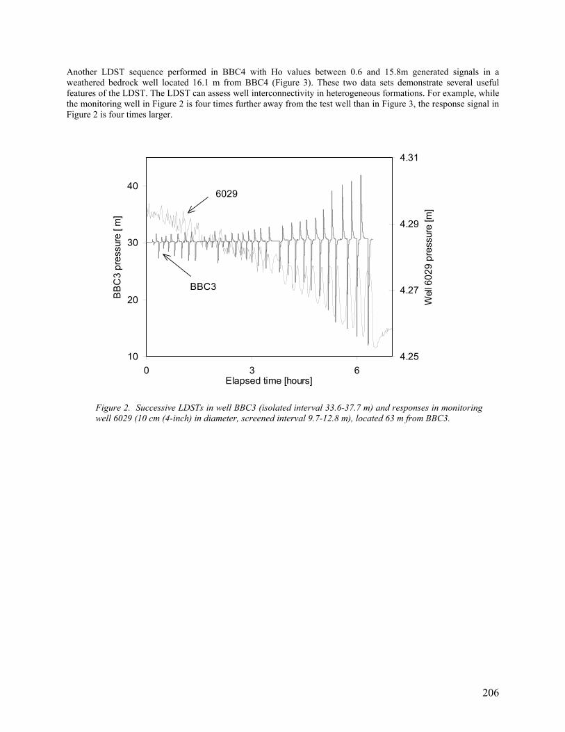
The discrete zones selected for hydraulic testing were isolated with a pneumatic straddle packers system (YEP-4.75/6.00 RoctestTM; Plattsburgh, NY; gland length 1 m). The length of the isolation interval for hydraulic testing was 1.0 or 1.67 m. Within the isolation interval was a perforated 5 cm (2-inch) internal diameter (ID) brass pipe coupled to the packers. The coupling at the base of the bottom packer pipe was capped. The top packer pipe was connected to 5 cm ID threaded aluminum pipe that extended to above the top of the well casing (TOC). Three pressure transducers (RoctestTM PWS vibrating wire; range 0-517 kPa (0-75 psi); accuracy 0.5% full scale; maximum frequency 1 reading each 3 seconds) were included in the system; one just above the top packer, a second in the center of the isolated interval, and a third below the bottom packer. All three transducers were located on the outside of the 5 cm pipe. The upper and lower transducers were used to check the seal between the inflated packers and the wall of the test well; the central transducer records pressure in the isolated zone during hydraulic tests. Packers were inflated with Nitrogen gas (N2). An inflation pressure ~620 kPa (90-psi) in excess of the hydrostatic pressure in each tested interval was sufficient to maintain high integrity packer seals; the deepest BBC well was 62 m, therefore the minimum pressure in the N2 tank regulator was 62 m * 9.8 kPa/m + 620 kPa = 1228 kPa. For simplicity, the inflation pressure in the N2 regulator gauge was set to 1379 kPa (200 psi) for all tested intervals. This pressure met or exceeded the 620 kPa (90 psi) above ambient hydraulic pressure required yet did not exceed manufacturers specifications for maximum packer pressurization. The aluminum pipe at the top of casing was capped with a “T” fitting. A high sensitivity pressure transducer (PDCR 1830 DruckTM; New Fairfield, CT; range 0-345 kPa (0-50 psi); accuracy 0.04% full scale; frequency 64 readings/s) was installed inside the aluminum pipe to a depth below the static water level, expected during the programmed Ho values. This transducer recorded the slug test signals for quantitative analyses. For rising slug tests, the aluminum pipe was pressurized with nitrogen (N2) gas; for falling slug tests the aluminum pipe was depressurized with a vacuum pump. The 2.5 cm (1 inch) wellhead fitting accommodated the slug test transducer cable, the gas line, and a 2.5 cm quick-release ball valve for the pressure release to initiate the ST. Rising slug tests were performed by setting the straddle packer to the desired test depth and inflating the packers. The N2 line was connected to the packer inflation filling at the wellhead. The slug test (Druck) transducer frequency was set to 8 readings/s, and upper, central, and lower transducers (RocTest) to 1 reading/ every 5 seconds. The quick-release valve was left open until all the pressure transducer readings stabilized. The valve was then closed and the N2 tank regulator was set to the programmed pressure for displacing the desired Ho in the test interval. After this pressurization, when all transducer pressure signals had stabilized, the quick-release valve was opened thereby starting the slug test. After one minute, the slug test transducer frequency was decreased to 1 reading every 5 seconds, and after five minutes all transducer frequencies were set to 1 reading per minute. A slug test was considered complete when the water level stabilized in the aluminum pipe, or after 30 minutes duration when testing tight intervals. In the same well intervals, pumping tests were conducted for comparison purposes with the hydraulic parameter estimates of the LDSTs. An electric submersible pump was lowered inside the 5 cm diameter aluminum pipe, down to just above the isolated interval or to a depth greater than the expected drawdown for the pumping test. The central transducer signal was set to a frequency of 1 reading every 5 seconds. Given the low pumping rates (less than 100 ml/s), the flowrate was measured volumetrically each 15 minutes or more frequently when flowrate changes were observed. Recovery data was also collected for pumping tests. All monitoring wells were instrumented with 0-103 kPa (0 – 15 psi) Druck pressure transducers, and set for one 1 reading per minute during hydraulic testing. All pressure transducers were wired to CR10X Campbell ScientificTM dataloggers (Logan, UT). LDST Conceptual Interpretation The complete set of tests for hydraulic characterization of the site, including rising and falling slug tests and short and long pumping tests, was analyzed and reported by Pulido (2003). Several representative LDSTs are presented in this paper to demonstrate the capabilities of the method for hydraulic characterization. A 30 LDST sequence was conducted over the course of 6 hours in an isolated interval in BBC3. Ho values were gradually increased from 60 cm up to 18.9 m. LDST with Ho > 5 m generated water level responses clearly distinguishable from environmental water level fluctuations in the weathered bedrock well 6029 located 63m from the test well (Figure 2).
206
Another LDST sequence performed in BBC4 with Ho values between 0.6 and 15.8m generated signals in a weathered bedrock well located 16.1 m from BBC4 (Figure 3). These two data sets demonstrate several useful features of the LDST. The LDST can assess well interconnectivity in heterogeneous formations. For example, while the monitoring well in Figure 2 is four times further away from the test well than in Figure 3, the response signal in Figure 2 is four times larger.
10
20
30
40
0 3 6Elapsed time [hours]
BB
C3
pres
sure
[ m
]
4.25
4.27
4.29
4.31
Wel
l 602
9 pr
essu
re [m
]
6029
BBC3
Figure 2. Successive LDSTs in well BBC3 (isolated interval 33.6-37.7 m) and responses in monitoring well 6029 (10 cm (4-inch) in diameter, screened interval 9.7-12.8 m), located 63 m from BBC3.
207
30
35
40
45
50
55
0 1 2 3 4 5 6Time [hours]
BB
C4
pres
sure
[m]
0.50
0.51
0.52
0.53
W61
27 p
ress
ure
[m]
BBC4
W6127
Figure 3. Various LDST in well BBC4 (isolated interval 46.1-47.7 m) and responses in monitoring well
6127 (10 cm diameter, screened interval 20.5 – 23.6 m), located 16m from BBC4.
These test also confirm the Ho-duration issue discussed by Chirlin (1990): at each individual LDST, the initial (negative) drawdown during pressurization was persistently lower than the initial (positive) drawdown during release (Figures 2 and 3). This is because pressurization was transmitted to the isolated interval in a gradual way, and a significant formation response occurs during this process. Consequently, the pressurization pulse does not conform to the conceptual model of an instantaneous slug and is not useful for quantitative analysis. On the contrary, the 2.5 cm quick-release valve opening results is a near-instantaneous pressure release. In principle, the monitoring well responses to LDSTs can be used for quantitative estimation of hydraulic parameters. However, the maximum monitoring well response was 2 and 6 mm, respectively (Figures 2 and 3; the transducer accuracy is +/- 1.5 mm). These small variations are enough to demonstrate hydraulic connectivity, but compromise the accuracy of any model that uses this monitoring well data to estimate hydraulic parameters. In addition, the monitoring well storage of water will affect test results (Novakowski, 1989). Therefore, it is desirable to isolate discrete zones in a monitoring well during an LDST in order to increase monitoring well signal size allowing for quantitative analysis.
10
20
30
40
50
10 11 12 13 14 15 16
Time [hours]
BBC
5 pr
essu
re [m
]
39.00
39.25
39.50
39.75
40.00
BBC
4 pr
essu
re [m
]
BBC5
BBC4
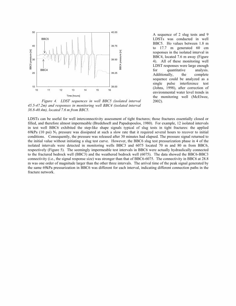
Figure 4. LDST sequences in well BBC5 (isolated interval
45.5-47.2m) and responses in monitoring well BBC4 (isolated interval 38.8-40.4m), located 7.6 m from BBC5.
A sequence of 2 slug tests and 9 LDSTs was conducted in well BBC5. Ho values between 1.8 m to 17.7 m generated 60 cm responses in the isolated interval in BBC4, located 7.6 m away (Figure 4). All of these monitoring well LDST responses were large enough for quantitative analysis. Additionally, the complete sequence could be analyzed as a single pulse interference test (Johns, 1998), after correction of environmental water level trends in the monitoring well (McElwee, 2002).
LDSTs can be useful for well interconnectivity assessment of tight fractures; those fractures essentially closed or filled, and therefore almost impermeable (Bredehoeft and Papadopoulos, 1980). For example, 12 isolated intervals in test well BBC6 exhibited the step-like shape signals typical of slug tests in tight fractures: the applied 69kPa (10 psi) N2 pressure was dissipated at such a slow rate that it required several hours to recover to initial conditions. Consequently, the pressure was released after 30 minutes had elapsed. The pressure signal returned to the initial value without initiating a slug test curve. However, the BBC6 slug test pressurization phase in 4 of the isolated intervals were detected in monitoring wells BBC3 and 6075 located 70 m and 80 m from BBC6, respectively (Figure 5). The seemingly impermeable test intervals in BBC6 were actually hydraulically connected to the fractured bedrock well (BBC3) and the weathered bedrock well (6075). The data showed the BBC6-BBC3 connectivity (i.e., the signal response size) was stronger than that of BBC6-6075. The connectivity in BBC6 at 28.8 m was one order of magnitude larger than the other three intervals. The arrival time of the peak signal generated by the same 69kPa pressurization in BBC6 was different for each interval, indicating different connection paths in the fracture network.
209
0.0
0.1
0.2
0.3
0 6 12 18
Elapsed time after BBC6 pressurization [min]
Wat
er D
epth
Var
iatio
ns fo
r BB
C6
STs
at 2
8.8
m d
epth
[m]
0.00
0.01
0.02
0.03W
ater
dep
th va
riatio
ns fo
r BBC
6 ST
s at
38.
2, 4
7.0,
and
53.
3 m
dep
th [m
]
BBC6 TestedInterval:
47.8 m
53.3 m
28.8 m
38.2 m
BBC3 (solid lines)
W6075 (dashed lines)
Figure 5. Monitoring well BBC3 and 6075 responses to LDST conducted in tight intervals of BBC6.
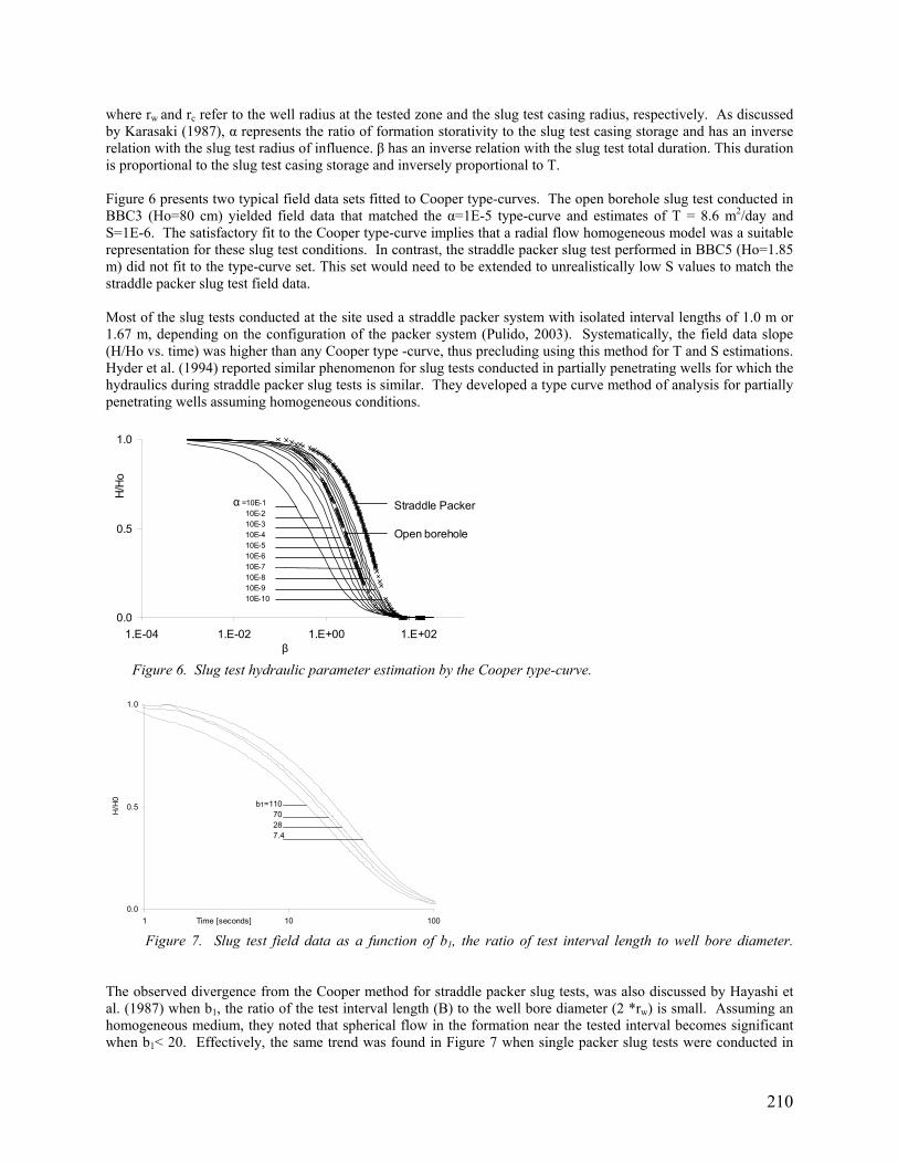
LDST Quantitative Analysis As a first approximation, slug test and LDST field data were fitted to the radial homogeneous model proposed by Cooper et al. (1967). This allowed estimation of T and S values from open borehole slug tests by superimposing the field data onto type-curves depending on the α and β dimensionless parameters defined as:
2
2
c
w
r
Sr=α (1)
2cr
tT=β (2)
210
where rw and rc refer to the well radius at the tested zone and the slug test casing radius, respectively. As discussed by Karasaki (1987), α represents the ratio of formation storativity to the slug test casing storage and has an inverse relation with the slug test radius of influence. β has an inverse relation with the slug test total duration. This duration is proportional to the slug test casing storage and inversely proportional to T. Figure 6 presents two typical field data sets fitted to Cooper type-curves. The open borehole slug test conducted in BBC3 (Ho=80 cm) yielded field data that matched the α=1E-5 type-curve and estimates of T = 8.6 m2/day and S=1E-6. The satisfactory fit to the Cooper type-curve implies that a radial flow homogeneous model was a suitable representation for these slug test conditions. In contrast, the straddle packer slug test performed in BBC5 (Ho=1.85 m) did not fit to the type-curve set. This set would need to be extended to unrealistically low S values to match the straddle packer slug test field data. Most of the slug tests conducted at the site used a straddle packer system with isolated interval lengths of 1.0 m or 1.67 m, depending on the configuration of the packer system (Pulido, 2003). Systematically, the field data slope (H/Ho vs. time) was higher than any Cooper type -curve, thus precluding using this method for T and S estimations. Hyder et al. (1994) reported similar phenomenon for slug tests conducted in partially penetrating wells for which the hydraulics during straddle packer slug tests is similar. They developed a type curve method of analysis for partially penetrating wells assuming homogeneous conditions.
Figure 6. Slug test hydraulic parameter estimation by the Cooper type-curve.
0.0
0.5
1.0
1 10 100Time [seconds]
H/H
0 b1=110 70 28 7.4
Figure 7. Slug test field data as a function of b1, the ratio of test interval length to well bore diameter.
The observed divergence from the Cooper method for straddle packer slug tests, was also discussed by Hayashi et al. (1987) when b1, the ratio of the test interval length (B) to the well bore diameter (2 *rw) is small. Assuming an homogeneous medium, they noted that spherical flow in the formation near the tested interval becomes significant when b1< 20. Effectively, the same trend was found in Figure 7 when single packer slug tests were conducted in
211
BBC3 to isolate progressively smaller intervals from the packer to the bottom of the well (B= 16.7 m (open borehole), 10.7 m, 4.3 m, and 1.12 m; with Ho values of 0.80 m, 1.20 m, 1.24 m, and 1.26m, respectively). When the slug test Ho was progressively increased for a given test interval, the normalized H/Ho field data for each test were not coincident, in contrast to what would be expected from the homogeneous linearity assumption of the Cooper method. Instead, the data plots were shifted towards larger times as Ho was increased. Figure 8 shows this trend for 13 slug tests conducted in BBC5. The observed shift was probably not caused by the larger time required to release the N2 from the slug test casing for larger Ho values because that took less than one second for all Ho.
0.0
1.0
0.1 1 10 100 1000
Time [seconds]
H/H
0
A )Ho=1.85m
B) 3.38
C) 3.62D) 4.78
E) 6.17F) 6.47H) 7.60
I) 9.79J) 11.60K) 13.67L) 14.14M) 15.26
N) 17.70
ABCDE
EDHBAKCMFIJLN
Ho increasing
A) Ho=1.85 m
Figure 8. Normalized slug test data in well BBC5 (isolated interval 45.5-47.2 m) and its dependence on Ho.
McElvee and Zeneer (1998) and McElvee (2002) reported field data dependency on Ho associated with turbulent flow next to and within the test well. Their normalized field curves increased slope as Ho increased. Although the BBC5 data exhibited a temporal offset, the normalized field curves clearly maintained a constant slope with increasing Ho (Figure 8). If turbulent flow existed at the early times because of the large Ho values, the field curve would have exhibited a clear change of shape at the time when the transition to laminar flow was established at the later times. There was no evidence of deviation from laminar (Darcian) flow in the BBC5 curves (Figure 8). Karasaki et al. (1987) analyzed the expected slug test curves when the test well intersects a subhorizontal fracture that is part of an interconnected fracture system. They reasoned that the flow in the intersected fracture is radial and at some distance, where the fracture becomes more interconnected with the fracture system, the flow becomes spherical (as expected when testing a discrete interval in an homogeneous formation). They developed type curves that clearly show the effects of the change in flow geometry from the inner to the outer region. When the total storativity next to the test well is very small, the type curves are shifted horizontally without any noticeable transition from the inner to the outer region. The shift to larger times increases with the ratio between the inner and outer permeabilities. The type curves presented by Hyder et al. (1994), Hayashi et al. (1987) and Karasaki et al. (1987), are not meant to be complete sets of curves for slug test analyses. The application of these methodologies requires developing specific type-curves for the particular hydrogeological conditions expected at the site. Even with customized type-curves, it is likely that field data will not fit a particular type-curve. Either an analytical technique that does not rely on curve matching or a flexible numerical technique are more advantageous for the kind of slug test field data considered in the fractured bedrock wells at the BBC site.
212
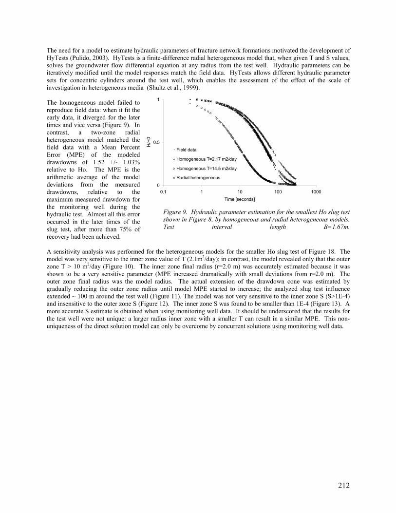
The need for a model to estimate hydraulic parameters of fracture network formations motivated the development of HyTests (Pulido, 2003). HyTests is a finite-difference radial heterogeneous model that, when given T and S values, solves the groundwater flow differential equation at any radius from the test well. Hydraulic parameters can be iteratively modified until the model responses match the field data. HyTests allows different hydraulic parameter sets for concentric cylinders around the test well, which enables the assessment of the effect of the scale of investigation in heterogeneous media (Shultz et al., 1999). The homogeneous model failed to reproduce field data: when it fit the early data, it diverged for the later times and vice versa (Figure 9). In contrast, a two-zone radial heterogeneous model matched the field data with a Mean Percent Error (MPE) of the modeled drawdowns of 1.52 +/- 1.03% relative to Ho. The MPE is the arithmetic average of the model deviations from the measured drawdowns, relative to the maximum measured drawdown for the monitoring well during the hydraulic test. Almost all this error occurred in the later times of the slug test, after more than 75% of recovery had been achieved.
0
0.5
1
0.1 1 10 100 1000Time [seconds]
H/H
0Field data
Homogeneous T=2.17 m2/day
Homogeneous T=14.5 m2/day
Radial heterogeneous
Figure 9. Hydraulic parameter estimation for the smallest Ho slug test shown in Figure 8, by homogeneous and radial heterogeneous models. Test interval length B=1.67m.
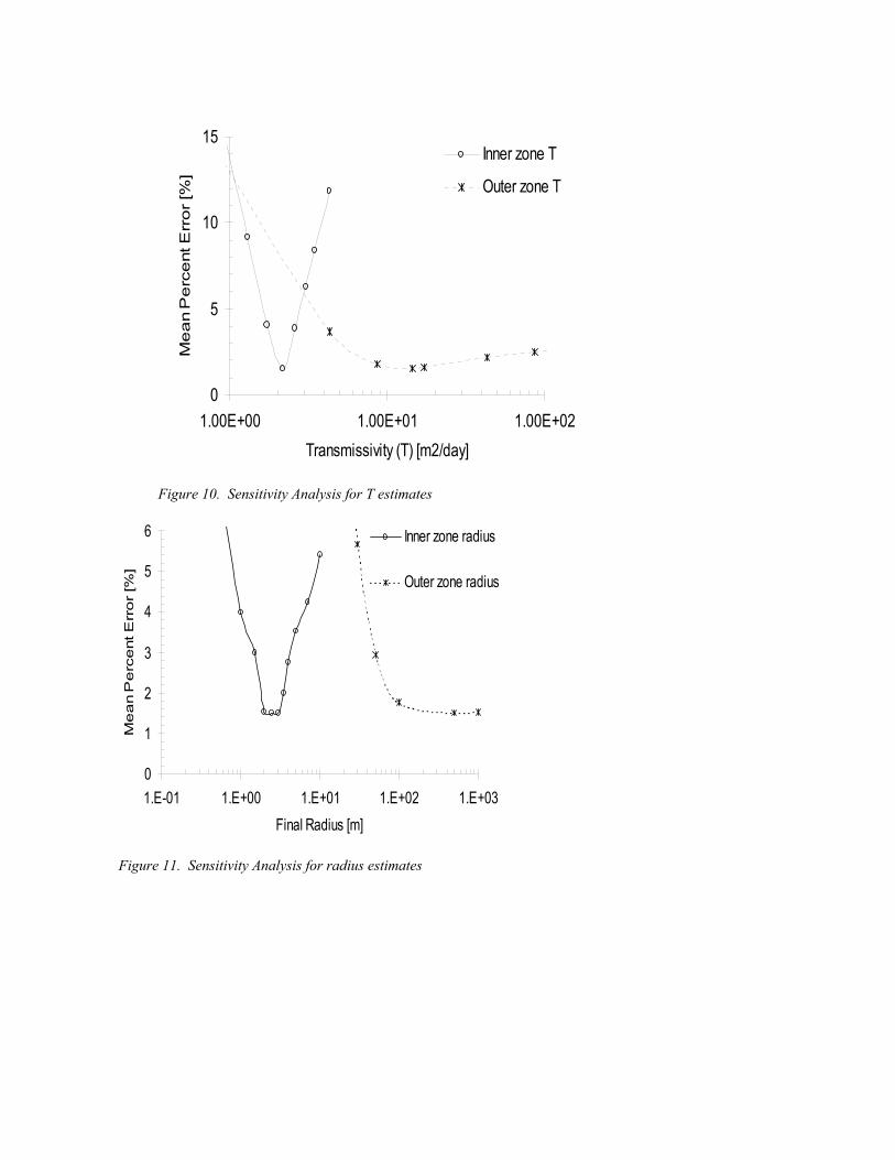
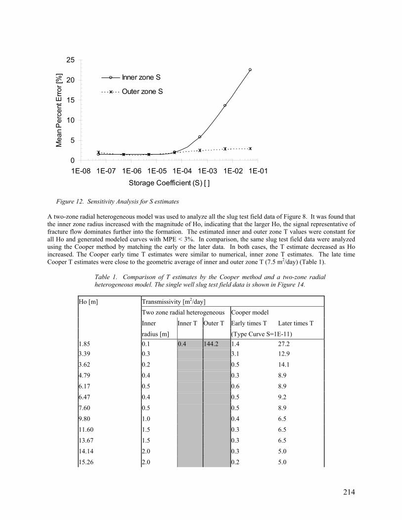
A sensitivity analysis was performed for the heterogeneous models for the smaller Ho slug test of Figure 18. The model was very sensitive to the inner zone value of T (2.1m2/day); in contrast, the model revealed only that the outer zone T > 10 m2/day (Figure 10). The inner zone final radius (r=2.0 m) was accurately estimated because it was shown to be a very sensitive parameter (MPE increased dramatically with small deviations from r=2.0 m). The outer zone final radius was the model radius. The actual extension of the drawdown cone was estimated by gradually reducing the outer zone radius until model MPE started to increase; the analyzed slug test influence extended ~ 100 m around the test well (Figure 11). The model was not very sensitive to the inner zone S (S>1E-4) and insensitive to the outer zone S (Figure 12). The inner zone S was found to be smaller than 1E-4 (Figure 13). A more accurate S estimate is obtained when using monitoring well data. It should be underscored that the results for the test well were not unique: a larger radius inner zone with a smaller T can result in a similar MPE. This non-uniqueness of the direct solution model can only be overcome by concurrent solutions using monitoring well data.
A two-zone radial heterogeneous model was used to analyze all the slug test field data of Figure 8. It was found that the inner zone radius increased with the magnitude of Ho, indicating that the larger Ho, the signal representative of fracture flow dominates further into the formation. The estimated inner and outer zone T values were constant for all Ho and generated modeled curves with MPE < 3%. In comparison, the same slug test field data were analyzed using the Cooper method by matching the early or the later data. In both cases, the T estimate decreased as Ho increased. The Cooper early time T estimates were similar to numerical, inner zone T estimates. The late time Cooper T estimates were close to the geometric average of inner and outer zone T (7.5 m2/day) (Table 1).
Table 1. Comparison of T estimates by the Cooper method and a two-zone radial heterogeneous model. The single well slug test field data is shown in Figure 14.
Ho [m] Transmissivity [m2/day] Two zone radial heterogeneous Cooper model
Pumping test 2.0 0.4 144.2 Values in shade cells are the same for all rows
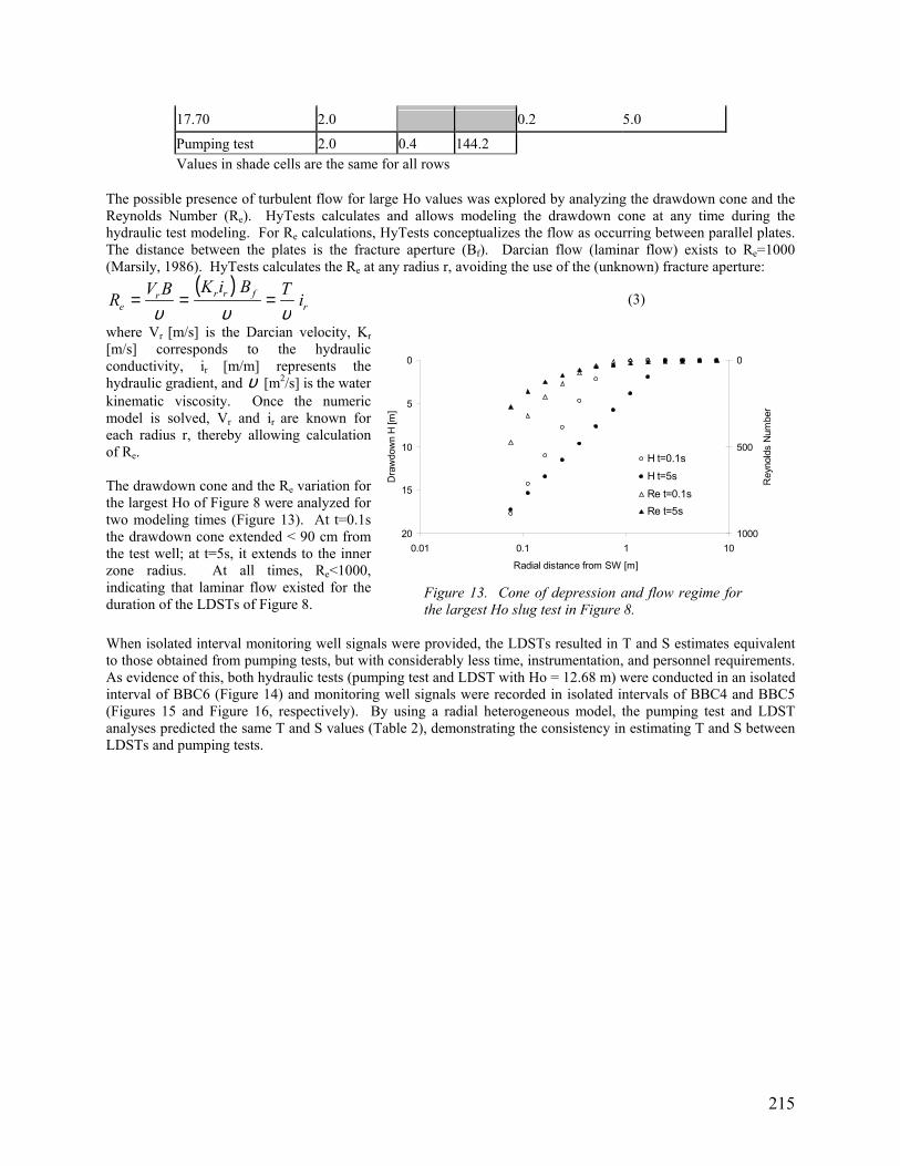
The possible presence of turbulent flow for large Ho values was explored by analyzing the drawdown cone and the Reynolds Number (Re). HyTests calculates and allows modeling the drawdown cone at any time during the hydraulic test modeling. For Re calculations, HyTests conceptualizes the flow as occurring between parallel plates. The distance between the plates is the fracture aperture (Bf). Darcian flow (laminar flow) exists to Re=1000 (Marsily, 1986). HyTests calculates the Re at any radius r, avoiding the use of the (unknown) fracture aperture:
( )r
frrre i
TBiKBVR
υυυ=== (3)
where Vr [m/s] is the Darcian velocity, Kr [m/s] corresponds to the hydraulic conductivity, ir [m/m] represents the hydraulic gradient, and υ [m2/s] is the water kinematic viscosity. Once the numeric model is solved, Vr and ir are known for each radius r, thereby allowing calculation of Re. The drawdown cone and the Re variation for the largest Ho of Figure 8 were analyzed for two modeling times (Figure 13). At t=0.1s the drawdown cone extended < 90 cm from the test well; at t=5s, it extends to the inner zone radius. At all times, Re<1000, indicating that laminar flow existed for the duration of the LDSTs of Figure 8.
0
5
10
15
200.01 0.1 1 10
Radial distance from SW [m]
Dra
wdo
wn
H [m
]
0
500
1000
Rey
nold
s N
umbe
r
H t=0.1s
H t=5s
Re t=0.1sRe t=5s
Figure 13. Cone of depression and flow regime for the largest Ho slug test in Figure 8.
When isolated interval monitoring well signals were provided, the LDSTs resulted in T and S estimates equivalent to those obtained from pumping tests, but with considerably less time, instrumentation, and personnel requirements. As evidence of this, both hydraulic tests (pumping test and LDST with Ho = 12.68 m) were conducted in an isolated interval of BBC6 (Figure 14) and monitoring well signals were recorded in isolated intervals of BBC4 and BBC5 (Figures 15 and Figure 16, respectively). By using a radial heterogeneous model, the pumping test and LDST analyses predicted the same T and S values (Table 2), demonstrating the consistency in estimating T and S between LDSTs and pumping tests.
216
0
5
10
15
20
251.E+00 1.E+02 1.E+04
Time [seconds]
Dra
wdo
wn
[m]
1E-06
1E-05
1E-04
1E-03
1E-02
1E-01
1E+00
PT
Flow
rate
[m3/
s]PT field data
PT Model
ST field data
ST Model
Figure 14. Pumping Test (PT) and LDST conducted in an isolated interval of BBC6.
0.00
0.04
0.08
0.12
0.16
0.201.E+02 1.E+03 1.E+04 1.E+05
Time [seconds]
Dra
wd
ow
n [m
]
PT field data
PT model
ST field data
ST model
Figure 15. Monitoring well BBC4 isolated interval responses to the BBC6 Pumping Test (PT) and LDST shown in Figure 14.
0
0.04
0.08
0.12
0.16
0.21.E+02 1.E+03 1.E+04 1.E+05
Time [seconds]
Dra
wd
ow
n [m
]
PT Field Data
PT Model
ST Field Data
ST Model
Figure 16. Monitoring well BBC5 isolated interval responses to the BBC6 Pumping Test (PT) and LDST shown in Figure 14.
217
Table 2. BBC6 pumping Test (PT) and LDST Comparative Results. (See Figures 14-16 for field data). Test well Monitoring Wells
BBC6 BBC5 BBC4
PT ST PT ST PT ST
Distance from BBC6 [m] 0 7.62 7.62
Depth Top [m] 34.21 36.94 43.56
Bottom [m] 35.89 42.34 45.08
Inner T [m2/day] 0.10 0.10 0.10 0.10 0.10 0.10
Zone S [ ] 7.0E-04 2.0E-04 2.0E-04 2.0E-04
Radius [m] 3.00 3.00 3.00 3.00 3.00 2.00
Central T [m2/day] N/A 1.01 1.01 1.01 0.72
Zone S [ ] 7.0E-04 2.0E-04 2.0E-04 2.0E-04
Radius [m] 10.00 10.00 10.00 10.00
Outer T [m2/day] 14.40 14.40 14.40 14.40 14.40 14.40
Zone S [ ] 7.0E-04 2.0E-04 2.0E-04 2.0E-04
MPE [%] 8.16 3.14 8.47 10.1 6.19 8.25
SD [%] 4.06 2.01 10.9 6.5 4.05 7.71
Shaded cells not applicable (N/A) (two-zone model) The radial heterogeneous model was a first approximation that successfully matched the entire hydraulic test data set from the fractured bedrock formation at the BBC site, meaning that all the modeled curves matched the field data with mean percent errors smaller than 10% (Pulido, 2003). Nevertheless, more sophisticated models are required to capture the fracture network heterogeneity in hydraulic tests analyses. For example, the radial heterogeneous model predicted a gradual start for the BBC5 response to the pumping test conducted in BBC6, however a sudden start for the early time response in BBC5 was observed, indicating more complex hydraulics prevailed (Figure 16). Conclusions LDSTs extend the range of applicability of conventional slug tests, elevating them to the confidence given to pumping test data. By increasing the magnitude of Ho, LDSTs generate water level responses at those monitoring wells that are hydraulically interconnected with the test well. When discrete intervals are isolated in the monitoring well, responses to LDSTs are sufficiently magnified to permit quantitative evaluation of T and S as in pumping tests. However, LDSTs have the advantage of not pumping water and dramatically reducing the required time for testing. LDSTs conducted on tight fractures revealed a detectable hydraulic connection to a well located 70 m from the test well. Slug tests and LDST field normalized data for the BBC wells completed in fractured bedrock, in general did not fit to radial homogeneous models, nor to Cooper type-curves in particular. When Ho increased, the normalized data shifted to increasing times without any change in slope, indicating formation heterogeneity (T) with a constant S. LDSTs can also be used in porous media, as long as the pressurized slug test instrumentation is provided to allow high enough Ho to produce response signals in monitoring wells.
218
A finite difference radial heterogeneous model was successfully used to analyze the slug test and LDST data for this formation, the inner zone T being at least one order of magnitude lower than the outer zone. The inner zone properties were interpreted as representative of single fractures intercepted in the tested well interval and interconnected with the fracture network system at some distance from the test well (outer zone). The estimated inner zone radius increased for larger Ho values. No evidence of turbulent flow was found for the analyzed LDSTs. If turbulent flow exists, a model that includes this hydraulics would need to be adapted to the LDST data. The use of isolated interval monitoring well data together with test well data for LDSTs, allowed reliable estimation of S, and the radius and T values of the outer zone. LDST demonstrated to be consistent with pumping tests in terms of hydraulic parameter estimation. Overall, including LDSTs as part of hydraulic testing activities on hydrogeologic projects will contribute positively to improving the hydrogeological conceptual model of a site. Acknowledgements This research was performed under US EPA contract CR 827878-01-0. The authors would also like to acknowledge the collaboration of the U.S. Air Force and the Pease Development Authority during the BBC project. References
• Belitz K. and Dripps W (1999), Cross-well slug testing in unconfined aquifers: A case study from the Sleepers River Watershed, Vermont. Groundwater 37, no.3: 438 – 447
• Black J.H. and Kipp K.L. (1977), Observation well response time and its effect upon aquifer test results. Journal of Hydrology, 34: 297 – 306
• Bredehoeft J.D. and Papadopoulos S.S. (1980), A Method for determining the hydraulic properties of tight formations, Water Resources Research, Vol.16, No.1, pp 233-238.
• Butler J.J. (1998), The design, performance, and analysis of slug tests, 1st edition, Lewis Publishers, Boca Raton, 252 pp • Chirlin G.R. (1990), The slug test: the first four decades, Groundwater Management 1, no1: 365 - 381 • Cooper H.H., Bredehoeft J.D., and Papadopulos I.S. (1967), Response of a finite-diameter well to an instantaneous charge of water,
Water Resources Research 3, no.1: 263-269. • Hayashi K., Ito T., and Abe H. (1987), A new method for the determination of in situ hydraulic properties by pressure pulse tests and
application to the Higashi Hachimantai Geothermal Field, Journal of Geophysical Research 92, no. B9: 9168-9174 • Hyder Z., Butler J.J., McElwee C.D., and Liu W (1994), Slug tests in partially penetrating wells, Water Resources Research, Vol. 30,
and no.1: 2945-2957. • Hvorslev M.J. (1951), Time lag and soil permeability in ground-water observations, Waterways Experiment Station, Corps of
Engineers, US Army. Bulletin no. 36. • Johns R.T. (1998), Pressure solution for sequential hydraulic tests in low-transmissivity fractured and nonfractured media, Water
Resources Research 34, no.4: 889 - 895 • Karasaki K., Long J.C.S., and Witherspoon P.A. (1988), Analytical models of slug tests, Water Resources Research 24, no.1: 115-126 • Marsily G. (1986), Quantitative Hydrogeology, Academic Press inc., Orlando, 440 pp • McElwee C.D. (2002), Improving the analysis of slug tests, Journal of Hydrology 269: 122-133 • McElwee C.D. and Zenner M.A. (1998), A nonlinear model for analysis of slug-test data, Water Resources Research 34, no.1: 55-66 • Novakowski K.S. (1989), Analysis of pulse interference tests, Water Resources Research, 25, no.11: 2377 – 2387 • Papadopulos I.S., Bredehoeft J.D., and Cooper H.H. (1973), On the analysis of “Slug Test” data, Water Resources Research, 9, no.4:
1087 - 1089 • Pulido G. (2003), Some contributions to the hydraulic characterization of fractured bedrock formations, PhD. Dissertation.
University of New Hampshire. • Shapiro A.M. and Hsieh P.A. (1998), How good are estimates of transmissivity from slug tests in fractures rock?, Groundwater 36,
no.1: 37-48 • Shulze M.D., Carlson D.A., Cherkaurer D.S., and Malik P. (1999), Scale dependency of hydraulic conductivity in heterogeneous
media, Groundwater 27, no. 6:904-919 • Theis C.V. (1935), The relation between the lowering of piezometric surface and the rate and duration of discharge of a well using
ground-water storage, Transactions of American Geophysical Union, 16th annual meeting, pt.2. • Walter G.R. and Thompson G.M. (1982), A repeated pulse technique for determining the hydraulic properties of tight formations,
Groundwater 20, no.2: 186 – 193 • Walton W.C. (1970), Groundwater Resource Evaluation, McGraw-Hill, New York, 664 pp • Wang J.S.Y., Narasimhan T.N., Tsang C.F., and Witherspoon P.A. (1977), Transient flow in tight fractures, Proceedings Invitational
well testing symposium, Lawrence Berkeley Lab., Berkeley: 103-116
219
Biographical Sketches Gonzalo Pulido, PhD is a Hydrogeologist of HydroQual, Inc. He received his PhD in Engineering from University of New Hampshire in 2003. He has over 18 years of academic and consulting experience in groundwater including well drilling, design, installation and hydraulic testing. He has a wide experience in mathematical modeling, including object-oriented programming, computer graphics, and groundwater software development. Thomas P. Ballestero, PhD, PE, PH, CGWP is an Associate Professor at the University of New Hampshire. He received his PhD in Hydrology and Water Resources Engineering from Colorado State University in 1981. Since 1983 he has taught courses water resources engineering at the University of New Hampshire. His general research interests involve the field measurement of hydrologic parameters and the subsequent use of the generated data (statistical inference, modeling, etc.) Nancy E. Kinner, PhD is a Professor at the University of New Hampshire, where she is the Director of the Bedrock Bioremediation Center (BBC), which specializes in multidisciplinary research on bioremediation of organically contaminated bedrock aquifers. Her main areas of research interest are bioremediation of contaminated subsurface environments and more generally, environmental microbiology.