Large-eddy simulation of turbulent open-channel flow over three-

dimensional dunes

ZHIHUA XIE*, Research Associate, School of Engineering, Cardiff University, Cardiff,

CF24 3AA, UK.

Email: zxie@cardiff.ac.uk

BINLIANG LIN (IAHR Member), Professor, State Key Laboratory of Hydroscience and

Engineering, Tsinghua University, Beijing, 10084, China; and School of Engineering, Cardiff

University, Cardiff, CF24 3AA, UK.

Email: linbl@tsinghua.edu.cn (author for correspondence)

ROGER A. FALCONER (IAHR Member), Professor, School of Engineering, Cardiff

University, Cardiff, CF24 3AA, UK.

Email: falconerra@cardiff.ac.uk

TIMOTHY B. MADDUX, Faculty Research Associate, School of Civil and Construction

Engineering, Oregon State University, Corvallis, OR 97331-3212.

Email : tbmaddux@engr.orst.edu

* Present address: Department of Chemical Engineering & Department of Earth Science and

Engineering, Imperial College London, London, SW7 2AZ, UK.

Large-eddy simulation of turbulent open-channel flow over three-

dimensional dunes

ABSTRACT

A large-eddy simulation study has been undertaken to investigate the turbulent structure of open-

channel flow over three-dimensional (3D) dunes. The governing equations have been discretised using

the finite volume method, with the partial cell treatment being implemented in a Cartesian grid form to

deal with the 3D dune topography. The numerical model predicted free surface elevations, mean flow

velocities and Reynolds shear stress distributions have been compared with experimental

measurements published in the literature, with relatively close agreement being obtained between the

two sets of results. The predicted mean velocity field and the associated turbulence structure are

significantly different from those observed for flows over two-dimensional dunes. Due to the dune

three-dimensionality, the model predictions show spanwise variations of mean flow fields, secondary

currents and different distributions of vertical profiles of the double-averaged velocity. Furthermore,

large-scale vortical structures, such as spanwise rollers and hairpin-like structures, are predicted in the

simulations, with most of them being generated in the concave regions of the 3D dunes.

Keywords: Large-eddy simulation, open-channel flow, turbulence, 3D dunes, Cartesian grid

method

1. Introduction

Dunes are ubiquitous bed forms in alluvial channels and play an important role in flow

resistance and sediment transport in many practical hydraulic engineering problems. Over the

past two decades several experimental and numerical model studies have been undertaken for

open-channel flow over dunes, with significant advances having been made in the

understanding of the general features of mean flow and turbulence characteristics. A

comprehensive review of turbulent flow over dunes can be found in Best (2005).

Most of existing experimental studies of turbulent flow over dunes have tended to

focus on the study of two-dimensional (2D) dunes (Müller and Gyr, 1986; van Mierlo and de

Ruiter, 1988; Lyn, 1993; Mclean et al., 1994; Bennett and Best, 1995; Kadota and Nezu,

1999; Hyun et al., 2003, among others). In summarizing these studies it is generally found

that the flow separates at the dune crest and re-attaches at approximately 4-6 dune heights

downstream of the dune crest. A shear layer is generated at the crest, which divides from the

main flow, creating a recirculation zone downstream. A new boundary layer is formed

downstream of the re-attachment point, as the flow re-accelerates and reaches its maximum

velocity at the next dune crest (Best, 2005). Large-scale vortical structures are generated

downstream of the dune crest and tilted upwards, interacting with the free surface to form a

boil (Nezu and Nakagawa, 1993). However, dune three-dimensionality and its implications

remain relatively poorly understood.

Maddux et al. (2003a, b) presented the first detailed experimental study of turbulent

flow over three-dimensional (3D) dunes, in which the height of a dune crest line varied in the

spanwise direction, introducing a 3D topography with a maxima and minima in the crest line

height and with nodes in between. Detailed mean and turbulence characteristics were shown

and compared with 2D dunes. It was found that, although the friction coefficients for flow

over 3D dunes were higher, the turbulence generated by 3D dunes was weaker than their 2D

counterparts due to the generation of secondary circulation. More recently, Venditti (2007)

performed laboratory studies of flow over 3D dunes, in which the dune height and the shape

in the 2D cross-section were fixed, but with a varying dune crest line curvature. The results

suggested that dune three-dimensionality significantly changed the flow field when compared

with 2D dunes and provided a different level of flow resistance. The turbulent kinetic energy

was higher for 3D dunes with lobe-shaped dune crest lines and lower for 3D dunes with

saddle-shaped dune crest lines, when compared to the energy observed over 2D dunes.

Parsons et al. (2005) presented a field study of flow over 3D dunes and found that dune three-

dimensionality was connected to the morphology of the upstream dune. They also found that

3D dunes with lobe and saddle shaped dune crest lines produced smaller separation zones

with higher vertical velocities than 2D straight-crested dunes.

Several numerical model studies of turbulent flow over dunes have been reported in

the literature, which provide more detailed space-time resolutions of the flow field when

compared to experimental investigations, acting as a complementary approach to gain further

insight into the turbulent flow dynamics. Most of the numerical model simulations were based

on the Reynolds-averaged Navier-Stokes (RANS) equations (for example, Mendoza and

Shen, 1990; Johns et al., 1993; Yoon and Patel, 1996), in which all of the unsteadiness is

averaged out and considered as a part of the turbulence, which has been modelled using

various approximate methods. The RANS models are able to provide satisfactory mean flow

fields, but cannot provide detailed instantaneous flow dynamics and coherent turbulent

structures. To overcome these limitations some highly-resolved computations, based on the

LES approach, have recently been performed to simulate turbulent flows over 2D dunes (Yue

et al., 2005a, b, 2006; Stoesser et al., 2008; Grigoriadis et al., 2009; Omidyeganeh and

Piomelli, 2011), in which the mean velocity field, turbulence intensity and Reynolds shear

stresses were predicted. The predictions were found to be generally in good agreement with

corresponding experimental results. Furthermore, the instantaneous velocity fields and large-

scale coherent structures associated with 2D bed forms were presented in detail. Zedler and

Street (2001) presented a detailed LES study of sediment transport in flows over 3D ripples,

which had similar flow features to those over dunes. However, studies reported in the

literature based on LES simulations over 3D dunes still remain limited.

The present paper reports on the use of the LES approach to investigate the turbulent

structure for open-channel flows over 3D dunes, with this being one of the key topics

requiring urgent research to advance our understanding of fluid dynamics over dunes

according to Best (2005). The 3D dune topography deployed in the experimental study by

Maddux et al. (2003a) was used in the present study, as these dunes were qualitatively similar

to real sinuous-crested 3D dunes as observed in the field and in flumes with mobile sediments

(Gabel, 1993). Model predicted free surface elevations, mean velocity field and Reynolds

shear stress distributions are presented and compared with the available detailed experimental

measurements of Maddux et al. (2003a). The present work can be regarded as a

complementary study to existing LES studies, providing an improved understanding of the

flow dynamics over dunes. Details are given in the remainder of the paper of: (i) the

mathematical model and numerical solution method, (ii) the computational model setup, (iii)

the numerical model results and their comparison with the experimental measurements, and

(iv) some conclusions.

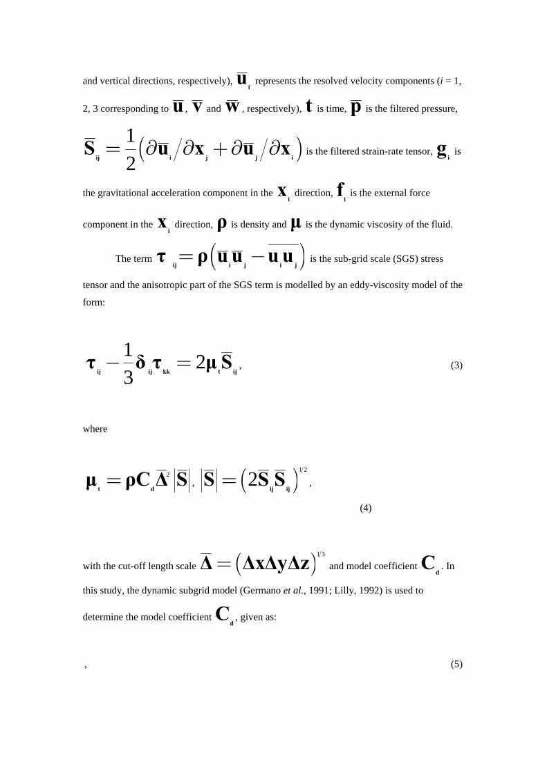
2. Mathematical model and numerical method

The large-eddy simulation approach is adopted in this study, and the governing equations

used are based on the filtered Navier-Stokes equations, given as:

0i

i

u

x

¶=

¶, (1)

2i j ij iji

i i

j i j j

(ρu u ) ( μS ) τ(ρu ) pρg ρf

t x x x x

¶ ¶ ¶¶ ¶+ =- + + + +

¶ ¶ ¶ ¶ ¶, (2)

where the overbar ⋅ denotes the spatial filtering over the grid, i

x represents the Cartesian

coordinates (i = 1, 2, 3 corresponding to x , y and z , meaning the streamwise, spanwise,

and vertical directions, respectively), i

u represents the resolved velocity components (i = 1,

2, 3 corresponding to u , v and w , respectively), t is time, p is the filtered pressure,

( )1

2ij i j j iS u x u x= ¶ ¶ +¶ ¶ is the filtered strain-rate tensor,

ig is

the gravitational acceleration component in the i

x direction, i

f is the external force

component in the i

x direction, ρ is density and μ is the dynamic viscosity of the fluid.

The term ( )ij i j i jτ ρ u u u u= - is the sub-grid scale (SGS) stress

tensor and the anisotropic part of the SGS term is modelled by an eddy-viscosity model of the

form:

12

3ij ij kk t ijτ δ τ μ S- = , (3)

where

2

t dμ ρC Δ S= , ( )

1 2

2ij ij

S S S= ,

(4)

with the cut-off length scale ( )1 3

Δ ΔxΔyΔz= and model coefficient d

C . In

this study, the dynamic subgrid model (Germano et al., 1991; Lilly, 1992) is used to

determine the model coefficient d

C , given as:

, (5)

where Lij uiu j uiu j and

Mij

2 S Sij 2 S Sij

. In these equations, the hat

represents spatial filtering over the test filter. The symbol for spatial filtering is dropped

hereinafter for simplicity.

In this study, the governing equations were discretised using the finite volume

method on a staggered Cartesian grid. The advection terms were discretised by a high-

resolution scheme (Hirsch, 2007), which combined the high order accuracy with

monotonicity, whereas the gradients in pressure and diffusion terms were obtained by central

difference schem12

ij ij

d

ij ij

L MC

M M= es. The SIMPLE algorithm (Patankar, 1980) was

employed for the pressure-velocity coupling and the second-order Gear’s method was used

for the time derivative, which led to an implicit scheme for the governing equations. The code

was parallelised using MPI (Message Passing Interface) and a domain decomposition

technique.

To deal with complex topographies in engineering applications, overlapping grids,

boundary-fitted grids, and unstructured grids can be used. These methods provide great

flexibility to conform onto complex stationary or moving boundaries. However, the

programming of these methods can be complicated and generating such a grid is usually very

cumbersome (Mittal and Iaccarino, 2005). Cartesian grid methods, which can simulate flow

with complex topography on Cartesian grids, avoid these problems. Two of the most popular

methods are the immersed boundary method (Mittal and Iaccarino, 2005) and the Cartesian

cut cell method (Ingram et al., 2003). The primary advantage of a Cartesian grid method is

that only moderate modification of the program on Cartesian grids is needed to account for a

complex topography. A Cartesian grid method also has the advantage of being simple to

generate, particularly with moving boundary problems, due to the use of stationary, non-

deforming grids. However, the drawbacks of this method are that implementing boundary

conditions is not straightforward and the vertical mesh resolution has to be fine enough in the

whole roughness height in order to resolve all turbulent structures in the near-wall region for

complex topography. For LES studies of turbulent flow over 2D dunes, boundary-fitted grids

(Yue et al., 2005a, b, 2006; Stoesser et al., 2008; Omidyeganeh and Piomelli, 2011) and the

immersed bou 0 8xm

L .= ndary method (Grigoriadis et al., 2009) have been previously

used. In the present study, the partial cell treatment developed for 2D by Torrey et al. (1985)

has been extended to 3D and utilized in the finite volume discretisation, in which the

advective and diffusive fluxes at cell faces, as well as the cell volume, have been modified in

cut cells (Xie, 2012).

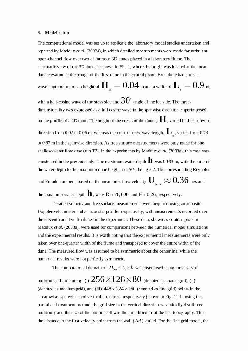
3. Model setup

The computational model was set up to replicate the laboratory model studies undertaken and

reported by Maddux et al. (2003a), in which detailed measurements were made for turbulent

open-channel flow over two of fourteen 3D dunes placed in a laboratory flume. The

schematic view of the 3D dunes is shown in Fig. 1, where the origin was located at the mean

dune elevation at the trough of the first dune in the central plane. Each dune had a mean

wavelength of m, mean height of 0 04m

H .= m and a width of 0 9y

L .= m,

with a half-cosine wave of the stoss side and 30 angle of the lee side. The three-

dimensionality was expressed as a full cosine wave in the spanwise direction, superimposed

on the profile of a 2D dune. The height of the crests of the dunes, H , varied in the spanwise

direction from 0.02 to 0.06 m, whereas the crest-to-crest wavelength, x

L , varied from 0.73

to 0.87 m in the spanwise direction. As free surface measurements were only made for one

shallow-water flow case (run T2), in the experiments by Maddux et al. (2003a), this case was

considered in the present study. The maximum water depth h was 0.193 m, with the ratio of

the water depth to the maximum dune height, i.e. h/H, being 3.2. The corresponding Reynolds

and Froude numbers, based on the mean bulk flow velocity 0 36bulk

U .» m/s and

the maximum water depth h , were 78,000R and 0.26F , respectively.

Detailed velocity and free surface measurements were acquired using an acoustic

Doppler velocimeter and an acoustic profiler respectively, with measurements recorded over

the eleventh and twelfth dunes in the experiment. These data, shown as contour plots in

Maddux et al. (2003a), were used for comparisons between the numerical model simulations

and the experimental results. It is worth noting that the experimental measurements were only

taken over one-quarter width of the flume and transposed to cover the entire width of the

dune. The measured flow was assumed to be symmetric about the centerline, while the

numerical results were not perfectly symmetric.

The computational domain of 2 xm yL L h was discretised using three sets of

uniform grids, including: (i) 256 128 80´ ´ (denoted as coarse grid), (ii)

(denoted as medium grid), and (iii) 448 224 160 (denoted as fine grid) points in the

streamwise, spanwise, and vertical directions, respectively (shown in Fig. 1). In using the

partial cell treatment method, the grid size in the vertical direction was initially distributed

uniformly and the size of the bottom cell was then modified to fit the bed topography. Thus

the distance to the first velocity point from the wall (d ) varied. For the fine grid model, the

grid spacing in terms of wall units was x 80 in the streamwise direction, y 80 in

the spanwise direction, and 0.5 d 8 in the vertical direction. Periodic boundary

conditions were used in the streamwise and spanwise directions. In order to check the

dom352 176 112´ ´ ain size, the distributions of two-point correlation

coefficients of velocities (Moin and Kim, 1982) at two depths (one close to the dune crest and

the other close to the water surface) in the streamwise and spanwise directions are plotted, see

Fig. 2. It can be seen that the two-point correlation coefficients are almost zero at both ends,

which indicates that the computational domain is adequate to contain the largest flow

structures. No-slip boundary conditions were imposed at the dune surface and the free surface

was modelled as a rigid lid (i.e. a free-slip boundary condition), which has been successfully

used in previous LES studies of turbulent open-channel flow (Zedler and Street, 2001; Yue et

al., 2006; Stoesser et al., 2008; Grigoriadis et al., 2009; Omidyeganeh and Piomelli, 2011).

The flow was driven by the external force i

f in the streamwise direction, so that the mean

bulk flow velocity matched the experimental data. The calculations were started with initial

conditions that consisted of the mean bulk flow velocity having random perturbations

superimposed in all three directions. After a statistically steady state was reached, the

simulations were continued for about 10 large-eddy turnover times (i.e. ) for turbulence

statistics.

4. Results and discussion

In the following, the angular bracket, , represents averaging over time, and the resolved

variable is decomposed into a mean value and a resolved fluctuation as:

, (6)

where the prime denotes fluctuation with respect to the mean resolved quantity. A subscript

letter i x , y and z , followed by angular brackets, implies additional spatial averaging of

the mean value over the streamwise ( x), spanwise (

y), and vertical (

z)

directions, respectively. It is worth noting that streamwise and spanwise averaging is

performed at fixed depth levels, with only the flow variables located above the dune surface

being taken into account.

4.1. Spatially averaged mean velocityτ

h / u

An analysis has been undertaken to compare the predicted vertical profiles of the double-

averaged (in the spatial and temporal domains) streamwise velocity (xy

u ) with the

corresponding experimental measurements (Maddux, 2002), see Fig. 3. The graph on the left

hand side of Fig. 3 is a linear plot from the dune trough to the highest crest and the graph on

the right had side is a semi-logarithmic plot of the flow above the mean dune elevation. The

predicted mean velocities were in close agreement with the experimental data, although there

was a discrepancy in the near-bed region, i.e. about 3% relative error for the fine grid.

Differences between the predictions made by the three grids were relatively small, and the

predictions obtained using the fine grid model were closer to the experimental measurements.

Hence only numerical model results obtained for the fine grid model are shown hereinafter.

For open-channel flow over 2D dunes, Mclean et al. (2008) showed that the double-

averaged velocity exhibited a linear profile below the dune crests in the near-bed region and a

logarithmic profile in the outer layer. However, for flow over 3D dunes, an approximately

linear profile in the near-bed region was only observed below the mean dune elevation (i.e.

m/ 0z H ) and the logarithmic profile was only apparent from the mean dune elevation up

to a small elevation above the highest dune crest. The velocity decreased in the vicinity of the

free surface and the characteristic velocity-dip phenomenon for open-channel flows (Nezu

and Nakagawa, 1993) can be observed, which was mainly caused by the secondary currents

(which will be shown later in Fig. 9).

4.2. Free surface elevation

Figure 4 shows a comparison between the measured mean free surface elevation and the

numerical model predicted values, where the predicted free surface elevation was obtained

from the calculated pressure distribution using the rigid lid approximation and then dividing

this value by g. The bed elevation of the 3D dunes is represented by dashed contour lines

along with the plots. The modelled free surface was predicted to increase over the dune

trough and decrease over the dune crest, with slight spanwise variations, which was in good

agreement with the experimental measurements.

Figure 5 shows a comparison between the predicted spanwise-averaged free surface

elevations and experimental measurements, as well as the spanwise-averaged bottom

topography. The predicted free surface correlated well with the dune topography, with there

being a slight phase shift (i.e. approximately 5% of the dune wavelength) between the

modelled and measured mean free surface. The predicted amplitude of the averaged free

surface was approximately 5% lower than the measured value, while a depth-averaged 2D

shallow water model overpredicted the averaged free surface by typically 50% (Maddux et al.,

2003a). It was estimated from Fig. 5 that the difference between the numerical model

predictions for the free surface level obtained using the three grid configurations was less than

2%. Overall, the agreement with the experimental measurements thought to be encouraging,

even though the free surface was treated in the model as a rigid lid.

It is worth noting that the present model correctly predicted the spanwise variation of

the free surface due to the 3D dune topography, whereas a 2D shallow water model predicted

a much stronger spanwise variation than the measured results (Maddux et al., 2003a),

suggesting that non-hydrostatic effects are important in flow over 3D dunes.

4.3. Depth-averaged flow field

Figure 6 shows a comparison between the predicted depth-averaged streamwise and spanwise

velocities and the corresponding experimental measurements. High-speed flow occurred at

the stoss side of the dunes, with the maximum velocity occurring near the node of the dune

crest line (i.e. at 0 225y .= m). In contrast, low-speed flow occurred at the lee

side of the dune, with the minimum velocity occurring downstream of the highest and lowest

parts of the dune crest. It is worth noting that the computed maximum streamwise velocities

occurred at the node of the dune crest line, near the dune crest, which were consistent with the

measurements, and both of which were different from the flow over 2D dunes where the

maxima occurred at the highest dune crest (Maddux et al., 2003a). This was caused by the

dune three-dimensionality, which changed significantly the associated velocity and turbulence

fields.

The spanwise velocities correlated with the 3D dune bathymetry and it can be seen

that the flow was diverted around the 3D dunes. A similar trend of spanwise variation was

observed, where the maxima and minima of the spanwise velocities were located at the node

of the dune crest line near the dune trough, rather than the dune crest in contrast to the

streamwise velocities. Overall, the numerical model predicted the depth-averaged flow fields

to be in good agreement with the experimental measurements of Maddux et al. (2003a).

4.4. Spanwise-averaged flow field

Spanwise-averaged flow fields, including the mean streamwise velocities and Reynolds shear

stress, are presented in this section. In addition, in order to show the flow response to the

effects of three-dimensionality of the dune bathymetry, the mean streamwise velocities and

Reynolds shear stresses at two spanwise locations (i.e. the centerline 0y = m, and the

node along the crest line 0 225y .=- m, which is half way between the highest

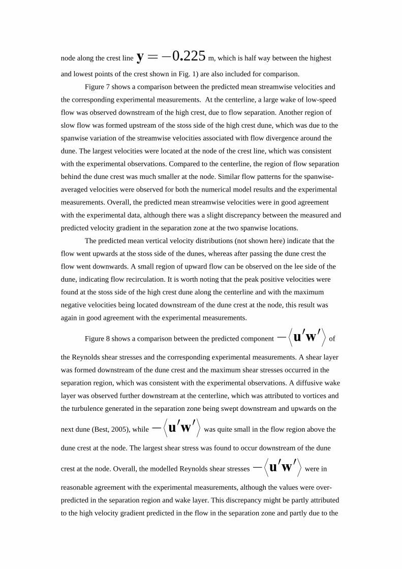
and lowest points of the crest shown in Fig. 1) are also included for comparison.

Figure 7 shows a comparison between the predicted mean streamwise velocities and

the corresponding experimental measurements. At the centerline, a large wake of low-speed

flow was observed downstream of the high crest, due to flow separation. Another region of

slow flow was formed upstream of the stoss side of the high crest dune, which was due to the

spanwise variation of the streamwise velocities associated with flow divergence around the

dune. The largest velocities were located at the node of the crest line, which was consistent

with the experimental observations. Compared to the centerline, the region of flow separation

behind the dune crest was much smaller at the node. Similar flow patterns for the spanwise-

averaged velocities were observed for both the numerical model results and the experimental

measurements. Overall, the predicted mean streamwise velocities were in good agreement

with the experimental data, although there was a slight discrepancy between the measured and

predicted velocity gradient in the separation zone at the two spanwise locations.

The predicted mean vertical velocity distributions (not shown here) indicate that the

flow went upwards at the stoss side of the dunes, whereas after passing the dune crest the

flow went downwards. A small region of upward flow can be observed on the lee side of the

dune, indicating flow recirculation. It is worth noting that the peak positive velocities were

found at the stoss side of the high crest dune along the centerline and with the maximum

negative velocities being located downstream of the dune crest at the node, this result was

again in good agreement with the experimental measurements.

Figure 8 shows a comparison between the predicted component u w¢ ¢- of

the Reynolds shear stresses and the corresponding experimental measurements. A shear layer

was formed downstream of the dune crest and the maximum shear stresses occurred in the

separation region, which was consistent with the experimental observations. A diffusive wake

layer was observed further downstream at the centerline, which was attributed to vortices and

the turbulence generated in the separation zone being swept downstream and upwards on the

next dune (Best, 2005), while u w¢ ¢- was quite small in the flow region above the

dune crest at the node. The largest shear stress was found to occur downstream of the dune

crest at the node. Overall, the modelled Reynolds shear stresses u w¢ ¢- were in

reasonable agreement with the experimental measurements, although the values were over-

predicted in the separation region and wake layer. This discrepancy might be partly attributed

to the high velocity gradient predicted in the flow in the separation zone and partly due to the

fact that the periodic boundary conditions used in the simulation were different from the

actual flow condition in the experiment, which was not exactly periodic in the streamwise

direction (Maddux et al., 2003b) and which could have enhanced the turbulence levels in the

simulations, with this phenomena having been observed in a previous study of flow over 2D

dunes by Dimas et al. (2008).

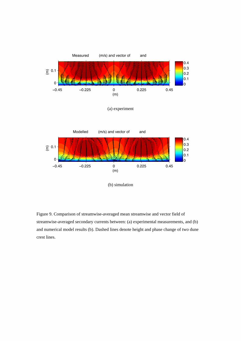
4.5. Streamwise-averaged flow field

Figure 9 shows a comparison between the predicted streamwise-averaged mean streamwise

velocities and secondary currents and the corresponding experimental measurements, along

with dashed lines denoting the height and phase change of the two dune crest lines. The

streamwise velocities were observed to be largest at the node of the crest line, as discussed in

the depth-averaged and spanwise-averaged flow fields. It can be seen from the streamwise

(x

u ) velocity and vectors of (x

v ,x

w ) that the high-speed fluid occurred at the

node of the crest line moving downwards, whereas the low-speed fluid occurred at the

centerline, moving upwards. The secondary currents showed a system of four counter-rotating

circulation areas, which was consistent with the experimental observations. The predicted

values of the secondary flow near the bed were higher than the experimental measurements,

which might be partly due to the enhanced spanwise variation by the periodic boundary

condition and partly due to first-order errors introduced in the partial cell treatment, using the

cut-cell method. However as the secondary current velocities were just over 5% of the mean

bulk flow velocity (Maddux et al., 2003a), this effect of this discrepancy was relatively small.

Overall, satisfactory agreement was obtained between the predicted streamwise-averaged

mean velocities and the corresponding experimental measurements.

In order to demonstrate the three-dimensional characteristics of the flow field, the

mean streamwise velocities and secondary currents at the two maximum dune crests in the

streamwise direction are shown in Fig. 10. It can be seen that the mean flow field varies in the

cross section as well as in the streamwise direction due to the three-dimensionality of the

dune, which is different from the flow over 2D dunes where the cross-variation of the flow

field is normally not observed. At these two cross sections, similar distribution of the

streamwise velocity along the node was observed, whereas the streamwise velocity changed

significantly along the centerline due to the bed topography. The spanwise velocities show

that the fluid diverted around the 3D dunes in the lower flow region, while the upper flow

region moved in the opposite direction. The vertical velocities show that the flow moved

towards the free surface near the dune crest and trough, while upward and downward flows

were observed near the node. Strong secondary currents were observed near the wall region at

the cross section where the dune is highest at the center. These results suggest the flow

pattern over a 3D dune is different from that over a 2D dune, which may have an implication

on the turbulent structures.

4.6. Instantaneous flow and coherent structures

Figure 11 shows the instantaneous flow structures at one instant in time, where Fig. 11(a)

depicts the locations of the three planes selected to show the details of the instantaneous

streamwise velocity u and the perturbation velocity vectors ( , ,u v w ), namely: a central

plane at 0y m (Fig. 11(b)), a horizontal plane just above the highest dune crest at

0.04z m (Fig. 11(c)), and a streamwise plane in the middle of the domain at 0.8x m

(Fig. 11(d)).

At the x z plane (Fig. 11(b)), the instantaneous streamwise velocity distribution

had a similar trend to that of the mean streamwise velocity distribution shown in Fig. 7, with

a recirculation zone again being observed downstream of the dune crest, but with a different

length of re-attachment. The bursting phenomena occurring in the flow could be observed

from the velocity fluctuation vectors, in which the second quadrant Q2 ( 0u , 0w )

corresponded to the ‘ejection’ events, indicating outflow of low-speed fluid, and the fourth

quadrant Q4 (, w 0 ) corresponded to the ‘sweep’ events, indicating inflow of high speed-

fluid (Lu and Willmarth, 1973). Strong ‘ejection’ and ‘sweep’ turbulent events were found in

the near wall region, which were the main contribution to the Reynolds stresses in the

turbulent boundary layer. Across the x y plane (Fig. 11(c)), the flow along the node moved

faster than the flow along the centerline, which was similar to the depth-averaged flow field

shown in Fig. 6. Negative streamwise velocities were found downstream of the highest dune

crest. It can be seen from the velocity fluctuation vectors that a largely chaotic flow was

produced in the separation region and the flow was more turbulent in the lee side of the

highest dune crest than other areas. It can be seen from Fig. 11(d) that the instantaneous

velocities across the y z plane are different from the time-averaged secondary currents

shown in Fig. 9. Near the bed, the low-speed fluid moved away from the wall, suggesting

strong ‘ejection’ events near the separation zone. Figure 11 shows that the turbulent flow

fields over the 3D bed topography vary significantly in the streamwise and spanwise

directions, which are different from the velocity distributions observed for flow over 2D

dunes.

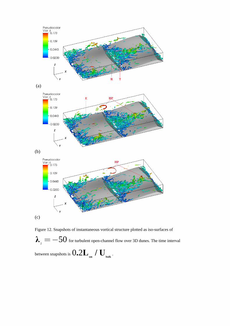
The large-scale coherent structures generated behind the dunes play an essential role

in the interaction between the bed and free surface, sediment transport, and bed form

evolution in open-channel flows. The dynamics of the coherent structures also affects the

mass exchange processes in channel flows (Constantinescu et al., 2009). In order to illustrate

the coherent vortical 0u structure developed over the 3D dunes, the 2

λ method (Jeong

and Hussain, 1995) was used in the present study to identify vortex cores, based on the

second invariant of the velocity gradient tensor. Figure 12 shows three snapshots of

instantaneous vortical structures developed in the flow over 3D dunes, for a constant time

interval of 0 2xm bulk

. L / U . The vortical structures were plotted as iso-surfaces of

2 50 and coloured according to the vertical distance z . Spanwise rollers (labelled R in

Fig. 12(a)) were generated in the separation zone due to Kelvin-Helmholtz instability. They

were advected downstream in a vortex pairing process and interacted with the near wall

structures. As a result of the vortex-wall interaction, three-dimensional tube-like (labelled T

in Fig. 12(a)) vortical structures were produced from the re-attachment point, with complex

temporal and spatial interactions occurring between these vortical structures. As the vortical

structures moved downstream, some of them became elongated (labelled E in Fig. 12(b)) due

to vortex stretching and then broke up into small-scale vortices (Fig. 12(c)) just upstream of

the next dune crest. Some of these vortical structures were also swept downstream and tilted

upwards (observed as hairpin-like structures – labelled HP in Fig. 12(b)), occupying most of

the flow depth and reaching the free surface in some cases (Fig. 12(c)). This phenomenon is

consistent with the observations made by Nezu and Nakagawa (1993) for flows over 2D

dunes. The development of vortical structures was similar to that observed in turbulent

channel flows, where Q2 events occurred between the vortex legs and Q4 events were found

outside the legs (Robinson, 1991).

In contrast to the flow over 2D dunes, there is a significant variation of coherent

structures developed in flow over 3D dunes. It can be observed from the highly three-

dimensional and energetic flow structures that most of the vortices were generated in the

concave region of the 3D dunes, with a spanwise variation of the distribution of coherent

structures. This is attributed to the largest separation region occurred downstream of the

highest dune crest in the spanwise direction, where the rate of strain is high. In addition, the

secondary currents appearing in the flow over 3D dunes (Figs. 9 and 10) also significantly

affect the large-scale coherent structures. In the lower part of the flow, the vortical structures

generated in the shear layer tend to move towards the centerline, enhancing the vortex lift up

process, whereas in the upper part of the flow, the vortical structures tend to move towards

the node, slowing the lift up process.

5. Conclusions

In this paper a large-eddy simulation model of turbulent open-channel flow over three-

dimensional dunes has been presented and compared with available experimental data at

Reynolds numbers of typically 78 000, . The partial cell treatment method on a

Cartesian grid has been used to represent the complex 3D dune topography, which differs

from the boundary-fitted grids and immersed boundary method used in previous 2D dune

studies.

The principal flow features measured in the experiments of Maddux et al. (2003a),

were successfully reproduced, including: the free surface elevations, double-averaged

velocity profile, the depth-averaged mean velocity field, and the spanwise- and streamwise-

averaged mean velocity fields. However, the model over-predicted the Reynolds shear

stresses and this is thought to be due mainly to the periodic boundary conditions used in the

simulations being different from the actual flow conditions in the experiments.

Some of the general features observed in flows over 2D dunes, such as flow

separation at the dune crest and turbulence generation in the shear layer, were also observed

in flows over 3D dunes. The model predicted different double-averaged velocity profiles and

strong spanwise variation of flow fields in flows over 3D dunes. The dune three-

dimensionality altered the mean flow field and the associated turbulence structure observed

over 2D dunes, which could be responsible for the generation of the system of four counter-

rotating secondary currents directing high-speed fluid downwards and low-speed fluid

upwards. Instantaneous velocity fluctuation fields were also shown with the ‘ejection’ and

‘sweep’ turbulent events, which play an essential role in the processes of sediment transport

and bed form evolution in open-channel flows. It was found in this study that the

instantaneous flow was highly three-dimensional with a largely chaotic flow being produced

in the separation region and the flow was more turbulent in the lee side of the highest dune

crest than other areas. It was also found that the large-scale vortical structures, i.e. spanwise

rollers and hairpin-like structures, were generated mostly in the concave regions of the 3D

dunes partly due to the largest separation region downstream of the highest dune crest and

partly due to the secondary currents.

Acknowledgements

The research was supported by the UK Engineering and Physical Sciences Research Council

(EP/G014264/1). This work was performed using the computational facilities of the

Advanced Research Computing @ Cardiff (ARCCA) Division, Cardiff University.

Constructive comments from anonymous reviewers and the associate editor for the

improvement of the manuscript are gratefully acknowledged.

Notation

dC = dynamic subgrid model coefficient

F = Froude number

= external force components

gi = gravitational acceleration components

h = maximum water depth

H = dune height

Hm = dune mean height

Lx = dune wavelength

Lxm = dune mean wavelength

Ly = dune width

Lij = tensor used in dynamic subgrid model

Mij = tensor used in dynamic subgrid model

p = filtered pressure

R = Reynolds number

Sij = filtered strain-rate tensor

t = time

Ubulk = mean bulk flow velocity

u = fluid shear velocity

ui = resolved velocity components

ui

f = resolved streamwise velocity

v = resolved spanwise velocity

w = resolved vertical velocity

u w = shear stress

= Cartesian coordinates

x = streamwise direction

y = spanwise direction

z = vertical direction

= density of the fluid

= dynamic viscosity of the fluid

t = turbulent eddy viscosity

ij = subgrid-scale (SGS) stress tensor

= filter length scale

2 = value used in the 2method

i

x = arbitrary variable

= filtered variable

= spatial filtering variable over the test filter

= variable fluctuation

= mean variable

x = streamwise-averaged mean variable

y = spanwise-averaged mean variable

z = depth-averaged mean variable

References

Bennett, S. J., Best, J.L. (1995). Mean flow and turbulence structure over fixed, 2-

dimensional dunes - implications for sediment transport and bedform stability.

Sedimentology. 42 (3), 491–513.

Best, J. (2005). The fluid dynamics of river dunes: A review and some future research

directions. J. Geophys. Res. 110, F04S02.

Constantinescu, G., Sukhodolov, A., McCoy, A. (2009). Mass exchange in a shallow channel

flow with a series of groynes: LES study and comparison with laboratory and field

experiments. Environ. Fluid Mech. 9 (6), 587–615.

Dimas, A.A., Fourniotis, N.T., Vouros, A.P., Demetracopoulos, A.C. (2008). Effect of bed

dunes on spatial development of open-channel flow. J. Hydraulic Res. 46 (6), 802–813.

Gabel, S.L. (1993). Geometry and kinematics of dunes during steady and unsteady flows in

¢ the Calamus River, Nebraska, USA. Sedimentology, 40(2), 237–269.

Germano, M., Piomelli, U., Moin, P., Cabot, W.H. (1991). A dynamic subgrid-scale eddy

viscosity model. Phys. Fluids A. 3 (7), 1760–1765.

Grigoriadis, D.G.E., Balaras, E., Dimas, A.A. (2009). Large-eddy simulations of

unidirectional water flow over dunes. J. Geophys. Res. 114, F02022.

Hirsch, C. (2007). Numerical computation of internal and external flows introduction to the

fundamentals of CFD. new ed. Butterworth-Heinemann, Oxford.

Hyun, B.S., Balachandar, R., Yu, K., Patel, V.C. (2003). Assessment of PIV to measure mean

velocity and turbulence in open-channel flow. Exp. Fluids. 35 (3), 262–267.

Ingram, D.M., Causon, D.M., Mingham, C.G. (2003). Developments in Cartesian cut cell

methods. Math. Comput. Simulat. 61(3-6), 561–572.

Jeong, J., Hussain, F. (1995). On the identification of a vortex. J. Fluid Mech. 285, 69–94.

Johns, B., Soulsby, R.L., Xing, J.X. (1993). A comparison of numerical-model experiments

of free-surface flow over topography with flume and field observations. J. Hydraulic

Res. 31 (2), 215–228.

Kadota, A., Nezu, I. (1999). Three-dimensional structure of space-time correlation on

coherent vortices generated behind dune crest. J. Hydraulic Res. 37 (1), 59–80.

Lilly, D.K. (1992). A proposed modification of the Germano-subgrid-scale closure method.

Phys. Fluids A. 4 (3), 633–635.

Lu, S.S., Willmarth, W.W. (1973). Measurements of the structure of the Reynolds stress in a

turbulent boundary layer. J. Fluid Mech., 60, 481–511.

Lyn, D.A. (1993). Turbulence measurements in open-channel flows over artificial bed forms.

J. Hydraulic Eng. 119 (3), 306–326.

Maddux, T.B. (2002). Turbulent open channel flow over fixed three-dimensional dune

shapes. Ph.D. thesis, Univ. of Calif., Santa Barbara.

Maddux, T.B., Nelson, J.M., McLean, S.R. (2003a). Turbulent flow over three-dimensional

dunes: 1. free surface and flow response. J. Geophys. Res. 108 (F1), 6009.

Maddux, T.B., McLean, S.R., Nelson, J.M. (2003b). Turbulent flow over three-dimensional

dunes: 2. fluid and bed stresses. J. Geophys. Res. 108 (F1), 6010.

Mclean, S.R., Nelson, J.M., Wolfe, S.R. (1994). Turbulence structure over 2-dimensional bed

forms - implications for sediment transport. J. Geophys. Res. 99 (C6), 12,729–12,747.

Mclean, S.R., Nikora, V.I., Coleman, S.E. (2008) Double-averaged velocity profiles over

fixed dune shapes. Acta Geophysica, 56 (3), 669–697.

Mendoza, C., Shen, H.W. (1990). Investigation of turbulent flow over dunes. J. Hydraulic

Eng. 116 (4), 459–477.

Mittal, R., Iaccarino, G. (2005). Immersed boundary methods. Annu. Rev. Fluid Mech. 37,

239–261.

Müller, A., Gyr, A. (1986). On the vortex formation in the mixing layer behind dunes. J.

Hydraulic Res. 24 (5), 359–375.

Moin, P, Kim, J. (1982). Numerical investigation of turbulent channel flow. J. Fluid Mech.,

118, 341–377.

Nezu, I., Nakagawa, H. (1993). Turbulence in open-channel flows, International Association

for Hydraulic Research monograph series. A.A. Balkema, Rotterdam.

Omidyeganeh, M., Piomelli, U. (2011). Large-eddy simulation of two-dimensional dunes in a

steady, unidirectional flow. J. Turbulence, 12 (42), 1–31.

Parsons, D.R., Best, J.L., Orfeo, O., Hardy, R.J., Kostaschuk, R., Lane, S.N. (2005).

Morphology and flow fields of three-dimensional dunes, Rio Parana, Argentina: Results

from simultaneous multibeam echo sounding and acoustic Doppler current profiling. J.

Geophys. Res. 110, F04S03.

Patankar, S.V. (1980). Numerical heat transfer and fluid flow. Taylor & Francis, London.

Robinson, S.K. (1991). Coherent motions in the turbulent boundary layer. Annu. Rev. Fluid

Mech. 23, 601–639.

Stoesser, T., Braun, C., Garcia-Villalba, M., Rodi, W. (2008). Turbulence structures in flow

over two-dimensional dunes. J. Hydraulic Eng. 134 (1), 42–55.

Torrey, M.D., Cloutman, L.D., Mjolsness, R.C., Hirt, C.W. (1985). NASA-VOF2D: a

computer program for incompressible flows with free surfaces. Tech. Rep. LA-10612-

MS, Los Alamos Scientific Laboratory.

van Mierlo, M.C.L.M, de Ruiter, and J.C.C. (1988). Turbulence measurements above

artificial dunes. Tech. Rep. Q789, Delft Hydraulics Laboratory, Delft, Netherlands.

Venditti, J.G. (2007). Turbulent flow and drag over fixed two- and three-dimensional dunes.

J. Geophys. Res. 112, F04008.

Xie, Z. (2012). Numerical study of breaking waves by a two-phase flow model. Int. J. Numer.

Methods Fluids, 70 (2), 246–268.

Yoon, J.Y., Patel, V.C. (1996). Numerical model of turbulent flow over sand dune. J.

Hydraulic Eng. 122 (1), 10–18.

Yue, W.S., Lin, C.L., Patel, V.C. (2005a). Large eddy simulation of turbulent open-channel

flow with free surface simulated by level set method. Phys. Fluids. 17 (2), 025108.

Yue, W.S., Lin, C.L., Patel, V.C. (2005b). Coherent structures in open-channel flows over a

fixed dune. J. Fluids Eng. 127 (5), 858–864.

Yue, W.S., Lin, C.L., Patel, V.C. (2006). Large-eddy simulation of turbulent flow over a

fixed two-dimensional dune. J. Hydraulic Eng. 132 (7), 643–651.

Zedler, E.A., Street, R.L. (2001). Large-eddy simulation of sediment transport: Currents over

ripples. J. Hydraulic Eng. 127 (6), 444–452.

Figure captions

Figure 1. Schematic of computational domain for turbulent open-channel flow over three-

dimensional dunes with numerical grid (only several grid lines plotted). Centerline

at 0y = m, and node of crest line at 0 225y .= m (half-way between

highest and lowest points of crest) are also shown.

Figure 2. Two-point correlations of the velocity components in the x y planes close to the

dune crest ( 0.4z h ) and close to the water surface ( 0.8z h ): (a) streamwise distribution;

(b) spanwise distribution.

Figure 3. Comparison of spatially-averaged mean velocity profiles between experimental

measurements and numerical model results.

Figure 4. Comparison of mean free surface elevation between: (a) experimental

measurements, and (b) numerical model results. Bed elevation contours are represented by

dashed lines in this and subsequent figures.

Figure 5. Comparison of spanwise-averaged free surface elevation between experimental

measurements and numerical model results (top) and spanwise-averaged bottom topography

(bottom).

Figure 6. Comparison of depth-averaged streamwise (top) and spanwise (bottom) velocities

between: (a) experimental measurements, (b) and numerical model results, and (c) their direct

comparison along the centerline and node.

Figure 7. Comparison of mean streamwise velocities along centerline ( 0y = m, top) and

node ( 0 225y .= - m, middle), and spanwise-averaged streamwise velocities (bottom)

between experimental measurements and numerical model results. Results are shown from

0.1 m to 1.5 m with 0.1 m interval and the arrows denote a magnitude of 0.5 m/s.

Figure 8. Comparison of Reynolds shear stresses at centerline ( 0y = m, top) and node

( 0 225y .= - m, middle), and spanwise-averaged Reynolds shear stresses (bottom) between

experimental measurements and numerical model results. Results are shown from 0.1 m to

1.5 m with 0.1 m interval and the arrows denote a magnitude of 0.003 m2/s2.

Figure 9. Comparison of streamwise-averaged mean streamwise and vector field of

streamwise-averaged secondary currents between: (a) experimental measurements, and (b)

and numerical model results (b). Dashed lines denote height and phase change of two dune

crest lines.

Figure 10. Mean streamwise velocity distribution and vector field of secondary currents along

the two maximum dune crest in the streamwise direction.

Figure 11. Contours of the instantaneous streamwise velocity with perturbation velocity

vectors at (b) x z- , (c) x y- , and (d) y z- planes. The locations of the three

planes are shown in (a).

Figure 12. Snapshots of instantaneous vortical structure plotted as iso-surfaces of

250λ =- for turbulent open-channel flow over 3D dunes. The time interval

between snapshots is 0 2xm bulk

. L / U .

Figure 1. Schematic of computational domain for turbulent open-channel flow over three-

dimensional dunes with numerical grid (only several grid lines plotted). Centerline

at 0y = m, and node of crest line at 0 225y .= m (half-way between

highest and lowest points of crest) are also shown.

(a) (b)

Figure 2. Two-point correlations of the velocity components in the x y planes close to the

dune crest ( 0.4z h ) and close to the water surface ( 0.8z h ): (a) streamwise distribution;

(b) spanwise distribution.

Figure 3. Comparison of spatially-averaged mean velocity profiles between experimental

measurements and numerical model results.

(a) experiment

(b) simulation

Figure 4. Comparison of mean free surface elevation between: (a) experimental

measurements, and (b) numerical model results. Bed elevation contours are represented by

dashed lines in this and subsequent figures.

Figure 5. Comparison of spanwise-averaged free surface elevation between experimental

measurements and numerical model results (top) and spanwise-averaged bottom topography

(bottom).

(a) experiment (b) simulation (c) comparison

Figure 6. Comparison of depth-averaged streamwise (top) and spanwise (bottom) velocities

between: (a) experimental measurements, (b) and numerical model results, and (c) their direct

comparison along the centerline and node.

0 0.4 0.8 1.2 1.6

0

0.1

x (m)

z (m

)

<u> (m/s) over 3d dunes, centerline

EXPLES

0 0.4 0.8 1.2 1.6

0

0.1

x (m)

z (m

)

<u> (m/s) over 3d dunes, node

0 0.4 0.8 1.2 1.6

0

0.1

x (m)

z (m

)

<u>y (m/s) over 3d dunes, spanwise average

Figure 7. Comparison of mean streamwise velocities along centerline ( 0y = m, top) and

node ( 0 225y .= - m, middle), and spanwise-averaged streamwise velocities (bottom)

between experimental measurements and numerical model results. Results are shown from

0.1 m to 1.5 m with 0.1 m interval and the arrows denote a magnitude of 0.5 m/s.

Figure 8. Comparison of Reynolds shear stresses at centerline ( 0y = m, top) and node

( 0 225y .= - m, middle), and spanwise-averaged Reynolds shear stresses (bottom) between

experimental measurements and numerical model results. Results are shown from 0.1 m to

1.5 m with 0.1 m interval and the arrows denote a magnitude of 0.003 m2/s2.

(a) experiment

(b) simulation

Figure 9. Comparison of streamwise-averaged mean streamwise and vector field of

streamwise-averaged secondary currents between: (a) experimental measurements, and (b)

and numerical model results (b). Dashed lines denote height and phase change of two dune

crest lines.

Figure 10. Mean streamwise velocity distribution and vector field of secondary currents along

the two maximum dune crest in the streamwise direction.

(a)

(b)

(c)

(d)

Figure 11. Contours of the instantaneous streamwise velocity with perturbation velocity

vectors at (b) x z- , (c) x y- , and (d) y z- planes. The locations of the three

planes are shown in (a).

(a)

(b)

(c)

Figure 12. Snapshots of instantaneous vortical structure plotted as iso-surfaces of

250λ =- for turbulent open-channel flow over 3D dunes. The time interval

between snapshots is 0 2xm bulk

. L / U .