LARGE FORCE SHAPE MEMORY ALLOY LINEAR ACTUATOR By JOSÉ R. SANTIAGO ANADÓN A THESIS PRESENTED TO THE GRADUATE SCHOOL OF THE UNIVERSITY OF FLORIDA IN PARTIAL FULFILLMENT OF THE REQUIREMENTS FOR THE DEGREE OF MASTER OF SCIENCE UNIVERSITY OF FLORIDA 2002
Transcript
LARGE FORCE SHAPE MEMORY ALLOY LINEAR ACTUATOR
By
JOSÉ R. SANTIAGO ANADÓN
A THESIS PRESENTED TO THE GRADUATE SCHOOL OF THE UNIVERSITY OF FLORIDA IN PARTIAL FULFILLMENT
OF THE REQUIREMENTS FOR THE DEGREE OF MASTER OF SCIENCE
UNIVERSITY OF FLORIDA
2002
Copyright 2002
by
José R. Santiago Anadón
To my parents, to whom I owe my dreams and spirit.
iv
ACKNOWLEDGMENTS
I would like to thank my chairman, Dr. Carl D. Crane III, for his support
and encouragement throughout the years in this research. Additional thanks go to the
members of the committee, Dr. Ashok Kumar, Dr. Nagaraj Arakere, and a special
mention goes to Dr. Paul Mason, who also supported me, and to the Department of
Mechanical Engineering of the University of Florida for giving me the chance of working
there in the first place. The help of several of the graduate students at the Center for
Intelligent Machines and Robotics (CIMAR) was greatly appreciated. Among them a
special mention goes to Shannon Ridgeway, Anthony Hinson, Arfath Pasha and Chris
Fulmer, all of whom contributed to this work.
v
TABLE OF CONTENTS
page
ACKNOWLEDGMENTS ................................................................................................. iv
LIST OF TABLES........................................................................................................... viii
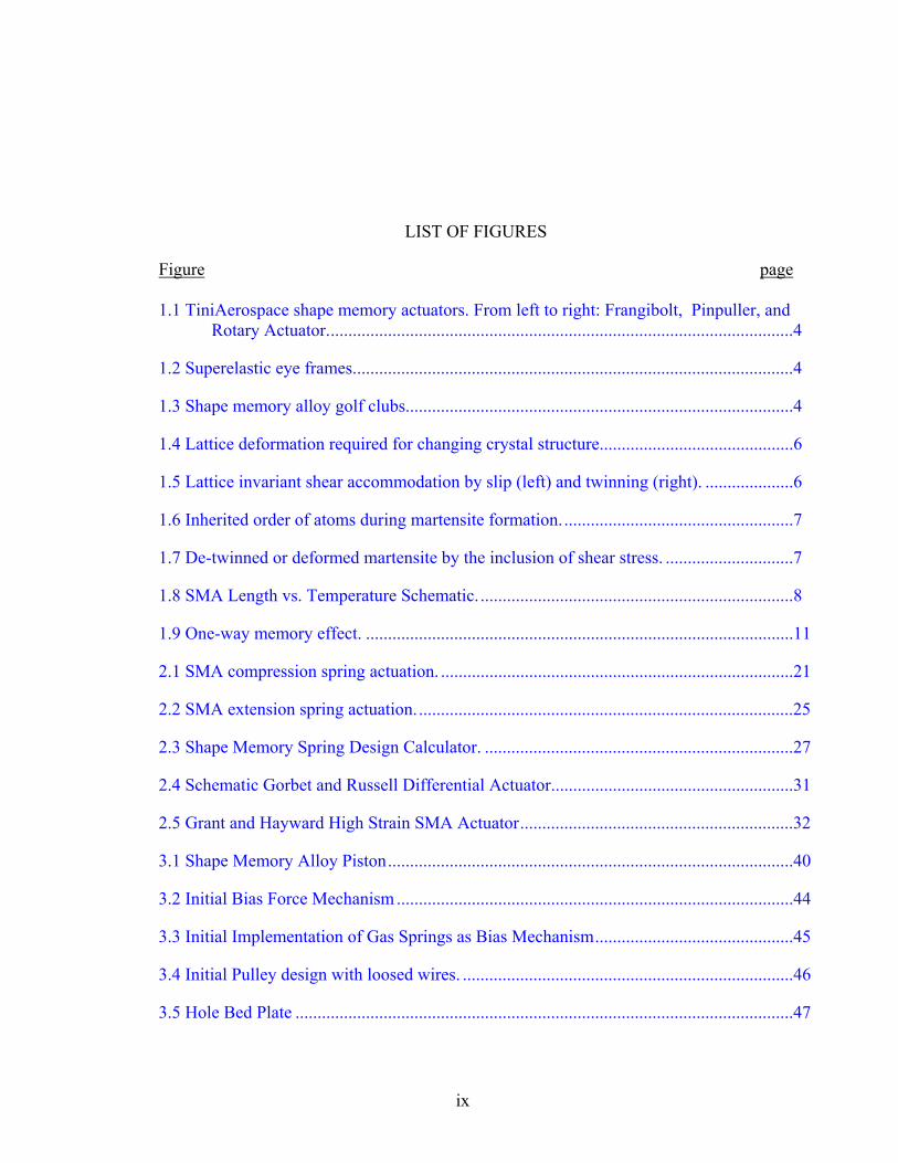
LIST OF FIGURES ........................................................................................................... ix
ABSTRACT....................................................................................................................... xi
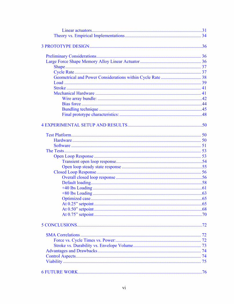
2 LITERATURE REVIEW ...............................................................................................16
Shape Setting Calculations ........................................................................................... 16 As Drawn Wire ...................................................................................................... 16 Strip or Ribbon Shape ............................................................................................ 18 Spring Shape .......................................................................................................... 20
Compression spring calculations .....................................................................20 Extension spring calculations ..........................................................................25 Shape memory alloy spring design calculator .................................................26
Special Forms......................................................................................................... 27 Activation Methods....................................................................................................... 28
Linear actuators................................................................................................31 Theory vs. Empirical Implementations .................................................................. 34
Preliminary Considerations........................................................................................... 36 Large Force Shape Memory Alloy Linear Actuator ..................................................... 36
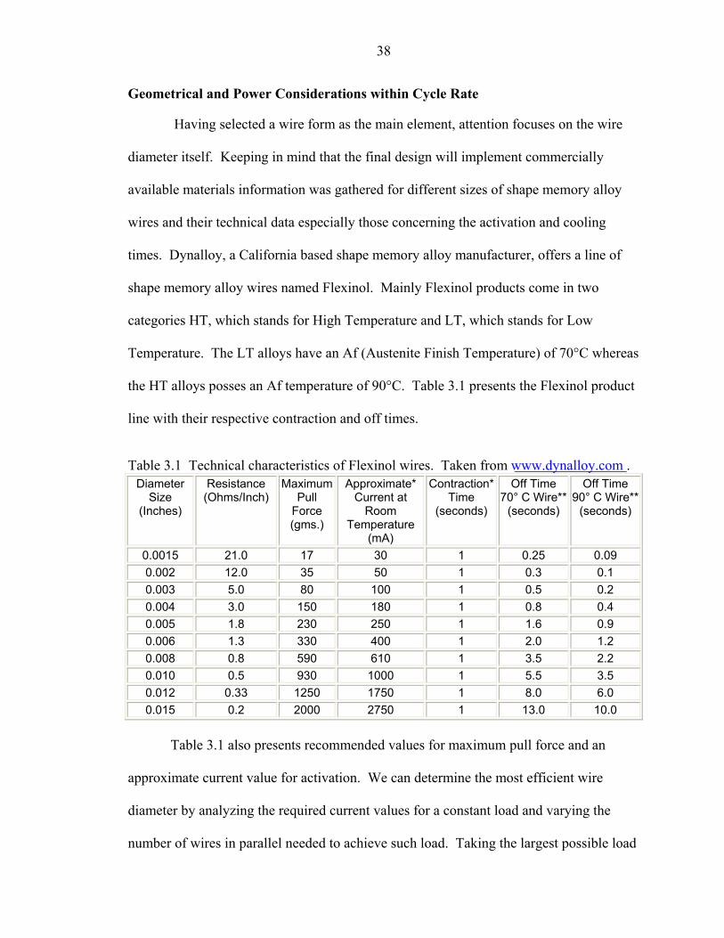
Shape...................................................................................................................... 37 Cycle Rate .............................................................................................................. 37 Geometrical and Power Considerations within Cycle Rate ................................... 38 Load ....................................................................................................................... 39 Stroke ..................................................................................................................... 41 Mechanical Hardware ............................................................................................ 41
Wire array bundle: ...........................................................................................42 Bias force .........................................................................................................44 Bundling technique ..........................................................................................45 Final prototype characteristics: ........................................................................48
4 EXPERIMENTAL SETUP AND RESULTS.................................................................50
Test Platform................................................................................................................. 50 Hardware ................................................................................................................ 50 Software ................................................................................................................. 51
The Tests....................................................................................................................... 53 Open Loop Response ............................................................................................. 53
Transient open loop response...........................................................................54 Open loop steady state response ......................................................................55
SMA Correlations ......................................................................................................... 72 Force vs. Cycle Times vs. Power:.......................................................................... 72 Stroke vs. Durability vs. Envelope Volume........................................................... 73
Advantages and Drawbacks.......................................................................................... 74 Control Aspects............................................................................................................. 74 Viability ........................................................................................................................ 75
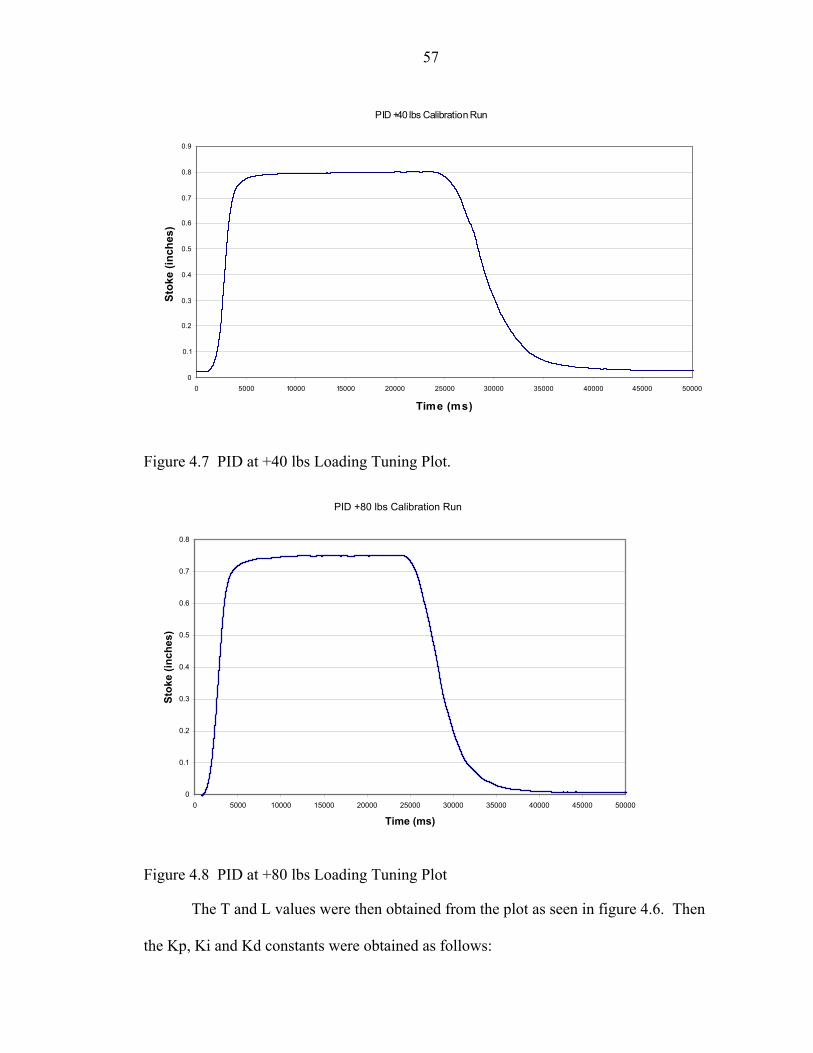
4.7 PID at +40 lbs Loading Tuning Plot. ...............................................................................57
4.8 PID at +80 lbs Loading Tuning Plot ................................................................................57
4.9 Overall Close Loop Response at Default Loading. .........................................................60
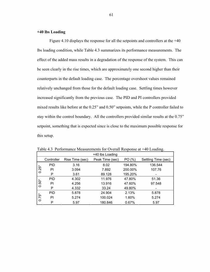
4.10 Overall Close Loop Response at +40 lbs Loading. ......................................................62
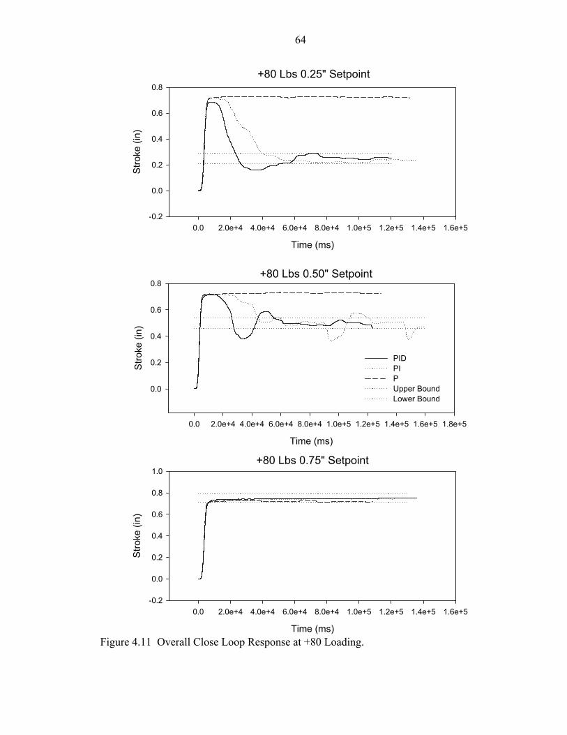
4.11 Overall Close Loop Response at +80 Loading. .............................................................64
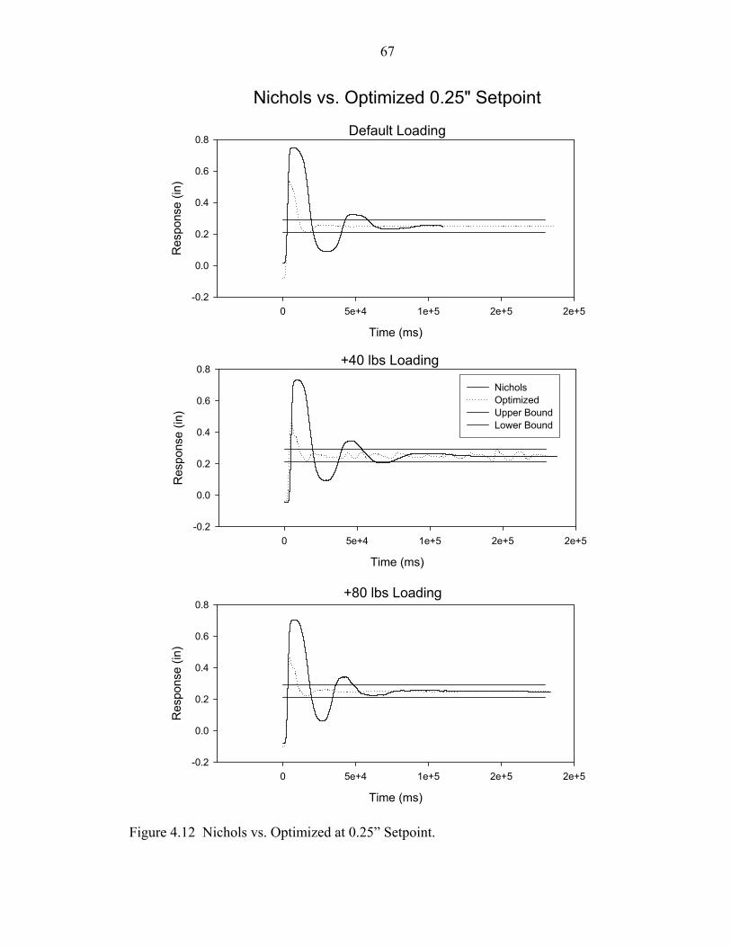
4.12 Nichols vs. Optimized at 0.25” Setpoint........................................................................67
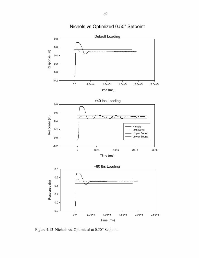
4.13 Nichols vs. Optimized at 0.50” Setpoint........................................................................69
xi
Abstract of Thesis Presented to the Graduate School
of the University of Florida in Partial Fulfillment of the Requirements for the Degree of Master of Science
LARGE FORCE SHAPE MEMORY ALLOY LINEAR ACTUATOR
By
José R. Santiago Anadón
August 2002
Chair: Dr. Carl D. Crane III Department: Mechanical Engineering
The design and development of a linear actuator for macro devices using shape
memory alloy (SMA) are desired. The implementation of shape memory alloys for large
scale applications has mainly three major drawbacks: strain constraints, limited cycles
and the actual usable force. This work will address two out of these three: the amount of
force and cycles. A parallel array of shape memory alloy wires working in unison was
implemented. The final prototype was capable of lifting more than 100 lbs with a stroke
of 0.80 inches. A PID controller was designed, implemented and tested for the actuator
and response data for different loading conditions, and setpoints were collected.
1
CHAPTER 1 INTRODUCTION
As technology advances, the building blocks that drive it remain relatively unchanged.
Motors, as were 100 years ago, are still being employed today as the preferred devices for
actuation and applications where the use of motors proves to be unpractical are in some
cases left behind or unexplored. In some instances a new revolutionary technology
comes along opening the door for new ideas and designs and with it, what seems
unfeasible in the past becomes now challenging. Think of all the engineering and science
problems that were thought of before the advent of computers and discarded because of
the intensive calculations that they required. Today we look at calculation intensive
problems on a daily basis and the main tool for solving them is the computer.
Although not as revolutionary as computers, shape memory alloys have proven their
worth in solving engineering problems that in the past seem implausible. Only a few
decades old, this new breed of driving mechanism has a bright future ahead. The main
reason behind their importance today is simple; shape memory elements provide a
significant amount of actuation with an extremely small envelope volume. This
statement becomes truer and their implementation even more important when looking at
the direction where technology is heading. In the modern world great emphasis has been
placed in miniaturization. Micro devices are being developed and implemented today to
perform a multitude of tasks with nano technology following very closely behind. These
machines can then be used for a multitude of applications such as robotics, biomechanics,
2
surgery, transportation vehicles, computer components, and recognizance and survey
devices.
Another advantage that shape memory alloys have over conventional actuation
mechanisms is their versatility. A shape memory element can be actuated thermally or
electrically. Not having to rely on moving parts for actuation, just the simple contraction
of the material, makes them highly attractive for actuation where low or no noise levels
are desired. Besides being an actuator they can also serve as thermal sensors and
superelastic springs. Some existing applications use them as an actuator and a sensory
device, thus minimizing space and cost for the designer. The most popular incarnation of
shape memory alloys, Ni-Ti, is biocompatible.
So far though, mainly because of efficiency concerns, shape memory alloys have yet
to be adopted fully in large-scale applications. Albeit that they do have a tough
competition with hydraulics, electrical motors, and internal combustion engines to go
against them, there are large-scale applications that would benefit from their use,
especially when size is a major design factor to consider. Although a complete chapter of
this work has been dedicated to these applications, a few of these applications are named
now to keep the scope of this research in context. The most logical application area for a
large-scale shape memory alloy actuator is biomechanics. A person that has lost an arm
for example can have a lightweight but incredibly powerful prosthesis without the need
of motors or compressors. Macro scale shape memory actuators can also be implemented
in situations where accessibility to the operation site is limited but when large amounts of
work are required. Aerospace is another field that benefits from these devices
3
minimizing the space and weight of a would-be actuator. In fact shape memory alloys
have already reached Mars as part of one of the mechanisms of NASA Mars Pathfinder.
This work focuses on the design and development of a large-scale shape memory
linear actuator. A design procedure was created which takes into account all the
correlations that exist in the design parameters and actuator properties. This procedure
serves as the basis for the development of the final prototype. Several prototypes were
designed; each one with a different approach as to the implementation of the shape
memory elements and one of these prototypes was built and tested.
Shape Memory Basics
The basics of memory materials have been extensively documented by numerous
papers and it is not the intention of this research to expand on this area, but rather than to
give the reader a primer into the subject to better understand latter topics.
The term shape memory alloy indicates a material that has the ability to deform to
a preset shape when heated and in the process perform a useful engineering function.
There are five documented functions that a SMA can deliver [1]:
1. Free recovery describes a SMA element whose sole function is to cause a displacement. Since no work is being produced this kind of application is mostly used in control devices and relay mechanisms.
2. In constrained recovery the element is prevented from displacement generating large amount of stresses. This type of function is being used increasingly in fittings, couplings and connectors for machinery.
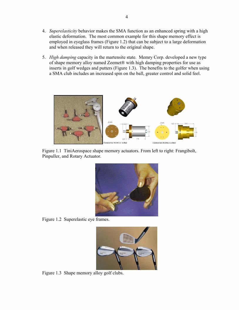
3. When used as an Actuator, the SMA element produces work that is force coupled with displacement. A vast majority of applications employ SMA in this fashion. Tini Aerospace has had great success developing shape memory actuators for space applications. Currently the company offers three major actuators (Figure 1.1): The Frangibolt actuator uses a SMA cylinder to elongate and in the process fracture a bolting element with forces up to 5000 lbf, which upon release deploys a structure. The other two actuators provide linear and rotational motion.
4
4. Superelasticity behavior makes the SMA function as an enhanced spring with a high elastic deformation. The most common example for this shape memory effect is employed in eyeglass frames (Figure 1.2) that can be subject to a large deformation and when released they will return to the original shape.
5. High damping capacity in the martensite state. Memry Corp. developed a new type of shape memory alloy named Zeemet® with high damping properties for use as inserts in golf wedges and putters (Figure 1.3). The benefits to the golfer when using a SMA club includes an increased spin on the ball, greater control and solid feel.
Figure 1.1 TiniAerospace shape memory actuators. From left to right: Frangibolt, Pinpuller, and Rotary Actuator.
Figure 1.2 Superelastic eye frames.
Figure 1.3 Shape memory alloy golf clubs.
5
Martensitic Transformations
In general, the shape memory event is based on the ability of the material to
change its crystal structure, in other words transforming from one crystal structure to
another. In shape memory alloys this transformation is usually referred to as a
martensitic transformation. The term martensite takes its name from Adolf Martens
(1850-1914) a German metallurgist who first discovered this structure in steels. Later it
was discovered that this transformation between austenite and martensite phases was not
limited to steel [2].
When a material changes phase the rearranging of atoms that takes place is
referred to as a transformation. In solids there are two known types of transformations:
displacive and diffusional. In a diffusional transformation the rearranging of atoms
occurs across long distances. The new phase formed by a diffusional transformation is of
different chemical composition than that of the parent phase. In contrast, a displacive
transformation occurs by the movement of atoms as a unit, with each atom contributing a
small portion of the overall displacement. In a displacive transformation the bonds
between the atoms are not broken rather than arranged, thus leaving the parent phase
chemical composition matrix intact. Martensitic transformations in shape memory alloys
are of displacive type and transformation takes place between Austenite also usually
referred to as the parent phase and Martensite. Duerig et al. [3] categorizes the austenite
to martensite transformation into two parts: Bain Strain and lattice-invariant shear. The
Bain Strain takes its name from Bain who in 1924 proposed it and refers to the necessary
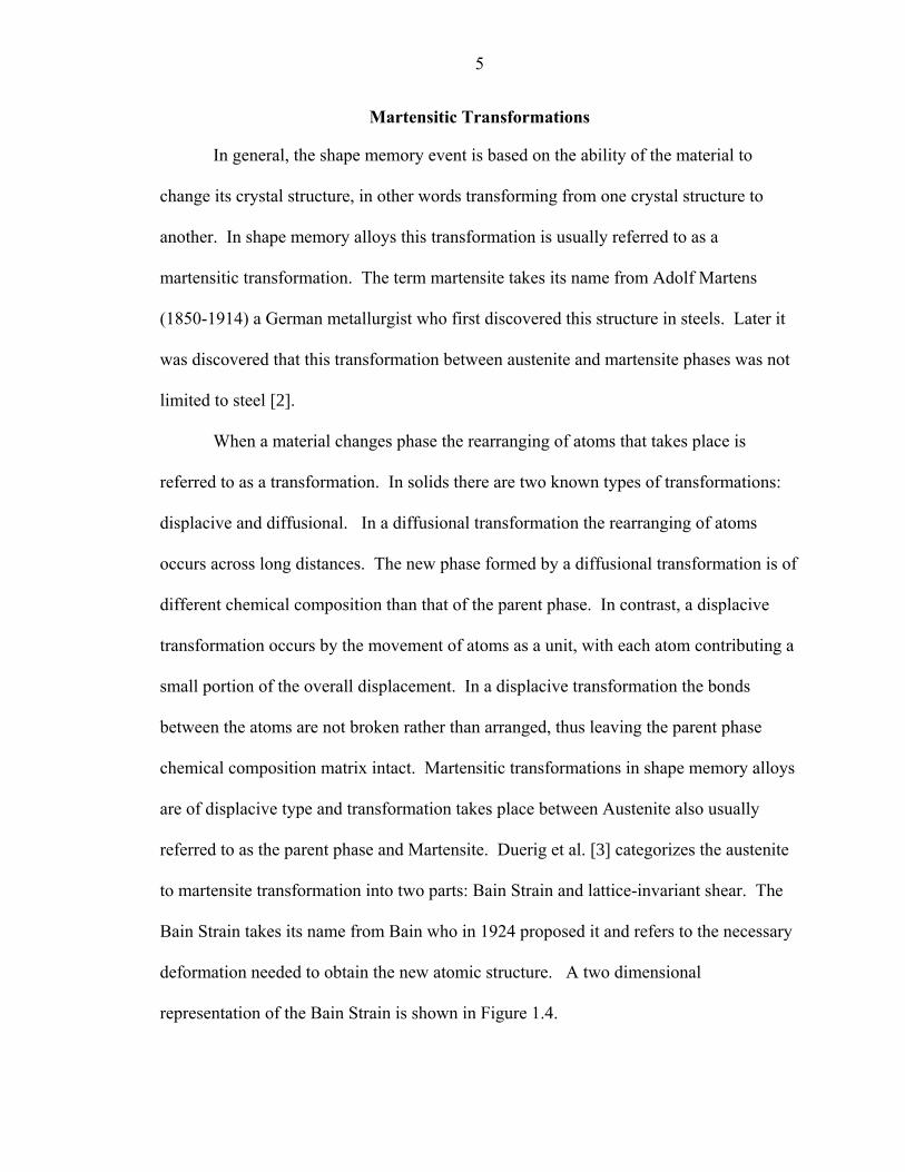
deformation needed to obtain the new atomic structure. A two dimensional
representation of the Bain Strain is shown in Figure 1.4.
6
Figure 1-4 Lattice deformation required for changing crystal structure.
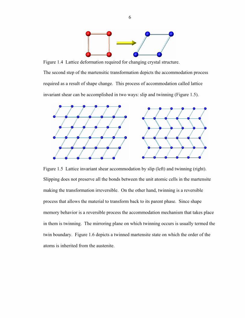
The second step of the martensitic transformation depicts the accommodation process
required as a result of shape change. This process of accommodation called lattice
invariant shear can be accomplished in two ways: slip and twinning (Figure 1.5).
Figure 1.5 Lattice invariant shear accommodation by slip (left) and twinning (right).
Slipping does not preserve all the bonds between the unit atomic cells in the martensite
making the transformation irreversible. On the other hand, twinning is a reversible
process that allows the material to transform back to its parent phase. Since shape
memory behavior is a reversible process the accommodation mechanism that takes place
in them is twinning. The mirroring plane on which twinning occurs is usually termed the
twin boundary. Figure 1.6 depicts a twinned martensite state on which the order of the
atoms is inherited from the austenite. Since twin boundaries can be readily moved, the
inclusion of an external shear stress can alter the twinned martensitic state of the matrix
to reflect only one variant of twinning as shown on Figure 1.7.
Although the previous review introduces the reader to the shape memory
7
Figure 1.6 Inherited order of atoms during martensite formation.
Figure 1.7 De-twinned or deformed martensite by the inclusion of shear stress.
internals, it does not tell the entire picture. In practical terms the behavior mentioned
above is related to the temperature of the shape memory element, which determines its
crystallographic state. A typical shape memory element has four relevant temperatures
that define the different stages of actuation, thus providing the designer a method for
control. Simply put, the four temperatures define the start and finish transformations for
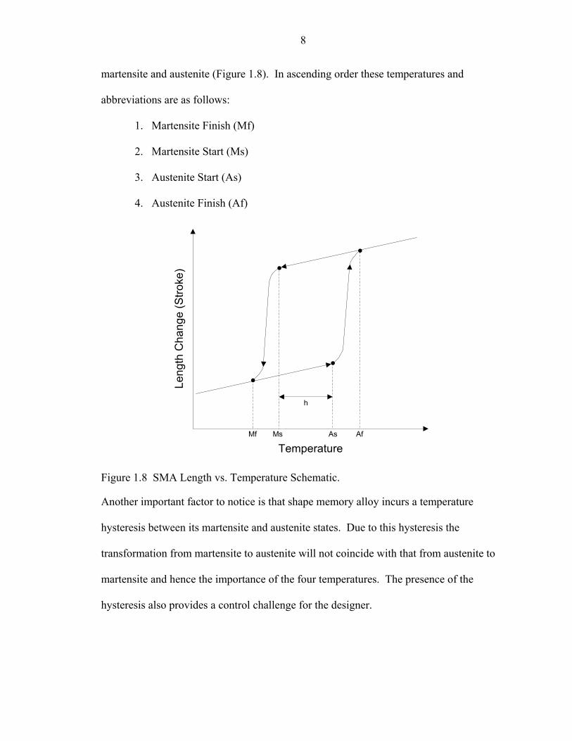
martensite and austenite (Figure 1.8). In ascending order these temperatures and
abbreviations are as follows:
1. Martensite Finish (Mf)
2. Martensite Start (Ms)
3. Austenite Start (As)
4. Austenite Finish (Af)
8
TemperatureMf AfAsMs
Leng
th C
hang
e (S
troke
)
h
Figure 1.8 SMA Length vs. Temperature Schematic.
Another important factor to notice is that shape memory alloy incurs a temperature
hysteresis between its martensite and austenite states. Due to this hysteresis the
transformation from martensite to austenite will not coincide with that from austenite to
martensite and hence the importance of the four temperatures. The presence of the
hysteresis also provides a control challenge for the designer.
The Shape Memory Effect
In order for an alloy to exhibit shape memory behavior certain conditions must be met.
Specific weight percentages of each element must be combined in a precise fashion to
produce a shape memory viable material. Additional processes enhance material
properties and define their shape setting characteristics. Depending on the processing
technique used a shape memory element can display one of five distinct shape memory
behaviors. These effects are discussed next.
9
One-Way Memory
This is the most basic form of shape memory and hence the most adopted due to
the lower amount of processing that goes into the material, which translates to a reduced
cost. This type of effect can be described by its operation cycle outlined below.
A shape memory as-drawn wire initially in its martensite phase has a temperature
equal or lower than the martensite finish temperature (Mf). Microscopically the element
will have the material martensitic unit atomic structure1 and an untwinned or deformed
matrix structure; macroscopically the element will be in its relaxed state. If the
temperature of the element is gradually raised at some point austenite will begin to form
in the element, hence the name austenite start temperature (As). Austenitic structures
will begin appearing in the once fully martensite and as the temperature raises the
percentage of austenite will increase as well. Physically the wire will start to compress
and if designed for, produce work. The austenite finish temperature marks the end of the
austenitic transformation. At this point the matrix is fully of austenitic atomic structure
and a wire with a reduced length should be noticed. The material temperature is now
lowered until it reaches the temperature known as martensite finish (Mf). In the same
way as austenite before, the material will start reverting to its martensite state. The
orientation of the martensite crystals will be in a twinned fashion with an inherited order
from the austenite and multiple variations as to accommodate whatever volume the
austenite once occupied. Eventually the element will cool furthermore until it reaches the
Martensite Finish temperature (Mf) again. Despite the fact that the material completed a
1 Shape memory alloys atomic structures can vary greatly. For purposes of simplification the schematics presented in this work are assumed as cubic for austenite state and rhombohedral for martensite.
10
full cycle, at least temperature-wise, a full actuation cycle requires a reset force to deform
the martensite back to a uniform favored variant of atomic structure and an untwinned
martensite state. If no reset force is applied during the cooling process, the shape of the
material will not change and is only the inclusion of this force that an observable
elongation in the wire should be noted. Once the untwinned martensite has been forced
the cycle can begin again.
The bias force will also gradually decrease as the actuator performs more cycles.
The general concept behind this behavior, termed walking, relies on the ability of the
material to also remember its martensitic deformed state. Walking is a form of the next
memory effect to be discussed called two-way memory with the only difference being
that the material learns the behavior during processing instead of operation.
Two-Way Memory
On a two-way memory actuator the inclusion of the external stress can be lowered
and in some cases not needed at all due to the fact that the alloy will, upon reaching Mf,
revert to its original deformed martensite shape. In two-way systems the amount of work
that the alloy is capable of producing during the falling cycle (martensite transformation)
is minimal and no loading is recommended at this stage. In fact this type of memory
setting is only used to reduce or dismiss the biasing force completely. Perkins and
Hodgson [4] describe this effect in more detail and give processing methods on how to
obtain alloys that will exhibit the two-way effect. Ryhänen [5] describes two methods for
obtaining two-way memory.
All Around Memory Effect
Depending on the composition and processing of the alloy a special case of two-
way memory has been found and termed all-around memory effect. The most telling
11
Tem
pera
ture
Mf
Af
As
Ms
Length
h
1
Mf
TM
arte
nsite
Def
orm
ed≤
_
3
AfTAu
sten
ite≥
5
Mf
TM
arte
nsite
Twin
ned
≤_
2
AfT
AsAu
sten
iteM
arte
nsite <
<−
4
Mf
TM
sM
arte
nsite
Aust
enite >
>−
Stroke
Figu
re 1
.9 O
ne w
ay sh
ape
mem
ory
effe
ct.
12
feature of this type of memory is that the low and high temperature shapes are complete
opposites. Perkins and Hodgson also describe this effect in more detail [4]. The
following was taken from Shape Memory Alloys [2] on which Funabuko gives a general
technique for obtaining this type of memory effect for binary Ni-Ti:
1. Deform the martensite beyond the limit.
2. Deform the parent phase more than is possible in a stress induced martensite transformation.
3. Deform the parent phase, cool the specimen to below the Mf temperature under restriction, and maintain this under stress for a long period of time.
4. Deform the martensite phase, heat the specimen under restriction, and induce the reverse transformation.
5. Deform the specimen after creating minute precipitates in the parent phase.
R-Phase Transformation
Besides the martensite - austenite transformation there exists one more noticeable
transformation in shape memory alloys. When an alloy is cooled down from Af the
material can transform from an austenite cubic to a rhombohedral lattice structure, which
is why the name R-Phase transformation. The most noticeable drawback of using this
type of transition is that the strain associated with this transformation is rather small, only
0.5%. The temperature hysteresis can be as low as 1.5°C and that makes them ideal for
high cycle rate thermally controlled actuators. It has been proved that these kinds of
actuators suffer less from fatigue and can yield millions of cycles before failing or
degrading. Several researchers have described this effect in more detail including Otsuka
[6] and Suzuki and Tamura [7], who describe the fatigue properties.
13
Superelasticity
Every one of the shape memory effects described above requires a temperature
change to precipitate the transformation. There exists, however, a special memory effect
under which no temperature change is needed called superelasticity. When
superelasticity is present in a SMA the martensite state is induced by an external applied
stress. When the stress is released the material reverts back to its austenite state. For the
material to exhibit superelasticity it must be designed to have an Austenite finish
temperature near the operating temperature, this in most cases would be ambient. Duerig
and Zadno [8] explain this effect in more detail.
Shape Memory Materials
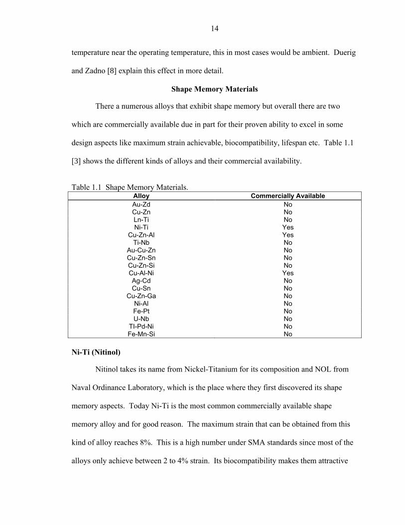
There a numerous alloys that exhibit shape memory but overall there are two
which are commercially available due in part for their proven ability to excel in some
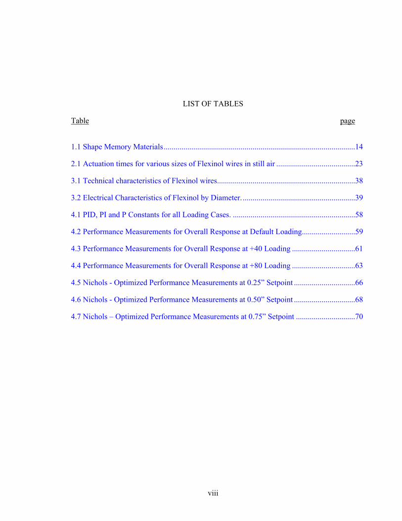
design aspects like maximum strain achievable, biocompatibility, lifespan etc. Table 1.1
[3] shows the different kinds of alloys and their commercial availability.
Table 1.1. Shape Memory Materials. Alloy Commercially Available Au-Zd No Cu-Zn No Ln-Ti No Ni-Ti Yes
Cu-Zn-Al Yes Ti-Nb No
Au-Cu-Zn No Cu-Zn-Sn No Cu-Zn-Si No Cu-Al-Ni Yes Ag-Cd No Cu-Sn No
Cu-Zn-Ga No Ni-Al No Fe-Pt No U-Nb No
TI-Pd-Ni No Fe-Mn-Si No
14
Ni-Ti (Nitinol)
Nitinol takes its name from Nickel-Titanium for its composition and NOL from
Naval Ordinance Laboratory, which is the place where they first discovered its shape
memory aspects. Today Ni-Ti is the most common commercially available shape
memory alloy and for good reason. The maximum strain that can be obtained from this
kind of alloy reaches 8%. This is a high number under SMA standards since most of the
alloys only achieve between 2 to 4% strain. Its biocompatibility makes them attractive
for medical applications. The only drawback lies on its cost, which is substantially
higher than its peers.
Ni-Ti-Cu
Although Ni-Ti is the most common standard shape memory alloy available some
of its properties might not be adept for specific designs. Because of this, extensive
research has been conducted to improve some of its mechanical properties. One of the
methods of doing this is by adding a ternary element to Ni-Ti. Cu addition to Ni-Ti
lowers the martensite phase yield strength of the material and produces a smaller
temperature hysteresis when compared to Ni-Ti. Lower yield strength on the martensite
phase will decrease the amount of bias force required to deform the SMA element in that
phase thus providing a higher net output force. The smaller temperature hysteresis
provides faster actuation times or cycle rates, it can also make the actuator more suitable
for thermal actuation.
15
CHAPTER 2 LITERATURE REVIEW
The nature of shape memory design requires that the designer have a vast
understanding of the subject. The role of this review is twofold: to provide the user with
common accepted background and computational procedures that relate to shape memory
design and a review of current devices similar to the one proposed.
Shape Setting Calculations
One of the main advantages of using shape memory alloys is the fact that they can
be set to take any form the designer imparts on them. In reality because of the cost of
shape setting and the limitations in force and stroke, non-conventional shapes are not
used very often. Instead more conventional, mass produced shapes are usually employed.
The most common of the conventional shapes are wire, ribbon or strip, and springs. This
section will discuss these shapes in more detail and review accepted design
methodologies.
As Drawn Wire
Wire is the most common form of shape memory alloy. When compared to
other forms it provides the maximum amount of force per cross sectional area, matched
only by strip or ribbon form. The design methodology for wire actuator is documented in
Tom Waram’s Actuator Design Using Shape Memory Alloys [9]. His approach assumes
a linear stress strain behavior of the alloy in the operational temperature range (Mf – Af).
Another assumption is that the given design parameters are only force and stroke. The
actuator force and diameter are related by the stress:
16
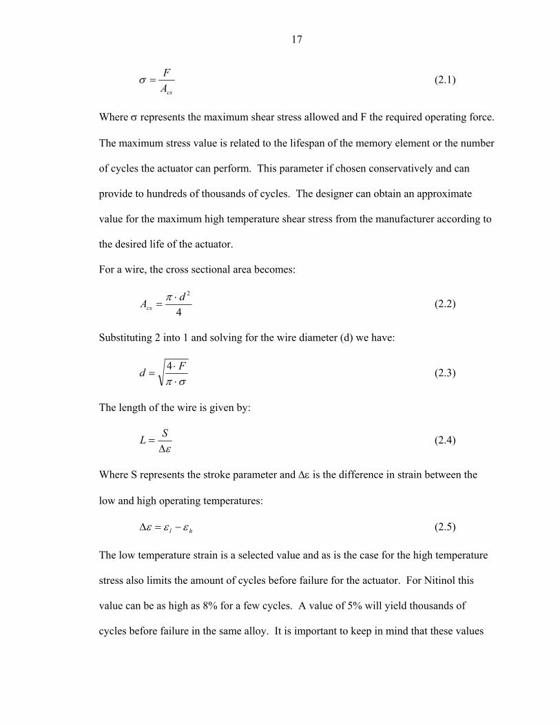
csAF
=σ (2.1)
Where σ represents the maximum shear stress allowed and F the required operating force.
The maximum stress value is related to the lifespan of the memory element or the number
of cycles the actuator can perform. This parameter if chosen conservatively and can
provide to hundreds of thousands of cycles. The designer can obtain an approximate
value for the maximum high temperature shear stress from the manufacturer according to
the desired life of the actuator.
For a wire, the cross sectional area becomes:
4
2dAcs⋅
=π (2.2)
Substituting 2 into 1 and solving for the wire diameter (d) we have:
σπ ⋅⋅
=Fd 4 (2.3)
The length of the wire is given by:
ε∆=
SL (2.4)
Where S represents the stroke parameter and ∆ε is the difference in strain between the
low and high operating temperatures:
hl εεε −=∆ (2.5)
The low temperature strain is a selected value and as is the case for the high temperature
stress also limits the amount of cycles before failure for the actuator. For Nitinol this
value can be as high as 8% for a few cycles. A value of 5% will yield thousands of
cycles before failure in the same alloy. It is important to keep in mind that these values
17
are dependant in the type of alloy implemented since using the same values in Ni-Ti-Cu
for example would yield far less cycles. From Hooke’s Law we can obtain the high
temperature strain:
h
hh E
σε = (2.6)
where Eh is the Young Modulus of the Material at the high temperature. The length
increment of the wire at the high temperature becomes:
LL hi ⋅= ε (2.7)
where Li is the length increment and L is the total length of the element. Using the
Young Modulus definition once again but this time in the low temperature range and
solving for the low temperature shear stress gives us:
lll E⋅= εσ (2.8)
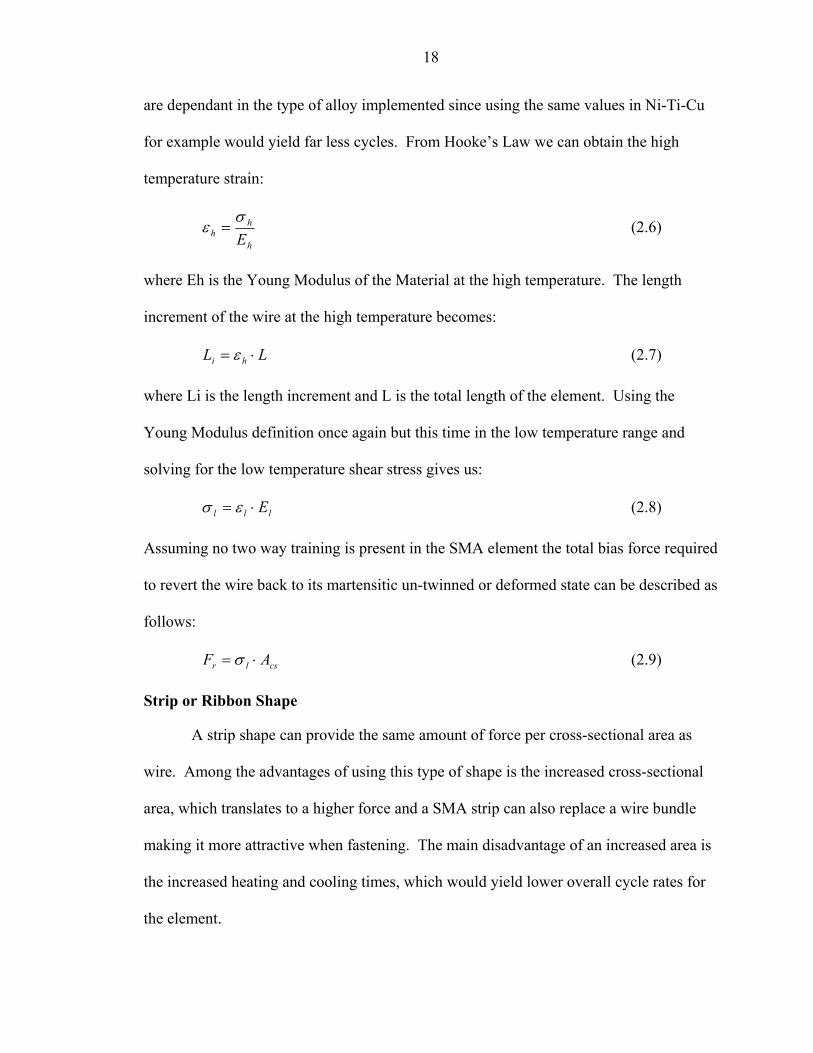
Assuming no two way training is present in the SMA element the total bias force required
to revert the wire back to its martensitic un-twinned or deformed state can be described as
follows:
cslr AF ⋅= σ (2.9)
Strip or Ribbon Shape
A strip shape can provide the same amount of force per cross-sectional area as
wire. Among the advantages of using this type of shape is the increased cross-sectional
area, which translates to a higher force and a SMA strip can also replace a wire bundle
making it more attractive when fastening. The main disadvantage of an increased area is
the increased heating and cooling times, which would yield lower overall cycle rates for
the element.
18
Calculation for this type of shape follows that of wire with the only difference
being the element area:
hwAcs ⋅= (2.10)
The dimensions in the strip element are related by:
hwR hw =− (2.11)
Rw-h represents the strip’s width to height ratio. This number is restricted by the
processing capabilities of the manufacturer with typical values ranging from 10 to 15.
Ideally the maximum possible width-height ratio will yield the lowest height for the same
area. The advantage to having small height relates to a high heat transfer rate between
the SMA element and its environment. Another factor affected by the shape memory
height is the minimum bend radius. When a SMA is bent the stresses at the surface area
of the bent region will be higher than the rest of it. As a result the life of the element can
be considerably reduced. Gilbertson [10] recommends the minimum bend radius for a
wire to be:
dr ⋅= 50min (2.12)
In the previous equation d represents the wire diameter and rmin is the minimum bend
radius. For strip this value is fifty times the height:
hr ⋅= 50min (2.13)
Designing for the lowest possible height, the strip area becomes:
2hRA hwcs ⋅= − (2.14)
Substituting 2.14 into 2.1 and solving for h yields:
19
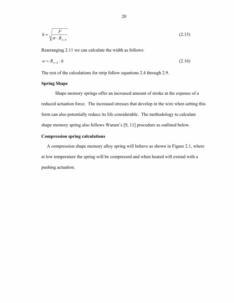
hwRFh
−⋅=
σ (2.15)
Rearranging 2.11 we can calculate the width as follows:
hRw hw ⋅= − (2.16)
The rest of the calculations for strip follow equations 2.4 through 2.9.
Spring Shape
Shape memory springs offer an increased amount of stroke at the expense of a
reduced actuation force. The increased stresses that develop in the wire when setting this
form can also potentially reduce its life considerable. The methodology to calculate
shape memory spring also follows Waram’s [9, 11] procedure as outlined below.
Compression spring calculations
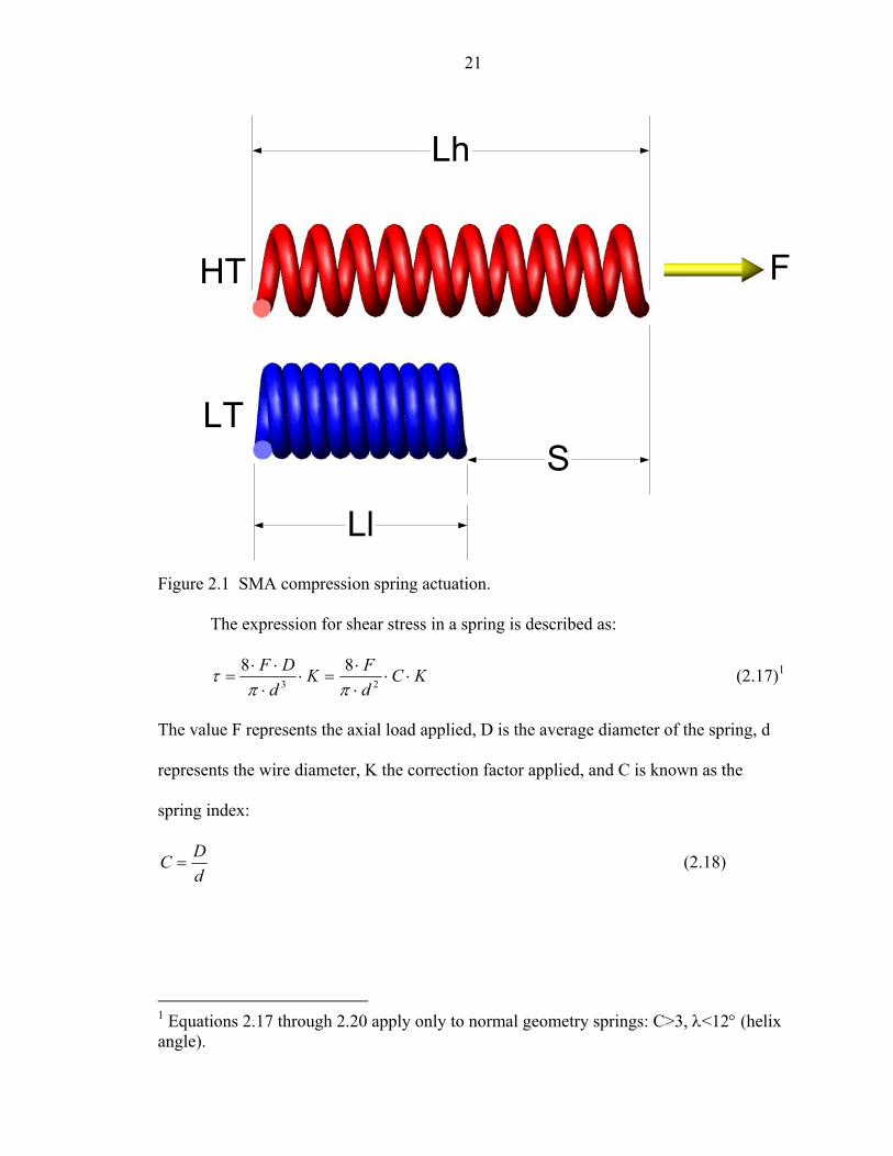
A compression shape memory alloy spring will behave as shown in Figure 2.1, where
at low temperature the spring will be compressed and when heated will extend with a
pushing actuation.
F
S
Lh
Ll
LT
HT
Figure 2.1. SMA compression spring actuation.
20
The expression for shear stress in a spring is described as:
KCdFK
dDF
⋅⋅⋅⋅
=⋅⋅⋅⋅
= 23
88ππ
τ (2.17)1
The value F represents the axial load applied, D is the average diameter of the spring, d
represents the wire diameter, K the correction factor applied, and C is known as the
spring index:
dDC = (2.18)
With the exemption of the K factor, equation 2.17 is the torsional stress for a solid round
bar. The K value, also know as Wahl correction factor, corrects this shear stress to
account for transverse and torsional shear stresses present in a spring:
CCCK w
615.04414+
−⋅−⋅
= (2.19)
Juvinall and Marshek [12] recommend the use of equation 2.19 for fatigue loading
whereas equation 2.20 is often used for static loading only:
CK s
5.01+= (2.20)
Because of fatigue limitations in shape memory alloys the shear stress in 2.17 must be set
by the designer to a value that would yield the desired life for the actuator2. From
equation 2.17 we can obtain multiple wire diameters for the actuator for acceptable
values of C ranging from 3 to 12:
1 Equations 2.17 through 2.20 apply only to normal geometry springs: C>3, λ<12° (helix angle). 2 The maximum shear stress depends heavily on the type of alloy used. Estimate values for 100,000 cycles for Ni-Ti and Ni-Ti-Cu are 170 Mpa and 140 Mpa respectively.
21
τπ ⋅⋅⋅⋅
=KCFd 8 (2.21)
There are two factors that relate to the value of C in the design specifications: the cycle
rate and the envelope volume of the actuator. Since the cycle rate is a function of the
wire diameter, a value of C can be selected to accommodate a desired cycle rate. Shape
memory alloy manufacturers usually provide actuation timetables for different wire
diameters as shown in Table 2.1.
Table 2.1. Actuation times for various sizes of Flexinol wires in still air [11]. Name Flexinol 025 Flexinol 050 Flexinol 100 Flexinol 150 Flexinol 250 Diameter (µm) 25 50 100 150 250 Max. Contraction Speed (sec)
0.1 0.1 0.1 0.1 0.1
Relaxation Speed (sec)
0.1 0.3 0.8 2 5.5
Typical Cycle Rate
55 46 33 20 9
The other method for setting the C value depends on the envelope volume of the actuator
that depends on the spring outer diameter and length, which will be discussed next.
The average diameter of the spring can be obtained from 2.18 solving for D:
dcD ⋅= (2.22)
The outer and inner diameters can be obtained from equations 2.23 and 2.24:
dDOD += (2.23)
dDID −= (2.24)
The number of turns in the spring can be obtained from:
γπγπ ∆⋅⋅⋅=
∆⋅⋅⋅
=CD
SD
Sdn 2 (2.25)
Where S represents the stroke of the actuator, and ∆γ the strain difference at high and low
temperatures:
22
hl γγγ −=∆ (2.26)
The low temperature shear strain also affects the overall life of the actuator and must be
set to a reasonable value. The high temperature shear strain can be obtained from the
stress strain material chart for the assumed high temperature shear stress. Another
method for estimating this value is by assuming a linear stress-strain behavior in which
case the high temperature shear strain can be evaluated from the high temperature shear
stress, τh and shear modulus, Gh:
h
hh G
τγ = (2.27)
The spring rate for the high and low temperature ranges can be evaluated as
follows:
33
4
88 CndG
DndGk hh
h ⋅⋅⋅
=⋅⋅⋅
= (2.28)
33
4
88 CndG
DndGk ll
l ⋅⋅⋅
=⋅⋅⋅
= (2.29)
With the spring rate we can evaluate the high temperature spring deflection as:
hh k
F=δ (2.30)
Since the stroke is the difference between the low and high temperature spring
deflections we can derive the low temperature deflection from that as follows:
hl S δδ += (2.31)
At low temperature the spring will be compressed with a length described by:
)3( +⋅= ndLl (2.32)
At the high temperature the spring will actuate to a length of:
23
SLL lh += (2.33)
The free length of the spring will be:
hhf LL δ+= (2.34)
For one-way memory springs the required force to revert the shape memory alloy to its
deformed martensite is given as:
llr kF δ⋅= (2.35)
The envelope volume of the spring can be evaluated from the occupied area and height:
4
2ODAe⋅
=π (2.36)
fe LODV ⋅⋅
=4
2π (2.37)
If designing for an effective envelope volume an iteration process is recommended at this
point to evaluate the best value for the spring index.
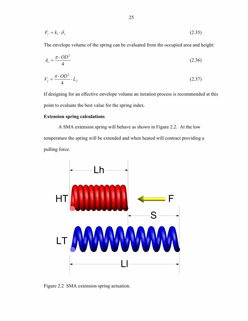
Extension spring calculations
A SMA extension spring will behave as shown in Figure 2.2. At the low
temperature the spring will be extended and when heated will contract providing a
pulling force.
F
S
Ll
Lh
LT
HT
Figure 2.2. SMA extension spring actuation.
24
With the exception of the spring lengths the equations from the previous section
can be used to determine the spring diameters, number of turns, spring rates and reset
force. Since the actuation for a spring working in extension is reversed from that in
compression the lengths must be reevaluated. The spring body length describes a fully
compressed spring:
)1( +⋅= ndLb (2.38)
Where n is the number of turns of the spring. The free length of the spring or the length
at which the shape setting takes place can now be evaluated as a function of the body
length:
IDLL bf ⋅+= 2 (2.39)
When heated the spring will have a length of:
hfh LL δ+= (2.40)
Since the stroke must be equal to the difference of the high and low temperature lengths
the low temperature length can be calculated as:
SLL hl += (2.41)
where S is the stroke.
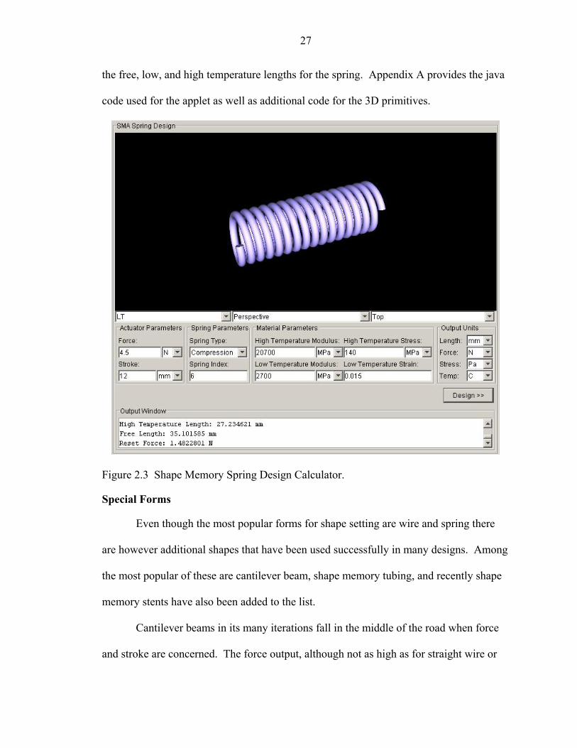
Shape memory alloy spring design calculator
During the course of this research a spring actuator was considered as one of the
possible final prototypes. For this endeavor an applet was created to help in calculating
the design characteristics of SMA springs. Figure 2.3 shows a screenshot of the applet,
which can be found at http://plaza.ufl.edu/jrsan/smad-main.htm. The java based applet
takes as input all the variables found in the spring calculations shown on the previous
sections and outputs a 3D rendered model of the spring the user has the ability to view
25
the free, low, and high temperature lengths for the spring. Appendix A provides the java
code used for the applet as well as additional code for the 3D primitives.
Figure 2.3. Shape Memory Spring Design Calculator.
Special Forms
Even though the most popular forms for shape setting are wire and spring there
are however additional shapes that have been used successfully in many designs. Among
the most popular of these are cantilever beam, shape memory tubing, and recently shape
memory stents have also been added to the list.
Cantilever beams in its many iterations fall in the middle of the road when force
and stroke are concerned. The force output, although not as high as for straight wire or
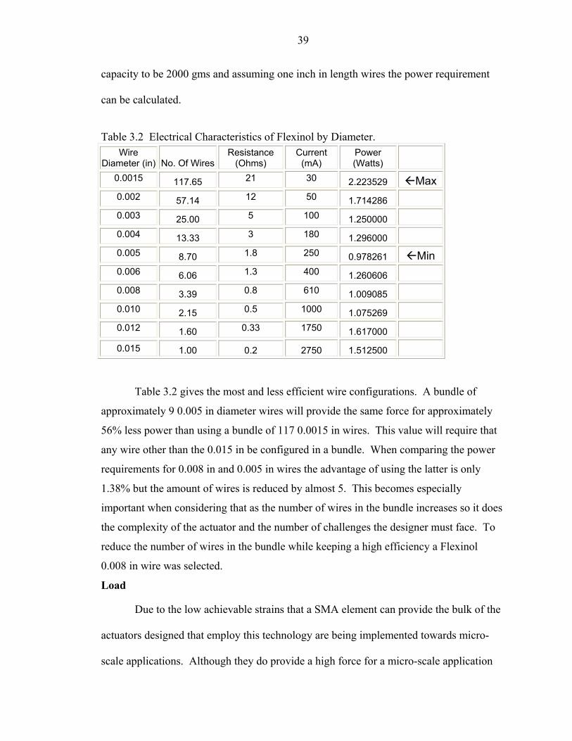
Table 3.2 gives the most and less efficient wire configurations. A bundle of
approximately 9 0.005 in diameter wires will provide the same force for approximately
56% less power than using a bundle of 117 0.0015 in wires. This value will require that
any wire other than the 0.015 in be configured in a bundle. When comparing the power
requirements for 0.008 in and 0.005 in wires the advantage of using the latter is only
1.38% but the amount of wires is reduced by almost 5. This becomes especially
important when considering that as the number of wires in the bundle increases so it does
the complexity of the actuator and the number of challenges the designer must face. To
reduce the number of wires in the bundle while keeping a high efficiency a Flexinol
0.008 in wire was selected.
Load
Due to the low achievable strains that a SMA element can provide the bulk of the
actuators designed that employ this technology are being implemented towards micro-
scale applications. Although they do provide a high force for a micro-scale application
37
the actual load pales when compared to the macro application loads. To put the loading
parameter in context we must first consider micro-scale loading. Take for example one
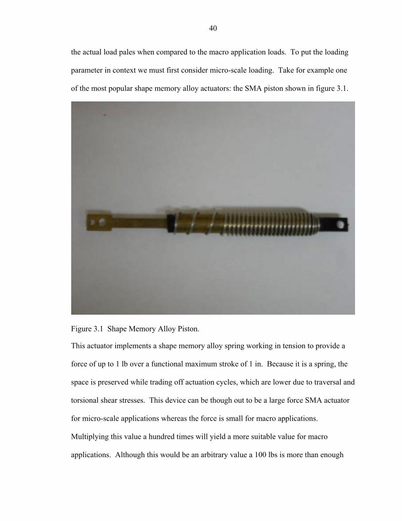
of the most popular shape memory alloy actuators: the SMA piston shown in figure 3.1.
Figure 3.1. Shape Memory Alloy Piston.
This actuator implements a shape memory alloy spring working in tension to provide a
force of up to 1 lb over a functional maximum stroke of 1 in. Because it is a spring, the
space is preserved while trading off actuation cycles, which are lower due to traversal and
torsional shear stresses. This device can be though out to be a large force SMA actuator
for micro-scale applications whereas the force is small for macro applications.
Multiplying this value a hundred times will yield a more suitable value for macro
applications. Although this would be an arbitrary value a 100 lbs is more than enough
number to claim the actuator as suitable for macro applications in the loading realm.
Shape memory alloy actuators that have been developed in the past as claiming to be
large force posses loading values of up to 20 pounds; this would mean that an actuator
with 5 times the capacity of this one would also fit this description.
38
Stroke
Although the purpose of the actuator to be designed is only for large force, the
stroke must posses a reasonable value that would give some room for the implementation
of control. Too small of a stroke would make the actuator virtually impossible to control
since small increments in current transform to big movements. Another factor that
dominates this parameter is the hysteresis associated with the shape memory element.
Since the actuation temperatures (As to Af) are different than the cooling ones (Ms to
Mf) this makes the modulation range of the actuator a higher value than with purely
linear systems. Overall a value of 1 in was selected having the actuator work on average
between 4 to 5 percent strain thus ensuring hundreds of thousands of cycles.
Mechanical Hardware
Based on the selected shape memory elements a linear actuator was designed and
implemented. The following is the design criteria used for the resulting actuator:
1. A parallel configuration will account for the smaller, faster elements while providing a large force when working together.
2. Serviceability must be kept manageable.
3. Versatility will allow interchanging the shape memory alloy elements for other wires and thus serving as a testing platform for current and upcoming shape memory alloy wire and ribbon technologies.
4. Reset and tensioning devices must be implemented to ensure that no loss stroke is wasted and to allow for faster response. The reset mechanism will also provide a bias force so that the actuator is always ready to be activated.
5. Electrical connections must enforce that a uniform current passes through each wire.
The following section will discuss these points in more detail while observing the
preliminary and final design implementations.
39
Wire array bundle:
The implementation of an array bundle provides a simple solution to multiple
problems. When correctly implemented an array configuration must address the
following:
1. The array must be able to maintain a uniform tension across all the wires.
2. The configuration must ensure that uniform current flows through all the elements in the array.
3. A parallel array should provide for lower response times by implementing faster elements.
The main purpose for the use of an array is to provide faster actuation while
maintaining a large uniform force. The reasoning behind this is rather simple, actuation
times is directly proportional to the cross sectional area of the wire. Higher cross
sectional areas yield a higher actuation force per wire with the included drawback of
slower cooling times. Since the scope of this work is the study of SMA in respect to
actuator technologies, the response of the actuator is an essential parameter. The selected
wire has a diameter of 0.008”, which can sustain a load of 590 gms. The total force can
be expressed as follows:
NETBIASTOT FFF += 3.1
where Fbias is the reset force required to bring the actuator to its martensite state and Fnet
represents the total net force the actuator can provide. Although the reset force can be
calculated by using the formulas described in Chapter 2 of this work the recommended
values provided by the SMA manufacturers can be used to obtain an approximate value.
This recommended value is 2/5 of the total load:
TOTBIAS FF52
= 3.2
40
This value, however, is an approximated figure and it is assuming that the wires exhibit
one-way memory effect. Testing on the wires indicates that they do exhibit up to some
extent characteristics of two-way memory. This is an important finding since the net load
that the actuator can be subjected to can be dramatically increased if the bias force is
reduced. For the preliminary calculations the recommended value will be used which
will later be address with more detail in the discussion of the bias load. As discussed
earlier our target force for actuation is 100 lbs hence:
lbsFNET ⋅= 100 3.3
Substituting equations 3.2 and 3.3 into 3.1 we have:
10052
+= TOTTOT FF 3.4
Solving for the total force we have:
lbsFTOT ⋅≅ 167
One 0.008” wire can pull 590 gms or 1.3 lbs, thus dividing the total force by the
force that one wire can provide would yield the required number of wires:
wiresFF
NWIRE
TOT ⋅≅== 1283.1
167 3.5
According to this figure a total of 128 wires would be needed to account for a
100-pound load. This value will gives us some kind of approximate number to be
worked upon in the selection of the biasing mechanism discussed next.
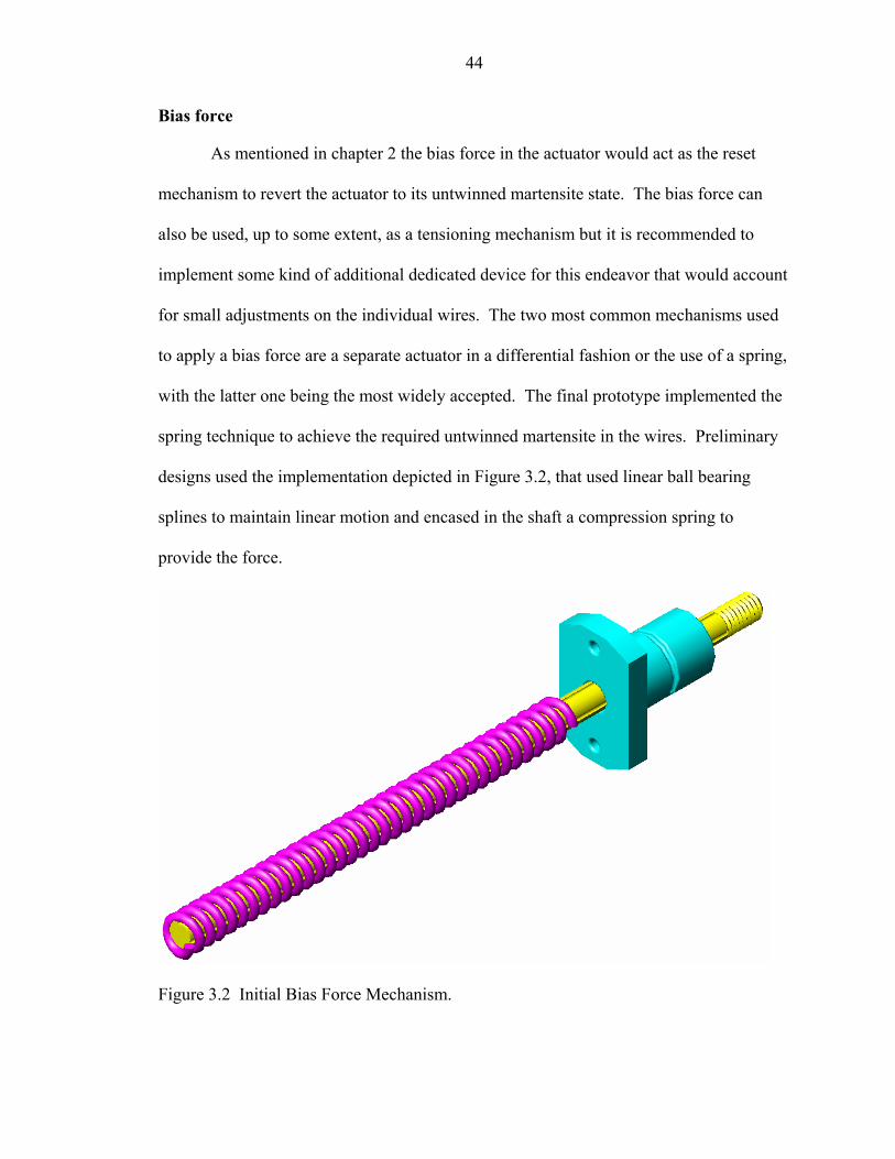
Bias force
As mentioned in chapter 2 the bias force in the actuator would act as the reset
mechanism to revert the actuator to its untwinned martensite state. The bias force can
also be used, up to some extent, as a tensioning mechanism but it is recommended to
41
implement some kind of additional dedicated device for this endeavor that would account
for small adjustments on the individual wires. The two most common mechanisms used
to apply a bias force are a separate actuator in a differential fashion or the use of a spring,
with the latter one being the most widely accepted. The final prototype implemented the
spring technique to achieve the required untwinned martensite in the wires. Preliminary
designs used the implementation depicted in Figure 3.2, that used linear ball bearing
splines to maintain linear motion and encased in the shaft a compression spring to
provide the force.
Figure 3.2. Initial Bias Force Mechanism.
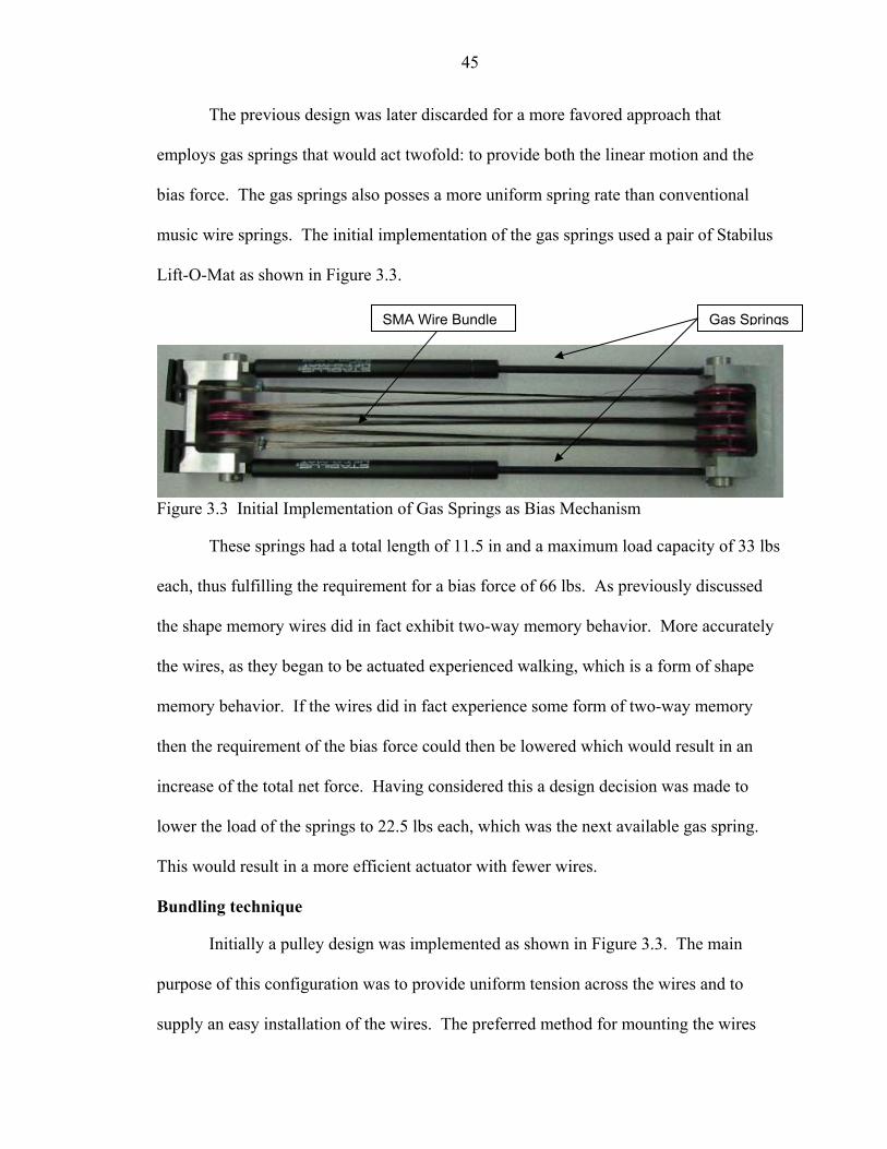
The previous design was later discarded for a more favored approach that
employs gas springs that would act twofold: to provide both the linear motion and the
bias force. The gas springs also posses a more uniform spring rate than conventional
music wire springs. The initial implementation of the gas springs used a pair of Stabilus
Lift-O-Mat as shown in Figure 3.3.
42
Figure 3.3. Initial Implementation of Gas Springs as Bias Mechanism
These springs had a total length of 11.5 in and a maximum load capacity of 33 lbs
each, thus fulfilling the requirement for a bias force of 66 lbs. As previously discussed
the shape memory wires did in fact exhibit two-way memory behavior. More accurately
the wires, as they began to be actuated experienced walking, which is a form of shape
memory behavior. If the wires did in fact experience some form of two-way memory
then the requirement of the bias force could then be lowered which would result in an
increase of the total net force. Having considered this a design decision was made to
lower the load of the springs to 22.5 lbs each, which was the next available gas spring.
This would result in a more efficient actuator with fewer wires.
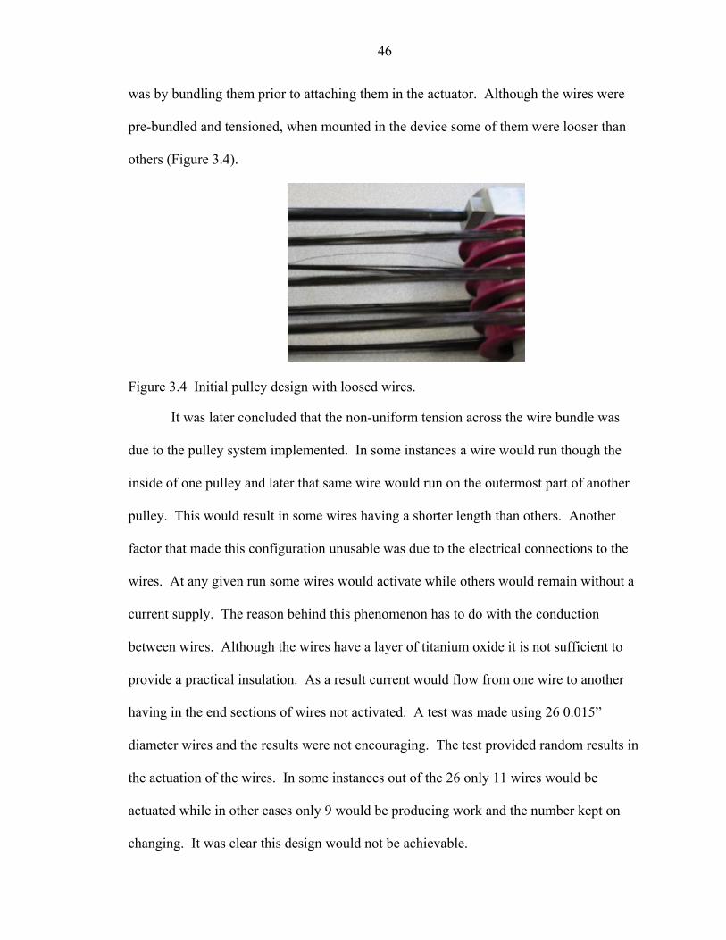
Bundling technique
Initially a pulley design was implemented as shown in Figure 3.3. The main
purpose of this configuration was to provide uniform tension across the wires and to
supply an easy installation of the wires. The preferred method for mounting the wires
was by bundling them prior to attaching them in the actuator. Although the wires were
pre-bundled and tensioned, when mounted in the device some of them were looser than
others (Figure 3.4). It was later concluded that the non-uniform tension across the wire
bundle was due to the pulley system implemented. In some instances a wire would run
though the inside of one pulley and later that same wire would run on the outermost part
Gas SpringsSMA Wire Bundle
43
of another pulley. This would result in some wires having a shorter length than others.
Another factor that made this configuration unusable was due to the electrical
connections to the wires. At any given run some wires would activate while others would
remain without a current supply. The reason behind this phenomenon has to do with the
conduction between wires. Although the wires have a layer of titanium oxide it is not
sufficient to provide a practical insulation. As a result current would flow from one wire
to another having in the end sections of wires not activated. A test was made using 26
0.015” diameter wires and the results were not encouraging. The test provided random
results in the actuation of the wires. In some instances out of the 26 only 11 wires would
be actuated while in other cases only 9 would be producing work and the number kept on
changing. It was clear this design would not be achievable.
Figure 3.4. Initial Pulley design with loosed wires.
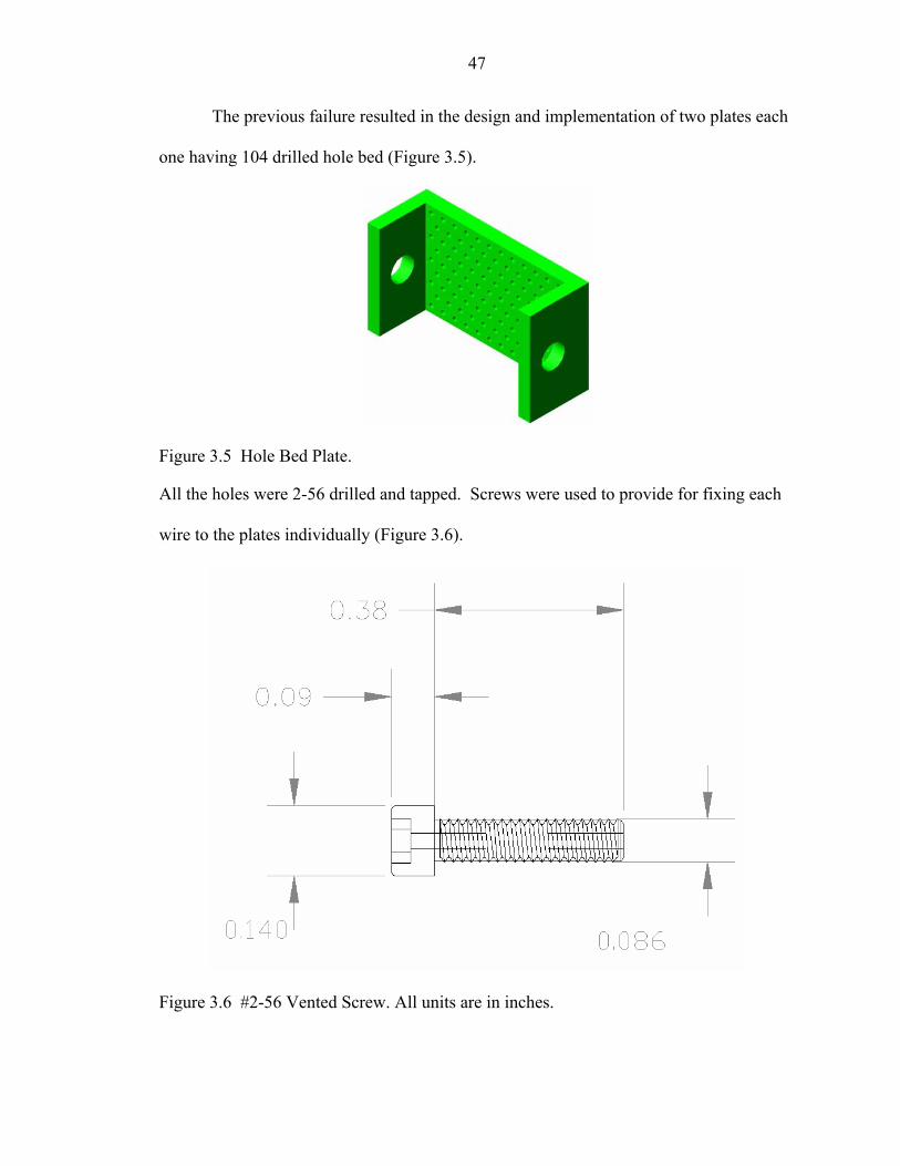
The previous failure resulted in the design and implementation of two plates each one
having 104 drilled hole bed (Figure 3.5). All the holes were 2-56 drilled and tapped.
Screws were used to provide for fixing each wire to the plates individually (Figure 3.6).
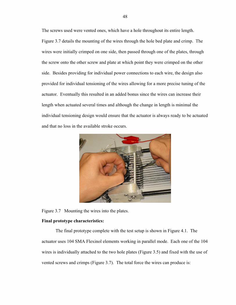
The screws used were vented ones, which have a hole throughout its entire length.
Figure 3.7 details the mounting of the wires through the hole bed plate and crimp.
The wires were initially crimped on one side, then passed through one of the plates,
44
Figure 3.5. Hole Bed Plate.
Figure 3.6. #2-56 Vented Screw. All units are in inches.
through the screw onto the other screw and plate at which point they were crimped on the
other side. Besides providing for individual power connections to each wire, the design
also provided for individual tensioning of the wires allowing for a more precise tuning of
the actuator. Eventually this resulted in an added bonus since the wires can increase their
length when actuated several times and although the change in length is minimal the
individual tensioning design would ensure that the actuator is always ready to be actuated
and that no loss in the available stroke occurs.
45
Figure 3.7. Mounting the wires into the plates.
Final prototype characteristics:
The final prototype complete with the test setup is shown in Figure 4.1. The
actuator uses 104 SMA Flexinol elements working in parallel mode. Each one of the 104
wires is individually attached to the two hole plates (Figure 3.5) and fixed with the use of
vented screws and crimps (Figure 3.7). The total force the wires can produce is:
lbslbsFNF WIREWIRESTOT ⋅=⋅⋅=⋅= 27.1353.1104 3.6
Two Stabilus Lift-O-Mat nitrogen gas springs were implemented as the bias loading
mechanism with a total length of 20 inches and a maximum pull force of 22.5 lbs each
having a total bias load of 45 lbs. The total gravitational load that the actuator will be
moving as part of the actuator itself is comprised of the sum of the weights for the bottom
C-Bracket, two blade ends, 104 #2-56 screws, and the two body rods for the gas springs.
This load comes to be approximately 3 lbs. The static force was calculated empirically to
be approximately 15 lbs. From these parameters the default load that the actuator is
subject to comes to be:
lbsFFFF BIASSGDEFAULT ⋅=++=++= 6345153 3.7
46
From this value the net load for the actuator can be obtained to be:
lbsFFF DEFAULTTOTNET ⋅=−=−= 27.726327.135 3.8
According to the manufacturers data sheet the wires in still air should contract
with a recommended current of 610 mA for a total current of 63.44 A. The contraction
time should be less than one second and the cooling or off time for relaxation should be
at about 3.5 seconds this would give a total actuation cycle time of 4.5 seconds and a
cycle rate of about 13 cycles per minute. The cycle rate can be increased by utilizing
some form of active cooling on the wires like forced air and the effects of active cooling
will be discussed in the next chapter.
47
CHAPTER 4 EXPERIMENTAL SETUP AND RESULTS
Test Platform
Hardware
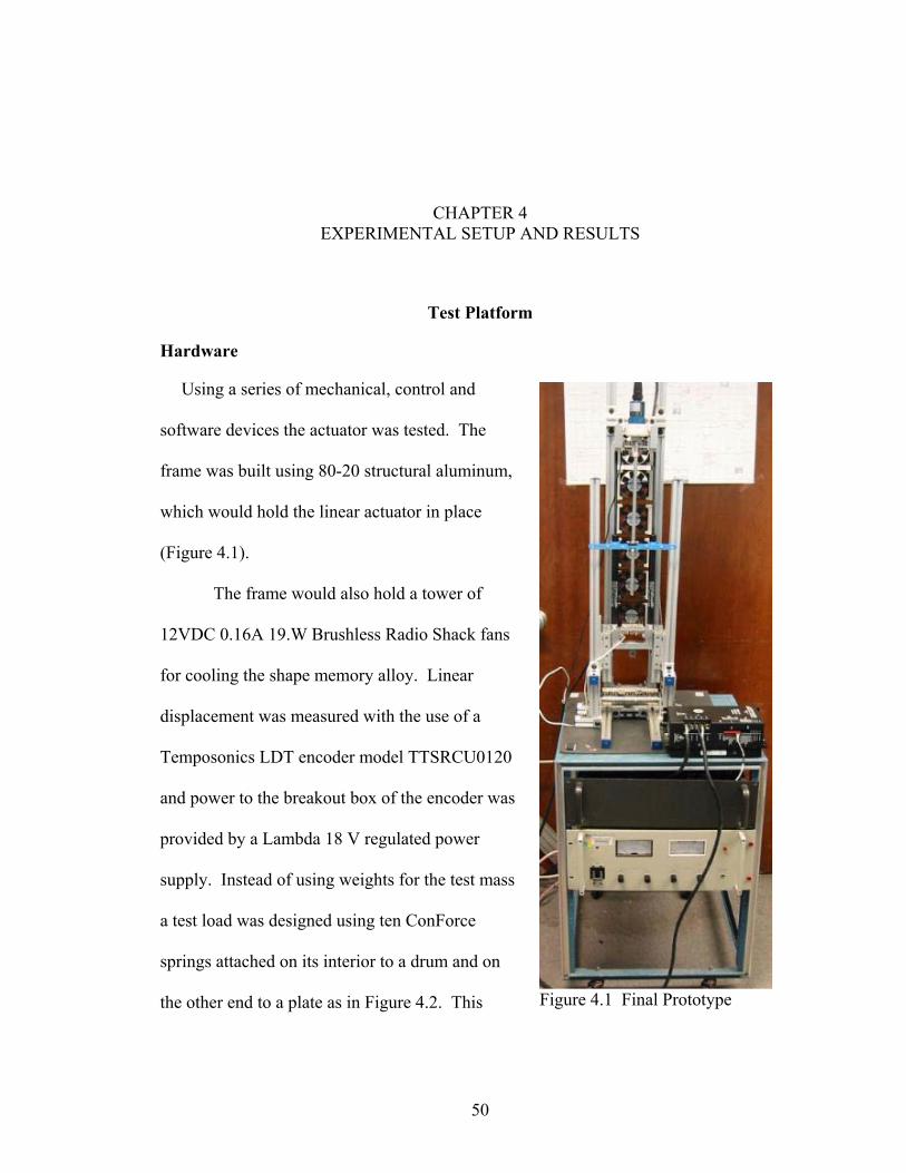
Using a series of mechanical, control and
software devices the actuator was tested. The
frame was built using 80-20 structural aluminum,
which would hold the linear actuator in place
(Figure 4.1).
The frame would also hold a tower of
12VDC 0.16A 19.W Brushless Radio Shack fans
for cooling the shape memory alloy. Linear
displacement was measured with the use of a
Temposonics LDT encoder model TTSRCU0120
and power to the breakout box of the encoder was
provided by a Lambda 18 V regulated power
supply. Instead of using weights for the test mass
a test load was designed using ten ConForce
springs attached on its interior to a drum and on
the other end to a plate as in Figure 4.2. This
Figure 4.1: Final Prototype
48
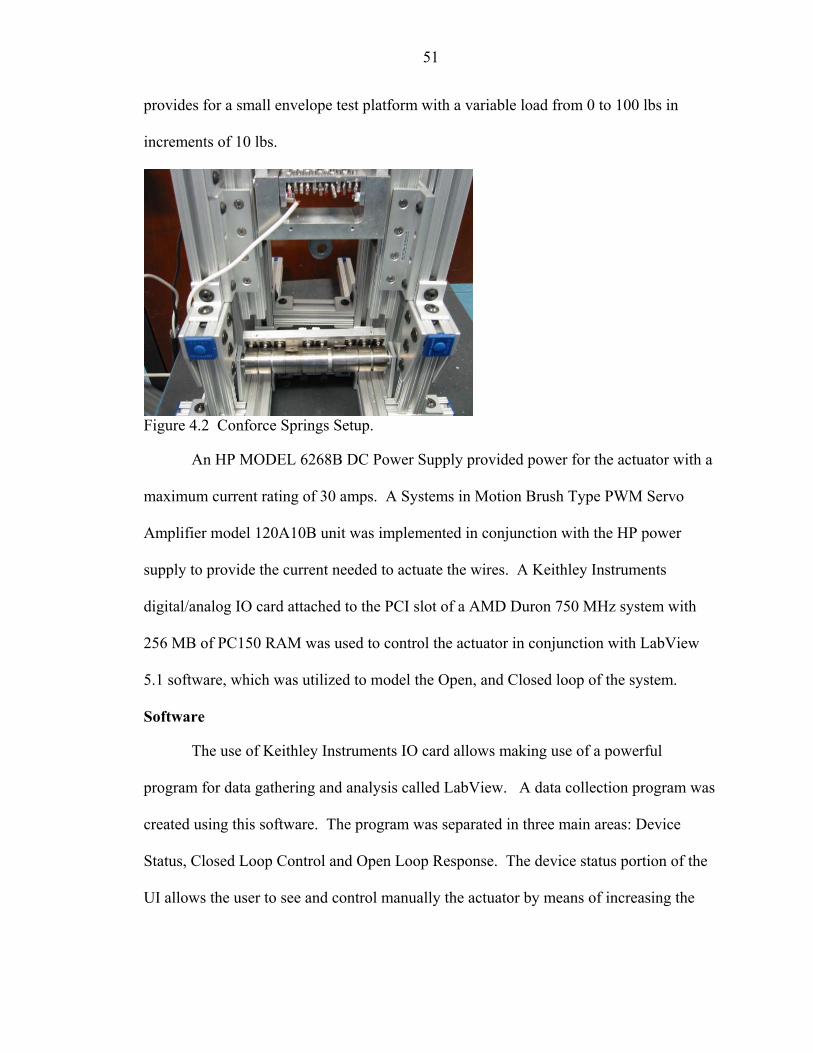
provides for a small envelope test platform with a variable load from 0 to 100 lbs in
increments of 10 lbs.
Figure 4.2: Conforce Springs Setup.
An HP MODEL 6268B DC Power Supply provided power for the actuator with a
maximum current rating of 30 amps. A Systems in Motion Brush Type PWM Servo
Amplifier model 120A10B unit was implemented in conjunction with the HP power
supply to provide the current needed to actuate the wires. A Keithley Instruments
digital/analog IO card attached to the PCI slot of a AMD Duron 750 MHz system with
256 MB of PC150 RAM was used to control the actuator in conjunction with LabView
5.1 software, which was utilized to model the Open, and Closed loop of the system.
Software
The use of Keithley Instruments IO card allows making use of a powerful
program for data gathering and analysis called LabView. A data collection program was
created using this software. The program was separated in three main areas: Device
Status, Closed Loop Control and Open Loop Response. The device status portion of the
UI allows the user to see and control manually the actuator by means of increasing the
49
reference voltage, turn on and off the cooling fans, see the current stroke as well as the
filtered and unfiltered LDT signal and turn on or off the filtering of such signal.
The open loop transient response of the actuator allows the user to record the step
response of the actuator. The user can also determine a delay time for recording, and off
time until the recording to the data file stops to measure the cooling time of the actuator
after the initial activation.
The open loop steady state response of the actuator recorded the response of the
actuator to a given input, which is being incremented when no appreciable difference in
stroke is observed. The run starts at Vref of 0V until 5V and can be incremented by a
number, which can be set by the user. The user can also set the stroke threshold.
Finally the closed loop portion of the program implements a PID controller. In
this segment of the program the user can set the PID constants namely: Kp, Ki and Kd, the
loop’s delay time and record to a file. The data is displayed visually in three charts and
can be also recorded onto a file. The User Interface of the program is displayed in Figure
4.3.
The Tests
The open and closed loop response of the actuator under still air conditions was
implemented for 104 0.008” Flexinol LT parallel configuration of wires.
Open Loop Response
Two types of open loop responses were taken: transient and steady state. The
transient open loop response acquired data for a given step input and recorded time and
stroke. The steady state response was time independent while reference voltage and
stroke was recorded.
50
Figure 4.3. LabView Virtual Instruments for the SMA Actuator.
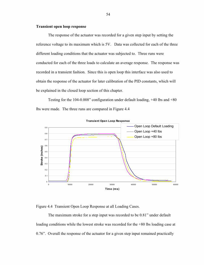
Transient open loop response
The response of the actuator was recorded for a given step input by setting the
reference voltage to its maximum which is 5V. Data was collected for each of the three
different loading conditions that the actuator was subjected to. Three runs were
conducted for each of the three loads to calculate an average response. The response was
recorded in a transient fashion. Since this is open loop this interface was also used to
51
obtain the response of the actuator for later calibration of the PID constants, which will
be explained in the closed loop section of this chapter.
Testing for the 104-0.008” configuration under default loading, +40 lbs and +80
lbs were made. The three runs are compared in Figure 4.4
Transient Open Loop Response
0
0.1
0.2
0.3
0.4
0.5
0.6
0.7
0.8
0.9
0 10000 20000 30000 40000 50000 60000
Time (ms)
Stro
ke (i
nche
s)
Open Loop Default LoadingOpen Loop +40 lbsOpen Loop +80 lbs
Figure 4.4. Transient Open Loop Response at all Loading Cases.
The maximum stroke for a step input was recorded to be 0.81” under default
loading conditions while the lowest stroke was recorded for the +80 lbs loading case at
0.76”. Overall the response of the actuator for a given step input remained practically
unchanged regardless of the load that the actuator has to pull. This will prove to be
important latter on when we discuss the calibration for closed loop control and the effects
of proportional control on the actuator.
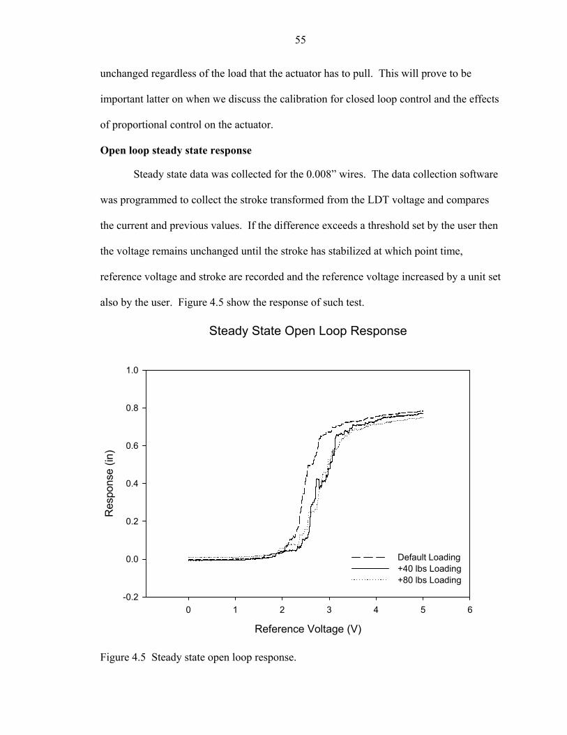
Open loop steady state response
Steady state data was collected for the 0.008” wires. The data collection software
was programmed to collect the stroke transformed from the LDT voltage and compares
52
the current and previous values. If the difference exceeds a threshold set by the user then
the voltage remains unchanged until the stroke has stabilized at which point time,
reference voltage and stroke are recorded and the reference voltage increased by a unit set
also by the user. Figure 4.5 show the response of such test.
Steady State Open Loop Response
Reference Voltage (V)
0 1 2 3 4 5 6
Res
pons
e (in
)
-0.2
0.0
0.2
0.4
0.6
0.8
1.0
Default Loading+40 lbs Loading+80 lbs Loading
Figure 4.5. Steady state open loop response.
Closed Loop Response
Closed loop response was taken for different comparison standpoints. The first
set of collected data was taken to illustrate performance of Nichols calibrated PID, PI and
P controllers. Secondary data was collected in order to compare the Nichols calibrated
PID to an optimized PID controller.
53
Overall closed loop response
Closed loop control was implemented for a PID, PI and P controllers. The
controller is software based with the stroke as the input and the reference voltage as the
output. The PID constants were obtained by using the Nichols tuning method [18]. For
the calibration open loop response was plotted as shown in Figures 4.6 through 4.8 for
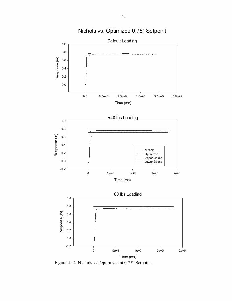
Figure 4.14: Nichols vs. Optimized at 0.75” Setpoint.
69
CHAPTER 5 CONCLUSIONS
SMA Correlations
Suffice to say that SMA related design is not an easy endeavor. Several aspects
must be considered before the final prototype takes place. One of the major obstacles to
overcome are the intertwined properties of shape memory alloys. Most of the physical,
electrical and mechanical aspects of shape memory depend on each other and at some
point design decisions must be make to reduce the number of variables. In reality a trade
back is always made. Some of these correlations are discussed next.
Force vs. Cycle Times vs. Power:
As discussed in chapter three of this work the actuation force that a shape memory
element is capable of is a function of its cross-sectional area. For a straight wire this
means a circular cross sectional area. The actuation cycle of a shape memory element is
a function of the heating and cooling times, which is a function of the heat transfer
phenomena inside the SMA which in turn has one of its parameters the cross sectional
area of the element. Without getting into specifics we know that the higher the cross
sectional area of an element the longer it will take to cool down and this will lead to a
higher actuation cycle. Based on this we know that the force of the element is directly
proportional to the time it takes the actuator to complete one full cycle. If the force
required by the SMA element is large then expect to see a slower actuator.
This drawback can be addressed by the implementation of a parallel configuration
of shape memory elements, such as the one implemented in this work. The parallel array
70
of wires can provide a higher force while maintaining a fast enough response. This
however, posses another factor to consider: power. Large cross sectional area shape
memory alloy elements are typically more efficient than lower ones, thus a trade back is
presented to the designer: which design factor is more important? If the designer is more
interested solely in force and a simplified design then a large element or a small bundle of
large elements can be considered at the expense of a slower response but with more
efficient wires. However if the most important factor to consider is the response time of
the actuator then a bundle of wires in parallel configuration to provide for the force at the
expense of more power needed to drive the device. Since shape memory alloys are
inherently inefficient it is recommended that the designer explore how much can be
gained by sacrificing the actuation times.
Stroke vs. Durability vs. Envelope Volume
As previously stated in Chapter 3 the stroke of a shape memory element is a
function of the strain the actuator is subject to. The most typical maximum strain that a
SMA can exert is in the vicinity of 8%. However, this value if implemented will lead to
less than 100 cycles after which the performance of the element will start to degrade.
The lifetime cycles can be greatly improved if the working strain is to be reduced.
Previous work has concluded that for Nitinol a strain of 5% will yield hundreds of
thousands of cycles, and the cost of a higher lifetime is a reduced actuation stroke.
Another factor that ties into this equation is the overall length of the shape memory
element, which is also a function of the stroke. The length is a factor of the envelope
volume where the actuator resides. The designer must then consider which one of these
parameters is more important in its design and a trade back will be made.
71
Advantages and Drawbacks
As of today there are few advantages for implementing a shape memory driven
actuator, especially for large-scale applications. The most attractive features reside in a
compact design, low weight and minimal sound levels. Design wise their implementation
at large scale is a difficult process to say the least. Power consumption is extremely high
when compared to technologies that can provide the same level of functionality.
However, they do offer a viable alternative to hydraulics, which is the method of choice
when handling large loads. Their inherent low weight makes them ideal for portable
designs and space exploration.
Control Aspects
This work showed that a large-scale SMA actuator is possible and although far
from perfect the actuator can be controlled within reason. The following discusses the
conclusions that were derived from testing.
1. Open loop response was repeatable and precise.
2. The output from the open loop produced a response from which Nichols tuning method can be implemented for latter use in the closed loop.
3. The steady state open loop response produced the same trend as a SMA stress strain chart.
4. Open loop case serves as an ideal implementation when only one setpoint is desired or an on/off application.
5. Time response for the open loop was around 4-5 seconds for all loading conditions.
6. A proportional controller alone cannot be used to control a shape memory based actuator. Proportional control only achieves acceptable response under the 0.75” setpoint, slightly less than the maximum stroke defined for the setup.
7. PI and PID control schemes yielded similar responses, with the PID solution having better overall responses. This indicates that the system does in fact benefit from the damping effect of the derivative controller.
72
8. Optimization for a PID controller is achievable and in the implemented optimized case the maximum performance obtained varied from a Nichols tuned PID by as much as 1300%.
Viability
A large-scale implementation of shape memory alloys although possible can
become an expensive endeavor. The cost alone of the shape memory elements indicates
that the system will be expensive but it also depends on the number of elements being
used. Custom design of shape memory elements is far more expensive than pre made
commercial ones. Case in point a single strip of Ni-Ti custom made would cost around
2000 dollars. If cost is an important factor then the commercial available forms and sizes
should be implemented and the design adjusted to accommodate to this element.
73
CHAPTER 6 FUTURE WORK
Although some headway was made for future work in this area the
implementation of SMA for large-scale control is still far from reality. The major benefit
a future researcher in this area can expect from this work comes in the form of its
extensive but practical literature review as well as pointing out possible design strategies
while avoiding some of the most time consuming pitfalls.
In terms of a practical and easy to implement actuator the design of a small stroke
actuator with a large actuation force would be a possibility while reciprocating some of
the force to an increased motion. Work has been done on this area by Gorbet [14] but the
force of his actuator has been limited.
Another possible and practical design to achieve high force and stroke can be
obtained by implementing a rotational shape memory alloy driven rotational actuator
coupled with a linear bearing spline to achieve the desired stroke. These design strategies
call for the SMA units to be actuated as an on/off device thus avoiding the complex
control at the material level.
Then there is always the most common implementation of shape memory devices
in the form of micro actuators, an area where these materials have already proven their
worth.
76
BIOGRAPHICAL SKETCH
José R. Santiago was born on December 16, 1973, in the town of Ponce, Puerto Rico.
After graduating from high school he attended the University of Puerto Rico Mayagüez
Campus, where he obtained a Bachelor of Science in mechanical engineering on 1997. In
1998 he enrolled in the graduate program of the University of Florida to pursue a
master’s degree in mechanical engineering. His focus while in this program has been
11. T. Waram, “Design Principles for Ni-Ti Actuators,” Engineering Aspects of Shape Memory Alloys, Butterworth-Heinemann Publishers, London, 1990, pp. 234-244.
12. R.C. Juvinall, and K.M. Marshek, 2nd Edition, Fundamentals of Machine Component
Design, John Wiley and Sons, Inc., NY, 1991, p.427-452. 13. Y. Nakano, M. Fujie, and Y. Hosada, “Hitachi’s Robot Hand”, Robotics Age, vol. 6,
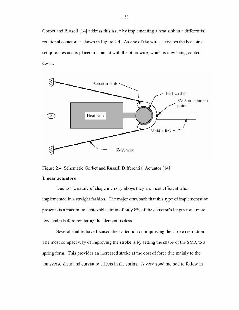
no. 7, July 1984, pp. 18-20. 14. R.B. Gorbet, and R.A. Russell, “A novel differential shape memory alloy actuator for
position control”, Robotica, vol. 13, Cambridge University Press, Cambridge, UK, 1995, pp. 423-430.
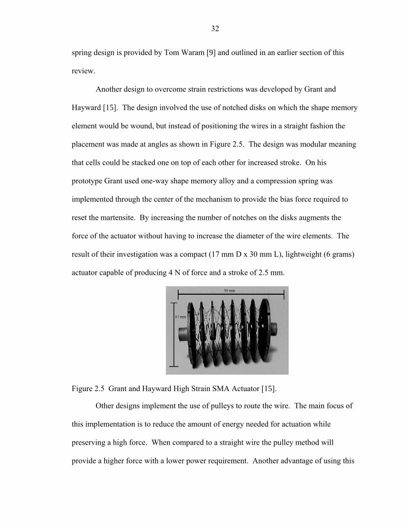
15. D Grant, V. Hayward, “Design of Shape Memory Alloy Actuator with High Strain
and Variable Structure Control,” Proceedings of 1995 IEEE International Conference on Robotics and Automation, Nagoya, Japan, vol. 3, 1995, pp. 2305-2310.
16. A.B. Soares, H.M. Brash, and D. Gow, “The Application of SMA in the Design of
Prosthetic Devices,” Preceedings of the 2nd International Conference on Shape Memory and Superelastic Technologies (SMST-97), 2-6 March 1997, Asilomar Conference Center, Pacific Grove, California, USA, SMST, Santa Clara, CA, 1997, p. 257-262.
17. M. Mosley, and C. Mavroidis, “Design and Dynamics of A Shape Memory Alloy
Wire Bundle Actuator,” Proceedings of the 2000 ASME Mechanisms and Robotics Conference, Baltimore MD, September 10-13, 2000.
18. John Van de Vegte, 3rd Edition, Feedback Control Systems, Prentice Hall, NJ, 1994,
pp. 146-147
79
BIOGRAPHICAL SKETCH
José R. Santiago was born on December 16, 1973, in the town of Ponce, Puerto Rico.
After graduating from high school he attended the University of Puerto Rico Mayagüez
Campus, where he obtained a Bachelor of Science in mechanical engineering on 1997. In
1998 he enrolled in the graduate program of the University of Florida to pursue a
master’s degree in mechanical engineering. His focus while in this program has been