Large-scale cluster management at Google with Borg · Large-scale cluster management at Google with...

Large-scale cluster management at Google

with Borg

Abhishek Verma, Luis Pedrosa, Madhukar Korupolu, David Oppenheimer, Eric Tune, John Wilkes

Google Inc.

Slides heavily derived from John Wilkes’s presentation at EuroSys, this year

Borg at Google• Cluster management system at Google that

achieves high utilization by:

• Admission control

• Efficient task-packing

• Over-commitment

• Machine sharing

The User Perspective• Users: Google developers and system administrators mainly

• The workload: Production and batch, mainly

• Cells

• Jobs and tasks

• Allocs and Alloc sets

• Priority, quota and admission control

• Naming and monitoring

The User Perspective

• job hello_world = { runtime = { cell = “ic” } //what cell should run it in? binary = ‘../hello_world_webserver’ //what program to run? args = { port = ‘%port%’ } requirements = { RAM = 100M disk = 100M CPU = 0.1 } replicas = 10000 }

The User Perspective

Elapsed Time (minutes)

Running tasks

0

2500

5000

7500

10000

0:03:000:02:30

Main Benefits

• Provides scalability to run workloads across thousands of machines

• Abstracts away the details of resource management and fault handling from users

• Operates with high reliability and availability

High-level Architecture

Large-scale cluster management at Google with BorgAbhishek Verma† Luis Pedrosa‡ Madhukar Korupolu

David Oppenheimer Eric Tune John WilkesGoogle Inc.

AbstractGoogle’s Borg system is a cluster manager that runs hun-dreds of thousands of jobs, from many thousands of differ-ent applications, across a number of clusters each with up totens of thousands of machines.

It achieves high utilization by combining admission con-trol, efficient task-packing, over-commitment, and machinesharing with process-level performance isolation. It supportshigh-availability applications with runtime features that min-imize fault-recovery time, and scheduling policies that re-duce the probability of correlated failures. Borg simplifieslife for its users by offering a declarative job specificationlanguage, name service integration, real-time job monitor-ing, and tools to analyze and simulate system behavior.

We present a summary of the Borg system architectureand features, important design decisions, a quantitative anal-ysis of some of its policy decisions, and a qualitative ex-amination of lessons learned from a decade of operationalexperience with it.

1. IntroductionThe cluster management system we internally call Borg ad-mits, schedules, starts, restarts, and monitors the full rangeof applications that Google runs. This paper explains how.

Borg provides three main benefits: it (1) hides the detailsof resource management and failure handling so its users canfocus on application development instead; (2) operates withvery high reliability and availability, and supports applica-tions that do the same; and (3) lets us run workloads acrosstens of thousands of machines effectively. Borg is not thefirst system to address these issues, but it’s one of the few op-erating at this scale, with this degree of resiliency and com-pleteness. This paper is organized around these topics, con-

† Work done while author was at Google.‡ Currently at University of Southern California.

Permission to make digital or hard copies of part or all of this work for personal orclassroom use is granted without fee provided that copies are not made or distributedfor profit or commercial advantage and that copies bear this notice and the full citationon the first page. Copyrights for third-party components of this work must be honored.For all other uses, contact the owner/author(s).EuroSys’15, April 21–24, 2015, Bordeaux, France.Copyright is held by the owner/author(s).ACM 978-1-4503-3238-5/15/04.http://dx.doi.org/10.1145/2741948.2741964

web browsers

BorgMaster

link shard

UI shardBorgMaster

link shard

UI shardBorgMaster

link shard

UI shardBorgMaster

link shard

UI shard

Cell

Scheduler

borgcfg command-line tools web browsers

scheduler

Borglet Borglet Borglet Borglet

BorgMaster

link shard

read/UI shard

config file

persistent store (Paxos)

Figure 1: The high-level architecture of Borg. Only a tiny fractionof the thousands of worker nodes are shown.

cluding with a set of qualitative observations we have madefrom operating Borg in production for more than a decade.

2. The user perspectiveBorg’s users are Google developers and system administra-tors (site reliability engineers or SREs) that run Google’sapplications and services. Users submit their work to Borgin the form of jobs, each of which consists of one or moretasks that all run the same program (binary). Each job runsin one Borg cell, a set of machines that are managed as aunit. The remainder of this section describes the main fea-tures exposed in the user view of Borg.

2.1 The workloadBorg cells run a heterogenous workload with two main parts.The first is long-running services that should “never” godown, and handle short-lived latency-sensitive requests (afew µs to a few hundred ms). Such services are used forend-user-facing products such as Gmail, Google Docs, andweb search, and for internal infrastructure services (e.g.,BigTable). The second is batch jobs that take from a fewseconds to a few days to complete; these are much less sen-sitive to short-term performance fluctuations. The workloadmix varies across cells, which run different mixes of applica-tions depending on their major tenants (e.g., some cells arequite batch-intensive), and also varies over time: batch jobs

Elapsed Time (minutes)

Running tasks

0

2500

5000

7500

10000

0:03:000:02:30

9933

Failures

prodnon-prod

0 1 2 3 4 5 6 7 8Evictions per task-week

machine shutdownother

out of resourcesmachine failurepreemption

Figure 3: Task-eviction rates and causes for production and non-production workloads. Data from August 1st 2013.

these keep the 99%ile response time of the UI below 1 sand the 95%ile of the Borglet polling interval below 10 s.

Several things make the Borg scheduler more scalable:Score caching: Evaluating feasibility and scoring a ma-

chine is expensive, so Borg caches the scores until the prop-erties of the machine or task change – e.g., a task on the ma-chine terminates, an attribute is altered, or a task’s require-ments change. Ignoring small changes in resource quantitiesreduces cache invalidations.

Equivalence classes: Tasks in a Borg job usually haveidentical requirements and constraints, so rather than deter-mining feasibility for every pending task on every machine,and scoring all the feasible machines, Borg only does fea-sibility and scoring for one task per equivalence class – agroup of tasks with identical requirements.

Relaxed randomization: It is wasteful to calculate fea-sibility and scores for all the machines in a large cell, so thescheduler examines machines in a random order until it hasfound “enough” feasible machines to score, and then selectsthe best within that set. This reduces the amount of scoringand cache invalidations needed when tasks enter and leavethe system, and speeds up assignment of tasks to machines.Relaxed randomization is somewhat akin to the batch sam-pling of Sparrow [65] while also handling priorities, preemp-tions, heterogeneity and the costs of package installation.

In our experiments (§5), scheduling a cell’s entire work-load from scratch typically took a few hundred seconds, butdid not finish after more than 3 days when the above tech-niques were disabled. Normally, though, an online schedul-ing pass over the pending queue completes in less than halfa second.

4. AvailabilityFailures are the norm in large scale systems [10, 11, 22].Figure 3 provides a breakdown of task eviction causes in15 sample cells. Applications that run on Borg are expectedto handle such events, using techniques such as replication,storing persistent state in a distributed file system, and (ifappropriate) taking occasional checkpoints. Even so, we tryto mitigate the impact of these events. For example, Borg:• automatically reschedules evicted tasks, on a new ma-

chine if necessary;• reduces correlated failures by spreading tasks of a job

across failure domains such as machines, racks, andpower domains;

• limits the allowed rate of task disruptions and the numberof tasks from a job that can be simultaneously down

65 70 75 80 85 90 95 1000

20

40

60

80

100

Compacted size [%]

Pe

rce

nta

ge

of

cells

Figure 4: The effects of compaction. A CDF of the percentage oforiginal cell size achieved after compaction, across 15 cells.

during maintenance activities such as OS or machineupgrades;

• uses declarative desired-state representations and idem-potent mutating operations, so that a failed client canharmlessly resubmit any forgotten requests;

• rate-limits finding new places for tasks from machinesthat become unreachable, because it cannot distinguishbetween large-scale machine failure and a network parti-tion;

• avoids repeating task::machine pairings that cause task ormachine crashes; and

• recovers critical intermediate data written to local disk byrepeatedly re-running a logsaver task (§2.4), even if thealloc it was attached to is terminated or moved to anothermachine. Users can set how long the system keeps trying;a few days is common.

A key design feature in Borg is that already-running taskscontinue to run even if the Borgmaster or a task’s Borgletgoes down. But keeping the master up is still importantbecause when it is down new jobs cannot be submittedor existing ones updated, and tasks from failed machinescannot be rescheduled.

Borgmaster uses a combination of techniques that enableit to achieve 99.99% availability in practice: replication formachine failures; admission control to avoid overload; anddeploying instances using simple, low-level tools to mini-mize external dependencies. Each cell is independent of theothers to minimize the chance of correlated operator errorsand failure propagation. These goals, not scalability limita-tions, are the primary argument against larger cells.

5. UtilizationOne of Borg’s primary goals is to make efficient use ofGoogle’s fleet of machines, which represents a significantfinancial investment: increasing utilization by a few percent-age points can save millions of dollars. This section dis-cusses and evaluates some of the policies and techniques thatBorg uses to do so.

Efficiency: Is Borg’s policy the best for utilizing clusters?

• Advanced Bin-Packing algorithms:

• Avoid stranding of resources

• Evaluation metric: Cell-compaction

• Find the smallest cell that we can pack the workload into…

• Remove machines randomly from a cell to maintain cell heterogeneity

• Evaluated various policies to understand the cost, in terms of extra machines needed for packing the same workload

Should we share cluster?• …between production and non-production

workloads?

A B C D E0

50

100

150

200

Cell

Pe

rce

nta

ge

of

cell

prod non-prod baseline unused

(a) The left column for each cell shows the original size and thecombined workload; the right one shows the segregated case.

-10 0 10 20 30 40 50 600

20

40

60

80

100

Overhead from segregation [%]

Perc

enta

ge o

f ce

lls

(b) CDF of additional machines that would be needed if wesegregated the workload of 15 representative cells.

Figure 5: Segregating prod and non-prod work into different cells would need more machines. Both graphs show how many extra machineswould be needed if the prod and non-prod workloads were sent to separate cells, expressed as a percentage of the minimum number ofmachines required to run the workload in a single cell. In this, and subsequent CDF plots, the value shown for each cell is derived from the90%ile of the different cell sizes our experiment trials produced; the error bars show the complete range of values from the trials.

5.1 Evaluation methodologyOur jobs have placement constraints and need to handle rareworkload spikes, our machines are heterogenous, and werun batch jobs in resources reclaimed from service jobs. So,to evaluate our policy choices we needed a more sophisti-cated metric than “average utilization”. After much exper-imentation we picked cell compaction: given a workload,we found out how small a cell it could be fitted into byremoving machines until the workload no longer fitted, re-peatedly re-packing the workload from scratch to ensure thatwe didn’t get hung up on an unlucky configuration. Thisprovided clean termination conditions and facilitated auto-mated comparisons without the pitfalls of synthetic work-load generation and modeling [31]. A quantitative compari-son of evaluation techniques can be found in [78]: the detailsare surprisingly subtle.

It wasn’t possible to perform experiments on live produc-tion cells, but we used Fauxmaster to obtain high-fidelitysimulation results, using data from real production cellsand workloads, including all their constraints, actual lim-its, reservations, and usage data (§5.5). This data camefrom Borg checkpoints taken on Wednesday 2014-10-0114:00 PDT. (Other checkpoints produced similar results.)We picked 15 Borg cells to report on by first eliminatingspecial-purpose, test, and small (< 5000 machines) cells,and then sampled the remaining population to achieve aroughly even spread across the range of sizes.

To maintain machine heterogeneity in the compacted cellwe randomly selected machines to remove. To maintainworkload heterogeneity, we kept it all, except for server andstorage tasks tied to a particular machine (e.g., the Borglets).We changed hard constraints to soft ones for jobs larger thanhalf the original cell size, and allowed up to 0.2% tasks to gopending if they were very “picky” and could only be placedon a handful of machines; extensive experiments showedthat this produced repeatable results with low variance. If

Figure 6: Segregating users would need more machines. The totalnumber of cells and the additional machines that would be neededif users larger than the threshold shown were given their ownprivate cells, for 5 different cells.

we needed a larger cell than the original we cloned the orig-inal cell a few times before compaction; if we needed morecells, we just cloned the original.

Each experiment was repeated 11 times for each cell withdifferent random-number seeds. In the graphs, we use an er-ror bar to display the min and max of the number of ma-chines needed, and select the 90%ile value as the “result” –the mean or median would not reflect what a system admin-istrator would do if they wanted to be reasonably sure thatthe workload would fit. We believe cell compaction providesa fair, consistent way to compare scheduling policies, and ittranslates directly into a cost/benefit result: better policiesrequire fewer machines to run the same workload.

Our experiments focused on scheduling (packing) aworkload from a point in time, rather than replaying a long-term workload trace. This was partly to avoid the difficultiesof coping with open and closed queueing models [71, 79],partly because traditional time-to-completion metrics don’tapply to our environment with its long-running services,partly to provide clean signals for making comparisons,

• Segregating them would need more machines!

Why such large cells?• Should we split them into smaller cells?

2 4 6 8 10-20

0

20

40

60

80

Sub-cells

Ove

rhe

ad

[%

]

cell A

cell B

cell C

cell D

cell E

(a) Additional machines that would be needed as a function ofthe number of smaller cells for five different original cells.

-50 0 50 100 150 200 2500

20

40

60

80

100

Overhead from partitioning [%]

Pe

rce

nta

ge

of

cells

2 subcells

5 subcells

10 subcells

(b) A CDF of additional machines that would be needed todivide each of 15 different cells into 2, 5 or 10 cells.

Figure 7: Subdividing cells into smaller ones would require more machines. The additional machines (as a percentage of the single-cellcase) that would be needed if we divided these particular cells into a varying number of smaller cells.

partly because we don’t believe the results would be sig-nificantly different, and partly a practical matter: we foundourselves consuming 200 000 Borg CPU cores for our ex-periments at one point—even at Google’s scale, this is anon-trivial investment.

In production, we deliberately leave significant headroomfor workload growth, occasional “black swan” events, loadspikes, machine failures, hardware upgrades, and large-scalepartial failures (e.g., a power supply bus duct). Figure 4shows how much smaller our real-world cells would be ifwe were to apply cell compaction to them. The baselines inthe graphs that follow use these compacted sizes.

5.2 Cell sharingNearly all of our machines run both prod and non-prod tasksat the same time: 98% of the machines in shared Borg cells,83% across the entire set of machines managed by Borg. (Wehave a few dedicated cells for special uses.)

Since many other organizations run user-facing and batchjobs in separate clusters, we examined what would happen ifwe did the same. Figure 5 shows that segregating prod andnon-prod work would need 20–30% more machines in themedian cell to run our workload. That’s because prod jobsusually reserve resources to handle rare workload spikes, butdon’t use these resources most of the time. Borg reclaims theunused resources (§5.5) to run much of the non-prod work,so we need fewer machines overall.

Most Borg cells are shared by thousands of users. Figure6 shows why. For this test, we split off a user’s workloadinto a new cell if they consumed at least 10 TiB of mem-ory (or 100 TiB). Our existing policy looks good: even withthe larger threshold, we would need 2–16⇥ as many cells,and 20–150% additional machines. Once again, pooling re-sources significantly reduces costs.

But perhaps packing unrelated users and job types ontothe same machines results in CPU interference, and so wewould need more machines to compensate? To assess this,we looked at how the CPI (cycles per instruction) changed

for tasks in different environments running on the same ma-chine type with the same clock speed. Under these condi-tions, CPI values are comparable and can be used as a proxyfor performance interference, since a doubling of CPI dou-bles the runtime of a CPU-bound program. The data wasgathered from ⇠ 12000 randomly selected prod tasks overa week, counting cycles and instructions over a 5 minute in-terval using the hardware profiling infrastructure describedin [83], and weighting samples so that every second of CPUtime is counted equally. The results were not clear-cut.

(1) We found that CPI was positively correlated withtwo measurements over the same time interval: the overallCPU usage on the machine, and (largely independently) thenumber of tasks on the machine; adding a task to a machineincreases the CPI of other tasks by 0.3% (using a linearmodel fitted to the data); increasing machine CPU usage by10% increases CPI by less than 2%. But even though thecorrelations are statistically significant, they only explain 5%of the variance we saw in CPI measurements; other factorsdominate, such as inherent differences in applications andspecific interference patterns [24, 83].

(2) Comparing the CPIs we sampled from shared cells toones from a few dedicated cells with less diverse applica-tions, we saw a mean CPI of 1.58 (s = 0.35) in shared cellsand a mean of 1.53 (s = 0.32) in dedicated cells – i.e., CPUperformance is about 3% worse in shared cells.

(3) To address the concern that applications in differentcells might have different workloads, or even suffer selectionbias (maybe programs that are more sensitive to interferencehad been moved to dedicated cells), we looked at the CPI ofthe Borglet, which runs on all the machines in both types ofcell. We found it had a CPI of 1.20 (s = 0.29) in dedicatedcells and 1.43 (s = 0.45) in shared ones, suggesting thatit runs 1.19⇥ as fast in a dedicated cell as in a sharedone, although this over-weights the effect of lightly loadedmachines, slightly biasing the result in favor of dedicatedcells.

• …might end up having to partition workload across multiple sub-clusters

• would need more machines

• …might be useful to share a cell between users

Should we make cells even larger?

• Failure containment

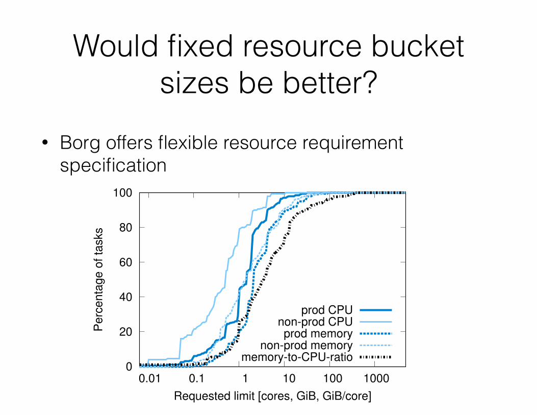
Would fixed resource bucket sizes be better?

• Borg offers flexible resource requirement specification

0

20

40

60

80

100

0.01 0.1 1 10 100 1000

Perc

enta

ge o

f ta

sks

Requested limit [cores, GiB, GiB/core]

prod CPUnon-prod CPUprod memory

non-prod memorymemory-to-CPU-ratio

Figure 8: No bucket sizes fit most of the tasks well. CDF ofrequested CPU and memory requests across our sample cells. Noone value stands out, although a few integer CPU core sizes aresomewhat more popular.

-20 0 20 40 60 80 100 1200

20

40

60

80

100

Overhead [%]

Pe

rce

nta

ge

of

cells

upper bound

lower bound

Figure 9: “Bucketing” resource requirements would need moremachines. A CDF of the additional overheads that would resultfrom rounding up CPU and memory requests to the next nearestpowers of 2 across 15 cells. The lower and upper bounds straddlethe actual values (see the text).

These experiments confirm that performance compar-isons at warehouse-scale are tricky, reinforcing the observa-tions in [51], and also suggest that sharing doesn’t drasticallyincrease the cost of running programs.

But even assuming the least-favorable of our results, shar-ing is still a win: the CPU slowdown is outweighed by thedecrease in machines required over several different parti-tioning schemes, and the sharing advantages apply to all re-sources including memory and disk, not just CPU.

5.3 Large cellsGoogle builds large cells, both to allow large computationsto be run, and to decrease resource fragmentation. We testedthe effects of the latter by partitioning the workload for a cellacross multiple smaller cells – by first randomly permutingthe jobs and then assigning them in a round-robin manneramong the partitions. Figure 7 confirms that using smallercells would require significantly more machines.

0 10 20 30 40 500

20

40

60

80

100

Overhead [%]

Pe

rce

nta

ge

of

clu

ste

rs

Figure 10: Resource reclamation is quite effective. A CDF of theadditional machines that would be needed if we disabled it for 15representative cells.

0

20

40

60

80

100

0 20 40 60 80 100 120 140

Perc

enta

ge o

f ta

sks

Ratio [%]

CPU reservation/limitmemory reservation/limit

CPU usage/limitmemory usage/limit

Figure 11: Resource estimation is successful at identifying unusedresources. The dotted lines shows CDFs of the ratio of CPU andmemory usage to the request (limit) for tasks across 15 cells. Mosttasks use much less than their limit, although a few use more CPUthan requested. The solid lines show the CDFs of the ratio of CPUand memory reservations to the limits; these are closer to 100%.The straight lines are artifacts of the resource-estimation process.

5.4 Fine-grained resource requestsBorg users request CPU in units of milli-cores, and memoryand disk space in bytes. (A core is a processor hyperthread,normalized for performance across machine types.) Figure 8shows that they take advantage of this granularity: there arefew obvious “sweet spots” in the amount of memory or CPUcores requested, and few obvious correlations between theseresources. These distributions are quite similar to the onespresented in [68], except that we see slightly larger memoryrequests at the 90%ile and above.

Offering a set of fixed-size containers or virtual machines,although common among IaaS (infrastructure-as-a-service)providers [7, 33], would not be a good match to our needs.To show this, we “bucketed” CPU core and memory resourcelimits for prod jobs and allocs (§2.4) by rounding them up tothe next nearest power of two in each resource dimension,starting at 0.5 cores for CPU and 1 GiB for RAM. Figure 9shows that doing so would require 30–50% more resourcesin the median case. The upper bound comes from allocatingan entire machine to large tasks that didn’t fit after quadru-

Bucketing resource requirements

• …would need more machines

0

20

40

60

80

100

0.01 0.1 1 10 100 1000P

erc

enta

ge o

f ta

sks





-20 0 20 40 60 80 100 1200

20

40

60

80

100

Overhead [%]

Perc

enta

ge o

f ce

lls

upper bound

lower bound





0 10 20 30 40 500

20

40

60

80

100

Overhead [%]

Perc

enta

ge

of cl

ust

ers


0

20

40

60

80

100

0 20 40 60 80 100 120 140

Perc

enta

ge o

f ta

sks

Ratio [%]






Resource Reclamation

Time

Amount of resources requested

Amount of resources

actually used

Potentially reusable resources

Effectiveness of resource reclamation

• would end up using more machines if resources aren’t reclaimed

0

20

40

60

80

100

0.01 0.1 1 10 100 1000

Pe

rce

nta

ge

of

task

s





-20 0 20 40 60 80 100 1200

20

40

60

80

100

Overhead [%]

Pe

rce

nta

ge

of

cells

upper bound

lower bound





0 10 20 30 40 500

20

40

60

80

100

Overhead [%]

Pe

rce

nta

ge

of

clu

ste

rs


0

20

40

60

80

100

0 20 40 60 80 100 120 140

Pe

rce

nta

ge

of

task

s

Ratio [%]






Users can focus on their application

Containers

• Google runs everything inside containers, even their VMs

• Containers provide:

• resource isolation

• execution isolation

Kubernetes• An open-source cluster manager derived from Borg

• Also runs on the Google Compute Cloud

• Directly derived:

• Borglet => Kubelet

• alloc => pod

• Borg containers => docker

• Declarative specifications

• Improved:

• Job => labels

• managed ports => IP per pod

• Monolithic master => micro-services

Summary

• Resiliency: A lot of attention is given to fault tolerance

• Efficiency: share resources between users, between workloads, reclaim unused resources

• Kubernetes: containers enables users to focus on their applications

Date post:	20-Mar-2019
Category:	Documents
Upload:	lamtruc
View:	217 times
Download:	0 times

Large-scale cluster management at Google with Borg · Large-scale cluster management at Google with...

Documents