Large-scale Graph Analysis Kamesh Madduri Computational Research Division Lawrence Berkeley National Laboratory [email protected] madduri.org Discovery 2015: HPC and Cloud Computing Workshop June 17, 2011
• Can process graphs with billions of vertices and edges. • Open-source:
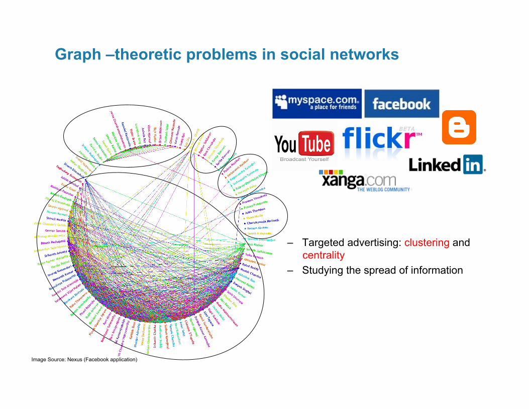
Image Source: visualcomplexity.com
snap-graph.sf.net
SNAP: Small-world Network Analysis and Partitioning
SNAP Optimizations for real-world graphs
• Preprocessing kernels (connected components, biconnected components, sparsification) significantly reduce computation time. – ex. A high number of isolated and degree-1 vertices
store BFS/Shortest Path trees from high degree vertices and reuse them
Typically 3-5X performance improvement
• Exploit small-world network properties (low graph diameter) – Load balancing in the level-synchronous parallel BFS
algorithm – SNAP data structures are optimized for unbalanced
degree distributions
• Boost Graph Library – C++, graph interface and components are generic
• NERSC Franklin system is ranked #2 on Nov 2010 list. – BFS using 500 nodes of Franklin
• Graph 500 June 2011 list submissions – NERSC Hopper, 25 GTEPS, SCALE 37,
1800 nodes – NERSC Franklin, 16 GTEPS, SCALE 36,
4000 nodes
Graph 500 “Search” Benchmark (graph500.org)
A. Buluc, K. Madduri, Proc. SC 2011
• Large-scale graph analytics: Introduction and motivating examples
• Designing parallel graph analysis algorithms and software
• Application case studies – Community Identification in social networks – RDF data analysis using compressed bitmap indexes
Talk Outline
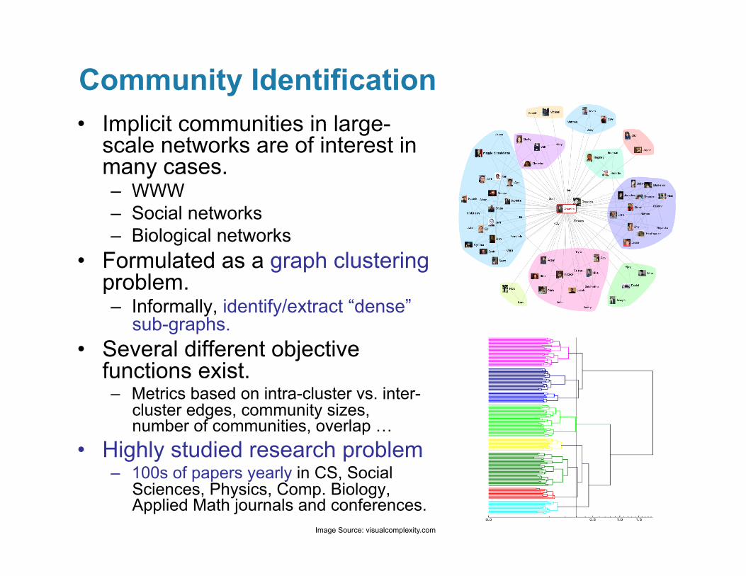
• Implicit communities in large-scale networks are of interest in many cases. – WWW – Social networks – Biological networks
• Formulated as a graph clustering problem. – Informally, identify/extract “dense”
sub-graphs. • Several different objective
functions exist. – Metrics based on intra-cluster vs. inter-
cluster edges, community sizes, number of communities, overlap …
• Highly studied research problem – 100s of papers yearly in CS, Social
Sciences, Physics, Comp. Biology, Applied Math journals and conferences.
Community Identification
Image Source: visualcomplexity.com
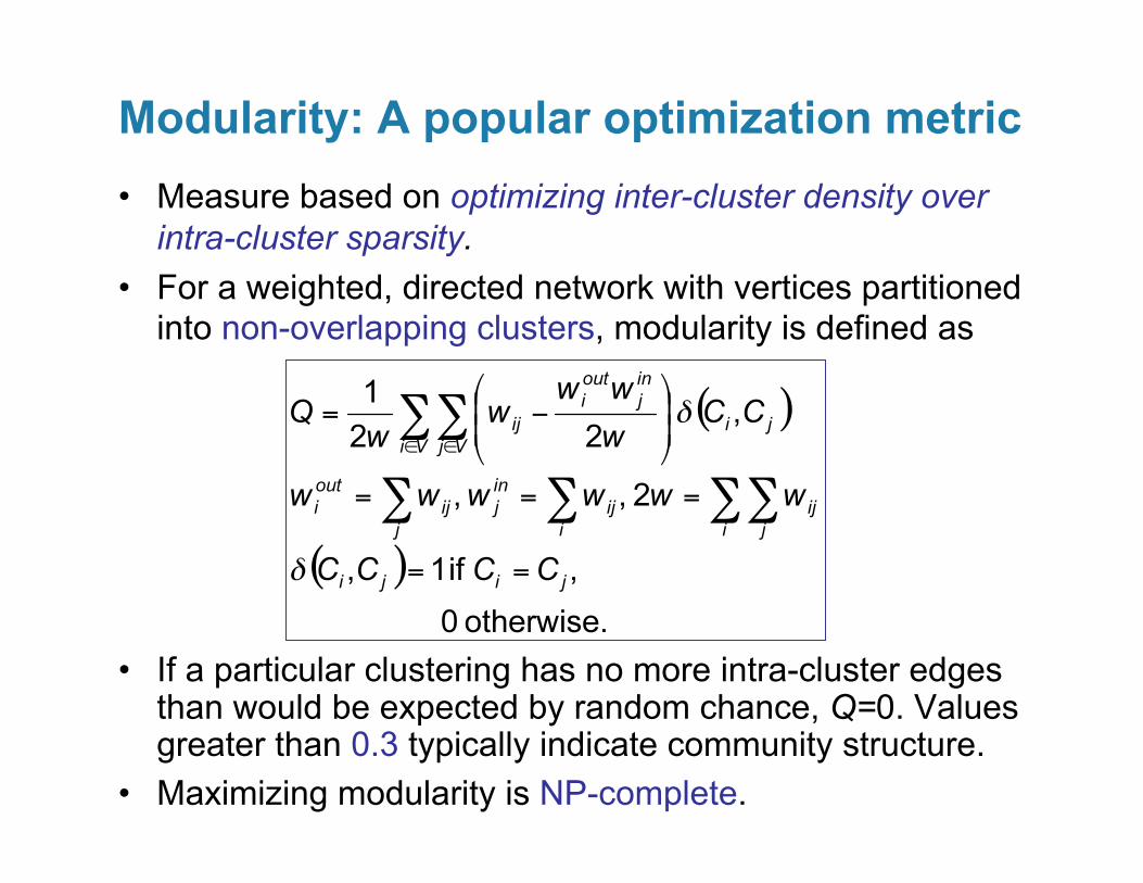
• Measure based on optimizing inter-cluster density over intra-cluster sparsity.
• For a weighted, directed network with vertices partitioned into non-overlapping clusters, modularity is defined as
• If a particular clustering has no more intra-cluster edges than would be expected by random chance, Q=0. Values greater than 0.3 typically indicate community structure.
• Maximizing modularity is NP-complete.
Modularity: A popular optimization metric
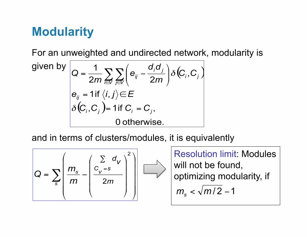
For an unweighted and undirected network, modularity is given by
and in terms of clusters/modules, it is equivalently
Modularity
Resolution limit: Modules will not be found, optimizing modularity, if
• New parallel algorithms for modularity-optimizing community identification. – Divisive: edge betweenness-based, spectral – Agglomerative – Hybrid, multi-level
• Several algorithmic optimizations for small-world networks.
• Analysis of large-scale complex networks constructed from real data.
• Note: No single “right” community detection algorithm exists. Community structure analysis should be user-driven and application-specific, combining various fast algorithms.
Our Contributions
Bader and Madduri, “SNAP”, IPDPS 2008.
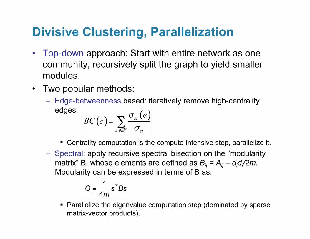
• Top-down approach: Start with entire network as one community, recursively split the graph to yield smaller modules.
• Two popular methods: – Edge-betweenness based: iteratively remove high-centrality
edges.
Centrality computation is the compute-intensive step, parallelize it. – Spectral: apply recursive spectral bisection on the “modularity
matrix” B, whose elements are defined as Bij = Aij – didj/2m. Modularity can be expressed in terms of B as:
Parallelize the eigenvalue computation step (dominated by sparse matrix-vector products).
Divisive Clustering, Parallelization
• Bottom-up approach: Start with n singleton communities, iteratively merge pairs to form larger communities. – What measure to minimize/maximize? modularity – How do we order merges? priority queue
• Run greedy agglomerative approach once graph is less than size threshold.
Hybrid approaches: Parallelization
4 6 1 1 1
Assembled a collection for algorithm performance analysis, from some of the largest publicly-available network data.
Real-world data
Name # vertices # edges Type Amazon-2003 473.30 K 3.50 M co-purchaser eu-2005 862.00 K 19.23 M www Flickr 1.86 M 22.60 M social wiki-Talk 2.40 M 5.02 M collab orkut 3.07 M 223.00 M social cit-Patents 3.77 M 16.50 M cite Livejournal 5.28 M 77.40 M social uk-2002 18.50 M 198.10 M www USA-road 23.90 M 29.00 M Transp. webbase-2001 118.14 M 1.02 B www
SNAP vs. Other Implementations (serial performance)
Webbase-2001 (n=118M, m=1.02B)
Largest network analyzed in prior papers.
SNAP 4x faster! Requires 12 GB memory vs. 30 GB for Louvain algorithm.
Amazon-2003 (n=473K, m=3.5M)
igraph: C library for network analysis. SNAP requires 0.5 GB memory vs. 12 GB+ for igraph CNM implementation!
igraph time ~ 8 hours.
Results on a Intel Xeon 5560 (“Nehalem”) system • 2 sockets x 4 cores x 2-way SMT • 12 GB DRAM, 8 MB shared L3 • 51.2 GBytes/sec peak bandwidth • 2.66 GHz proc.
SNAP Algorithms: Comparative Performance
Amazon-2003 (n=473K, m=3.5M)
• Smallest network in the test suite. • Divisive edgeBC and basic agglomerative clustering algorithm (CNM) highly compute-intensive. • CNM-RAT (comm. sizes factored in) significantly faster than CNM.
~1.5 min. <1 s.
~500 min.
Performance results on a Intel Xeon 5560 (Nehalem) system.
Communities: Sizes and Cardinality
# of communities CNM 240 Spectral 10K Hybrid 196
Amazon-2003 (n=473K, m=3.5M)
Spectral alg. fails to resolve communities beyond one level of the agglomerative clustering dendrogram!
CNM
Spectral
Communities: Modularity
• Hybrid approach performs surprisingly well. • # of communities from CNM-RAT and Hybrid roughly the same. • CNM-RAT suffers in modularity quality. • CNM did not finish (> 6hrs) for most networks.
• Goal: Avoid computing from scratch. • Consider path-based problems:
– Are there paths connecting s and t between time T1 and T2? – Does the path between s and t shorten drastically? – Is a vertex suddenly very central?
• Contribution: New space-efficient data structures, fast algorithms for dynamic network analysis.
Dynamic graph computations
Link-cut tree for answering connectivity queries. Performance results on Sun Fire T5140. 10 million vertices, 80 million edges
Construction time Query time (1 million queries)
Madduri and Bader, IPDPS’09.
• Large-scale graph analytics: Introduction and motivating examples
• Designing parallel graph analysis algorithms and software
• Application case studies – Community Identification in social networks – RDF data analysis using compressed bitmap indexes
Talk Outline
• The RDF (Resource Description Framework) data model is a popular abstraction for linked data repositories – triple form [<subject> <predicate> <object>]
– Data sets with a few billion triples quite common
• Emergence of “triple stores”, custom databases for storage and retrieval of RDF data – Jena, Virtuoso, Sesame
Semantic data analysis
• We use the compressed bitmap indexing software FastBit to index RDF data
• Search queries on RDF data can be accelerated with use of compressed bitmap indexes
• Our Contributions: – Parallel bitmap index construction (we store the sparse graphs
corresponding to each unique predicate) – New query-answering approach: pattern matching queries on
RDF data are modified to use bitmap indexes.
• Speedup insight: SPARQL queries can be expressed as fast and I/O optimal bit vector operations.
Search Query: list of all scientists born in a city in USA, who have/had a Doctoral advisor born in Chinese city.
join Index lookup
The ordering of bit vector operations determines query work performed.
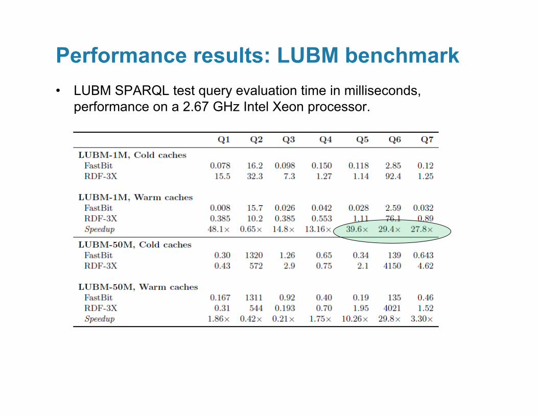
• LUBM SPARQL test query evaluation time in milliseconds, performance on a 2.67 GHz Intel Xeon processor.
Performance results: LUBM benchmark
• The SNAP (snap-graph.sf.net) framework offers novel parallel methods for social and information network analytics
– Two orders of magnitude faster than competing “serial” software approaches
• We have designed the first parallel methods for several community detection formulations
• Ongoing research projects – Semantic data analytics using compressed bitmap
indexes
– Eulerian path-based de novo genome assembly
• Future research direction: Modeling network dynamics; persistent monitoring of dynamically changing properties
Summary: Our Research Enables Complex Data-intensive Applications
BIG DATA
Analy'cs, Summariza'on, Visualiza'on
Modeling & Simula'on
• Scientific Data Management & Future Technologies research groups, LBNL
• Prof. David A. Bader, Georgia Institute of Technology • Jonathan Berry, Bruce Hendrickson (Sandia National Laboratories) • John Feo, Daniel Chavarria (Pacific Northwest National
Laboratories) • PNNL CASS-MT Center and Cray Inc. for access to their XMT
systems. • Par Lab @ UC Berkeley for access to their Millennium cluster
systems. • Research supported in part by DOE Office of Science under contract
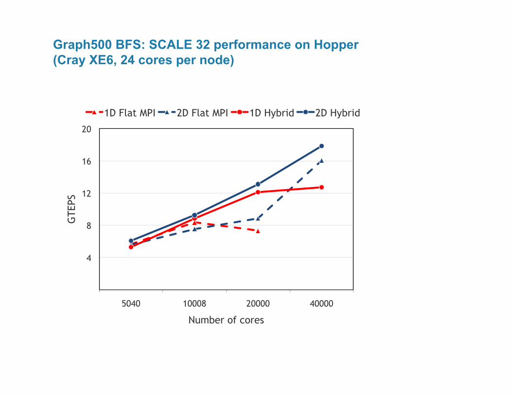
Graph500 BFS: SCALE 32 performance on Hopper (Cray XE6, 24 cores per node)
4
8
12
16
20
5040 10008 20000 40000
GTE
PS
Number of cores
1D Flat MPI 2D Flat MPI 1D Hybrid 2D Hybrid
Graph500 BFS: SCALE 32 communication time on Hopper (lower is better)
2
4
6
8
10
12
5040 10008 20000 40000
Com
m.
tim
e (s
econ
ds)
Number of cores
1D Flat MPI 2D Flat MPI 1D Hybrid 2D Hybrid
De novo Genome Assembly
• Genome Assembly: “a big jigsaw puzzle”
• De novo: Latin expression meaning “from the beginning” – No prior reference
organism – Computationally falls
within the NP-hard class of problems
De novo Genome Assembly
DNA extraction
Fragment the DNA
Clone into vectors Isolate vector DNA
Sequence the library
CTCTAGCTCTAA AGGTCTCTAA
AAGTCTCTAA AAGCTATCTAA
CTCTAGCTCTAAGGTCTCTAACTAAGCTAATCTAA
Genome Assembly
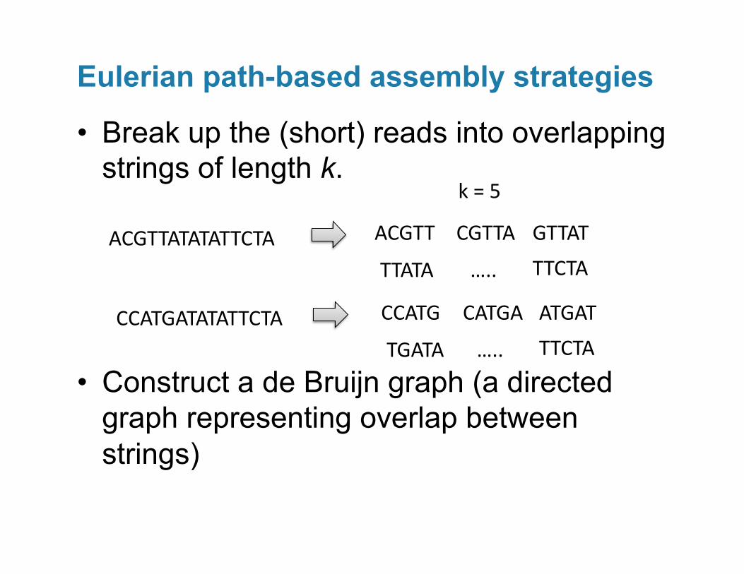
• Break up the (short) reads into overlapping strings of length k.
• Construct a de Bruijn graph (a directed graph representing overlap between strings)
Eulerian path-based assembly strategies
ACGTTATATATTCTA ACGTT CGTTA GTTAT
TTATA ….. TTCTA
k = 5
CCATGATATATTCTA CCATG CATGA ATGAT
TGATA ….. TTCTA
• Each (k-1)-mer represents a node in the graph • Edge exists between node a to b iff there exists a k-mer
such that its prefix is a and suffix is b.
• Traverse the graph (if possible, identifying an Eulerian path) to form contigs.
• However, correct assembly is just one of the many possible Eulerian paths.
de Bruijn graph-based Assembly
AAGACTCCGACTGGGACTTT AAG AGA GAC ACT CTT TTT
CTG TGG GGG
GGA
CTC TCC CCG CGA
ACTCCGACTGGGACTTTGAC TGA
Application: Identification of biomass-degrading Genes and Genomes from cow rumen
Image Source: Hess et al., Science 331(6016), 463-467, 2011.
Goal: Identify microbial enzymes that aid in deconstruction of plant polysaccharides. Cow rumen microbes known to be particularly effective In breaking down switchgrass.
• Two major complications for de novo assembly: – Likely uneven representation of organisms within a
sample – Likely polymorphisms between closely related
members in an environment • Assembly is difficult even if we have an estimate
of organism representation in a sample • If coverage is not known, Poisson likelihood
estimates used by isolate genome assemblers break down.
Metagenomes
• Given the challenges, what approach do we take?
• We can still construct the de Bruijn graph – Try out various values of k, use base quality information – Require parallel computation for dealing with the large data sizes
• Understand data set characteristics to suggest algorithmic changes in current assemblers – Can we automate selection of k? – What is the genome coverage like? – Can we predict the approximate size of the metagenome?
Towards designing a metagenome assembler
Steps in the new de Bruijn graph-based assembly scheme
FASTQ input data
Sequences aXer error resolu'on
1 Preprocessing
Determine appropriate value of k to use
2 Kmer spectrum
Preliminary de Bruijn graph construc'on
3
Vertex/edge compac'on (lossless transforma'ons)
4
Error resolu'on + further graph compac'on
5
Scaffolding 6
Compute and memory-intensive
• Process base quality information • Mark ambiguous bases
• Try to merge paired reads
• Write back filtered reads • Parallelization strategy: split input files into
“P” parts; each node processes its file independently – Predominantly I/O bound
1. Preprocessing
paired reads
Insert length of ~ 200bp
125bp 125bp
• Need a dictionary to track occurrences of each kmer
• Velvet uses a splay tree to track unique kmers – Splaying expensive for large data sizes;
maintaining an ordered set unnecessary when kmer updates are predominantly insert-only (“cow rumen” dataset)
• Alternative: Ingest all kmers, perform lexicographical sort
• Parallelization: enumerate kmers independently + one global sort to get kmer count
2. Kmer spectrum construction
Finding unique kmers: hashing vs sorting
0
500
1000
1500
2000
2500
3000
3500
1 2 3 4 5 6 7 8 9 10 11 12 13 14 15 16 17 18 19
Exec
utio
n tim
e (s
econ
ds)
# of reads (in millions)
Splay tree update time for a data set of 19.5 million (125 bp) reads (k=61)
Serial performance results on a 512 GB system (2.6 GHz Opteron processor)
51 GB memory
Serial sort, 18.6 GB memory 4.2x faster
• Store edges only, represent vertices (kmers) implicitly.