LARGE-SCALE RANDOM FEATURES FOR KERNEL REGRESSION Valero Laparra 1 , Diego Marcos Gonzalez 2 , Devis Tuia 2 and Gustau Camps-Valls 1 1 Image Processing Lab (IPL), Universitat de Val` encia, Spain, {valero.laparra,gustau.camps}@uv.es 2 University of Zurich, Switzerland, {diego.marcos, devis.tuia}@geo.uzh.ch ABSTRACT Kernel methods constitute a family of powerful machine learning algorithms, which have found wide use in remote sensing and geosciences. However, kernel methods are still not widely adopted because of the high computational cost when dealing with large scale problems, such as the inver- sion of radiative transfer models. This paper introduces the method of random kitchen sinks (RKS) for fast statistical retrieval of bio-geo-physical parameters. The RKS method allows to approximate a kernel matrix with a set of random bases sampled from the Fourier domain. We extend their use to other bases, such as wavelets, stumps, and Walsh expan- sions. We show that kernel regression is now possible for datasets with millions of examples and high dimensionality. Examples on atmospheric parameter retrieval from infrared sounders and biophysical parameter retrieval by inverting PROSAIL radiative transfer models with simulated Sentinel- 2 data show the effectiveness of the technique. 1. INTRODUCTION Kernel methods constitute an appropriate framework to ap- proach many statistical inference problems [1]. In the last decade these methods have replaced other techniques in many fields of science and engineering, and have become the new standard in remote sensing data analysis [2, 3]. Kernel meth- ods allow treating in the very same framework different prob- lems, from feature extraction [4] to classification [5] and re- gression [6]. The fundamental building block of the theory of kernel learning is the kernel function, which compares (pos- sibly complex) multidimensional data objects. In a nutshell, given n data points, all kernel methods have to operate with a squared (eventually huge) matrix of size n × n, which con- tains all pairwise sample similarities. Designing an appropri- ate kernel function that captures data dependencies is, nev- ertheless, not easy in general. Many approaches have been followed so far to tackle this problem: from learning the met- ric implicit in the kernel [7], to learning compositions of sim- pler kernels [8]. Selecting and optimizing a kernel function is We wish to thank Dr. Jochem Verrelst at the Image Processing Lab (IPL) in the Universitat de Val` encia (Spain) for preparing the data used in the sec- ond experiment. This paper has been partially supported by the Spanish Ministry of Econ- omy and Competitiveness under project TIN2012-38102-C03-01, and by the Swiss National Science Foundation under the grant PP00P2-150593. very challenging even with moderate amounts of data. Many efforts have been done to deliver large-scale versions of ker- nel machines able to work with several thousands of exam- ples. They typically resort to reduce the dimensionality of the problem by decomposing the kernel matrix using a subset of bases: for instance using Nystr¨ om eigendecompositions [9], sparse and low rank approximations [10, 4], or smart sample selection [11]. However, there is no clear evidence that these approaches work in general, given that they are mere approxi- mations to the kernel computed with all (possibly millions of) samples. In this paper, we explore an alternative pathway: rather than optimization we will follow randomization. While odd at a first glance, the approach has surprisingly yielded com- petitive results in the last years, being able to exploit many samples at a fraction of the computational cost. Besides its practical convenience, the approximation of the kernel with random bases is also theoretically consistent. The seminal work in [12] presented the randomization framework. Given a sample set {x i ∈ R d |i =1,...,n}, the idea is to approxi- mate the kernel function with an empirical kernel mapping of the form: k(x i , x j )= hφ(x i ), φ(x j )i≈ z(x i ) > z(x j ), where the implicit mapping φ(·) is replaced with an explicit (low-dimensional) feature mapping z(·) of dimension D. Consequently, one can simply transform the input with z, and then apply fast linear learning methods to approximate the corresponding nonlinear kernel machine. This approach not only provides extremely fast learning algorithms, but also good performance in the test phase: for a given test point x, instead of f (x)= ∑ n i=1 α i k(x i , x), which requires O(nd) operations, one simply does a linear projection f (x)= w > z, which requires O(D + d) operations. The question now is how to construct efficient and sensible z mappings. The work in [12] also introduced a particular technique to do so, called random kitchen sinks (RKS). The remainder of the paper is organized as follows. Sec- tion 2 reviews the RKS method, and introduces the different expansions used in this work. Section 3 presents and dis- cusses the experimental results in two challenging problems of bio-geo-physical parameter retrieval: atmospheric param- eter retrieval from infrared sounders such as IASI and inver- sion of PROSAIL radiative transfer models with Sentinel-2 simulated data. Section 4 concludes the paper.
Transcript
LARGE-SCALE RANDOM FEATURES FOR KERNEL REGRESSION
Valero Laparra1, Diego Marcos Gonzalez2, Devis Tuia2 and Gustau Camps-Valls1
1Image Processing Lab (IPL), Universitat de Valencia, Spain, {valero.laparra,gustau.camps}@uv.es2 University of Zurich, Switzerland, {diego.marcos, devis.tuia}@geo.uzh.ch
ABSTRACT
Kernel methods constitute a family of powerful machinelearning algorithms, which have found wide use in remotesensing and geosciences. However, kernel methods are stillnot widely adopted because of the high computational costwhen dealing with large scale problems, such as the inver-sion of radiative transfer models. This paper introduces themethod of random kitchen sinks (RKS) for fast statisticalretrieval of bio-geo-physical parameters. The RKS methodallows to approximate a kernel matrix with a set of randombases sampled from the Fourier domain. We extend their useto other bases, such as wavelets, stumps, and Walsh expan-sions. We show that kernel regression is now possible fordatasets with millions of examples and high dimensionality.Examples on atmospheric parameter retrieval from infraredsounders and biophysical parameter retrieval by invertingPROSAIL radiative transfer models with simulated Sentinel-2 data show the effectiveness of the technique.
1. INTRODUCTION
Kernel methods constitute an appropriate framework to ap-proach many statistical inference problems [1]. In the lastdecade these methods have replaced other techniques in manyfields of science and engineering, and have become the newstandard in remote sensing data analysis [2, 3]. Kernel meth-ods allow treating in the very same framework different prob-lems, from feature extraction [4] to classification [5] and re-gression [6]. The fundamental building block of the theory ofkernel learning is the kernel function, which compares (pos-sibly complex) multidimensional data objects. In a nutshell,given n data points, all kernel methods have to operate witha squared (eventually huge) matrix of size n× n, which con-tains all pairwise sample similarities. Designing an appropri-ate kernel function that captures data dependencies is, nev-ertheless, not easy in general. Many approaches have beenfollowed so far to tackle this problem: from learning the met-ric implicit in the kernel [7], to learning compositions of sim-pler kernels [8]. Selecting and optimizing a kernel function is
We wish to thank Dr. Jochem Verrelst at the Image Processing Lab (IPL)in the Universitat de Valencia (Spain) for preparing the data used in the sec-ond experiment.This paper has been partially supported by the Spanish Ministry of Econ-omy and Competitiveness under project TIN2012-38102-C03-01, and by theSwiss National Science Foundation under the grant PP00P2-150593.
very challenging even with moderate amounts of data. Manyefforts have been done to deliver large-scale versions of ker-nel machines able to work with several thousands of exam-ples. They typically resort to reduce the dimensionality of theproblem by decomposing the kernel matrix using a subset ofbases: for instance using Nystrom eigendecompositions [9],sparse and low rank approximations [10, 4], or smart sampleselection [11]. However, there is no clear evidence that theseapproaches work in general, given that they are mere approxi-mations to the kernel computed with all (possibly millions of)samples.
In this paper, we explore an alternative pathway: ratherthan optimization we will follow randomization. While oddat a first glance, the approach has surprisingly yielded com-petitive results in the last years, being able to exploit manysamples at a fraction of the computational cost. Besides itspractical convenience, the approximation of the kernel withrandom bases is also theoretically consistent. The seminalwork in [12] presented the randomization framework. Givena sample set {xi ∈ Rd|i = 1, . . . , n}, the idea is to approxi-mate the kernel function with an empirical kernel mapping ofthe form:
k(xi,xj) = 〈φ(xi),φ(xj)〉 ≈ z(xi)>z(xj),
where the implicit mapping φ(·) is replaced with an explicit(low-dimensional) feature mapping z(·) of dimension D.Consequently, one can simply transform the input with z,and then apply fast linear learning methods to approximatethe corresponding nonlinear kernel machine. This approachnot only provides extremely fast learning algorithms, but alsogood performance in the test phase: for a given test point x,instead of f(x) =
∑ni=1 αik(xi,x), which requires O(nd)
operations, one simply does a linear projection f(x) = w>z,which requires O(D + d) operations. The question now ishow to construct efficient and sensible z mappings. The workin [12] also introduced a particular technique to do so, calledrandom kitchen sinks (RKS).
The remainder of the paper is organized as follows. Sec-tion 2 reviews the RKS method, and introduces the differentexpansions used in this work. Section 3 presents and dis-cusses the experimental results in two challenging problemsof bio-geo-physical parameter retrieval: atmospheric param-eter retrieval from infrared sounders such as IASI and inver-sion of PROSAIL radiative transfer models with Sentinel-2simulated data. Section 4 concludes the paper.
2. KERNEL APPROXIMATION WITH RANDOMKITCHEN SINKS
2.1. Random kitchen sinks
Random kitchen sinks exploit a classical definition in har-monic analysis [12], by which a continuous kernel k(x,y) =k(x − y) on Rd is positive definite if and only if k is theFourier transform of a non-negative measure. If a shift-invariant kernel k is properly scaled, its Fourier transformp(ω) is a proper probability distribution. Defining the func-tion Cω(x) = ejω
>x, we obtain
k(x− y) =
∫Rd
p(ω)ejω>(x−y)dω = Eω[Cω(x)Cω(y)
∗],
so Cω(x)Cω(y)∗ is an unbiased estimate of k(x − y) when
ω is drawn from p. In our case, both p(ω) and k(x − y) arereal valued, what allows us to substitute the complex expo-nentials by cosines and to use zω(x)>zω(y), where zω(x) =√2cos(ω>x+ b), as an estimator of k(x− y) as long as ω is
drawn from p(ω) and b is drawn uniformly from [0, 2π]. Alsonote that zω(x)>zω(y) has expected value k(x,y) because ofthe sum of angles formula. Now, one can lower the varianceof the estimate of the kernel by concatenating D randomlychosen zω into one D-dimensional vector z and normalizingeach component by
√D. An illustrative example of how RKS
approximates k with random bases is given in Fig. 1.
RBF, ideal RKS, D = 1
RKS, D = 5 RKS, D = 1000
Fig. 1: Illustration of the effect of randomly sampling D bases fromthe Fourier domain on the kernel matrix. With sufficiently large D,the kernel matrix generated by RKS approximates that of the RBFkernel, at a fraction of the time.
2.2. RKS in practice
The RKS algorithm reduces to the following steps:
1. Draw D i.i.d. samples ω1, . . . , ωD ∈ Rd from p, andb1, . . . , bD ∈ R from the uniform distribution [0, 2π]
2. Construct the low-dimensional feature map:
z =√
2D [cos(ω>1 x+ b1), . . . , cos(ω
>Dx+ bD)]
3. Approximate the kernel function: k ≈ z>z, and asso-ciated kernel matrix, K = ZZ>
The method is very efficient in both speed and memory re-quirements, as shown in Table 1.
Table 1: Computational and memory costs for different approxi-mate kernel methods in problems with d dimensions, D features, nsamples.
Method Train time Test time Train mem Test memNaive [1] O(n2d) O(nd) O(nd) O(nd)
Low Rank [10] O(nDd) O(Dd) O(Dd) O(Dd)
RKS [12] O(nDd) O(Dd) O(Dd) O(Dd)
2.3. RKS beyond Fourier bases
The RKS algorithm can actually exploit other approximatingfunctions besides Fourier expansions. Note that actually anyshift-invariant kernel, i.e. k(x,y) = k(x − y), can be rep-resented using random cosine features. Randomly samplingdistribution functions impacts the definition of the corre-sponding reproducing kernel Hilbert space (rkHs): samplingthe Fourier bases with zω(x) =
√2 cos(ω>o x + b) actually
leads to the Gaussian RBF kernel k(x,y) = exp(−‖x −y‖2/(2σ2)), while a random stump (i.e. sigmoid-shapedfunctions) sampling defined by zω(x) = sign(x − ω) leadsto the kernel k(x,y) = 1 − 1
a‖x − y‖1. Another possibilityis to resort to binning bases functions, which partition theinput space using an axis-aligned grid, and assign a binaryindicator to each partition, which is shown to approximate aLaplacian kernel, k(x,y) = exp(−‖x−y‖1/(2σ2)) [12]. Inthis paper we will also explore the possibility of Walsh andthe Gabor basis functions widely used in signal and imageprocessing.
3. EXPERIMENTS
This paper presents experimental results on the use in RKS intwo remote sensing applications. We exploit several kitchensinks: the standard random Fourier basis functions, alongwith the Walsh, Haar, wavelets and stumps.
In this first experiment, we exploit random kernels in a chal-lenging regression problem in remote sensing: the estima-tion of atmospheric profiles from large scale hyperspectralinfrared sounders. Temperature and water vapor are atmo-spheric parameters of high importance for weather forecastand atmospheric chemistry studies [13]. Observations fromspaceborne high spectral resolution infrared sounding instru-ments can be used to calculate the profiles of such atmo-spheric parameters with unprecedented accuracy and verticalresolution [14]. In this work we focus on the data com-ing from the Infrared Atmospheric Sounding Interferometer(IASI), that provides radiances in 8461 spectral channels,between 3.62 and 15.5 µm with a spectral resolution of
(a) (b) (c)
0 500 1000 15003
3.5
4
4.5
5
5.5
#random features
RM
SE
LR
KRR (n=5000)
Fourier KRR
Walsh KRR
Wavelet KRR
Stump KRR
Sinc KRR
0 500 1000 150010
−2
10−1
100
101
102
103
#random featuresC
PU
tim
e [
sec
]
LR
KRR (n=5000)
Fourier KRR
Walsh KRR
Wavelet KRR
Stump KRR
Sinc KRR
3 3.5 4 4.5 5 5.510
−2
10−1
100
101
102
103
RMSE
CP
U t
ime
[se
c]
LR
KRR (n=5000)
Fourier KRR
Walsh KRR
Wavelet KRR
Stump KRR
Sinc KRR
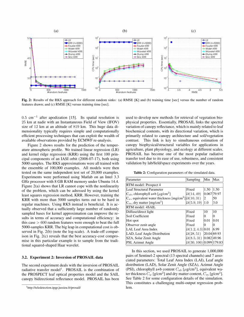
Fig. 2: Results of the RKS approach for different random sinks: (a) RMSE [K] and (b) training time [sec] versus the number of randomfeatures drawn; and (c) RMSE [K] versus training time [sec].
0.5 cm−1 after apodization [15]. Its spatial resolution is25 km at nadir with an Instantaneous Field of View (IFOV)size of 12 km at an altitude of 819 km. This huge data di-mensionality typically requires simple and computationallyefficient processing techniques that can exploit the wealth ofavailable observations provided by ECMWF re-analysis.
Figure 2 shows results for the prediction of the temper-ature atmospheric profile. We trained linear regression (LR)and kernel ridge regression (KRR) using the first 100 prin-cipal components of an IASI orbit (2008-07-17), both using5000 samples. The RKS approximations were all trained withthe ensemble of 100,000 examples. All models were thentested on the same independent test set of 20,000 examples.Experiments were performed using Matlab on an Intel 3.3GHz processor with 8 GB RAM memory under Ubuntu 14.4.Figure 2(a) shows that LR cannot cope with the nonlinearityof the problem, which can be adressed by using the kernelleast squares regression method, KRR. However, training theKRR with more than 5000 samples turns out to be hard inregular machines. Using RKS instead is beneficial. It is ac-tually observed that a sufficiently large number of randomlysampled bases for kernel approximation can improve the re-sults in terms of accuracy and computational efficiency: inthis case > 600 random features were enough to beat the full5000-samples KRR. The big leap in computational cost is ob-served in Fig. 2(b) (note the log-scale). A trade-off compar-ison in Fig. 2(c) reveals that the best accuracy-cost compro-mise in this particular example is to sample from the tradi-tional squared-shaped Haar wavelet.
3.2. Experiment 2: Inversion of PROSAIL data
The second experiment deals with the inversion of PROSAILradiative transfer model1. PROSAIL is the combination ofthe PROSPECT leaf optical properties model and the SAILcanopy bidirectional reflectance model. PROSAIL has been
1http://teledetection.ipgp.jussieu.fr/prosail/
used to develop new methods for retrieval of vegetation bio-physical properties. Essentially, PROSAIL links the spectralvariation of canopy reflectance, which is mainly related to leafbiochemical contents, with its directional variation, which isprimarily related to canopy architecture and soil/vegetationcontrast. This link is key to simultaneous estimation ofcanopy biophysical/structural variables for applications inagriculture, plant physiology, and ecology at different scales.PROSAIL has become one of the most popular radiativetransfer tool due to its ease of use, robustness, and consistentvalidation by lab/field/space experiments over the years.
Table 2: Configuration parameters of the simulated data.
In this section, we used PROSAIL to generate 1,000,000pairs of Sentinel-2 spectral (13 spectral channels) and 7 asso-ciated parameters: Total Leaf Area Index (LAI), Leaf angledistribution (LAD), Solar Zenit Angle (SZA), Azimut Angle(PSI), chlorophyll a+b content Cab [µg/cm2], equivalent wa-ter thicknessCw [g/cm2] and dry matter content,Cm [g/cm2].See Table 2 for some configuration details of the simulation.This constitutes a challenging multi-output regression prob-lem.
0 1000 20000.2
0.4
0.6
0.8
1
LAI
# features
No
rma
lize
d R
MSE
0 1000 20000.2
0.4
0.6
0.8
1
LAD
# features
No
rma
lize
d R
MSE
0 1000 20000.8
0.85
0.9
0.95
1
1.05
SZA
# features
No
rma
lize
d R
MSE
0 1000 20000.99
1
1.01
1.02
1.03
1.04
PSI
# features
No
rma
lize
d R
MSE
0 1000 20000
0.2
0.4
0.6
0.8
1
Cab
# features
No
rma
lize
d R
MSE
0 1000 20000.2
0.4
0.6
0.8
1
Cw
# features
No
rma
lize
d R
MSE
0 1000 20000
0.2
0.4
0.6
0.8
1
Cm
# features
No
rma
lize
d R
MSE
0 1000 200010
−2
100
102
104
# features
Co
st [
s]
LR
KRR, n=2000
RKS, n=400000
Fig. 3: RMSE results in the PROSAIL inversion experiment for theseven parameters and the computational cost (bottom right).
Figure 3 shows the obtained results for the inversion ofPROSAIL. We show both the normalized RMSE and the com-putational cost of a regularized linear regression, KRR andRKS. In all cases we predict the seven parameters with a sin-gle multiple-output regression model. We trained KRR with2,000 samples, and consequently trained RKS for a maximumof D = 2000. RKS employed 400,000 samples and cosinebasis. Several conclusions can be derived: 1) RKS yields ingeneral competitive performance versus KRR; and 2) RKSlargely improves predictions for LAD, SZA, and PSI estima-tion, while similar in accuracy to KRR for the rest of param-eters.
4. CONCLUSIONS
This paper explored the use of randomly-generated bases forlarge-scale kernel regression in remote sensing biophysicalparameter estimation. We exploited the approximation of thekernel function via random sampling from Fourier, wavelets,Walsh and stump functions. We showed results in two prob-lems. First we tackled a high-dimensional large scale prob-lem very common in remote sensing: the estimation of atmo-spheric profiles from large scale hyperspectral infrared sound-ing IASI radiances. Second, we explored RKS for the inver-sion of the widely used PROSAIL radiative transfer modelfor which we used 400,000 pairs of Sentinel-2 simulations.Both are multi-output problems. Results showed that we cantrain kernel regression models with several thousands of datapoints, which is not possible in standard kernel optimizationstrategies. The RKS model produced big gains in accuracyand computational efficiency.
We noted however that RKS has two shortcomings. First,the memory bottleneck is still present as one has to store theZ matrix, which is D × n, to compute the approximate ker-nel matrix, K = ZZ>. This will be addressed in the futurethrough low-rank and blocky approximation of Z. And sec-ond, other (sparser) bases can be more appropriate. In thiswork, we used the Walsh basis but results did not improvethose of standard Fourier bases. Alternatives to Hadamardexpansions, much in line of Fastfood [16], could eventuallyimprove further the results and efficiency.
5. REFERENCES
[1] J. Shawe-Taylor and N. Cristianini, Kernel Methods for PatternAnalysis, Cambridge University Press, 2004.
[2] G. Camps-Valls and L. Bruzzone, Eds., Kernel methods forRemote Sensing Data Analysis, Wiley & Sons, UK, Dec 2009.
[3] G. Camps-Valls, D. Tuia, L. Gomez-Chova, S. Jimenez, andJ. Malo, Eds., Remote Sensing Image Processing, Morgan &Claypool Publishers, LaPorte, CO, USA, Sep 2011.
[4] J. Arenas-Garcia, K. Petersen, G. Camps-Valls, and L.K.Hansen, “Kernel multivariate analysis framework for super-vised subspace learning: A tutorial on linear and kernel multi-variate methods,” Signal Processing Magazine, IEEE, vol. 30,no. 4, pp. 16–29, July 2013.
[5] G. Camps-Valls, D. Tuia, L. Bruzzone, and J. Atli Benedik-tsson, “Advances in hyperspectral image classification: Earthmonitoring with statistical learning methods,” Signal Process-ing Magazine, IEEE, vol. 31, no. 1, pp. 45–54, Jan 2014.
[6] G. Camps-Valls, J. Munoz and, L. Gomez, L. Guanter, andX. Calbet, “Nonlinear statistical retrieval of atmospheric pro-files from MetOp-IASI and MTG-IRS infrared sounding data,”IEEE Transactions on Geoscience and Remote Sensing, vol.50, no. 5, pp. 1759–1769, 2012.
[7] K.Q. Weinberger and G. Tesauro, “Metric learning for kernelregression,” in International Conference on Artificial Intelli-gence and Statistics, 2007, pp. 608–615.
[8] A. Rakotomamonjy, F.R. Bach, S. Canu, and Y. Grandvalet,“SimpleMKL,” Journal of Machine Learning Research, vol. 9,pp. 2491–2521, Nov. 2008.
[9] S. Kumar, M. Mohri, and A. Talwalkar, “Sampling methods forthe Nystrom method,” Journal of Machine Learning Research,vol. 13, pp. 981–1006, 2012.
[10] S. Fine and K. Scheinberg, “Efficient SVM training using low-rank kernel representations,” Journal of Machine Learning Re-search, vol. 2, pp. 243–264, 2001.
[11] A. Bordes, S. Ertekin, J. Weston, and L. Bottou, “Fast kernelclassifiers with online and active learning,” Journal of MachineLearning Research, vol. 6, pp. 1579–1619, 2005.
[12] Ali Rahimi and Benjamin Recht, “Random features for large-scale kernel machines,” in Neural Information Processing Sys-tems, 2007.
[13] K. N. Liou, An Introduction to Atmospheric Radiation, Aca-demic Press, Hampton, USA, 2nd edition, 2002.
[14] H. L. Huang, W. L. Smith, and H. M. Woolf, “Vertical resolu-tion and accuracy of atmospheric infrared sounding spectrom-eters,” Journal of Applied Meteorology, vol. 31, pp. 265–274,1992.
[15] D. Simeoni, C. Singer, and G. Chalon, “Infrared atmosphericsounding interferometer,” Acta Astronautica, vol. 40, pp. 113–118, 1997.
[16] Quoc Le, Tamas Sarlos, and Alex Smola, “Fastfood – approx-imating kernel expansions in loglinear time,” in InternationalConference on Machine Learning, 2013.


![KERNEL WARS: KERNEL-EXPLOITATION DEMYSTIFIED · –pGDI[(H & 0xffff)].nType == Windows Local GDI Kernel Memory Overwrite • Setting up a kernel debugging environment](https://static.documents.pub/doc/80x56/5c01a56009d3f252338ceb13/kernel-wars-kernel-exploitation-demystified-pgdih-0xffffntype-.jpg)


