Large-scale structure non-Gaussianities with modal methods (Ascona)

LARGE SCALE STRUCTURE

NON-GAUSSIANITIES

WITH MODAL METHODS

Marcel SchmittfullDAMTP, University of Cambridge

Collaborators: Paul Shellard, Donough Regan, James Fergusson

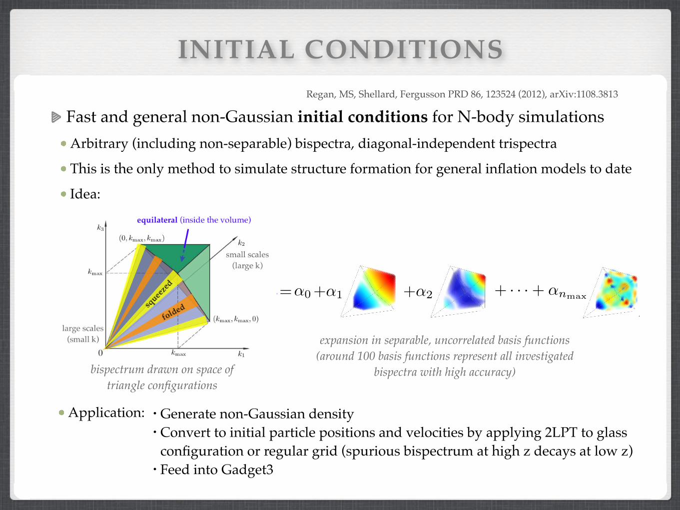
Based on 1108.3813, 1207.5678

LSS13, Ascona, 3 July 2013

PRIMORDIAL MOTIVATION

LSS = most promising window for non-Gaussianity after Planck (3d data; single field inflation can be ruled out with halo bias; BOSS, DES, Euclid, ...)

Local template/linear regime rather well understood

But: Effects beyond local template/linear regime not well studied

Dalal et al. 2008, Jeong/Komatsu 2009, Sefusatti et al. 2009-2012, Baldauf/Seljak/Senatore 2011, ...

Vacuum expectation value of a quantum field perturbation with inflationary Lagrangian

Free theory is Gaussian

Interacting theory is non-Gaussianpossible for all n, k-dependence characterises interactions

➟ Inflationary interactions are mapped to specific types of non-Gaussianity

h⌦|�'k1 · · · �'kn |⌦i =(determined by 2-point function, n even,

0, n odd.

h⌦|�'k1 · · · �'kn |⌦i 6= 0

h⌦|�'k1 · · · �'kn |⌦i =RD[�']�'k1 · · · �'knexp(i

RC L(�'k))R

D[�']exp(iRC L(�'k))

L ⇠ �'2 ) eiRC L

L ⇠ �'3, �'4, . . . ) eiRC L

�' L

Complementary late-time motivation for LSS bispectrum:

LATE-TIME MOTIVATION

Fry 1994Verde et al. 1997-2002Scoccimarro et al. 1998Sefusatti et al. 2006

But: No LSS bispectrum pipeline

Complicated modelling (non-linear DM, bias, RSD, correlations, systematics, ...)

Ph(k) ⇡ b21P�(k) Bh(k1, k2, k3) ⇡ b31B�(k1, k2, k3) + b21b2(P�(k1)P�(k2) + perms)

Halo power spectrum Halo bispectrum

Break b1-!m degeneracy, i.e. can measure !m from LSS alone

Measure b2

Cannot distinguish rescaling of P" from b1

➟ b1-!m degeneracy

From (naive) we get�h(x) ⇠ b1�(x) +1

2b2�(x)

2 + · · ·

BISPECTRUM

BispectrumPrimary diagnostic for non-Gaussianity because vanishes for Gaussian perturbations

Defined for closed triangles (statistical homogeneity and isotropy)

h�(k1)�(k2)�(k3)i = (2⇡)3�D(k1 + k2 + k3)fNLB�(k1, k2, k3)

non-linear amplitude

bispectrum

k1 k2

k3sum of the two smaller sides ≥ longest side

(every point corresponds to a triangle config.)

)k3

kmax

kmax k1

k2

Bispectrum domain = ‘tetrapyd’(=space of triangle configurations)

BISPECTRUM SHAPES

)

k3

kmax

kmax k1

k2

Squeezed triangles (local shape)

Arises in multifield inflation; detection would rule out all single field models!

Different inflation models induce different momentum dependencies (shapes) of B�(k1, k2, k3)

k2 ⇡ k3 � k1

k1k2

k3

Equilateral triangles

k1 ⇡ k2 ⇡ k3

k3

kmax

kmax k1

k2

k3

kmax

kmax k1

k2

Typically higher derivative kinetic terms, e.g. DBI inflation

Folded triangles

k3 = 2k1 = 2k2

k2

k3

k1

E.g. non-Bunch-Davies vacuum

bispectrum drawn on space of triangle configurations

INITIAL CONDITIONS

Fast and general non-Gaussian initial conditions for N-body simulationsArbitrary (including non-separable) bispectra, diagonal-independent trispectra

This is the only method to simulate structure formation for general inflation models to date

Idea:

↵0= +↵1 +↵2

Note: Actually we plot an orthonormalised version of hereQn

+ · · ·+ ↵nmax

WB

bispectrum drawn on space of triangle configurations

expansion in separable, uncorrelated basis functions(around 100 basis functions represent all investigated

bispectra with high accuracy)

Regan, MS, Shellard, Fergusson PRD 86, 123524 (2012), arXiv:1108.3813

• Generate non-Gaussian density• Convert to initial particle positions and velocities by applying 2LPT to glass

configuration or regular grid (spurious bispectrum at high z decays at low z)• Feed into Gadget3

Application:

Simplest case: local non-Gaussianity

General case: arbitrary bispectrum

Wagner et al 2010

(=2 in local case)WB(k, k0, k00) ⌘ B�(k, k0, k00)

P�(k)P�(k0) + P�(k)P�(k00) + P�(k0)P�(k00)

INITIAL CONDITIONS: MATHS

Aim: Create non-Gaussian field

B�

Fergusson, Regan, Shellard PRD 86, 063511 (2012), arXiv: 1008.1730Regan, MS, Shellard, Fergusson PRD 86, 123524 (2012), arXiv:1108.3813

Requires ~N6 operations in general, but only ~N3 operations if WB was separable:

WB(k, k0, k00) = f1(k)f2(k

0)f3(k00) + perms

full field Gaussian �(x) = �G(x) + �NG(x)

non-Gaussian part

�(x) = �G(x) + fNL(�2G(x)� h�2

Gi)

Expanding WB in separable basis functions gives N3 scaling for any* bispectrum

*Scoccimarro and Verde groups try to rewrite WB analytically in separable form; this works sometimes, but not in general

�NG(k) =fNL

2

Zd3k0d3k00

(2⇡)3�D(k� k0 � k00)WB(k, k

0, k00)�G(k0)�G(k

00)

N =#ptcles

dim⇠ 1000

BISPECTRUM ESTIMATION

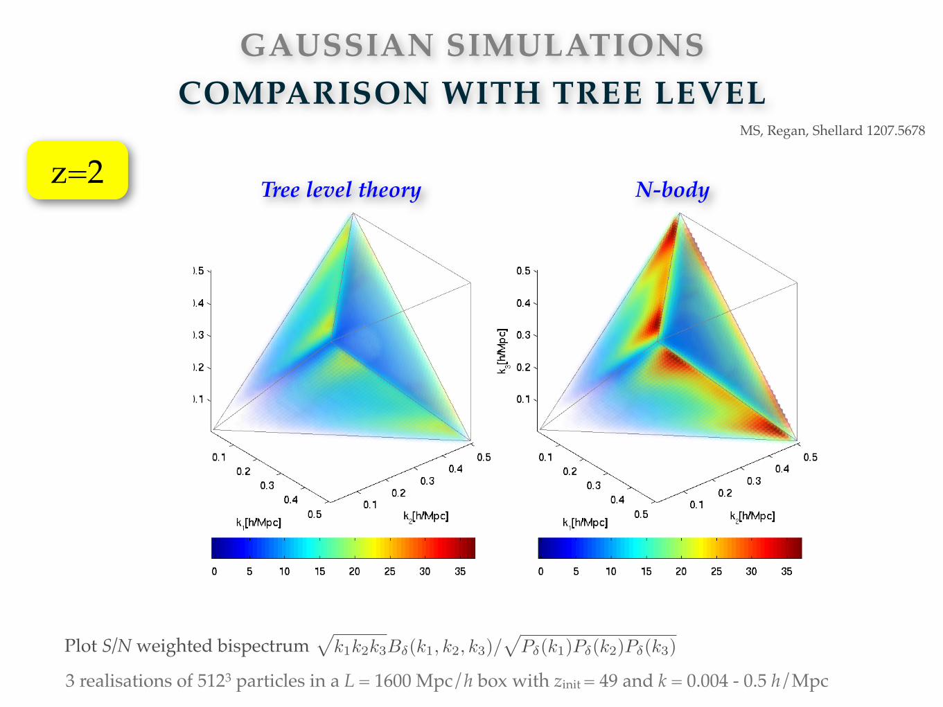
Fast and general bispectrum estimator for N-body simulations MS, Regan, Shellard 1207.5678

Measure ~100 fNL amplitudes of separable basis shapes, combine them to reconstruct the full bispectrum

Scales like 100xN3 instead of N6, where N~1000 (speedup by factor ~107)

Can estimate bispectrum whenever power spectrum is typically measured

Validated against PT at high z

Useful compression to ~100 numbers

Automatically includes all triangles

Loss of total S/N due to truncation of basis is only a few percent (could be improved with larger basis; for ~N3 basis functions the estimator would be exact)

Theory

Expansion of theory

N-body

Gravity Excess bispectrum for local NGz=30

http://arxiv.org/abs/1207.5678


BISPECTRUM ESTIMATION: MATHSFergusson, Shellard et al. 2009-2012MS, Regan, Shellard 1207.5678

Likelihood for fNL given a density perturbation δk

Maximise w.r.t. fNL (given a theoretical bispectrum )

Requires ~N6 operations in general, but only ~N3 operations if was separable

➟ Measure amplitudes of separable basis functions

➟ Combine them to reconstruct full bispectrum from the data:

L /Z

d3k1

(2⇡)3d3k2

(2⇡)3d3k3

(2⇡)3

2

641�1

6h�k1�k2�k3i| {z }

/fNLB�

@

@�k1

@

@�k2

@

@�k3

+ · · ·

3

751p

detC

Y

ij

e�12 �

⇤ki

(C�1)ij�kj

/ P�

f̂Btheo

�NL =

1

NfNL

Zd3k

1

(2⇡)3d3k

2

(2⇡)3d3k

3

(2⇡)3(2⇡)3�D(k

1

+ k2

+ k3

)Btheo

� (k1

, k2

, k3

)�k1

�k2

�k3

P�(k1)P�(k2)P�(k3)

Btheo

�

Btheo

�

where , , �Rn ⌘

X

m

�nm�Qm Mr(x) ⌘

Zd3k

(2⇡)3eikx

qr(k)�obskp

kP�(k)�Qm ⌘

Zd3xMr(x)Ms(x)Mt(x)

B̂(k1, k2, k3) =X

n

�Rn

sP�(k1)P�(k2)P�(k3)

k1k2k3Rn(k1, k2, k3)

depends on data



GAUSSIAN

SIMULATIONS

MS, Regan, Shellard 1207.5678

3 realisations of 5123 particles in a L = 1600 Mpc/h box with zinit = 49 and k = 0.004 - 0.5 h/Mpc

Plot S/N weighted bispectrumpk1k2k3B�(k1, k2, k3)/

pP�(k1)P�(k2)P�(k3)

z=30 Tree level theory N-body

GAUSSIAN SIMULATIONSCOMPARISON WITH TREE LEVEL






pP�(k1)P�(k2)P�(k3)

Tree level theory N-bodyz=2







pP�(k1)P�(k2)P�(k3)

Tree level theory N-bodyz=0




GAUSSIAN SIMULATIONSON SMALL SCALES




pP�(k1)P�(k2)P�(k3)

N-body N-body N-body

z=1 z=0z=2




DM density

GAUSSIAN SIMULATIONSCOMPARISON WITH DARK MATTER

5123 particles in a L = 400 Mpc/h box with zinit = 49 and k = 0.016 - 2 h/Mpc

Plot DM density in (40 Mpc/h)3 subbox and bispectrum signalpk1k2k3B�(k1, k2, k3)/

pP�(k1)P�(k2)P�(k3)

DM bispectrum

22

(a) Dark matter, z = 4 (b) Bispectrum signal, z = 4

(c) Dark matter, z = 2 (d) Bispectrum signal, z = 2

(e) Dark matter, z = 0 (f) Bispectrum signal, z = 0

Figure 10. Left: Dark matter distribution in a (40Mpc/h)3 subbox of one of the G512

400

simulations at redshifts z = 4, 2 and 0, from topto bottom. Right: Measured (signal to noise weighted) bispectrum in the range 0.016h/Mpc k 2h/Mpc, averaged over the simulationon the left and two additional seeds.

40 Mpc/h40

Mpc/h

22





400


z=4




DM density




pP�(k1)P�(k2)P�(k3)

DM bispectrum

22





400


40 Mpc/h40

Mpc/h

22





400


z=2




DM density




pP�(k1)P�(k2)P�(k3)

22





400


40 Mpc/h40

Mpc/h

22





400


z=0DM bispectrum



GAUSSIAN SIMULATIONSSUMMARY

Summary Gaussian N-body simulations

z=4

z=0

DM density DM bispectrum signal

pancakes

enhanced equilateral

filaments & clusters

flattened


Measured gravitational DM bispectrum for all triangles down to k=2hMpc-1

Non-linearities mainly enhance ‘constant’ 1-halo bispectrum

Bispectrum characterises 3d DM structures like pancakes, filaments, clusters

Self-similarity(constant contribution appears towards late times at fixed length scale, and towards small scales at fixed time)



NON-GAUSSIAN

SIMULATIONS

Tree level theory N-body

3 realisations of 5123 particles in a L = 1600 Mpc/h box with zinit = 49 and k = 0.004-0.5 h/Mpc, fNL=10

Plot S/N weighted excess bispectrumpk1k2k3B�(k1, k2, k3)/

pP�(k1)P�(k2)P�(k3)

z=30

LOCAL NON-GAUSSIAN SIMSMS, Regan, Shellard 1207.5678






pP�(k1)P�(k2)P�(k3)

z=2







pP�(k1)P�(k2)P�(k3)

z=0




OTHER SHAPES

Excess DM bispectra for other non-Gaussian initial conditions

multiple fields higher derivative operators non-standard vacuum


z=0, kmax=0.5hMpc-1, 5123 particlesNon-linear regime:

Tree level shape is enhanced by non-linear power spectrum

Additional ~constant contribution to bispectrum signal

Quantitative characterisation with cumulative S/N and 3d shape correlations in 1207.5678

multiple fields(local)

higher derivatives(equilateral)

non-standard vacuum(flattened)



Introduce scalar product , shape correlation and norm C

hBi, Bjiest ⌘V

⇡

Z

VB

dk1dk2dk3k1k2k3Bi(k1, k2, k3)Bj(k1, k2, k3)

P�(k1)P�(k2)P�(k3)

h·, ·iest

C(Bi, Bj) ⌘hBi, Bjiestp

hBi, BiiesthBj , Bjiest2 [�1, 1]

if then estimator for cannot find any and vice versa

Babich et al. 2004, Fergusson, Regan, Shellard 2010

||B|| ⌘phB,Biest

||B||

total integrated S/N

|C(B1, B2)| ⌧ 1B1

B2

) hf̂Btheo

NL

i = C(Bdata

� , Btheo

� )||Bdata

� ||||Btheo

� ||projection of data on theory

SIMILARITY OF SHAPES

f local

NL

= 10

Btheo

local

B̂NG{NG initial conditions with

10

20

30

40

flo

cN

L

k ! [ 0.0039, 0.5]h/Mpck ! [ 0.0039, 0.25]h/Mpck ! [ 0.0039, 0.13]h/Mpc

0

50

100F̄

B̂N

GN

L

1

10

||B̂

NG||

0.6

0.8

1

C! !, th" 0 .9613

C ",!

!

1 10

0.6

0.8

1

C NG

,G

1 + z

f̂ local

NL

timez=49today

C(B̂NG

, Blocal

)

Btheo

local

B̂NG

Btheo

local

B̂NG}

C(B̂NG, B̂Gauss)

B̂NG

B̂Gauss

||B|| / F̄NL


TIME SHIFT MODEL

Time shift model

Non-Gaussian universe evolves slightly faster (or slower) than Gaussian universe

Halos form earlier (later) in presence of primordial non-Gaussianity

Primordial non-Gaussianity gives growth of the 1-halo bispectrum a ‘headstart’ (or delay)

1-halobispectrum

at z

1-halobispectrum

at z+Δz

Gaussian universeNon-Gaussian universe

=


Motivates simple form of non-Gaussian excess bispectrum:

BNG� =

rPNL

� (k1)PNL� (k2)P

NL� (k3)

P�(k1)P�(k2)P�(k3)B�(k1, k2, k3)

| {z }perturbative with non-linear power

+c�z@z[Dnh

(z)](k1 + k2 + k3)⌫

| {z }time shifted 1-halo term

See Valageas for similar philosophy in Gaussian case (combing PT+halo model)



FITTING FORMULAE

Simple fitting formulae for grav. and primordial DM bispectrum shapesValid at 0 ≤ z ≤ 20, k ≤ 2hMpc-1 3d shape correlation with measured shapes is ≥ 94.4% at 0 ≤ z ≤ 20 and ≥ 98 % at z=0 (≥ 99.8% for gravity at 0 ≤ z ≤ 20)

Only ~3 free parameters per inflation model (local, equilateral, flattened, [orthogonal])


Overall amplitude needs to be rescaled by (poorly understood) time-dependent prefactor;extends Gil-Marin et al formula to smaller scales and NG ICs

⌫ ⇡ �1.7

BNG� =

rPNL

� (k1)PNL� (k2)P

NL� (k3)

P�(k1)P�(k2)P�(k3)B�(k1, k2, k3)

| {z }perturbative with non-linear power

+c�z@z[Dnh

(z)](k1 + k2 + k3)⌫

| {z }time shifted 1-halo term

26

100

101

101

102

103

104

1 + z

kBk

(a) Gaussian, kmax

= 0.5h/Mpc

100

101

102

103

104

105

1 + z

kBk

(b) Gaussian, kmax

= 2h/Mpc

Figure 15. Motivation for using the growth function D̄ in the simple fitting formula (64). The arbitrary weight w(z) in Bopt

� =

Bgrav

�,NL

+w(z)(k1

+ k2

+ k3

)⌫ is determined analytically such that C(B̂� , Bopt

� ) is maximal (for ⌫ = �1.7). We plot kBgrav

�,NL

k (black dotted),

kw(z)(k1

+ k2

+ k3

)⌫k (green) and Bgrav

�,const (black dashed) as defined in (14) with fitting parameters given in Table IV, illustrating that

w(z) = c1

D̄nh (z) is a good approximation. The continuous black and red curves show kBfit

� k from (64) and the estimated bispectrum size

kB̂�k, respectively. The overall normalisation can be adjusted with Nfit

as explained in the main text.

Simulation L[Mpc

h

] c1,2 n(prim)

h minz20

C�,↵ C�,↵(z=0)

G512g 1600 4.1⇥ 106 7 99.8% 99.8%

Loc10 1600 2⇥ 103 6 99.7% 99.8%

Eq100 1600 8.6⇥ 102 6 97.9% 99.4%

Flat10 1600 1.2⇥ 104 6 98.8% 98.9%

Orth100 1600 �3.1⇥ 102 5.5 91.0% 91.0%

G512

400

400 1.0⇥ 107 8 99.8% 99.8%

Loc10512400

400 2⇥ 103dD/da 7 98.2% 99.0%

Eq100512400

400 8.6⇥102dD/da 7 94.4% 97.9%

Flat10512400

400 1.2⇥104dD/da 7 97.7% 99.1%

Orth100512400

400 �2.6⇥ 102 6.5 97.3% 98.9%

Table IV. Fitting parameters c1

and nh for the fit (64) ofthe matter bispectrum for Gaussian initial conditions (sim-ulations G512g and G512

400

) and c2

and nprim

h for the fit (69)of the primordial bispectrum (58). The two columns on theright show the minimum shape correlation with the mea-sured (excess) bispectrum in N -body simulations, which wasmeasured at redshifts z = 49, 30, 20, 10, 9, 8, . . . , 0, and theshape correlation at z = 0. For the equilateral case the mini-mum shape correlation can be improved to 99.4% if the term4.6 ⇥ 10�5f

NL

D̄(z)0.5⇥2P�(k1)P�(k2)F

(s)2

(k1

,k2

) + 2 perms⇤

is added to (69).

information. All we require is the time dependence orgrowth rate of the bispectrum amplitude. As a first step,the fitting formula (65) can be normalised to the mea-sured bispectrum size by multiplying it with the normal-isation factor

Nfit ⌘ kB̂kkBfit

� k , (66)

which is shown by the dotted line in the lower panels ofFig. 16. While it varies with redshift between 0.7 and1.4 for kmax = 2h/Mpc, it deviates by at most 8% fromunity for kmax = 0.5h/Mpc. The lower panels also showthe measured integrated bispectrum size kB̂k and thetwo individual contributions to (64) when the normalisa-tion factor Nfit is included. These quantities are dividedby kBgrav

�,NLk for convenience. At high redshifts the totalbispectrum size is essentially given by the contributionfrom Bgrav

�,NL, which equals the tree level prediction for thegravitational bispectrum in this regime. The contribu-tion from Bconst

� dominates at z 2 for kmax = 2h/Mpcwhen filamentary and spherical nonlinear structures areapparent. A similar transition can be seen at later timeson larger scales in Fig. 16a, indicating self-similar be-haviour.

It is worth noting that the high integrated corre-lation between the simple fit (64) and measurementsdoes not imply that all triangle configurations agree per-fectly and sub-percent level di↵erences between shapecorrelations can in principle contain important informa-tion, e.g. about the observationally relevant squeezedlimit which only makes a small contribution to the to-tal tetrapyd integral over the signal-to-noise weighteddark matter bispectrum. However, if we observed thedark matter bispectrum directly, these shapes would behard to distinguish because the shape correlation con-tains the signal-to-noise weighting. Modified shape cor-relation weights and additional basis functions have beenused for better quantitative comparison of the squeezedlimit of dark matter bispectra, but this is left for a futurepublication.

Quality of fit:all z z=0

26

100

101

101

102

103

104

1 + z

kBk

(a) Gaussian, kmax

= 0.5h/Mpc

100

101

102

103

104

105

1 + z

kBk

(b) Gaussian, kmax

= 2h/Mpc

Figure 15. Motivation for using the growth function D̄ in the simple fitting formula (64). The arbitrary weight w(z) in Bopt

� =

Bgrav

�,NL

+w(z)(k1

+ k2

+ k3

)⌫ is determined analytically such that C(B̂� , Bopt

� ) is maximal (for ⌫ = �1.7). We plot kBgrav

�,NL

k (black dotted),

kw(z)(k1

+ k2

+ k3

)⌫k (green) and Bgrav

�,const (black dashed) as defined in (14) with fitting parameters given in Table IV, illustrating that

w(z) = c1

D̄nh (z) is a good approximation. The continuous black and red curves show kBfit

� k from (64) and the estimated bispectrum size

kB̂�k, respectively. The overall normalisation can be adjusted with Nfit

as explained in the main text.

Simulation L[Mpc

h

] c1,2 n(prim)

h minz20

C�,↵ C�,↵(z=0)

G512g 1600 4.1⇥ 106 7 99.8% 99.8%

Loc10 1600 2⇥ 103 6 99.7% 99.8%

Eq100 1600 8.6⇥ 102 6 97.9% 99.4%

Flat10 1600 1.2⇥ 104 6 98.8% 98.9%

Orth100 1600 �3.1⇥ 102 5.5 91.0% 91.0%

G512

400

400 1.0⇥ 107 8 99.8% 99.8%

Loc10512400

400 2⇥ 103dD/da 7 98.2% 99.0%

Eq100512400

400 8.6⇥102dD/da 7 94.4% 97.9%

Flat10512400

400 1.2⇥104dD/da 7 97.7% 99.1%

Orth100512400

400 �2.6⇥ 102 6.5 97.3% 98.9%

Table IV. Fitting parameters c1

and nh for the fit (64) ofthe matter bispectrum for Gaussian initial conditions (sim-ulations G512g and G512

400

) and c2

and nprim

h for the fit (69)of the primordial bispectrum (58). The two columns on theright show the minimum shape correlation with the mea-sured (excess) bispectrum in N -body simulations, which wasmeasured at redshifts z = 49, 30, 20, 10, 9, 8, . . . , 0, and theshape correlation at z = 0. For the equilateral case the mini-mum shape correlation can be improved to 99.4% if the term4.6 ⇥ 10�5f

NL

D̄(z)0.5⇥2P�(k1)P�(k2)F

(s)2

(k1

,k2

) + 2 perms⇤

is added to (69).

information. All we require is the time dependence orgrowth rate of the bispectrum amplitude. As a first step,the fitting formula (65) can be normalised to the mea-sured bispectrum size by multiplying it with the normal-isation factor

Nfit ⌘ kB̂kkBfit

� k , (66)

which is shown by the dotted line in the lower panels ofFig. 16. While it varies with redshift between 0.7 and1.4 for kmax = 2h/Mpc, it deviates by at most 8% fromunity for kmax = 0.5h/Mpc. The lower panels also showthe measured integrated bispectrum size kB̂k and thetwo individual contributions to (64) when the normalisa-tion factor Nfit is included. These quantities are dividedby kBgrav

�,NLk for convenience. At high redshifts the totalbispectrum size is essentially given by the contributionfrom Bgrav

�,NL, which equals the tree level prediction for thegravitational bispectrum in this regime. The contribu-tion from Bconst

� dominates at z 2 for kmax = 2h/Mpcwhen filamentary and spherical nonlinear structures areapparent. A similar transition can be seen at later timeson larger scales in Fig. 16a, indicating self-similar be-haviour.

It is worth noting that the high integrated corre-lation between the simple fit (64) and measurementsdoes not imply that all triangle configurations agree per-fectly and sub-percent level di↵erences between shapecorrelations can in principle contain important informa-tion, e.g. about the observationally relevant squeezedlimit which only makes a small contribution to the to-tal tetrapyd integral over the signal-to-noise weighteddark matter bispectrum. However, if we observed thedark matter bispectrum directly, these shapes would behard to distinguish because the shape correlation con-tains the signal-to-noise weighting. Modified shape cor-relation weights and additional basis functions have beenused for better quantitative comparison of the squeezedlimit of dark matter bispectra, but this is left for a futurepublication.



CONCLUSIONSConclusions

Efficient and general non-Gaussian N-body initial conditions

Fast estimation of full bispectrum

new standard diagnostic alongside power spectrum

Tracked time evolution of the DM bispectrum in a large suite of non-Gaussian N-body simulations

Time shift model for effect of primordial non-Gaussianity

New fitting formulae for gravitational and primordial DM bispectra

See 1108.3813 (initial conditions) 1207.5678 (rest)

COMPARISON WITH OTHER ESTIMATORS

Brute force bispectrum estimator

➟ Slow (107 times slower for 10003 simulation)

Taking only subset of triangle configurations/orientations

➟ Non-optimal estimator: Throw away data (instead, we compress theory domain, not data domain; and we quantify lost S/N~few %)

Binning

➟ Same as our estimator if basis functions are taken as top-hats

➟ But: Not known how much signal is lost with binning (our monomial basis looses few %)

Correlations between triangles and with power spectrum

➟ Potentially easier to get correlations for 100 than for full 3d bispectrum shape

Comparison with theory

➟ Easier with 100 than for full 3d bispectrum shape

Experimental realism:

➟ Need to try... (Planck started with ~7 bispectrum estimators, 3 survived)

�Rn

�Rn

Date post:	30-Jul-2015
Category:	Science
Upload:	marcel-schmittfull
View:	75 times
Download:	0 times

Large-scale structure non-Gaussianities with modal methods (Ascona)

Science