1 Large System Analysis of Linear Precoding in Correlated MISO Broadcast Channels under Limited Feedback Sebastian Wagner, Member, IEEE, Romain Couillet, Member, IEEE, M´ erouane Debbah, Senior Member, IEEE, and Dirk T. M. Slock, Fellow, IEEE Abstract—In this paper, we study the sum rate performance of zero-forcing (ZF) and regularized ZF (RZF) precoding in large MISO broadcast systems under the assumptions of imperfect channel state information at the transmitter and per-user channel transmit correlation. Our analysis assumes that the number of transmit antennas M and the number of single-antenna users K are large while their ratio remains bounded. We derive deterministic approximations of the empirical signal-to- interference plus noise ratio (SINR) at the receivers, which are tight as M,K →∞. In the course of this derivation, the per-user channel correlation model requires the development of a novel deterministic equivalent of the empirical Stieltjes transform of large dimensional random matrices with generalized variance profile. The deterministic SINR approximations enable us to solve various practical optimization problems. Under sum rate maximization, we derive (i) for RZF the optimal regularization parameter, (ii) for ZF the optimal number of users, (iii) for ZF and RZF the optimal power allocation scheme and (iv) the optimal amount of feedback in large FDD/TDD multi-user systems. Numerical simulations suggest that the deterministic approximations are accurate even for small M,K. Index Terms—Broadcast channel, linear precoding, limited feedback, multi-user systems, random matrix theory. I. I NTRODUCTION T HE pioneering work in [1] and [2] revealed that the capacity of a point-to-point (single-user (SU)) multiple- input multiple-output (MIMO) channel can potentially in- crease linearly with the number of antennas. However, practi- cal implementations quickly demonstrated that in most propa- gation environments the promised capacity gain of SU-MIMO is unachievable due to antenna correlation and line-of-sight components [3]. In a multi-user (MU) scenario, the inherent problems of SU-MIMO transmission can largely be overcome by exploiting multi-user diversity, i.e., sharing the spatial dimension not only between the antennas of a single receiver, but among multiple (non-cooperative) users. The underlying channel for MU-MIMO transmission is referred to as the S. Wagner is with ST-ERICSSON, Sophia-Antipolis R. Couillet is with SUP ´ ELEC, Gif sur Yvette, France, e- mail:[email protected]. S. Wagner and D.T.M. Slock are with EURECOM, Sophia- Antipolis, 06904, Route des Crˆ etes, B.P. 193, France, e- mail:{sebastian.wagner, dirk.slock}@eurecom.fr. M. Debbah is with the Alcatel-Lucent Chair on Flexible Radio, SUP ´ ELEC, Gif sur Yvette, France e-mail: [email protected]. This research has been partially supported by EU NoE Newcom++ and ANR project SESAME MIMO broadcast channel (BC) or MU downlink channel. Al- though much more robust to channel correlation, the MIMO- BC suffers from inter-user interference at the receivers which can only be efficiently mitigated by appropriate (i.e., channel- aware) pre-processing at the transmitter. It has been proved that dirty-paper coding (DPC) is a capacity achieving precoding strategy for the Gaussian MIMO- BC [4]–[8]. However, the DPC precoder is non-linear and to this day too complex to be implemented efficiently in practical systems. It has been shown in [4], [9]–[11], that suboptimal linear precoders can achieve a large portion of the BC rate region while featuring low computational complexity. Thus, a lot of research has recently focused on linear precoding strategies. In general, the rate maximizing linear precoder has no explicit form. Several iterative algorithms have been proposed in [12], [13], but no global convergence has been proved. Still, these iterative algorithms have a high computational complexity which motivates the use of further suboptimal linear transmit filters (i.e., precoders), by imposing more structure into the filter design. A straightforward technique is to precode by the inverse of the channel. This scheme is referred to as channel inversion or zero-forcing (ZF) [4]. Although [9], [12], [13] assume perfect channel state in- formation at the transmitter (CSIT) to determine theoretically optimal performance, this assumption is untenable in practice. It is indeed a particularly strong assumption, since the per- formance of all precoding strategies is crucially depending on the CSIT quality. In practical systems, the transmitter has to acquire the channel state information (CSI) of the downlink channel by feedback signaling from the uplink. Since in practice the channel coherence time is finite, the information of the instantaneous channel state is inherently incomplete. For this reason, a lot of research has been carried out to understand the impact of imperfect CSIT on the system behavior, see [14] for a recent survey. In this contribution, we focus on the multiple-input single- output (MISO) BC, where a central transmitter equipped with M antennas communicates with K single-antenna non- cooperative receivers. We assume M ≥ K, i.e., we do not account for user scheduling, and consider ZF and regularized ZF (RZF) precoding under imperfect CSIT (modeled as a weighted sum of the true channel plus independent noise) as well as per-user channel correlation, i.e., the vector channel h k ∈ C M of user k (k =1,...,K) satisfies E[h k ]=0
Transcript
1
Large System Analysis of Linear Precoding inCorrelated MISO Broadcast Channels under
Abstract—In this paper, we study the sum rate performance ofzero-forcing (ZF) and regularized ZF (RZF) precoding in largeMISO broadcast systems under the assumptions of imperfectchannel state information at the transmitter and per-user channeltransmit correlation. Our analysis assumes that the numberof transmit antennas M and the number of single-antennausers K are large while their ratio remains bounded. Wederive deterministic approximations of the empirical signal-to-interference plus noise ratio (SINR) at the receivers, which aretight as M,K → ∞. In the course of this derivation, the per-userchannel correlation model requires the development of a noveldeterministic equivalent of the empirical Stieltjes transform oflarge dimensional random matrices with generalized varianceprofile. The deterministic SINR approximations enable us tosolve various practical optimization problems. Under sum ratemaximization, we derive (i) for RZF the optimal regularizationparameter, (ii) for ZF the optimal number of users, (iii) forZF and RZF the optimal power allocation scheme and (iv)the optimal amount of feedback in large FDD/TDD multi-usersystems. Numerical simulations suggest that the deterministicapproximations are accurate even for small M,K.
Index Terms—Broadcast channel, linear precoding, limitedfeedback, multi-user systems, random matrix theory.
I. INTRODUCTION
THE pioneering work in [1] and [2] revealed that thecapacity of a point-to-point (single-user (SU)) multiple-
input multiple-output (MIMO) channel can potentially in-crease linearly with the number of antennas. However, practi-cal implementations quickly demonstrated that in most propa-gation environments the promised capacity gain of SU-MIMOis unachievable due to antenna correlation and line-of-sightcomponents [3]. In a multi-user (MU) scenario, the inherentproblems of SU-MIMO transmission can largely be overcomeby exploiting multi-user diversity, i.e., sharing the spatialdimension not only between the antennas of a single receiver,but among multiple (non-cooperative) users. The underlyingchannel for MU-MIMO transmission is referred to as the
S. Wagner is with ST-ERICSSON, Sophia-AntipolisR. Couillet is with SUPELEC, Gif sur Yvette, France, e-
mail:[email protected]. Wagner and D.T.M. Slock are with EURECOM, Sophia-
Antipolis, 06904, Route des Cretes, B.P. 193, France, e-mail:sebastian.wagner, [email protected].
M. Debbah is with the Alcatel-Lucent Chair on Flexible Radio, SUPELEC,Gif sur Yvette, France e-mail: [email protected].
This research has been partially supported by EU NoE Newcom++ andANR project SESAME
MIMO broadcast channel (BC) or MU downlink channel. Al-though much more robust to channel correlation, the MIMO-BC suffers from inter-user interference at the receivers whichcan only be efficiently mitigated by appropriate (i.e., channel-aware) pre-processing at the transmitter.
It has been proved that dirty-paper coding (DPC) is acapacity achieving precoding strategy for the Gaussian MIMO-BC [4]–[8]. However, the DPC precoder is non-linear and tothis day too complex to be implemented efficiently in practicalsystems. It has been shown in [4], [9]–[11], that suboptimallinear precoders can achieve a large portion of the BC rateregion while featuring low computational complexity. Thus,a lot of research has recently focused on linear precodingstrategies.
In general, the rate maximizing linear precoder has noexplicit form. Several iterative algorithms have been proposedin [12], [13], but no global convergence has been proved.Still, these iterative algorithms have a high computationalcomplexity which motivates the use of further suboptimallinear transmit filters (i.e., precoders), by imposing morestructure into the filter design. A straightforward techniqueis to precode by the inverse of the channel. This scheme isreferred to as channel inversion or zero-forcing (ZF) [4].
Although [9], [12], [13] assume perfect channel state in-formation at the transmitter (CSIT) to determine theoreticallyoptimal performance, this assumption is untenable in practice.It is indeed a particularly strong assumption, since the per-formance of all precoding strategies is crucially dependingon the CSIT quality. In practical systems, the transmitterhas to acquire the channel state information (CSI) of thedownlink channel by feedback signaling from the uplink. Sincein practice the channel coherence time is finite, the informationof the instantaneous channel state is inherently incomplete. Forthis reason, a lot of research has been carried out to understandthe impact of imperfect CSIT on the system behavior, see [14]for a recent survey.
In this contribution, we focus on the multiple-input single-output (MISO) BC, where a central transmitter equippedwith M antennas communicates with K single-antenna non-cooperative receivers. We assume M ≥ K, i.e., we do notaccount for user scheduling, and consider ZF and regularizedZF (RZF) precoding under imperfect CSIT (modeled as aweighted sum of the true channel plus independent noise) aswell as per-user channel correlation, i.e., the vector channelhk ∈ CM of user k (k = 1, . . . ,K) satisfies E[hk] = 0
2
and E[hkhHk ] = Θk. To obtain insights into the system
behavior, we approximate the signal-to-interference plus noiseratio (SINR) by a deterministic quantity, where the novelty ofthis study lies in the large system approach. More precisely,we approximate the SINR γk of user k by a deterministicequivalent γk such that γk−γk → 0 almost surely, as the sys-tem dimensions M and K go jointly to infinity with boundedratio 1 ≤ limM,K→∞
MK = β <∞. Hence, γk becomes more
accurate for increasing M,K. To derive γk , we apply toolsfrom the well-established field of large dimensional randommatrix theory (RMT) [15], [16]. Previous work consideredSINR approximations based on bounds on the average (withrespect to the random channels hk) SINR. The deterministicequivalent γk is not a bound but is a tight approximation,for asymptotically large M,K. Furthermore, the RMT toolsallow us to consider advanced channel models like the per-user correlation model, which are usually extremely difficultto study exactly for finite dimensions. Interestingly, simula-tions suggest that γk is very accurate even for small systemdimension, e.g., M = K = 16. Currently, the 3GPP LTE-Advanced standard [17] already defines up to M = 8 transmitantennas further motivating the application of large systemapproximations to characterize the performance of wirelesscommunication systems. Subsequently, we apply these SINRapproximations to various practical optimization problems.
A. Related Literature
To the best of the authors’ knowledge, Hochwald et al.[18] were the first to carry out a large system analysis withM,K → ∞ and finite ratio for linear precoding under thenotion of “channel hardening”. In particular, they consideredZF precoding, called channel inversion (CI), for M > Kunder perfect CSIT, and showed that the SINR for independentand identical distributed (i.i.d.) Gaussian channels convergesto ρ(β − 1), where ρ is the signal-to-noise ratio (SNR),independent of the applied power normalization strategy. Theygo on to derive the sum rate maximizing system loading β?
for a fixed M . Their results are a special case of our analysisin Section III-B and Section V-A. The authors in [18] concludeby showing that for β > 1, ZF achieves a large fraction of thelinear (with respect to K) sum rate growth. The work in [9]extends the analysis in [18] to the case M = K and showsthat the sum rate of ZF is constant in M as M,K → ∞,i.e., the linear sum rate growth is lost. The authors in [9]counter this problem by introducing a regularization parameterα in the inverse of the channel matrix. Under the assump-tion of large M,K, perfect CSIT and for any rotationally-invariant channel distribution, [9] derives the regularizationparameter α = α? = 1
βρ that maximizes the SINR. Notehere that [9] does not apply the classic tools from largedimensional RMT to derive their results but rather find thesolution by applying various expectations and approximations.In the present contribution, the RZF precoder of [9] is referredto as channel distortion-unaware RZF (RZF-CDU) precoder,since its design assumes perfect CSIT, although in practice,the available CSIT is erroneous or distorted. It has beenobserved in [9] that the RZF-CDU precoder is very similar
to the transmit filter derived under the minimum mean squareerror (MMSE) criterion [19] and both become identical in thelarge M,K limit. Likewise, we will observe some similaritiesbetween RZF and MMSE filters when considering imperfectCSIT. The RZF precoder in [9] has been extended in [20]to account for channel quantization feedback under randomvector quantization (RVQ). The authors in [20] do not applytools from large RMT but use the same techniques as in [9] andobtain different results for the optimal regularization parameterand SINR compared to our results in Section VI.
The first work applying tools from large RMT to derive theasymptotic SINR under ZF and RZF precoding for correlatedchannels was [21]. However, in [21] the regularization param-eter of the considered RZF precoder was set to fulfill the totalaverage power constraint. Similar work [22] was publishedlater, where the authors considered the RZF precoder in [9]and derived the asymptotic SINR for uncorrelated Gaussianchannels. Moreover, they derived the asymptotically optimalregularization parameter α? = 1
βρ , already derived in [9],which is a special case of the result derived in Section IV.Another work [23], reproducing our results, noticed that theoptimal regularization parameter in [9], [22] is independent oftransmit correlation when the channel correlation is identicalfor all users.
In the large system limit and for channels with i.i.d. entries,the cross correlations between the user channels, and thereforethe users’ SINRs, are identical. It has been shown in [24] thatfor this symmetric case and equal noise variances, the SINRmaximizing precoder is of closed form and coincides withthe RZF precoder. Recently, the authors in [25] claimed thatindeed the RZF precoder structure emerges as the optimal pre-coding solution for M,K → ∞. This asymptotic optimalityfurther motivates a detailed analysis of the RZF precoder forlarge system dimensions.
B. Contributions of the Present Work
In this paper, we provide a concise framework that directlyextends and generalizes the results in [9], [18], [22], [23], [26]by accounting for per-user correlation and imperfect CSIT.Furthermore, we apply our SINR approximations to severallimited-feedback scenarios that have been previously analyzedby applying bounds on the ergodic rate of finite dimensionalsystems. Our main contributions are summarized as follows:• Motivated by the channel model, we derive a deter-
ministic equivalent of the empirical Stieltjes transformof matrices with generalized variance profile, therebyextending the results in [27], [28].
• We propose deterministic equivalents for the SINR ofZF (β > 1) and RZF (β ≥ 1) precoding under im-perfect CSIT and channel with per-user correlation, i.e.,deterministic approximations of the SINR, which areindependent of the individual channel realizations, and(almost surely) exact as M,K →∞.
• Under imperfect CSIT and common correlation (Θk =Θ ∀k), we derive the sum rate maximizing RZF pre-coder called channel-distortion aware RZF (RZF-CDA)precoder.
3
• For ZF and RZF, under common correlation and differentCSIT qualities, we derive the optimal power allocationscheme which is the solution of a water-filling algorithm.
For uncorrelated channels, we obtain the following results:• Under ZF precoding and imperfect CSIT, a closed-form
approximate solution of the number of users K maximiz-ing the sum rate per transmit antenna for a fixed M .
• In large frequency-division duplex (FDD) systems, underRVQ, for β=1 and high SNR ρ, to exactly maintain aninstantaneous per-user rate gap of log2 b bits/s/Hz, almostsurely as M,K →∞, the number of feedback bits B peruser has to scale with– RZF-CDA: B=(M−1) log2 ρ−(M−1) log2(b2−1)– RZF-CDU/ZF: B=(M−1) log2 ρ−(M−1) log2 2(b−1)
That is, the RZF-CDA precoder requires (M−1) log2b+1
2bits less than RZF-CDU and ZF.
• In large time-division duplex (TDD) systems with chan-nel coherence interval T , at high uplink SNR and down-link SNR ρdl, the sum rate maximizing amount of channeltraining scales as
√T and 1/
√log(ρdl) for a fixed
ρdl and T , respectively under both RZF-CDA and ZFprecoding.
The remainder of the paper is organized as follows. SectionII presents the transmission model and channel model. InSection III, we propose deterministic equivalents for the SINRof RZF and ZF precoding. In Section IV, we derive the sumrate maximizing regularization under RZF precoding. SectionV studies the sum rate maximizing number of users for ZFprecoding and the optimal power allocation when the CSITquality of the users is unequal. Section VI analyses the optimalamount of feedback in a large FDD system. In Section VII, westudy a large TDD system and derive the optimal amount ofuplink channel training. Finally, in Section VIII, we summarizeour results and conclude the paper.
Most technical poofs are presented in the appendix. In theseproofs, we apply several lemmas collected in Appendix VI.
Notation: In the following, boldface lower-case and upper-case characters denote vectors and matrices, respectively. Theoperators (·)H, tr(·) and E[·] denote conjugate transpose, traceand expectation, respectively. The N ×N identity matrix isdenoted IN , log(·) is the natural logarithm and =(z) is theimaginary part of z ∈ C. ‖X‖ and λmin(X) are the spectralradius and the minimum eigenvalue of the Hermitian matrix X,respectively. The imaginary unit is denoted i. The sets R+ andC+ are defined as x : x > 0 and x= r + iv : r∈R, v >0. A random vector x ∼ CN (m,Θ) is complex Gaussiandistributed with mean vector m and covariance matrix Θ.
II. SYSTEM MODEL
This section describes the transmission model as well as theunderlying channel model.
A. Transmission Model
Consider a MISO broadcast channel composed of a centraltransmitter equipped with M antennas and of K single-antenna non-cooperative receivers. We assume M ≥ K, thus
user scheduling is not taken into account. Furthermore, wesuppose narrow-band transmission. The signal yk received byuser k at any time instant reads
yk = hHkx + nk, k = 1, 2, . . . ,K,
where hk ∈ CM is the random channel from the transmitterto user k, x∈CM is the transmit vector and the noise termsnk ∼ CN (0, σ2) are independent. We assume that the channelhk evolves according to a block-fading model, i.e., the channelis constant at every time instant but varies independently fromone time instant to another.
The transmit vector x is a linear combination of the inde-pendent user symbols sk and can be written as
x =
K∑k=1
√pkgksk,
where gk ∈CM and pk ≥ 0 are the precoding vector and thesignal power of user k, respectively. Subsequently, we assumethat user k has perfect knowledge of hk and the effectivechannel hH
kgk. In particular, an estimate of hHkgk can be
obtained through dedicated downlink training by precoding thepilots of user k by gk. The precoding vectors are normalizedto satisfy the average total power constraint
E[‖x‖2] = tr(PGHG) ≤ P, (1)
where G, [g1,g2, . . . ,gK ]∈CM×K , P = diag(p1, . . . , pK)and P > 0 is the total available transmit power.
Denote ρ,P/σ2 the SNR. Under the assumption of Gaus-sian signaling, i.e., sk ∼ CN (0, 1) and single-user decodingwith perfect channel state information at the receivers, theSINR γk of user k is defined as [29]
γk =pk|hH
kgk|2K∑
j=1,j 6=k
pj |hHkgj |2 + σ2
. (2)
The rate Rk of user k is given by
Rk = log (1 + γk) (3)
and the ergodic sum rate Rsum is defined as
Rsum =
K∑k=1
E [Rk] , (4)
where the expectation is taken over the random channels hk.
B. Channel Model
Each user channel hk is modeled as
hk =√MΘ
1/2k zk, (5)
where Θk is the channel correlation matrix of user k and zkhas i.i.d. complex entries of zero mean and variance 1/M . Thechannel transmit correlation matrices Θk are assumed to beslowly varying compared to the channel coherence time andthus are supposed to be perfectly known to the transmitter,whereas receiver k has only knowledge about Θk. Moreover,
4
only an imperfect estimate hk of the true channel hk isavailable at the transmitter which is modeled as [30]–[33]
hk =√MΘ
1/2k
(√1− τ2
kzk + τkqk
)=√MΘ
1/2k zk, (6)
where zk =√
1− τ2kzk + τkqk, qk has i.i.d. entries of
zero mean and variance 1/M independent of zk and nk. Theparameter τk ∈ [0, 1] reflects the accuracy or quality of thechannel estimate hk, i.e., τk = 0 corresponds to perfect CSIT,whereas for τk = 1 the CSIT is completely uncorrelated tothe true channel. The variation in the accuracy of the avail-able CSIT hk between the different user channels hk arisesnaturally. Firstly, there might be low mobility users and highmobility users with large or small channel coherence intervals,respectively. Therefore, the CSIT of the high mobility userswill be outdated quickly and hence be very inaccurate. Onthe other hand, the CSIT of the low mobility users remainsaccurate since their channel does not change significantlyfrom the time of the channel estimation until the time ofprecoding and coherent data transmission. Secondly, differentCSIT qualities arise when the feedback rate varies amongthe users. For instance, if the CSIT is obtained from uplinktraining, the training length of each user could be different,leading to different channel estimation errors at the transmitter.Similarly, if the users feed back a quantized channel, theycould use channel quantization codebooks of different sizesdepending on their channel quality and the available uplinkresources. However, for simplicity, we assume identical CSITqualities τk = τ ∀k for the optimization problems consideredin Section VI and Section VII.
Remark 1: The model for imperfect CSIT in (6), is ade-quate for instance in a FDD system, where the channel hkis finely quantized using a random codebook of i.i.d. vectors.Since the correlation matrices Θk are known at both ends,user k solely quantizes the fast fading channel component zkto the closest codebook vector zk, which can be accuratelyapproximated as zk =
√1− τ2
kzk + τkqk. Subsequently,the user sends the codebook index back to the transmitter,where the estimated downlink channel is reconstructed bymultiplying with
√MΘ
1/2k . For uncorrelated channels, this
specific FDD system is studied in Section VI.Define the compound estimated channel matrix H ,
[h1, h2, . . . , hK ]H ∈ CK×M . Therefore, the matrix 1M HHH
can be written as
1
MHHH =
K∑k=1
Θ1/2k zkz
HkΘ
1/2k . (7)
The per-user channel correlation model (also called gen-eralized variance profile) is very general and encompassesvarious propagation environments. For instance, all channelcoefficients hk,i of the vector channel hk may have dif-ferent variances σ2
k,i resulting from different attenuation ofthe signal while traveling to the receivers. This so calledvariance profile of the vector channel is obtained by settingΘk = diag(σ2
k,1, σ2k,2, . . . , σ
2k,M ), see [27], [28], [34]. An-
other possible scenario consists of an environment where alluser channels have identical transmit correlation Θ, but where
the users are heterogeneously scattered around the transmitterand hence experience different channel gains dk. Such a setupcan be modeled with Θk = dkΘ. From a mathematical pointof view, a homogeneous system with common user channelcorrelation Θk = Θ ∀k is very attractive. In this case, theuser channels are statistically equivalent and the deterministicSINR approximations can be computed by solving a singleimplicit equation instead of multiple systems of coupledimplicit equations. A further simplification occurs when thechannels are uncorrelated Θk = IM ∀k, in which case theapproximated SINRs are given explicitly.
The model in (7) has never been considered in largedimensional RMT and therefore no results are available. Themost general model studied, assumes a variance profile, firsttreated in [27] and extended in [28], which is a special case ofthe model in (7). Therefore, to be able to derive deterministicequivalents of the SINR, we need to extend the results in [27],[28] to account for the per-user correlation model in (7), whichis done in the next section.
III. A DETERMINISTIC EQUIVALENT OF THE SINR
This section introduces deterministic approximations of theSINR under RZF and ZF precoding for various assumptionson the transmit correlation matrices Θk. These results willbe used in Sections IV-VII to solve practical optimizationproblems.
The following theorem extends the results in [27], [28], [35]by assuming a generalized variance profile. This theorem isrequired to cope with the channel model in (5) and forms themathematical basis of the subsequent large system analysis ofthe MISO BC under RZF and ZF precoding.
Theorem 1: Let BN = XHNXN + SN with SN ∈ CN×N
Hermitian nonnegative definite and XN ∈ Cn×N random.The ith column xi of XH
N is xi = Ψiyi, where the entriesof yi ∈ Cri are i.i.d. of zero mean, variance 1/N andhave eighth order moment of order O
(1N4
). The matri-
ces Ψi ∈ CN×ri are deterministic. Furthermore, let Θi =ΨiΨ
Hi ∈ CN×N and define QN ∈ CN×N deterministic.
Assume lim supN→∞ sup1≤i≤n ‖Θi‖ <∞ and let QN haveuniformly bounded spectral norm (with respect to N ). Define
mBN ,QN(z) ,
1
NtrQN (BN − zIN )
−1. (8)
Then, for z ∈ C \ R+, as n,N grow large with ratiosβN,i , N/ri and βN , N/n such that 0 < lim infN βN ≤lim supN βN <∞ and 0 < lim infN βN,i ≤ lim supN βN,i <∞, we have that
mBN ,QN(z)−mBN ,QN
(z)N→∞−→ 0, (9)
almost surely, with mBN ,QN(z) given by
mBN ,QN(z)=
1
NtrQN
1
N
n∑j=1
Θj
1+eN,j(z)+SN−zIN
−1
(10)
5
where the functions eN,1(z), . . . , eN,n(z) form the uniquesolution of
eN,i(z) =1
NtrΘi
1
N
n∑j=1
Θj
1+eN,j(z)+SN−zIN
−1
(11)
which is the Stieltjes transform of a nonnegative finite measureon R+. Moreover, for z<0, the scalars eN,1(z), . . . , eN,n(z)are the unique nonnegative solutions to (11).Note that (11) forms a system of n coupled equations, fromwhich (10) is given explicitly.
Proof: The proof of Theorem 1 is given in Appendix I.
Proposition 1 (Convergence of the Fixed Point Algorithm):Let z∈C\R+ and e(k)
N,i(z) (k≥0) be the sequence definedby e(0)
N,i(z)=− 1z and
e(k)N,i(z) =
1
NtrΘi
1
N
n∑j=1
Θj
1 + e(k−1)N,j (z)
+ SN − zIN
−1
(12)for k>0. Then, limk→∞ e
(k)N,i(z)=eN,i(z) defined in (11) for
i∈1, 2, . . . , n.Proof: The proof of Proposition 1 is given in Appendix
I-B and I-C.To derive a deterministic equivalent of the SINR under RZF
and ZF precoding, we require the following assumptions onthe correlation matrices Θk and the power allocation matrix P.
Assumption 1: All correlation matrices Θk have uniformlybounded spectral norm on M , i.e.,
lim supM,K→∞
sup1≤k≤K
‖Θk‖ <∞. (13)
Assumption 2: The power pmax = max(p1, . . . , pK) is oforder O(1/K), i.e.,
‖P‖ = O(1/K). (14)
A. Regularized Zero-forcing Precoding
Consider the RZF precoding matrix
Grzf = ξ(HHH +MαIM
)−1
HH, (15)
where H, [h1, h2, . . . , hK ]H∈CK×M is the channel estimateavailable at the transmitter, ξ is a normalization scalar tofulfill the power constraint (1) and α>0 is the regularizationparameter. Here, α is scaled by M to ensure that α itselfconverges to a constant, as M,K →∞.
From the total power constraint (1), we obtain ξ2 as
ξ2 =P
trPH(HHH +MαIM )−2HH=P
Ψ,
where we defined Ψ , trPH(HHH+MαIM )−2HH. Denot-ing W , (HHH + MαIM )−1, the SINR γk,rzf of user k in(2) under RZF precoding takes the form
To derive a deterministic equivalent γk,rzf of the SINR γk,rzf
defined in (16) such that γk,rzf−γk,rzfM→∞−→ 0, almost surely,
we require the following assumption.Assumption 3: The random matrix 1
M HHH has uniformlybounded spectral norm on M with probability one, i.e.,
lim supM,K→∞
∥∥∥∥ 1
MHHH
∥∥∥∥ <∞, (17)
with probability one.Remark 2: Assumption 3 holds true if supK |Θk : k =
1, 2, . . . ,K| < ∞, where |A| denotes the cardinality ofthe set A. That is, Θk belongs to a finite family [36]. Inparticular, if Θk = Θ ∀k, then Assumption 3 is satisfied, since1M ‖H
HH‖ ≤ ‖Θ‖‖ZHZ‖, where Z = [z1, . . . , zK ]H and both‖Θ‖ and ‖ZHZ‖ are uniformly bounded for all large M withprobability one [37].
A deterministic equivalent γk,rzf of γk,rzf is provided in thefollowing theorem.
Theorem 2: Let Assumptions 1, 2, and 3 hold true and letα > 0 and γk,rzf be the SINR of user k defined in (16). Then
γk,rzf − γk,rzfM→∞−→ 0, (18)
almost surely, where γk,rzf is given by
γk,rzf =pk(1− τ2
k ) (mk)2
Υk(1− τ2k [1− (1 +mk)2]) + Ψ
ρ (1 +mk)2, (19)
with mk = ek, where the e1, . . . , eK form the unique positivesolutions of
ei =1
MtrΘiT (20)
T =
1
M
K∑j=1
Θj
1 + ej+ αIM
−1
(21)
and Ψ and Υk read
Ψ =1
M
K∑j=1
pje′j
(1 + ej)2, (22)
Υk =1
M
K∑j=1,j 6=k
pje′j,k
(1 + ej)2, (23)
with e′ = [e′1, . . . , e′K ]T and e′k = [e′1,k, . . . , e
′K,k]T given by
e′ = (IK − J)−1
v, (24)
e′k = (IK − J)−1
vk, (25)
where J, v and vk take the form
[J]ij =1M trΘiTΘjT
M(1 + ej)2,
v =
[1
MtrΘ1T
2, . . . ,1
MtrΘKT2
]T,
vk =
[1
MtrΘ1TΘkT, . . . ,
1
MtrΘKTΘkT
]T.
6
Proof: The proof of Theorem 2 is given in Appendix II.
Corollary 1: Let Assumptions 1 and 2 hold true and letα > 0 and Θk = Θ ∀k, then γk,rzf takes the form
γk,rzf =
pkP/Km
(1− τ2k )[e22 + αβ(1 +m)2e12
]e22(1− pk
P ) [1− τ2k (1−(1 +m)2)] + e12
ρ (1 +m)2,
(26)where m is the unique positive solution of
m =1
MtrΘT (27)
T =
(Θ/β
1 +m+ αIM
)−1
(28)
and eij is given by
eij =1
(1 +m)j1
MtrΘiTj . (29)
Proof: Substituting Θk = Θ ∀k into Theorem 2, we haveei = mk = m given in (27), e′i = e′ = [β(1+m)2e12]/(β−e22) and e′i,k = e′ = [β(1+m)2e22]/(β−e22). Therefore, theterms Ψ and Υk become (P/K)e12/(β−e22) and (P/K[1−pk/P ])e22/(β − e22), respectively. Furthermore, m can bewritten as
m =1
MtrΘT
(Θ/β
1 +m+ αIM
)T
= α(1 +m)2e12 +1
β(1 +m)e22. (30)
Substituting these terms into (19) yields (26) which completesthe proof.Note that under Assumption 2, the term pk
P in (26) can beomitted since the convergence in (18) still holds true. Wewill make use of this simplification when studying differentapplications of the SINR approximations.
Corollary 2: Let Assumption 2 hold true and let α > 0 andΘk = IM ∀k, then γk,rzf takes the form
γk,rzf =
pkP/Km
(1− τ2k )[1 + αβ(1 +m)2
](1− pk
P ) [1− τ2k (1− (1 +m)2)] + 1
ρ (1 +m)2,
(31)where m is given as
m =β − 1− βα+
√(β − 1)2 + 2(1 + β)αβ + α2β2
2αβ.
(32)
Proof: Substituting Θ = IM into Corollary 1, we havee12 = e22 which yields (31). Moreover, (27) becomes aquadratic equation in m with unique positive solution (32),which completes the proof.
In particular, we will consider two different RZF precoders.The first RZF precoder is defined by α = 1
βρ and isreferred to as RZF channel distortion unaware (RZF-CDU)precoder. Under imperfect CSIT the RZF-CDU precoder ismismatched to the true channel. The second RZF precoder iscalled RZF channel distortion aware (RZF-CDA) precoder anddoes account for imperfect CSIT. The optimal regularizationparameter for the RZF-CDA precoder is derived in Section IV.
Moreover, there are two limiting cases of the RZF precodercorresponding to α → ∞ and α → 0. For α → ∞ the RZFprecoder converges to the matched filter (MF) precoder Gmf =ξHH. A deterministic equivalent γk,mf for the MF precodercan be derived by taking the limit γk,mf = limα→∞ γk,rzf .However, since the performance of the MF precoder is ratherpoor and γk,mf does not involve Stieltjes transforms anymore,we will not discuss this precoding scheme in the present work.The reader is referred to [38] or [39] for a detailed large systemanalysis of the MF precoder. In the case of α → 0, the RZFprecoder converges to the ZF precoder, which is discussed inthe next section.
B. Zero-forcing PrecodingFor α=0, the RZF precoding matrix in (15) reduces to the
ZF precoding matrix Gzf which reads
Gzf = ξHH(HHH
)−1
,
where ξ is a scaling factor to fulfill the power constraint (1)and is given by
ξ2 =P
trP(HHH)−1=P
Ψ,
where Ψ , trP(HHH)−1. Defining W , HH(HHH)−2H,the SINR γk,zf of user k in (2) under ZF precoding reads
γk,zf =pk|hH
kWhk|2
hHkWHH
[k]P[k]H[k]Whk + Ψρ
. (33)
To obtain a deterministic equivalent of the SINR in (33),we need to ensure that the minimum eigenvalue of HHH
is bounded away from zero for all large M , almost surely.Therefore, the following assumption is required.
Assumption 4: There exists ε > 0 such that, for all largeM , we have λmin( 1
M HHH) > ε with probability one.Remark 3: If Θk = Θ ∀k and λmin(Θ) > ε > 0 (i.e.,
in contrast to Theorem 2, Θ must be invertible), for allM , then Assumption 4 holds true if β > 1. Indeed, forβ > 1, from [37], there exists ζ > 0 such that, for alllarge M , λmin(ZZH) > ζ, where Z = [z1, . . . , zK ]H, withprobability one. Therefore, for all large M , λmin( 1
M HHH) ≥λmin(ZZH)λmin(Θ) > ζε > 0 almost surely.
Furthermore, we require the following assumption for thechannel model with per-user correlation.
Assumption 5: Assume that ei = limα→0 αei(α) exists forall i and ei > ε ∀i for some ε > 0, for all M .
Remark 4: Under these conditions, the e1, . . . , eK are theunique positive solutions of (36). In particular, Assumption 5holds true if Θk = Θ ∀k, β > 1 and λmin(Θ) > ε > 0. Thisis detailed in the proof of Corollary 3.
Theorem 3: Let Assumptions 1, 2, 3, 4 and 5 hold true andlet γk,zf be the SINR of user k under ZF precoding definedin (33). Then
γk,zf − γk,zfM→∞−→ 0,
almost surely, where γk,zf is given by
γk,zf = pk1− τ2
k
τ2kΥk + Ψ
ρ
, (34)
7
where Ψ and Υk read
Ψ =1
M
K∑j=1
pjej,
Υk =1
M
K∑j=1,j 6=k
pje′j,ke2j
. (35)
The functions e1, . . . , eK form the unique positive solution of
ei =1
MtrΘiT (36)
T =
1
M
K∑j=1
Θj
ej+ IM
−1
. (37)
Further, define e′k = [e′1,k, . . . , e′K,k]T, which is given as
e′k = (IK − J)−1
vk, (38)
where J and vk take the form
[J]ij =1M trΘiTΘjT
M e2j
,
vk =
[1
MtrΘ1TΘkT, . . . ,
1
MtrΘKTΘkT
]T.
Proof: The proof of Theorem 3 is given in Appendix III.
Corollary 3: Let Assumptions 1 and 2 hold true. Further,let β > 1, Θk =Θ ∀k with λmin(Θ) > ε, ε > 0, for all M ,then Theorem 3 holds true and γk,zf takes the form
γk,zf =pkP/K
1− τ2k
τ2kΥ
[1− pk
P
]+ Ψ
ρ
with
Ψ =1
βe, (39)
Υ =e2/e
2
β − e2/e2, (40)
e2 =1
MtrΘ2T2
where e is the unique positive solution of
e =1
MtrΘT, (41)
T =
(IM +
1
eβΘ
)−1
. (42)
Proof: For Θk=Θ ∀k, we obtain from (20)
ei = limα→0
αei(α) = e
= limα→0
1
MtrΘ
(1
β
Θ
α+ αe(α)+ IM
)−1
=1
MtrΘ
(Θ
βe+ IM
)−1
. (43)
A lower bounded of (43) is given as e ≥ λmin(Θ)(1 − 1/β)which is uniformly bounded away from zero if Θ is invertible
and β > 1. Thus, under these conditions, Assumption 5 issatisfied. Moreover, the e′j,k in (38) rewrite
e′j,k = e′ =βe2
β − e2e2
and therefore,
Υk =e2/e
2
β − e2e2
P
K
[1− pk
P
].
Dividing Υk by PK
[1− pk
P
]and Ψ = P
eM by P/K, we obtainΥ given in (40) and Ψ given in (39), respectively, whichcompletes the proof.
Corollary 4: Let Assumption 2 hold true and let β > 1 andΘk=IM ∀k, then γk,zf takes the explicit form
γk,zf =pkP/K
1− τ2k
τ2k [1− pk
P ] + 1ρ
(β − 1). (44)
Proof: By substituting Θ = IM into (41), e is explicitlygiven by e= (β − 1)/β. We further have e2
e2 = 1 and Ψ =
Υ = (β − 1)−1.
C. Rate Approximations
We are interested in the individual rates Rk of the users aswell as the average system sum rate Rsum. Since the logarithmis a continuous function, by applying the continuous mappingtheorem [40], it follows from the almost sure convergenceγk − γk
M→∞−→ 0, that
Rk −RkM→∞−→ 0, (45)
almost surely, where Rk = log(1 + γk). An approximationRsum of the ergodic sum rate Rsum is obtained by replacingthe instantaneous (i.e., without averaging over the channeldistribution) SINR γk with its large system approximation γk ,i.e.,
Rsum =
K∑k=1
log (1 + γk) . (46)
It follows that1
K
(Rsum − Rsum
)M→∞−→ 0, (47)
holds true almost surely.Another quantity of interest is the rate gap between the
achievable rate under perfect and imperfect CSIT. We definethe rate gap ∆Rk of user k as
∆Rk , Rk −Rk, (48)
where Rk is the rate of user k under perfect CSIT, i.e., forτ2k = 0 ∀k. Then, from (45) it follows that a deterministic
equivalent ∆Rk of the rate gap of user k such that
∆Rk −∆RkM→∞−→ 0,
almost surely, is given by
∆Rk = Rk −Rk, (49)
where Rk is a deterministic equivalent of the rate of user kunder perfect CSIT.
8
Since we will require the per-user rate gaps for uncorrelatedchannels (Θk = IM ∀k) in the limited feedback analysis inSections VI and VII, we introduce hereafter ∆Rk for RZF-CDU and ZF precoding.
Corollary 5 (RZF-CDU precoding): Let Θk = IM ∀k,pk = P/K ∀k, τ2
k = τ2 ∀k and define ∆Rk,rzf−cdu as the rategap of user k under RZF-CDU precoding. Then a deterministicequivalent ∆Rk,rzf−cdu = ∆Rrzf−cdu such that
∆Rk,rzf−cdu −∆Rrzf−cduM→∞−→ 0
almost surely, is given by
∆Rrzf−cdu = log
1 +m
1 +m(1−τ2)[1+ 1
ρ (1+m)2]1−τ2+(1+m)2[τ2+ 1
ρ ]
,
where m is given in (32).Proof: With Corollary 2, compute ∆Rrzf−cdu as defined
in (49), where Rrzf−cdu = log(1 +m).Corollary 6 (ZF precoding): Let Θk = IM ∀k, pk =
P/K ∀k and define ∆Rk,zf to be the rate gap of user k underZF precoding. Then
∆Rk,zf −∆Rk,zfM→∞−→ 0
almost surely, with ∆Rk,zf given by
∆Rk,zf = log
(1 + ρ(β − 1)
1 + ρωk(β − 1)
)where ωk is defined given by
ωk =1− τ2
k
1 + τ2kρ. (50)
Proof: Substitute the SINR from Corollary 4 into (49).
Remark 5: In practice, one is often interested in the averagesystem performance, e.g., the ergodic SINR E[γk] or ergodicrate E[Rk]. Since the SINR γk is uniformly bounded onM for the considered precoding schemes, we can applythe dominated convergence theorem [40, Theorem 16.4] andobtain
E[γk]− γkM→∞−→ 0,
where the expectation is taken over the probability spacegenerating the sequence H(ω), M ≥ 1 with H =[h1, . . . ,hK ]H∈CK×M . The same holds true for the per-userrate Rk, i.e., E[Rk]−Rk
M→∞−→ 0.
D. Numerical Results
We validate Theorem 2 and Theorem 3 by comparing theergodic sum rate (4), obtained by Monte-Carlo (MC) simu-lations of i.i.d. Rayleigh block-fading channels, to the largesystem approximation Rsum, for finite system dimensions andequal power allocation P= 1
K IK .The correlation Θk of the kth user channel is modeled as in
[41] by assuming a diffuse two-dimensional field of isotropicscatterers around the receivers. The waves impinge the receiverk uniformly at an azimuth angle θ ranging from θk,min to
3 5 10 15 20 25 30 35 40
10−2
10−1
100
M
(Rsu
m−R
sum
)/R
sum
Θk 6= IM , τ2k = 0.1
Θk = IM , τ2k = 0
Fig. 1. RZF, (Rsum− Rsum)/Rsum vs. M for a fixed SNR of ρ = 10 dBwith M=K, α = 1/ρ.
θk,max. Denoting dij the distance between transmit antenna iand j, the correlation is modeled as
[Θk]ij =1
θk,max − θk,min
∫ θk,max
θk,min
e i 2πλ dij cos(θ)dθ, (51)
where λ denotes the signal wavelength. The users are assumedto be distributed uniformly around the transmitter at an angleϕk=2πk/K and as a simple example, we choose θk,min =−πand θk,max =ϕk − π. Note that for small θk,max − θk,min (inour example for small values of k), the corresponding signal ofuser k is highly correlated since the signal arrives from a verynarrow angle. Thus, the correlation model (51) yields rank-deficient correlating matrices for some users. The transmitteris equipped with a uniform linear array (ULA). To ensurethat ‖Θk‖ is bounded as M grows large, we assume that thedistance between adjacent antennas is independent of M , i.e.,the length of the ULA increases with M .
The simulation results presented in Figure 1 depict the ab-solute error of the sum rate approximation Rsum compared tothe ergodic sum rate Rsum, averaged over 10 000 independentchannel realizations. The notation “Θk 6= IM” indicates thatΘk is modeled according to (51) with dij/λ = 0.5. FromFigure 1, we observe that the approximated sum rate Rsum
becomes more accurate with increasing M .Figures 2 and 3 compare the ergodic sum rate to the de-
terministic approximation (46) under RZF and ZF precoding,respectively. The error bars indicate the standard deviation ofthe MC results. It can be observed that the approximation liesroughly within one standard deviation of the MC simulations.From Figure 2, under imperfect CSIT (τ2
k = 0.1), the sumrate is decreasing for high SNR, because the regularizationparameter α does not account for τ2
k and thus the matrixHHH+MαIM in the RZF precoder becomes ill-conditioned.Figure 3 shows that, for M > K, the sum rate is notdecreasing at high SNR, because the CSIT H is much betterconditioned. The optimal regularization is discussed in Sec-tion V. Further observe that in Figure 2 the deterministic
9
0 5 10 15 20 25 300
20
40
60
80
100
120
140
160
180
τ2k =0
τ2k =0.1
ρ [dB]
sum
rate
[bits
/s/H
z]Θk=IMΘk 6=IM
Fig. 2. RZF, sum rate vs. SNR with M=K=30 and α = 1/ρ, simulationresults are indicated by circle marks with error bars indicating the standarddeviation.
0 5 10 15 20 25 300
20
40
60
80
100
120
140
160
180
τ2k =0
τ2k =0.1
ρ [dB]
sum
rate
[bits
/s/H
z]
Θk=IMΘk 6=IM
Fig. 3. ZF, sum rate vs. SNR with M=30, K=15, simulation results areindicated by circle marks with error bars indicating the standard deviation.
approximation becomes less accurate for high SNR. Thereason is that in the derivation of the approximated SINR,we apply Theorem 1 in z = −α = −1/ρ and thus the boundsin Proposition 12 (Appendix I-A) are proportional to the SNR.Therefore, to increase the accuracy of the approximated SINR,larger dimensions are required in the high SNR regime.
We conclude that the approximations in Theorems 2 and 3are accurate even for small dimensions and can be applied tovarious optimization problems discussed in the sequel.
IV. SUM RATE MAXIMIZING REGULARIZATION
The optimal regularization parameter α? maximizing (46)is defined as
α? = arg maxα>0
K∑k=1
log(1 + γk,rzf
). (52)
In general, the optimization problem (52) is not convex in αand the solution has to be computed via a one-dimensionalline search.
In the following, we confine ourselves to the case of com-mon correlation Θk = Θ ∀k, since for per-user correlation acommon regularization parameter is not optimal anymore [12],[42]. Under common transmit correlation, we subsequentlyassume that the distortions τ2
k of the CSIT hk are identical forall users, since the users’ channels are statistically equivalent.Under these conditions P = 1
K IK maximizes (46) and theoptimization problem (52) has the following solution.
Proposition 2: Let Θk = Θ, 0 ≤ τk = τ < 1 ∀k and pk =P/K ∀k. The approximated SINR γk,rzf of user k under RZFprecoding (equivalently, the approximated per-user rate andthe sum rate) is maximized for a regularization parameter α ,α?, given as a positive solution to the fixed-point equation
α? =
[1 + ν(α?) + τ2ρ e22(α?)
e12(α?)
]1βρ
(1− τ2)[1 + ν(α?)] + τ2ν(α?)[1 +m(α?)]2(53)
where m(α) is defined in (27) and ν(α) is given by
ν(α) =1
(1 +m)e22
e13
e12
[e22
e12− e23
e13
](54)
with eij defined in (29).Proof: The proof is provided in Appendix IV.
Note that the solution in Proposition 2 assumes a fixeddistortion τ2. Later in Section VI the distortion becomes afunction of the quantization codebook size and in Section VIIit depends on the uplink SNR as well as on the amount ofchannel training.
Under perfect CSIT (τ2 = 0), Proposition 2 simplifies to thewell-known solution α? = 1
βρ , independent of Θ, which haspreviously been derived in [9], [22], [26]. As mentioned in [9],for large M the RZF-CDA precoder is identical to the MMSEprecoder in [19], [43]. The authors in [26] showed that, underperfect CSIT, α? is independent of the correlation Θ. How-ever, for imperfect CSIT (τ2 6= 0), the optimal regularizationparameter (53) depends on the transmit correlation throughm(α) and eij(α). For uncorrelated channels (Θ = IM ),we have e12 = e22 and ν(α) = 0 and therefore the explicitsolution
α? =
(1 + τ2ρ
1− τ2
)1
βρ. (55)
Note that in this case, it can be shown that α? in (55) is theunique positive solution to (52).
For imperfect CSIT (τ2 > 0), the RZF-CDA precoder andthe MMSE precoder with regularization parameter αMMSE =τ2β−1 + 1/(βρ) [43] are not identical anymore, even in thelarge M,K limit. Unlike the case of perfect CSIT, α? nowdepends on the correlation matrix Θ through m(α?) andeij(α
?). The impact of m and eij on the sum rate of RZF-CDA precoding is evaluated through numerical simulations inFigure 5. Further note that since m(α) and eij are boundedfrom above under the conditions explained in Remark 6 below,at asymptotically high SNR the regularization parameter α?
in (53) converges to α?∞ , limρ→∞ α?, where α?∞ is a
10
positive solution of
α?∞ =
τ2
βe22(α?∞ )e12(α?∞ )
(1− τ2)[1 + ν(α?∞)] + τ2ν(α?∞)[1 +m(α?∞)]2.
(56)For uncorrelated channels, the limit in (56) takes the form
α?∞ =τ2
(1− τ2)β.
Thus, for asymptotically high SNR, RZF-CDA precodingis not the same as ZF precoding, since the regularizationparameter α? is non-zero due to the residual interferencecaused by the imperfect CSIT. Similar observations have beenmade in [43] for the MMSE precoder.
Remark 6: Note that in (56) we apply the limit ρ → ∞on a result obtained from an SINR approximation whichis almost surely exact as M,K → ∞. This is correct ifΨ = trPH(HHH + MαIM )−2HH in (16) is bounded forasymptotically high SNR as M,K → ∞. For τ2 > 0 it isclear that Ψ is bounded since α? > 0 for all SNR. In thecase where τ2 = 0, we have limρ→∞ α? = 0 and thus forβ = 1 the support of the limiting eigenvalue distribution of1M HHH includes zero resulting in an unbounded Ψ. FromRemark 3, for β > 1, Θk = Θ ∀k and λmin(Θ) > ε > 0 thereexists ξ > 0 such that λmin( 1
M HHH) > ξ for all large M .Thus, Ψ is bounded. On the contrary, for Θk 6= Θj (k 6= j),β > 1 and λmin(Θk) > ε > 0 ∀k, it has not been provedthat λmin( 1
M HHH) > ξ and we have to evoke Assumption4 to ensure that Ψ is bounded. Thus, for τ2 = 0, the limit(56) is only well defined for β > 1. Further note that if Ψ isbounded as M,K → ∞ the limits M,K → ∞ and ρ → ∞can be inverted without affecting the result.
For various special cases, substituting (53) into the de-terministic equivalent of the SINR γk,rzf in (26) yields thefollowing simplified expressions.
Corollary 7: Let Assumptions 1 and 2 hold true and letΘk=Θ, τ2
k =0, pk = P/K ∀k, α? = 1βρ and γk,rzf−cda be
the sum rate maximizing SINR of user k under RZF precoding.Then
γk,rzf−cda − γk,rzf−cdaM→∞−→ 0,
almost surely, where γk,rzf−cda is given by
γk,rzf−cda , γrzf−cda = m(−α?), (57)
where m(−α?) is the unique positive solution to
m(−α?) =1
MtrΘ
(Θ/β
1 +m(−α?)+ α?IM
)−1
.
Proof: Substituting α? = 1βρ into (26) together with
τ2 = 0, we obtain (57) which completes the proof.For uncorrelated channels Θk = IM ∀k, the solution to
(57) is explicit and summarized in the following corollary.Corollary 8: Let Θk = IM , τ2
k = τ2, pk = P/K ∀k andγk,rzf−cda be the sum rate maximizing SINR of user k underRZF precoding. Then γk,rzf−cda − γk,rzf−cda
M→∞−→ 0, almostsurely, where γk,rzf−cda is given by
γk,rzf−cda , γrzf−cda =ω
2ρ(β − 1) +
χ
2− 1
2, (58)
0 5 10 15 20 25 300
2
4
6
8
10
12
14
16
ρ [dB]
ergo
dic
sum
rate
[bits
/s/H
z]
α=α? α= α? α=α?
α= 1βρ
α=0 (ZF)
Fig. 4. RZF, ergodic sum rate vs. SNR with M =K = 5, Θk = IM ∀k,P = 1
KIK and τ2=0.1.
where ω∈ [0, 1] and χ are given by
ω =1− τ2
1 + τ2ρ, (59)
χ(ω) =√
(β − 1)2ω2ρ2 + 2(1 + β)ωρ+ 1. (60)
Proof: Substituting Θ = IM into Corollary 7 leads to aquadratic equation in m(−α?) for which the unique positivesolution is given by (58), which completes the proof.
A deterministic equivalent ∆Rrzf−cda of the rate gap∆Rk,rzf−cda under RZF-CDA precoding is provided in thefollowing corollary.
k = τ2 ∀k and define ∆Rk,rzf−cda as the rate gapof user k under RZF-CDA precoding. Then,
∆Rk,rzf−cda −∆Rrzf−cdaM→∞−→ 0
almost surely, with
∆Rrzf−cda = log
(1 + ρ(β − 1) + χ(1)
1 + ωρ(β − 1) + χ(ω)
),
where ω and χ are defined in (59) and (60), respectively.Proof: With Corollary 8, compute ∆Rrzf−cda as defined
in (49).The impact of the regularization parameter on the ergodic
sum rate is depicted in Figures 4 and 5.In Figure 4, we compare the ergodic sum rate performance
for different regularization parameters α with CSIT distortionτ2k = τ2 = 0.1 ∀k. The upper bound α = α? is obtained
by optimizing α for every channel realization, whereas α?
maximizes the ergodic sum rate. It can be observed that bothα? and α? perform close to the optimal α?. Furthermore, ifthe channel quality τ2 is unknown at the transmitter (and henceassumed to be equal to zero), the performance is decreasingas soon as τ2 dominates (i.e. the inter-user interference limitsthe performance) the noise power σ2 and approaches thesum rate of ZF precoding for high SNR. We conclude that(i) adapting the regularization parameter yields a significant
11
0 5 10 15 20 25 300
2
4
6
8
10
12
14
16
v = 0.1
v = 0.5
v = 0.9
ρ [dB]
ergo
dic
sum
rate
[bits
/s/H
z]RZF-CCARZF-CCU
Fig. 5. RZF, ergodic sum rate vs. SNR with M =K=5, P = 1K
IK andτ2=0.05.
performance increase and (ii) that the proposed RZF-CDAprecoder with α? performs close to optimal even for smallsystem dimensions.
In Figure 5, we simulate the impact of transmit correlationin the computation of α? on the sum rate. For this purpose,we use the standard exponential correlation model, i.e.,
[Θ]ij = v|i−j|.
We compare two different RZF precoders: A first precodercoined RZF common correlation aware (RZF-CCA) that takesthe channel correlation into account and computes α accordingto (53), and a second precoder, called RZF common correlationunaware (RZF-CCU) that does not take Θ into account andcomputes α as in (55). We observe that for high correlation,i.e., v = 0.9, the RZF-CCA precoder significantly outperformsthe RZF-CCU precoder at medium to high SNR, whereasboth precoders perform equally well at low SNR. Therefore,we conclude that it is beneficial to account for transmitcorrelation, especially in highly correlated channels. Furthersimulations (not provided here) suggest that the sum rate gainof RZF-CCA over RZF-CCU precoding is less pronounced forlower CSIT qualities (i.e., increasing τ2), because in this casethe impact of the CSIT quality τ2 is more significant than theimpact of Θ on the sum rate.
V. OPTIMAL NUMBER OF USERS AND POWERALLOCATION
In this section, we address two problems: (i) the determina-tion of the sum rate maximizing number of users per transmitantenna for a fixed M and (ii) the optimization of the powerdistribution among a given set of users with unequal CSITqualities.
Consider problem (i). Intuitively, an optimal number ofusers K? exists because serving more users creates moreinterference which in turn reduces the rates of the users. Atsome point the accumulated rate loss, due to the additionalinterference caused by scheduling another user, will outweigh
the sum rate gain and hence the system sum rate will decrease.In particular, we consider a fair scenario where the SINRapproximation of all users are equal. Here, the (approximated)optimal solution can be expressed under a closed form for ZFprecoding.
In problem (ii), we optimize the power allocation matrixP for a given K. More precisely, we focus on commoncorrelation Θk = Θ ∀k with different CSIT qualities τ2
k , sincein this case the (approximated) optimal power distribution P?
is the solution of a classical water-filling algorithm.
A. Sum Rate Maximizing Number of Users
Consider the problem of finding the system loading β?
maximizing the approximated sum rate per transmit antennafor a fixed M , i.e.,
β? = arg maxβ
1
β
1
K
K∑k=1
log (1 + γk) , (61)
where γk denotes either γk,zf with β > 1 or γk,rzf with β ≥ 1.In general (61) has to be solved by a one-dimensional linesearch. However, in case of ZF precoding and uncorrelatedantennas, the optimization problem (61) has a closed-formsolution given in the following proposition.
Proposition 3: Let Θk = IM , τk = τ ∀k and P = PK IK ,
the sum rate maximizing system loading per transmit antennaβ? is given by
β? =
(1− 1
a
)(1 +
1
W(x)
), (62)
where a = 1−τ2
τ2+ 1ρ
, x = a−1e and W(x) is the Lambert W-
function defined as z=W(z)eW(z), z∈C.Proof: Substituting the SINR in Corollary 4 into (61) and
differentiating along β leads to
aβ
1 + a(β − 1)= log (1 + a(β − 1)) (63)
Denoting w(β) = a−1a(β−1)+1 , we can rewrite (63) as
w(β)ew(β) = x.
Noticing that w(β) = W(x) and solving for β yields (62),which completes the proof.
For τ ∈ [0, 1], β > 1 we have w≥−1 and x ≥ −e−1. In thiscaseW(x) is a well-defined function. If τ2 = 0, we obtain theresults in [18], although in [18] they are not given in closedform. Note that for τ2 = 0, we have limρ→∞ β? = 1, i.e.,the optimal system loading tends to one. Further note that onlyinteger values of M/β? are meaningful in practice.
B. Power Optimization under Common Correlation
From Corollaries 1 and 3, the approximated sum rate (46)for both RZF and ZF precoding takes the form
Rsum =
K∑k=1
log [1 + pkνk(τk)] , (64)
with νk(τk) = γk/pk, where the only dependence on userk stems from τk. The user powers p?k that maximize (64),
12
0 5 10 15 20 25 300
2
4
6
8
10
12
14
16
18
20
22
24
M = 8
M = 16
M=32
ρ [dB]
optim
alnu
mbe
rof
user
sK?=M/β?, (62)K? from exhaustive search
Fig. 6. ZF, sum rate maximizing number of users vs. SNR with Θk =IM ∀k, τ2 = 0.1 and P = 1
KIK .
subject to∑Kk=1 pk ≤ P , pk ≥ 0, are thus given by the
classical water-filling solution [44]
p?k =
[µ− 1
νk(τk)
]+
, (65)
where [x]+ , max(0, x) and µ is the water level chosen tosatisfy
∑Kk=1 pk = P . For τ2
k = τ2 ∀k, the optimal userpowers (65) are all equal, i.e., p?k = p? = P/K and P? ,diag(p?1 , . . . , p
?K ) = P
K IK . In this case though, it could stillbe beneficial to adapt the number of users as discussed inSection V-A.
C. Numerical Results
Figure 6 compares the optimal number of users K? =M/β? in (62) to K? obtained by choosing the K ∈1, 2, . . . ,M such that the ergodic sum rate is maximized,whereas Figure 7 depicts the impact of a suboptimal numberof users on the ergodic sum rate of the system.
From Figure 6, it can be observed that (i) the approximatedresults K? do fit well with the simulation results even forsmall dimensions, (ii) (K?,K?) increase with the SNR and(iii), for τ2 6= 0, (K?,K?) saturate for high SNR at avalue lower than M . Therefore, under imperfect CSIT, it isnot optimal anymore to serve the maximum number of usersK = M for asymptotically high SNR. Instead, depending onτ2, a lower number of users K < M should be served evenat high SNR which implies a reduced multiplexing gain of thesystem. The impact of different numbers of users on the sumrate is depicted in Figure 7.
From Figure 7 we observe that (i) the approximate solutionK? achieves most of the sum rate and (ii) adapting thenumber of users with the SNR is beneficial compared to afixed K. Moreover, from Figure 6, we identify K = 8 asan optimal choice (for M = 16) for medium SNR and, asexpected, the performance is optimal in the medium SNRregime and suboptimal at low and high SNR. From Figure
0 5 10 15 20 25 300
5
10
15
20
25
30
35
ρ [dB]
ergo
dic
sum
rate
[bits
/s/H
z]
K=K?
K=K?
K=8K=4
Fig. 7. ZF, Rsum vs. SNR with M =16, Θk = IM ∀k, P = 1K
IK andτ2=0.1.
0 5 10 15 20 25 300
1
2
3
4
5
6
7
8
9
M=K=5
M=K=3
ρ [dB]
ergo
dic
sum
rate
[bits
/s/H
z]
P = P?
P = 1K IK
Fig. 8. RZF-CDU, Rsum vs. ρ with α= 1/ρ, Θk = IM ∀k, P = 1 andτ2k ∈T1,∪
3k=1τ
2k = T1 (M=5) and τ2k ∈T2,∪
3k=1τ
2k = T2 (M=3).
6 it is clear that K = 4 is highly suboptimal in the mediumand high SNR range and we observe a significant loss in sumrate. Consequently, the number of users must be adapted tothe channel conditions and the approximate result K? is agood choice to determine the optimal number of users.
In Figure 8, under RZF-CDU precoding, we compare theergodic sum rate performance with power allocation P =P? from (65) to equal power allocation P = 1
K IK . Weconsider a system with M = K = 5, where the CSITqualities vary significantly among the users, i.e., τ2
k ∈T1 withT1 = 0.8, 0.3, 0.2, 0.1, 0.05, ∪5
k=1τ2k = T1. We observe
a significant gain over the whole SNR range when optimalpower allocation is applied. In contrast, if the CSIT distortionof the users’ channels with M =K = 3 does not differ con-siderably (τ2
k ∈T2, ∪3k=1τ
2k = T2 with T2 = 0.2, 0.15, 0.1),
we only observe a small gain at high SNR. For increasingSNR, the SINRs become increasingly distinct depending on
13
the τ2k . Therefore, it might be optimal to turn off the users
with lowest CSIT accuracy as the SNR increases, whichexplains why the sum rate gain is larger at high SNR thanat low SNR. However, recall that the water-filling solution isoptimal under Assumption 2 (‖P‖ = O(1/K)) and large M .We thus conclude that the optimal power allocation proposedin (65) achieves significant performance gains, especially athigh SNR, when the quality of the available CSIT variesconsiderably among the users’ channels.
VI. OPTIMAL FEEDBACK IN LARGE FDD MULTI-USERSYSTEMS
Consider a frequency-division duplex (FDD) system, wherethe users quantize their perfectly estimated channel vectors andsend the codebook quantization index back to the transmitterover an independent feedback channel of limited rate. Thefeedback channels are assumed to be error-free and of zerodelay. The quantization codebooks are generated prior totransmission and are known to both transmitter and respectivereceiver. Due to the finite rate feedback link, imposing afinite codebook size, the transmitter has only access to animperfect estimate of the true downlink channel. To obtaintractable expressions, we restrict the subsequent analysis toi.i.d. Gaussian channels hk ∼ CN (0, IM ) ∀k.
In the sequel, we follow the limited feedback analysis in[45], where each user’s channel direction hk , hk
‖hk‖2 isquantized using B bits which are subsequently fed back tothe transmitter. Under Rayleigh fading, the channel hk can bedecomposed as hk = ‖hk‖2 · hk, where we suppose that thechannel magnitude ‖hk‖2 is perfectly known to the transmittersince it can be efficiently quantized with only a few bits[45]. Without loss of generality,1 we assume random vectorquantization (RVQ), where each user independently generatesa random codebook Ck , wki, . . . ,wk2B containing 2B
vectors wki∈CM that are isotropically distributed on the M -dimensional unit sphere. Subsequently, user k quantizes itschannel direction hk to the closest wki according to
ˆhk = arg max
wki∈Ck‖hH
kwki‖.
Under RVQ, the quantized channel direction ˆhk ∈ Ck is
isotropically distributed on the M -dimensional unit sphere dueto the statistical properties of both, the random codebook Ckand the channels hk. Thus, for fine quantization with smallerrors, the entries of both hk and hk = ‖hk‖2 · ˆ
hk can bemodeled with good approximation as i.i.d. Gaussian of zeromean and unit variance. The quantization error vector ek canbe approximated as ek ∼ CN (0, IM ) [46] and we can write
hk =√
1− τ2khk + τkek, (66)
where τ2k is the quantization error variance. The scaling in
(66) is required to ensure that the elements of hk have unitvariance. Therefore, the effect of imperfect CSIT under RVQin (66) is captured by the channel model (6). For RVQ, the
1The derived scaling results hold for any quantization codebook [45].
quantization error τ2k , ‖hH
kˆhk‖ can be upper bounded as [45,
Lemma 1]τ2k < 2−
BM−1 . (67)
The bound in (67) is tight for large B [45]. Moreover, sincethe quantization codebooks of the users are supposed to beof equal size, the resulting CSIT distortions can be assumedidentical, i.e., τ2
k = τ2 ∀k. Under this assumption and equalpower allocation, for large M , the SINR γ is identical forall users and, hence, optimizing γ is equivalent to optimizingthe per-user rate R = log2(1+γ) bits/s/Hz and the sum rateRsum = KR.
In the following, in particular under RVQ, we will derivethe necessary scaling of the distortion τ2 to ensure that
∆Rk − log2 bM→∞−→ 0,
almost surely, where ∆Rk is defined in (48) and b ≥ 1. That is,a constant rate gap of log2 b is maintained exactly as M,K →∞. A constant rate gap ensures that the full multiplexing gainof K is achieved. Thus, the proposed scaling also guarantees alarger but constant rate gap to the optimal DPC solution withperfect CSIT. The choice of a rate offset log2 b is motivatedby mere mathematical convenience to avoid terms of the form2b and to be compliant with [45].
With this strategy we closely follow [45]. In [45, Theorem1], the author derived an upper bound of the ergodic per-usergap ∆Rzf for ZF precoding with M = K and unit normprecoding vectors under RVQ, which is given by
∆Rzf < log2
(1 + ρ · 2−
BM−1
). (68)
We cannot directly compare the deterministic equivalentsto the upper bound in (68) for two reasons, (i) under ZFprecoding and M = K, a deterministic equivalent for the per-user rate gap does not exist and (ii) [45] considers unit normprecoding vectors, whereas in this paper we only impose atotal power constraint (1). Concerning (i), at high SNR, wecan use the deterministic equivalent for RZF-CDU precodinggiven in Corollary 5 as a good approximation for ZF pre-coding, since for high SNR the rates of RZF-CDU and ZFprecoding converge. Regarding (ii), deriving a deterministicequivalent of the SINR under linear precoding with a unitnorm power constraint on the precoding vectors is difficult,since it introduces an additional non-trivial dependence onthe channel. However, it is useful to compare the accuracyof the upper bound in (68) and the deterministic equivalent∆Rk,rzf−cdu in Corollary 5 at high SNR.
Figure 9, depicts the per-user rate gap as a function ofthe feedback bits B per user under ZF precoding at a SNRof 25 dB. We simulated the ergodic per-user rate gap ∆Rzf
and E[∆Rk,zf ] of ZF precoding with unit norm precodingvectors and total power constraint, respectively. We comparethe numerical results to the upper bound (68) and to thedeterministic equivalent ∆Rk,rzf−cdu for M = K = 5 andM = K = 10. For both system dimensions ∆Rzf andE[∆Rk,zf ] are close, suggesting that our results derived underthe total power constraint may be good approximations for thecase of unit norm precoding vectors as well. As mentioned in
14
[45], the accuracy of the upper bound increases with increasingB but the deterministic equivalent ∆Rk,rzf−cdu appears to bemore accurate for both M = K = 5 and M = K = 10.In fact, for M = K = 10, ∆Rk,rzf−cdu approximates theper-user rate gap significantly more accurately than the upperbound (68) for the given SNR. We conclude that the proposeddeterministic equivalent ∆Rk,rzf−cdu is sufficiently accurateand can be used to derive scaling laws for the optimal feedbackrate.
28 29 30 31 32 33 34 35 36 37 380
0.5
1
1.5
2
2.5
3
3.5
4
4.5
5
5.5
6
M = K = 5
M = K = 10
B
per-
user
rate
gap
[bits
/s/H
z]
∆Rzf E[∆Rk,zf ]
(68) ∆Rk,rzf−cdu
Fig. 9. ZF, per-user rate gap vs. number of bits per user with ρ = 25 dB,Θk=IM ∀k.
In the following, we compare the scaling of τ2 under RZF-CDA, RZF-CDU and ZF (M > K) precoding to the upperbound given for ZF (M = K) precoding in [45, Theorem 3].For the sake of comparison, we restate [45, Theorem 3].
Theorem 4: [45, Theorem 3]. In order to maintain a rateoffset no larger than log2 b (per user) between zero-forcingwith perfect CSIT and with finite-rate feedback (i.e., ∆R(ρ) ≤log2 b ∀ρ), it is sufficient to scale the number of feedback bitsper mobile according to
Bzf = (M − 1) log2 ρ− (M − 1) log2(b− 1)
≈ M − 1
3ρdB − (M − 1) log2(b− 1).
where ρdB = 10 log10 ρ. It is also mentioned that the resultin [45, Theorem 3] holds true for RZF-CDU precoding forhigh SNR, since ZF and RZF-CDU precoding converge forasymptotically high SNR. Furthermore, it is claimed, corrob-orated by simulation results, that [45, Theorem 3] is true underRZF-CDU precoding for all SNR.
In order to correctly interpret the subsequent results, it isimportant to understand the differences between our approachand the approach in [45]. The scaling given in [45, Theorem3] is a strict upper bound on the ergodic per-user rate gapEH[∆Rk] for all SNR and all M = K under a unit normconstraint on the precoding vectors. In contrast, our approach
yields a necessary scaling of τ2 that maintains a given in-stantaneous target rate gap log2 b exactly as M,K → ∞under a total power constraint. Therefore, our results arenot upper bounds for small M , i.e., we cannot guaranteethat ∆Rk < log2 b for small dimensions. But since forasymptotically large M , the rate gap is maintained exactly andwe apply an upper bound on the CSIT distortion under RVQ(67), it follows that our results become indeed upper boundsfor large M . Simulations reveal that under the derived scalingof τ2, the per-user rate gap is very close to log2 b even forsmall dimension, e.g., M = 10. Concerning the ergodic andinstantaneous per-user rate gap, the reader is reminded that ourresults hold also for ergodic per-user rates as a consequenceof the dominated convergence theorem, see Remark 5.
Consequently, a comparison of the results in [45] to oursolutions is meaningful, especially for larger values of Mwhere our results become upper bounds.
In the following section, we apply the deterministic equiva-lents of the per-user rate gap under RZF-CDA, RZF-CDU andZF precoding provided in Corollaries 9, 5 and 6, respectively,to derive scaling laws for the amount of feedback necessaryto achieve full multiplexing gain.
A. Channel Distortion Aware Regularized Zero-forcing Pre-coding
Proposition 4: Let Θk=IM ∀k. Then the CSIT distortionτ2, such that the rate gap ∆Rk,rzf−cda of user k betweenRZF-CDA precoding with perfect CSIT and imperfect CSITsatisfies
∆Rk,rzf−cda − log2 bM→∞−→ 0
almost surely, has to scale as
τ2 =φrzf−cda(ρ, b)
ρ, (69)
φrzf−cda(ρ, b) =ρ [(1 + β)b+ δ(β − 1)]− 1
2b (δ2 − b2)
(1 + β)b+ δ(β − 1) + 12b (δ
2 − b2),
(70)δ = 1− b+ χ(1) + ρ(β − 1),
where χ is defined in (60). With β = 1, the distortion τ2 hasto scale as
τ2 =1 + 4ρ− δ2
b2
3 + δ2
b2
1
ρ.
Proof: Set ∆Rrzf−cda given in Corollary 9 equal to log2 band solve for τ2.Although the proposed scaling of τ2 in (69) converges to zerofor asymptotically high SNR, we can approximate the termφrzf−cda(ρ, b) in the high SNR regime.
Proposition 5: For asymptotically high SNR, the termφrzf−cda(ρ, b) defined in (70) converges to the followinglimits,
limρ→∞
φrzf−cda(ρ, b) =
b2 − 1 if β = 1
b− 1 if β > 1.(71)
15
Proof: For β=1 observe that δ scales as 2√ρ. Thus, for
ρ→∞, (70) converges to b2 − 1. If β > 1, the term δ takesthe form
Therefore, for ρ → ∞, (70) converges to b − 1, whichcompletes the proof.
Remark 7: Note that limρ→∞φrzf−cda(ρ,b)
ρ = 0 and thus,we require β > 1 to ensure that the limit ρ→∞ of the deter-ministic equivalent is well defined, see Remark 6. However,for finite SNR with the approximation in Proposition 5, wehave τ2 > 0 and the scaling result holds true.
To compare Proposition 4 to [45, Theorem 3], we use theupper bound on the quantization distortion (67), i.e., τ2 =
2−Brzf−cdaM−1 , where Brzf−cda is the number of feedback bits per
user under RZF-CDA precoding. Thus, (69) can be rewrittenas
B. Channel Distortion Unaware Regularized Zero-forcingPrecoding
Although the RZF-CDU precoder is suboptimal under im-perfect CSIT, the results are useful to compare to the work in[45].
Proposition 6: Let Θk=IM ∀k. Then the CSIT distortionτ2, such that the rate gap ∆Rk,rzf−cdu with α = 1/(βρ) ofuser k between RZF-CDU precoding with perfect CSIT andimperfect CSIT satisfies
∆Rk,rzf−cdu − log2 bM→∞−→ 0
almost surely, has to scale as
τ2 =φrzf−cdu(ρ, b)
ρ,
φrzf−cdu(ρ, b) =(b− 1)(1 +m)(ρ+ m)
(b− 1−m)[1− m] + bm[1 + 1ρm],
where m is defined in (32) and m , (1 +m)2.Proof: Set ∆Rk,rzf−cdu from Corollary 5 equal to log2 b
and solve for τ2.An approximation of the term φrzf−cdu(ρ, b) at high SNR
is given in the following proposition.Proposition 7: For asymptotically high SNR, φrzf−cdu(ρ, b)
converges to the following limits,
limρ→∞
φrzf−cdu(ρ, b) =
2(b− 1) if β = 1
b− 1 if β > 1.(73)
Proof of Proposition 7: For β = 1 and ρ large, m
scales as√ρ. Therefore, limρ→∞ φrzf−cdu(ρ, b) = 2(b − 1).
If β > 1, for large ρ, the term m scales as ρ(β − 1). Withthis approximation we obtain limρ→∞ φrzf−cdu(ρ, b) = b− 1,which completes the proof.
Applying the upper bound on the CSIT distortion underRVQ (67) with Brzf−cdu bits per user, we obtain
The following results are only valid for β > 1 and thus,they cannot be compared to [45, Theorem 3] which are derivedunder the assumption M = K. However, for high SNR theresults for the RZF-CDU precoder are a good approximationfor the ZF precoder as well, even for β = 1.
Corollary 10: Let β > 1 and Θk = IM ∀k. To maintain arate offset ∆Rk,zf such that
∆Rk,zf − log2 bM→∞−→ 0
almost surely, the distortion τ2 has to scale according to
τ2 =φzf(ρ, b)
ρ,
φzf(ρ, b) =(b− 1)[1 + ρ(β − 1)]
1− b+ (β − 1)[ρ+ b]. (75)
Proof: From Corollary 6, set ∆Rzf = log2 b and solvefor τ2.
Proposition 8: For asymptotically high SNR, φzf(ρ, b) in(75) converges to
limρ→∞
φzf(ρ, b) = b− 1. (76)
Proof: From (75), the result is immediate.Under RVQ with Bzf feedback bits per user, we have
At this point, we can draw the following conclusions. Theoptimal scaling of the CSIT distortion τ2 is lower for β =1 compared to β > 1. For β = 1, the optimal scaling ofthe feedback bits Brzf−cda, Brzf−cdu and B for ZF in [45,Theorem 3] are different, even at high SNR. In fact, for largeM , under RZF-CDU precoding and ZF precoding, the upperbound in [45, Theorem 3] appears to be too pessimistic inthe scaling of the feedback bits. From (74) and (73), a moreaccurate choice may be
i.e., M − 1 bits less than proposed in [45, Theorem 3].However, recall that (78) becomes an upper bound for large Mand a rate gap of at least log2 b bits/s/Hz cannot be guaranteedfor small values of M . Moreover, for high SNR, β = 1 andlarge M , to maintain a rate offset of log2 b, the RZF-CDAprecoder requires (M − 1) log2( b+1
2 ) bits less than the RZF-CDU and ZF precoder and (M − 1) log2(b+ 1) bits less thanthe scaling proposed in [45, Theorem 3].
In contrast, for β > 1 and high SNR, we have Brzf−cda =Brzf−cdu = Bzf . Intuitively, the reason is that, for β > 1,the channel matrix is well conditioned and the RZF andZF precoders perform similarly. Therefore, both schemes areequally sensitive to imperfect CSIT and thus the scaling of τ2
is the same for high SNR.Note that our model comprises a generic distortion of the
CSIT. That is, the distortion can be a combination of differentadditional factors, e.g., channel estimation at the receivers,channel mismatch due to feedback delay or feedback errors
Fig. 10. RZF, ergodic sum rate vs. SNR under RZF precoding and RVQwith B feedback bits per user, where B is chosen to maintain a sum rateoffset of K log2 b=10, Θk = IM ∀k and M = K = 10.
0 5 10 15 20 25 300
10
20
30
40
50
60
70
80
90
ρ [dB]
B
Brzf−cdu, (72)B= M−1
3 ρdB, [45]Brzf−cdu, (78)Brzf−cdu, (74)
Fig. 11. RZF, B feedback bits per user vs. SNR, with B to maintain a sumrate offset of K log2 b=10 and Θk=IM ∀k, M=K=10.
(see [47]) as long as they can be modeled as additive noise(6). Moreover, we consider i.i.d. block-fading channels, whichcan be seen as a worst case scenario in terms of feedbackoverhead. It is possible to exploit channel correlation in time,frequency and space to refine the CSIT or to reduce the amountof feedback.
Figures 10 and 11 depict the ergodic sum rate of RZFprecoding under RVQ and the corresponding number of feed-back bits per user B, respectively. To avoid an infinitelyhigh regularization parameter α?, the minimum number offeedback bits is set to one.
In Figure 10, we plot the ergodic sum rate for RZF precod-ing under perfect CSIT with total power constraint (red solid
lines) and unit norm constraint on the precoding vectors (reddashed line). We observe, that the sum rate under unit normconstraint is slightly larger at high SNR, suggesting that ourscaling results for RZF precoding derived under a total powerconstraint become inaccurate under the unit norm constraint athigh SNR. Hence, one has to be cautious when comparing thescaling in [45, Theorem 3] directly to the scaling derived withthe large system approximations at high SNR. From Figure10, we further observe that (i) the desired sum rate offsetof 10 bits/s/Hz is approximately maintained over the givenSNR range when B is chosen according to (72) and the highSNR approximation in (78) under RZF-CDA and RZF-CDUprecoding, respectively, (ii) given an equal number of feedbackbits (72), the RZF-CDA precoder achieves a significantlyhigher sum rate compared to RZF-CDU for medium and highSNR, e.g., about 2.5 bits/s/Hz at 20 dB and (iii) to maintain asum rate offset of K bits/s/Hz, the proposed feedback scalingof B= M−1
3 ρdB for unit norm precoding vectors [45] is verypessimistic, since the sum rate offset to RZF with total powerconstraint and unit norm constraint is about 6 bits/s/Hz and 7bits/s/Hz at 20 dB, respectively.
We conclude that the proposed RZF-CDA precoder sig-nificantly increases the sum rate for a given feedback rateor equivalently significantly reduces the amount of feedbackgiven a target rate. Moreover, the scaling of the number offeedback bits under RZF-CDU precoding proposed in [45,Theorem 3] appears to be less accurate under a total powerconstraint than our large system approximation in (72).
VII. OPTIMAL TRAINING IN LARGE TDD MULTI-USERSYSTEMS
Consider a time-division duplex (TDD) system where uplink(UL) and downlink (DL) share the same channel at differenttimes. Therefore, the transmitter estimates the channel fromknown pilot signaling of the receivers. The channel coherenceinterval T , i.e., the amount of channel uses for which thechannel is approximately constant, is divided into Tt channeluses for UL training and T − Tt channel uses for coherenttransmission in the DL. Note that in order to coherentlydecode the information symbols, the users need to know theireffective (precoded) channels. This is usually accomplished bya dedicated training phase (using precoded pilots) in the DLprior to the data transmission. As shown in [48], a minimalamount of training (at most one pilot symbol) is sufficientwhen data and pilots are processed jointly. Therefore, weassume that the users have perfect knowledge of their effectivechannels and we neglect the overhead associated with the DLtraining.
In the considered TDD system, the imperfections in theCSIT are caused by (i) channel estimation errors in the UL,(ii) imperfect channel reciprocity due to different hardware inthe transmitter and receiver and (iii) the channel coherenceinterval T . In what follows, we assume that the channel isperfectly reciprocal and we study the joint impact of (i) and(iii) for uncorrelated channels (Θk = IM ∀k).
17
A. Uplink Training Phase
In our setup, the distortion τ2 of the CSIT is solely causedby an imperfect channel estimation at the transmitter and isidentical for all entries of H. To acquire CSIT, each usertransmits the same amount Tt ≥ K of orthogonal pilotsymbols over the UL channel to the transmitter. Subsequently,the transmitter estimates all K channels simultaneously. Atthe transmitter, the signal rk received from user k is given by
rk =√TtPulhk + nk,
where we assumed perfect reciprocity of UL and DL channelsand Pul is the average available transmit power at the re-ceivers. That is, the UL and DL channel coefficients are equaland the UL noise nk=[n1, n2, . . . , nM ]T is assumed identicalfor all users and statistically equivalent to its DL analog.Subsequently, the transmitter performs an MMSE estimationof each channel coefficient hij ∼ CN (0, 1) (i = 1, . . . ,K,j=1, . . . ,M ). Due to the orthogonality property of the MMSEestimation [49], the estimates hij of hij and the correspondingestimation errors hij = hij − hij are uncorrelated and i.i.d.complex Gaussian distributed. Hence, we can write
hij = hij + hij ,
where hij and hij are independent with zero mean andvariance 1 − τ2 and τ2, respectively. The variance τ2 of theestimation error hij is given by [47]
τ2 =1
1 + Ttρul, (79)
where we defined the uplink SNR ρul as ρul , Pul/σ2.
B. Optimization of Channel Training
We focus on equal power allocation among the users, i.e.,pk = P/K ∀k, because it is optimal for large M andτ2k = τ2 ∀k, see Section V-B. Since Tt channel uses have
already been consumed to train the transmitter about the userchannels, there remains an interval of length T − Tt for DLdata transmission and thus we have the pre-log factor 1−Tt/T .The net sum rate approximation reads
Rsum = K
(1− Tt
T
)log (1 + γk) . (80)
To compute the training length Tt that maximizes thenet sum rate approximation (80), we substitute γk,zf fromCorollary 4 into (80) and the approximated net sum rate Rzf
sum
under ZF precoding takes the form
Rzfsum = K
(1− Tt,zf
T
)log
(1 +
1− τ2
τ2 + 1ρdl
(β − 1)
), (81)
where ρdl , P/σ2. Similarly, for RZF-CDA precoding theapproximated net sum rate Rrzf
sum reads
Rrzfsum = K
(1− Tt,rzf
T
)log (1 + γrzf) , (82)
where γrzf is given in Corollary 8.
Substituting (79) into (81) and (82), we obtain
Rzfsum = K
(1− Tt,zf
T
)log
(1 +
Tt,zfρul(β − 1)
1 + Tt,zfρulρdl
+ 1ρdl
),
(83)
Rrzfsum = K
(1− Tt,rzf
T
)log
(1
2+
1
2ωρdl(β − 1) +
χ(ω)
2
),
(84)
χ(ω) =√
(β − 1)2ω2ρ2dl + 2ωρdl(1 + β) + 1, (85)
ω =Tt,rzfρul
1 + Tt,rzfρul + ρdl.
For β > 1 under ZF precoding and β ≥ 1 for RZF-CDAprecoding, it is easy to verify that the functions Rzf
sum andRrzf
sum are strictly concave in Tt,zf and Tt,rzf in the interval[K,T ], respectively, where K is the minimum amount oftraining required, due to the orthogonality constraint of thepilot sequences. Therefore, we can apply standard convexoptimization algorithms [50] to evaluate
T ?t,zf = arg maxK≤Tt,zf≤T
Rzfsum, (86)
T ?t,rzf = arg maxK≤Tt,rzf≤T
Rrzfsum. (87)
In the following, we derive approximate explicit solutions to(86) and (87) for high SNR. We distinguish two cases, (i) theUL and DL SNR vary with finite ratio c , ρdl/ρul and (ii)ρdl varies, while ρul remains finite. In contrast to case (i),the system in case (ii) is interference-limited due to the finitetransmit power of the users.
1) Case 1: finite ratio ρdl/ρul: We derive approximate, butexplicit, solutions for the optimal training intervals T ?t,zf , T
?t,rzf
in the high SNR regime and derive their limiting values forasymptotically low SNR.
a) High SNR Regime: An approximate closed formsolution to (86) and (87) is summarized in the followingproposition.
Proposition 9: Let ρdl, ρul be large with c= ρdl/ρul con-stant. Then, an approximation of the sum rate maximizingamount of channel training T ?t,zf and T ?t,rzf under ZF and RZF-CDA precoding is given by
T ?t,zf = max
[c
2
√1 + 2
2T + c
cRzf
− c
2,K
], (88)
T ?t,rzf =
max[c2
√1 + 2T+c
cRrzf− c
2 ,K]
if β = 1,
max[c2
√1 + 2 2T+c
cRrzf− c
2 ,K]
if β > 1,(89)
where Rzf =log(1 + ρdl(β− 1)) and Rrzf =log( 12 + 1
2ρdl(β−1) + χ(1)
2 ).Proof: The proof is presented in Appendix V.
Thus, for a fixed DL SNR ρdl, the optimal training intervalsscale as T ?t,zf , T
?t,rzf ∼
√T . Likewise, for a constant T , the
optimal training intervals scale as T ?t,zf , T?t,rzf∼1/
√log(ρdl).
Under ZF precoding the same scaling has been reported in[51]–[53]. From this scaling it is clear that, as ρdl →∞, T ?ttends to K, the minimum amount of training.
18
Moreover, for β > 1, Rrzf ≥ Rzf with equality if ρdl→∞.Therefore, RZF-CDA requires less training than ZF, but thetraining interval of both schemes is equal for asymptoticallyhigh SNR. In case of full system loading (β= 1), RZF-CDArequires less training compared to the scenario where β>1.
b) Low SNR Regime: For asymptotically low SNRρdl, ρul→0 with constant ratio c=ρdl/ρul the optimal amountof training is given in the subsequent proposition.
Proposition 10: Let ρdl, ρul → 0 with constant ratio c =ρdl/ρul and T ≥ 2K. Then, the sum rate maximizing amountof channel training T ?t,zf and T ?t,rzf under ZF and RZF-CDAprecoding converges to
limρdl→0
T ?t,zf = limρdl→0
T ?t,rzf =T
2. (90)
Proof: Applying log(1+x) = x+O(x2) and ρul = ρdl/c,equations (83) and (84) take the form
Rzfsum = K
(1− Tt,zf
T
)Tt,zf(β − 1)
cρ2dl +O(ρ4
dl), (91)
Rrzfsum = K
(1− Tt,rzf
T
)Tt,rzfβ
cρ2dl +O(ρ4
dl). (92)
Maximizing equations (91) and (92) with respect to Tt,zf andTt,rzf , respectively, yields (90). Since, by definition, we assumeorthogonal pilot sequences, hence Tt ≥ K, the result (90)implies that T ≥ 2K, which completes the proof.
For ZF precoding, the limit has also been reported in [54].2) Case 2: ρdl ρul with finite ρul: This scenario models
a high capacity DL channel where the primary sum rate lossstems from the inaccurate CSIT estimate due to limited-rateUL signaling caused, e.g., by a finite transmit power of theusers. Thus, the system becomes interference-limited and theoptimal amount of channel training under ZF precoding isgiven in the following proposition.
Proposition 11: Let ρdl →∞ and ρul finite. Then the (ap-proximated) sum rate maximizing amount of channel trainingT ?t,zf is given by
T ?t,zf =1
ρul(β − 1)
(a
W(ae)− 1
), (93)
where W(z) is the Lambert W-function.Proof: For ZF precoding and ρdl→∞, the sum rate (83)
can be approximated as
Rzfsum ≈ K
(1− Tt,zf
T
)log (1 + Tt,zfρul(β − 1)) . (94)
Setting the derivative of (94) with respect to Tt,zf to zero,yields
log(a/ω(Tt,zf)) = ω(Tt,zf)− 1, (95)
where a,ρulT (β−1)+1 and ω(Tt,zf),(Ta)/[T +Tt,zf(a−1)]. Equation (95) can be written as
ω(Tt,zf)eω(Tt,zf ) = ae.
Notice that ω(Tt,zf)=W(ae). Thus, solving ω(Tt,zf)=W(ae)for Tt,zf yields (93).
For asymptotically low ρul we obtain limρul→0 T?t,zf =T/2,
implying that T ≥ 2K.For RZF-CDA precoding, no accurate closed-form solution
to (87) has yet been found.
0 200 400 600 800 1,0000
5
10
15
20
25
30
35
40
45
50
K=4
K=16
T
trai
ning
inte
rvalTt
T ?t,zf , T?t,rzf
T ?t,zf (86), T ?t,rzf (87)T ?t,zf (88), T ?t,rzf (89)
Fig. 12. ZF and RZF-CDA, optimal amount of training with MK
= 2,ρdl=20 dB, ρul=10 dB, Θk = IM ∀k, RZF is indicated by circle marks.
−30 −20 −10 0 10 20 30 400
0.1
0.2
0.3
0.4
0.5
K100
K300
ρdl [dB]
T?
t/T
T = 100T = 300T = 1 000
Fig. 13. ZF and RZF-CDA, optimal relative amount of training T ?t /T vs.
ρdl with M =32, K=16, ρdl/ρul =10, Θk = IM ∀k, RZF is indicatedby circle marks.
C. Numerical Results
In Figure 12, we compare the approximated optimal trainingintervals T ?t,zf , T
?t,rzf to T ?t,zf , T
?t,rzf computed via exhaustive
search and averaged over 1 000 independent channel realiza-tions. The regularization parameter α is computed using thelarge system approximation α? in (55). Figure 12 shows thatthe approximate solutions T ?t,zf , T
?t,rzf become very accurate
for K = 16. Moreover, it can be observed that the approxi-mations in (88) and (89) match very well. Further note thatfor M
K = 2, ZF and RZF-CDA need approximately the sameamount of training, as predicted by equations (88) and (89).
Figure 13 depicts the optimal relative amount of trainingT ?t /T for ZF and RZF-CDA precoding. We observe thatT ?t /T decreases with increasing SNR as 1/
√log(ρdl). That
is, for increasing SNR, the estimation becomes more accurateand resources for channel training are reallocated to data
19
0 5 10 15 20 25 30 350
20
40
60
80
100
120
ρdl [dB]
ergo
dic
sum
rate
[bits
/s/H
z]perfect CSITTt=T ?t,zf
Tt=T ?t,zf , (86)Tt=T ?t,zf , (93)Tt=K
Fig. 14. ZF, ergodic sum rate vs. downlink SNR with M = 32, K = 16,ρul=5 dB, Θk = IM ∀k and T =1000.
transmission. Furthermore, T ?t /T saturates at K/T due to theorthogonality constraint on the pilot sequences. As expectedfrom (88) and (89), we observe that the optimal amount oftraining is less for RZF-CDA than for ZF precoding. Moreover,the relative amount of training T ?t /T for both ZF and RZF-CDA converges at low SNR to 1/2 and at high SNR to theminimum amount of training K, as predicted by the theoreticalanalysis.
Figure 14 shows the ergodic sum rate under ZF precodingwith fixed UL SNR ρul=5 dB for various training intervals.We observe (i) no significant difference in the performanceof the schemes employing either optimal training T ?t,zf , com-puted via exhaustive search, or T ?t,zf obtained from a convexoptimization of the large system approximation (83), (ii) asmall performance loss at low and medium SNR of the (high-SNR) approximation of T ?t,zf in (93) and (iii) a significantperformance loss if the minimum training interval Tt,zf = Kis used for all SNR. We conclude that our approximation in(93) achieves very good performance and can therefore beutilized to compute Tt,zf very efficiently.
VIII. CONCLUSION
In this paper, we presented a consistent framework for thestudy of ZF and RZF precoding schemes based on the theoryof large dimensional random matrices. The tools from RMTallowed us to consider a very realistic channel model ac-counting for per-user channel correlation as well as individualchannel gains for each link. The system performance underthis general type of channel is extremely difficult to studyfor finite dimensions but becomes feasible by assuming largesystem dimensions. Simulation results indicated that theseapproximations are very accurate even for small system dimen-sions and reveal the deterministic dependence of the systemperformance on several important system parameters, such asthe transmit correlation, signal powers, SNR, and CSIT quality.Applied to practical optimization problems, the deterministicapproximations lead to important insights into the system
behavior, which are consistent with previous results, but gofurther and extend them to more realistic channel models andother linear precoding techniques. Furthermore, the proposedchannel-independent performance approximations can be usedto simulate the system behavior without having to carry outextensive Monte Carlo simulations.
APPENDIX IPROOF OF THEOREM 1
The proof is structured as follows: In Appendix I-A, weprove that mBN ,QN
(z) − 1N trD−1 N→∞−→ 0 almost surely,
where D is an auxiliary random variable involving the termsmBN ,Θi(z). Appendix I-B shows that the sequence e(k)
N,i(z)defined by (12) converges to eN,i (11) as k →∞, if properlyinitialized. Finally, in Appendix I-C we demonstrate that eN,isatisfies |mBN ,Θi − eN,i|
N→∞−→ 0, almost surely.
A. Convergence to an Auxiliary Variable
The objective is to approximate the random variablemBN ,QN
(z) by an appropriate functional 1N trD−1 such that
1
NtrQN (BN − zIN )
−1 − 1
NtrD−1 N→∞−→ 0, (96)
almost surely. Take z∈C+. From (96) we proceed by applyingLemma 2 and obtain
QN (BN − zIN )−1 −D−1 =
D−1[D− (XH
NXN + SN − zIN )Q−1N
]QN (BN − zIN )
−1.
(97)
We choose D as
D=(R + SN − zIN ) Q−1N , (98)
where R is to be determined later, and obtain
QN (BN − zIN )−1 −D−1
= D−1R (BN − zIN )−1 −D−1XH
NXN (BN − zIN )−1.
Consider the term D−1XHNXN (BN − zIN )
−1. Taking thetrace, together with XH
NXN =∑ni=1 Ψiyiy
Hi ΨH
i , we have
1
NtrD−1XH
NXN (BN − zIN )−1
=1
NtrD−1
n∑i=1
ΨiyiyHi ΨH
i (BN − zIN )−1
=1
N
n∑i=1
yHi ΨH
i (BN − zIN )−1
D−1Ψiyi.
Denoting B[i] = BN − ΨiyiyHi ΨH
i and applying Lemma 1,we obtain
1
NtrD−1XH
NXN (BN − zIN )−1
=1
N
n∑i=1
yHi ΨH
i
(B[i] − zIN
)−1D−1Ψiyi
1 + yHi ΨH
i
(B[i] − zIN
)−1Ψiyi
.
20
Therefore, the left-hand side of (96) takes the form
1
NtrQN (BN − zIN )
−1 − 1
NtrD−1
=1
NtrD−1R (BN − zIN )
−1
− 1
N
n∑i=1
yHi ΨH
i
(B[i] − zIN
)−1D−1Ψiyi
1 + yHi ΨH
i
(B[i] − zIN
)−1Ψiyi
. (99)
The choice of an appropriate value for R, such that (96) issatisfied, requires some intuition. From Lemma 4 we know thatyHi ΨH
i
(B[i] − zIN
)−1Ψiyi − 1
N trΘi
(B[i] − zIN
)−1 N→∞−→0, almost surely. Then, from Lemma 8, we surely have
1
NtrΘi
(B[i] − zIN
)−1 − 1
NtrΘi (BN − zIN )
−1 N→∞−→ 0.
From the previous arguments, R will be chosen as
R =1
N
n∑i=1
Θi
1 + 1N trΘi (BN − zIN )
−1 . (100)
Note that R is random since it depends on BN . The remainderof this subsection proves (96) for the specific choice of R in(100). Substituting (100) into (99) we obtain
wN , wQN,
1
NtrQN (BN − zIN )
−1 − 1
NtrD−1 (101)
=1
N
n∑i=1
1N trΘi (BN − zIN )
−1D−1
1 + 1N trΘi (BN − zIN )
−1
− 1
N
n∑i=1
yHi ΨH
i
(B[i] − zIN
)−1D−1Ψiyi
1 + yHi ΨH
i
(B[i] − zIN
)−1Ψiyi
. (102)
In order to prove that wNN→∞−→ 0, almost surely, we divide
the left-hand side of (102) into 4n terms, i.e.,
wN =1
N
n∑i=1
[d
(1)i + d
(2)i + d
(3)i + d
(4)i
]. (103)
It is then easier to show that each d(l)i , (l=1, 2, 3, 4), converges
to zero, sufficiently fast, as N → ∞, which will implywN
N→∞−→ 0, almost surely. The d(l)i are chosen as
d(1)i =
yHi ΨH
i
(B[i] − zIN
)−1D−1
[i] Ψiyi
1 + yHi ΨH
i
(B[i] − zIN
)−1Ψiyi
−yHi ΨH
i
(B[i] − zIN
)−1D−1Ψiyi
1 + yHi ΨH
i
(B[i] − zIN
)−1Ψiyi
d(2)i =
1N trΘi
(B[i] − zIN
)−1D−1
[i]
1 + yHi ΨH
i
(B[i] − zIN
)−1Ψiyi
−yHi ΨH
i
(B[i] − zIN
)−1D−1
[i] Ψiyi
1 + yHi ΨH
i
(B[i] − zIN
)−1Ψiyi
d(3)i =
1N trΘi (BN − zIN )
−1D−1
1 + yHi ΨH
i
(B[i] − zIN
)−1Ψiyi
−1N trΘi
(B[i] − zIN
)−1D−1
[i]
1 + yHi ΨH
i
(B[i] − zIN
)−1Ψiyi
d(4)i =
1N trΘi (BN − zIN )
−1D−1
1 + 1N trΘi (BN − zIN )
−1
−1N trΘi (BN − zIN )
−1D−1
1 + yHi ΨH
i
(B[i] − zIN
)−1Ψiyi
,
where we defined
D−1[i] = QN
(1
N
n∑i=1
Θi
1 +mB[i],Θi(z)− zIN + SN
)−1
,
where mB[i],Θi(z)= 1
N trΘi
(B[i] − zIN
)−1.
In the course of the development of the proof, we requirethe existence of moments of order p of wN in (103), i.e.,E [|wN |p] 6= 0, for some integer p. First we bound (103)as E[|wN |p] ≤ E[(
∑4ni=1 di)
p]. The application of Holder’sinequality yields
E [|wN |p] ≤(
4
β
)p−11
N
n∑i=1
4∑l=1
E[|d(l)i |
p].
Furthermore, for some T,Q<∞, we can uniformly bound Θi
and QN as
lim supN→∞
sup1≤i≤n
‖Θi‖ ≤ T (104)
lim supN→∞
‖QN‖ ≤ Q. (105)
Proposition 12: Let the following upper bounds be welldefined and let the entries of yi have eighth order momentof order O
(1N4
). Then the pth order moments E
[|d(l)i |p
],
(l=1, 2, 3, 4) can be bounded as
E[|d(1)i |
p]≤ 2p−1
(βT 3Q|z|3
(=z)7
)p1
Np
(C
(1)p
Np/2+ 1
)(106)
E[|d(2)i |
p]≤ |z|4
(=z)4
C(2)p
Np/2,
E[|d(3)i |
p]≤(|z|TQN(=z)3
)p [1 +
βT 2|z|2
(=z)4
]p,
E[|d(4)i |
p]≤ 2p−1
(TQ|z|2
(=z)4
)p [C
(4)p
Np/2+
T p
Np(=z)p
],
where the C(i)p , i∈1, 2, 4 are constants depending only on
p.Proof: The proof is based on various common inequali-
ties. Applying Lemma 9, |d(1)i | can be upper-bounded as
|d(1)i | ≤
|z|=z
∣∣∣yHi ΨH
i
(B[i] − zIN
)−1[D−1
[i] −D−1]
Ψiyi
∣∣∣ .We further bound |d(1)
i | by applying Lemmas 10 and 12 withthe fact that ‖(B[i] − zIN )−1‖≤ 1
=z . Together with (104) wehave
|d(1)i | ≤
|z|T(=z)2
‖yi‖22‖D−1[i] −D−1‖.
Similarly, with Lemma 2, it can be shown that ‖D−1[i] −D−1‖≤
βT 2Q|z|2N(=z)5 and thus
|d(1)i | ≤
βT 3Q|z|3
N(=z)7‖yi‖22.
21
The pth order moment of |d(1)i | thus satisfies
E[|d(1)i |
p]≤[βT 3Q|z|3
(=z)7
]p1
NpE[∣∣yH
i yi∣∣p] .
Applying the inequality |x+ y|p ≤ 2p−1(|x|p + |y|p) yields
E[|d(1)i |
p]≤ 2p−1
(βT 3Q|z|3
N(=z)7
)p (E[∣∣yH
i yi − 1∣∣p]+ 1
).
If the moments E[|d(1)i |4] and E[|d(1)
i |2p] exist and arebounded, we can apply Lemma 3 and obtain (106). For thesake of brevity, we omit the derivations of the remainingmoments E[|d(l)
i |p], l = 2, 3, 4, since the techniques aresimilar to the previous procedure.From Proposition 12, we conclude that all E[|d(l)
i |p] aresummable if p = 2 + ε, ε > 0. Therefore, E [|wN |p] issummable for p=2 + ε and hence the Borel-Cantelli Lemma[40] implies that wN
N→∞−→ 0, almost surely. Note that withthe same approach, the convergence region can be extendedto z∈C \ R+.
We now prove the existence and uniqueness of a solutionto (11).
B. Proof of Convergence of the Fixed Point Equation
In this section we consider the fixed point equation (11). Wefirst prove that, properly initialized, the sequence e(k)
N,i, (k=1, 2, . . . ), converges to a limit eN,i as k→∞. Subsequently,we show that this limit eN,i satisfies |mBN ,Θi−eN,i|
N→∞−→ 0,almost surely.
Proposition 13: Let z ∈ C+ and e(k)N,i(z) (k ≥ 0) be the
sequence defined by (12). If e(0)N,i(z) is a Stieltjes transform,
then all e(k)N,i(z) (k>0) are Stieltjes transforms as well.
Proof: Suppose (12) is initialized by e(0)N,i(z) = −1/z,
which is the Stieltjes transform of a function with a singlemass in zero. We demonstrate that at all subsequent iterationsk > 0 the corresponding e
(k)N,i(z) are Stieltjes transforms for
all N . For ease of notation we omit the dependence on z, thee
(k+1)N,i are given by
e(k+1)N,i =
1
NtrΘi
1
N
n∑j=1
c(k)N,jΘj + SN − zIN
−1
,1
NtrΘiAk, (107)
where c(k)N,j=1/(1 + e
(k)N,j). In (107), multiplying Ak from the
right by (AHk )−1AH
k , we obtain
e(k+1)N,i =
1
NtrAH
kΘiAk
1
N
n∑j=1
c∗,(k)N,j Θj
+ v(k)i , (108)
where v(k)i = 1
N trAHkΘiAk [SN − z∗IN ]. Denoting r
(k)i ,
1N [ 1
N trAHkΘiAkΘ1, . . . ,
1N trAH
kΘiAkΘn]T and c(k)N ,
[c(k)N,1, . . . , c
(k)N,n]T, (108) takes the form
e(k+1)N,i = r
T,(k)i c
H,(k)N + v
(k)i . (109)
Since the Θi are uniformly bounded w.r.t. N , we haver
(k)i , v
(k)i > 0. To show that e(k+1)
N,i are Stieltjes transformsof a nonnegative finite measure, the following three con-ditions must be verified [28, Proposition 2.2]: For z ∈C+ (i) e
(k+1)N,i (z) ∈ C+, (ii) ze
(k+1)N,i (z) ∈ C+ and (iii)
limy→+∞−iye(k+1)N,i (iy)<∞. From (109) it is easy to verify
that all three conditions are met, which completes the proof.
We are now in a position to show that any sequence e(k)N,i(z),
(k>0) converges to a limit eN,i(z) as k→∞.Proposition 14: Any sequence e(k)
N,i(z), (k > 0) definedby (12) converges to a Stieltjes transform, denoted eN,i(z) ask→∞ if e(0)
N,i(z) is a Stieltjes transform.Proof: Let e(k)
N,i(z) = 1N trΘiA
(k−1) and e(k+1)N,i (z) =
1N trΘiA
(k), where
A(k−1) =
1
N
n∑j=1
Θj
1 + e(k−1)N,j (z)
+ SN − zIN
−1
,
A(k) =
1
N
n∑j=1
Θj
1 + e(k)N,j(z)
+ SN − zIN
−1
.
Applying Lemma 2, the difference |e(k)N,i(z)− e
(k+1)N,i (z)| is
|e(k)N,i − e
(k+1)N,i | =∣∣∣∣∣∣ 1
NtrA(k+1)ΘiA
(k)
1
N
n∑j=1
Θj
e(k)N,j − e
(k−1)N,j[
1 + e(k)N,j
] [1 + e
(k−1)N,j
]∣∣∣∣∣∣
(110)
With Lemmas 9, 11 and 12, (110) can be bounded as
|e(k)N,i − e
(k+1)N,i | ≤ C sup
1≤i≤n|e(k)N,i − e
(k−1)N,i |, (111)
where C = βT 2|z|2(=z)4 . Clearly, the sequence e(k)
N,i convergesto a limit eN,i for z restricted to the set z ∈ C+ : C < 1.Proposition 13 shows that all e(k)
N,i are uniformly boundedStieltjes transforms and therefore their limit is analytic. Sincee(k)N,i(z) for z∈C+ : C < 1 is at least countable and has
a cluster point, Vitali’s convergence theorem [15, Theorem3.11] ensures that the sequence e(k)
N,i must converge for allz∈C\R+ and their limit is eN,i(z).
It is straightforward to verify, that the previous holds alsotrue for z∈C−.
Remark 8: For z < 0, the existence of a unique solutionto (11) as well as the convergence of (12) from any realinitial point can be proved within the framework of standardinterference functions [55]. The strategy is as follows. LeteN , eN (z) = [eN,1(z), eN,2(z), . . . , eN,n(z)]T ∈ Rn andf(eN )=[f1(eN ), f2(eN ), . . . , fn(eN )]T∈Rn, where
fi(eN ) =1
NtrΘi
1
N
n∑j=1
Θj
1 + eN,j(z)+ SN − zIN
−1
.
Theorems 1 and 2 in [55] prove that, if f(eN ) is a feasiblestandard interference function, then (12) converges to a unique
22
solution eN with all nonnegative entries for any initial pointe
(0)N,i, . . . , e
(0)N,n. The proof that f(eN ) is feasible as well as
a standard interference function is straightforward and detailsare omitted in this correspondence.
The uniqueness of eN , whose entries are Stieltjes transformsof nonnegative finite measures, ensures the functional unique-ness of eN,i(z), . . . , eN,n(z) as a Stieltjes transform solutionto (11) for z∈C\R+. This completes the proof of uniqueness.
Denote mBN ,Θi(z) , 1
N trΘi (BN − zIN )−1. In the fol-
lowing section, we prove that eN,i(z) = limk→∞ e(k)N,i(z)
satisfies |mBN ,Θi(z)− eN,i(z)|
N→∞−→ 0, almost surely.
C. Proof of Convergence of the Deterministic Equivalent
In Section I-A we showed that wN =1N trQN (BN − zIN )
−1− 1N trQN (R + SN − zIN )
N→∞−→ 0,almost surely. Furthermore, in Section I-B we proved that thesequence defined by (11) converges to a limit eN,i. It remainsto prove that
mBN ,Θi− eN,i =
1
NtrΘi (BN − zIN )
−1
− 1
NtrΘi
1
N
n∑j=1
Θj
1 + eN,j(z)+ SN − zIN
−1
N→∞−→ 0,
(112)
almost surely. Denote wN,i,wΘiwith wΘi
defined in (101).Applying Lemma 2, (112) can be written as
mBN ,Θi − eN,i
= wN,i +1
NtrΘi (A + SN − zIN )
−1 − eN,i(z)
= wN,i −1
NtrΘiA
−1 [A−B] B−1,
where A , A+SN−zIN , A, 1N
∑nl=1
Θl
1+ 1N trΘl(BN−zIN )−1
and B , B + SN − zIN , B , 1N
∑nj=1
Θj
1+eN,j. Applying
Lemmas 9 and 11, |mBN ,Θi− eN,i| can be bounded as
|mBN ,Θi − eN,i| ≤ |wN,i|+ ‖Θi‖‖A−1‖‖B−1‖
×
∥∥∥∥∥∥ 1
N
n∑j=1
Θj
|mBN ,Θj− eN,j |
(1 +mBN ,Θj)(1 + eN,j)
∥∥∥∥∥∥ .(113)
Similar to (111), with Lemma 12, (113) can be further boundedas
|mBN ,Θi − eN,i| ≤ |wN,i|+ C sup1≤i≤n
|mBN ,Θi − eN,i|,
where C= βT 2|z|2(=z)4 . Taking the supremum over all i=1, . . . , n,
we obtain
sup1≤i≤n
|mBN ,Θi − eN,i| [1− C] ≤ sup1≤i≤n
|wN,i|. (114)
From (114), on the set z∈C+ : 0<C<1 6= ∅, it suffices toshow that sup1≤i≤n |wN,i| goes to zero sufficiently fast. For
any ε>0 we have
P
(sup
1≤i≤n|wN,i| > ε
)≤
n∑i=1
P (|wN,i| > ε)
=
n∑i=1
P (|wN,i|p > εp) . (115)
Applying Markov’s inequality, (115) can be further boundedas
P
(sup
1≤i≤n|wN,i| ≥ ε
)≤ 1
εp
n∑i=1
E [|wN,i|p] .
For all n and p=4+ε with ε>0, the term∑ni=1E [|wN,i|p] is
summable and we can apply the Borel-Cantelli Lemma whichimplies sup1≤i≤n wN,i
N→∞−→ 0, almost surely.On z ∈ C+ : 0 < C < 1, the eN,i(z) are summable
and have a cluster point. Furthermore, Proposition 13 assuresthat the eN,i(z) are Stieltjes transforms and hence uniformlybounded on every closed set in C \ R+. Therefore, Vitali’sconvergence theorem [15, Theorem 3.11] applies, and extendsthe convergence region of (112) to z∈C \ R+.
Since (112) holds true, the following convergence holdsalmost surely
1
NtrD−1−
1
NtrQN
(1
N
n∑i=1
Θi
1 + eN,i+ SN − zIN
)−1
N→∞−→ 0.
(116)
The convergence in (116) implies the convergence in (9),which completes the proof.
APPENDIX IIPROOF OF THEOREM 2
The strategy is as follows: The SINR γk,rzf in (16) consistsof three terms, (i) the scaled signal power |hH
kWhk|2: (ii)the scaled interference power hH
kWHH[k]P[k]H[k]Whk (both
scaled by ξ−2) and (iii) the term Ψ of the power normalization.For each of these three terms we will subsequently derivea deterministic equivalent which together constitute the finalexpression for γk,rzf .
A. Deterministic equivalent for Ψ
The term Ψ=trPH(HHH +MαIM )−2HH can be writtenas
Ψ =
K∑k=1
pkhHk
(HHH +MαIM
)−2
hk (117)
(a)=
1
M
K∑k=1
pkzHkΘ
1/2k C−2
[k] Θ1/2k zk(
1 + zHkΘ1/2k C−1
[k] Θ1/2k zk
)2 , (118)
where C[k] ,Γ[k] + αIM with Γ[k] ,1M HH
[k]H[k] and in (a)we applied Lemma 1 twice together with (6). For M large and
23
under Assumptions 1, we apply Lemma 4 and obtain
Ψ− 1
M
K∑k=1
pk
1M trΘkC
−2[k](
1 + 1M trΘkC
−1[k]
)2
M→∞−→ 0
(b)⇔ Ψ− 1
M
K∑k=1
pkm′Γ,Θk
(−α)
(1 +mΓ,Θk(−α))
2
M→∞−→ 0,
almost surely, where in (b) we applied Lemma 6, the definition(8) and denoted m′Γ,Θk
(−α) the derivative of mΓ,Θk(z) along
z at z=−α. Applying Theorem 1 to mΓ,Θk(z), we obtain
mΓ,Θk(−α)− 1
MtrΘkT
M→∞−→ 0,
m′Γ,Θk(−α)− 1
MtrΘkT
′ M→∞−→ 0,
almost surely, where T is defined in (21) and T′ is given by
T′ = T
1
M
K∑j=1
Θje′j
(1 + ej)2+ IM
T. (119)
Define e′ = [e′1, . . . , e′K ]T with e′i = 1
M trΘiT′. The system
of K equations formed by the e′i takes the form e′ = Je′ +v and the explicit solution e′ is given in (24). SubstitutingmΓ,Θk
(−α) and m′Γ,Θk(−α) by their respective deterministic
equivalents ek and e′k, we obtain Ψ in (22) such that Ψ −Ψ
M→∞−→ 0, almost surely.
B. Deterministic equivalent for hHkWhk
Similar to the derivations in (117) and (118), we have
hHkWhk =
zHkΘ1/2k C−1
[k] Θ1/2k zk
1 + zHkΘ1/2k C−1
[k] Θ1/2k zk
=
√1− τ2
kzHkΘ1/2k C−1
[k] Θ1/2k zk
1 + zHkΘ1/2k C−1
[k] Θ1/2k zk
+τkz
HkΘ
1/2k C−1
[k] Θ1/2k qk
1 + zHkΘ1/2k C−1
[k] Θ1/2k zk
.
Since qk and zk are independent, we apply Lemma 5 togetherwith Lemma 4 and 6 and obtain
hHkWhk −
√1− τ2
k
mk1 +mk
M→∞−→ 0,
almost surely.
C. Deterministic equivalent of hHkWHH
[k]P[k]H[k]Whk
With (5) and C,Γ + αIM , Γ, 1M HHH, we have
hHkWHH
[k]P[k]H[k]Whk
=1
MzHkΘ
1/2k C−1HH
[k]P[k]H[k]C−1Θ
1/2k zk (120)
=1
MzHkΘ
1/2k C−1
[k] HH[k]P[k]H[k]C
−1Θ1/2k zk+
1
MzHkΘ
1/2k
[C−1 −C−1
[k]
]HH
[k]P[k]H[k]C−1Θ
1/2k zk. (121)
Substituting C−1 − C−1[k] =−C−1(C − C[k])C
−1[k] with C −
C[k] = Θ1/2k (c0zkz
Hk + c1qkq
Hk + c2zkq
Hk + c2qkz
Hk )Θ
1/2k ,
where c0 , 1 − τ2k , c1 , τ2
k and c2 , τk√
1− τ2k into (121),
we obtain a sum of five terms
hHkWHH
[k]P[k]H[k]Whk =1
MzHkBkzk
− c0M
zHkAkzkzHkBkzk −
c1M
zHkAkqkqHkBkzk
− c2M
zHkAkzkqHkBkzk −
c2M
zHkAkqkzHkBkzk, (122)
where we denoted Ak , Θ1/2k C−1Θ
1/2k and Bk ,
Θ1/2k C−1
[k] HH[k]P[k]H[k]C
−1Θ1/2k . Noting that c0 + c1 =1 and
c0c1−c22 =0, we apply Lemma 7 to each of the four quadraticforms in (122). Under Assumption 1, we obtain
zHkAkzk −u(1 + c1u)
1 + u
M→∞−→ 0,
zHkAkqk −−c2u2
1 + u
M→∞−→ 0,
almost surely, where u = 1M trΘkC
−1[k] . Moreover, under
Assumptions 1, 3 and ‖P‖ <∞ uniformly on M , we have
zHkBkzk −u′(1 + c1u)
1 + u
M→∞−→ 0,
qHkBkzk −
−c2uu′
1 + u
M→∞−→ 0,
almost surely, where u′ = 1M trP[k]H[k]C
−1[k] ΘkC
−1[k] H
H[k].
Substituting the random terms in (122) by their respectivedeterministic equivalents yields
hHkWHH
[k]P[k]H[k]Whk −
[1
M
u′(1 + c1u)
1 + u
− 1
M
c0(1 + c1u)2 − c1c22u2 − 2c22u
(1 + u)2uu′
]M→∞−→ 0, (123)
almost surely. The second term in brackets of (123) reducesto 1
M1−τ2
k
(1+u)2uu′ and we obtain
hHkWHH
[k]P[k]H[k]Whk−1
M
1− τ2k
[1− (1 + u)2
](1 + u)2
u′M→∞−→ 0, (124)
almost surely. From Lemma 6 we have
u−mΓ,Θk(−α)
M→∞−→ 0,
1
Mu′ −Υk
M→∞−→ 0,
almost surely, where mΓ,Θk(−α) = 1
M trΘkC−1 and Υk =
1M2 trP[k]H[k]C
−1ΘkC−1HH
[k]. Therefore, (124) becomes
hHkWHH
[k]P[k]H[k]Whk−Υk
[1− τ2
k
(1− (1 +mΓ,Θk
(−α))2)]
(1 +mΓ,Θk(−α))2
M→∞−→ 0,
almost surely. We rewrite Υk as
Υk =1
M
K∑j=1,j 6=k
pj zHj Θ
1/2j C−1ΘkC
−1Θ1/2j zj .
24
Applying Lemmas 1, 4 and 6, we obtain almost surely
Υk −1
M
K∑j=1,j 6=k
pj
1M trΘjC
−1ΘkC−1[
1 + 1M trΘj (Γ + αIM )
−1]2 M→∞−→ 0.
A deterministic equivalent ei of mΓ,Θi(−α) =
1M trΘi (Γ + αIM )
−1 such that mΓ,Θi(−α) − ei
M→∞−→ 0,almost surely is given in (20). To derive a deterministicequivalent for 1
M trΘjC−1ΘkC
−1, we can assume the Θk
invertible because the result is also a deterministic equivalentfor non-invertible matrices Θk, which is proved in [39,Theorem 4]. Define C,Θ
−1/2k ΓΘ
−1/2k + αΘ−1
k , we have
1
MtrΘjC
−1ΘkC−1 =
1
MtrΘ
−1/2k ΘjΘ
−1/2k C−2
=d
dz
1
MtrΘj(Γ + αIM − zΘk)−1.
Denote mΓ−zΘk,Θj(−α) = 1
M trΘj(Γ + αIM − zΘk)−1.Applying Theorem 1, we obtain mΓ−zΘk,Θj
(−α) −1M trΘjTk(z)
M→∞−→ 0, almost surely, where Tk(z) is givenby
Tk(z) =
1
M
K∑j=1
Θj
1 + ej,k(z)+ αIM − zΘk
−1
, (125)
where ei,k(z) = 1M trΘiTk(z). By differentiating along z, we
have
m′Γ−zΘk,Θj(−α)− 1
MtrΘjT
′k(z)
M→∞−→ 0, (126)
almost surely, where T′k(z) = ddzTk(z) is given by
T′k(z) = Tk(z)
1
M
K∑j=1
Θje′j,k(z)
(1 + ej,k(z))2+ Θk
Tk(z).
Setting z = 0, we have ei = ei,k(0) = 1M trΘiT with
T = Tk(0) defined in (21) and the e′1,k, . . . , e′K,k are
the unique positive solutions of e′i,k = 1MΘiT
′k(0). Define
e′k = [e′1,k, . . . , e′K,k]T and J and vk as
[J]ij =1M trΘiTΘjT
M(1 + ej)2, (127)
vk =
[1
MtrΘ1TΘkT, . . . ,
1
MtrΘKTΘkT
]T. (128)
Therefore, e′k is given explicitly as
e′k = (IK − J)−1
vk. (129)
Note that IK − J is always invertible since e′k is aunique positive solution. Finally, substituting mΓ,Θj (−α)and 1
M trΘjC−1ΘkC
−1 by their respective deterministicequivalents ej and e′j,k, we obtain Υk in (23) such that
Υk −ΥkM→∞−→ 0, almost surely.
If all available transmit power is allocated to a single user(i.e., pk = P ), both Ψ and Υk are of order O(1/M) andhence γk,rzf grows unbounded with M . Therefore, we requireAssumption 2 to ensure that the convergence in (18) holdstrue, which completes the proof.
APPENDIX IIIPROOF OF THEOREM 3
We bound |γk,zf−γk,zf | by adding and subtracting γk,rzf(α)and γk,rzf(α) and applying the triangle inequality. We obtain
To show that |γk,zf−γk,zf | → 0 almost surely as M,K →∞,take ε > 0 arbitrarily small. For α > 0 small enough,we will demonstrate that |γk,zf − γk,rzf(α)| < ε
3 almostsurely and |γk,rzf(α) − γk,zf | < ε
3 independently of Mand K. Furthermore, we show that for M,K large enough,|γk,rzf(α) − γk,rzf(α)| < ε
3 almost surely, from which weconclude that (130) can be made as small as desired.
In order to prove that |γk,zf − γk,rzf(α)| < ε3 for α small
enough, it suffices to study the matrices W = (HHH +MαIM )−1 and W = HH(HHH)−2H in the SINR of RZFprecoding (16) and ZF precoding (33). Applying the matrixinversion lemma, W takes the form
W = HH(HHH +MαIK)−2H +Mα(HHH +MαIM )−2.
Under Assumption 4, λmin(HHH) > ε > 0 and, sinceλmax(HHH) is almost surely bounded for all large M,K,for any continuous functional f(W) we have |f(W) −f(W)| α→0−→ 0 with probability one. Therefore, |γk,zf −γk,rzf(α)| α→0−→ 0 uniformly on M,K almost surely.
From Theorem 2, we have immediately that for any α > 0,|γk,rzf(α)− γk,rzf(α)| M→∞−→ 0 almost surely.
In order to prove |γk,rzf(α)−γk,zf | < ε3 for α small enough,
uniformly on M , rewrite γk,rzf(α) as
γk,rzf(α)=pk(1− τ2
k ) (αek)2
Υk(α2 − τ2k [α2 − (α+ αek)2]) + Ψ
ρ (α+ αek)2.
(131)To show that γk,zf = limα→0 γ
k,rzf(α), we need to verify that
the limit α→ 0 of both numerator and denominator in (131)exists and that the denominator is uniformly bounded awayfrom zero. Define ei = limα→0 αei(α). Under Assumption5, all ei exist and are strictly positive. Since αei(α) isholomorphic for α > 0, and is bounded away from zero ina neighborhood of zero, by continuity extension in α = 0, weobtain the limit α→ 0 as
ei = limα→0
1
MtrΘi
1
M
K∑j=1
Θj
α+ αej(α)+ IM
−1
=1
MtrΘiT, (132)
where T is given in (37). It is easy to verify that e , supi eiis uniformly bounded on M . We have
|e| ≤ supi‖Θi‖. (133)
Define e , [e1, . . . , eK ]T, fi : e 7→ 1M trΘiT(e) and f(e) =
[f1(e), . . . , fK(e)]T. Under Assumption 5, there exists a fixedpoint f(e∗) = e∗, where e∗ , [e∗1, . . . , e
∗K ]T with e∗i > 0 ∀i.
25
In this case, we can extend the results in [55]2 and show thatthe iterative fixed point algorithm defined by e(n+1) = f(e(n)),(n ≥ 0), converges to the unique positive solution e∗ for anyinitial point e(0), e(0)
i > 0 ∀i.Furthermore, we need to show that both Υk = limα→0 Υk
and Ψ = limα→0 Ψ exist and are uniformly bounded on M .Observe that
limα→0
α2e′i = ei (134)
and we obtain
Ψ = limα→0
1
M
K∑j=1
pjα2e′j
(α+ αej)2=
1
M
K∑j=1
pjej. (135)
Therefore, 0 < Ψ < ∞ for all ei > 0. Similarly, definee′j,k = limα→0 α
2e′j,k given in (38) and thus
Υk = limα→0
1
M
K∑j=1,j 6=k
pjα2e′j,k
(α+ αej)2=
1
M
K∑j=1,j 6=k
pje′j,ke2j
,
satisfying 0 < Υk <∞ for all ei > 0. To fulfill the constraintsei > 0, we have to evoke Assumption 4. The limit γk,zf =limα→0 γ
k,rzf(α) is given by (34), which completes the proof.
APPENDIX IVPROOF OF PROPOSITION 2
The proof is inspired by [26] with adaptations to accountfor imperfect CSIT. From Corollary 1 with pk = P/K ∀k andτk = τ ∀k, for large M,K, the SINR γrzf takes the form
γrzf = ρβm(1− τ2)Γ,
where
Γ =
1β e22 + α(1 +m)2e12
ρe22(1− τ2) + τ2ρ(1 +m)2e22 + (1 +m)2e12
with m and eij defined in (27) and (29), respectively. Takingthe derivative along α, we obtain
∂γrzf
∂α= ρβm(1− τ2)Γ
[m′
m+
Γ′
Γ
], (136)
where
m′ = − (1 +m)2e12
1− e22β
. (137)
and thus, together with (30), we have
m′
m= − (1 +m)2e12
1β e22 + α(1 +m)2e12
.
2Since f(e) can be extended by continuity in zero, where it satisfies f(0) =0, the positivity property of f(e), defined in [55], does not hold. We preciselyneed to show that e(n+1) = f(e(n)) can not converge to the fixed point 0,which unfolds from Assumption 5 with similar arguments as in [55].
Therefore, (136) becomes
∂γrzf
∂α= ρβm(1− τ2)Γ
×
[2α(1 +m)m′e12 + α(1 +m)2e′12 + 1
β e′22
1β e22 + α(1 +m)2e12
− [1− τ2 + τ2(1 +m)2]ρe′22 + 2τ2ρ(1 +m)m′e22
[1− τ2 + τ2(1 +m)2]ρe22 + (1 +m)2e12
− 2(1 +m)m′e12 + (1 +m)2e′12
[1− τ2 + τ2(1 +m)2]ρe22 + (1 +m)2e12
].
(138)
Denoting χ , (1 + m)2e12, ψ , 2(1 + m)m′e12 + (1 +m)2e′12 and φ , 1− τ2 + τ2(1 +m)2, (138) takes the form
∂γrzf
∂α= ρβm(1− τ2)Γ
×
[1β e′22 + αψ
1β e22 + αχ
− ρφe′22 + ψ + 2τ2ρ(1 +m)m′e22
ρφe22 + χ
]
=φρ2βm(1− τ2)Γ
Z
[(α− 1
βρφ
)(e22ψ − e′22χ)
−2τ2(1 +m)m′e22[ e22β + αχ]
φ
],
where Z = ( 1β e22 + αχ)(ρφe22 + χ). Denoting
Ω ,2φρ2βm(1− τ2)(1 +m)m′e12e22Γ
Z
ν ,(1 +m)2[e′12e22 − e12e
′22]
2(1 +m)m′e12e22, (139)
we obtain
∂γrzf
∂α= Ω
[(α− 1
βρφ
)(1 + ν)−
τ2[ e22β + αχ]
φe12
]. (140)
Rewriting the term in brackets in (140), we have
∂γrzf
∂α= Ω
[α−
[1 + ν + τ2ρ e22e12 ] 1βρ
(1− τ2)(1 + ν) + τ2ν(1 +m)2
]= 0.
Since Ω 6= 0 for ρ > 0 and τ2 < 1, the optimal regularizationparameter α? is given by (53). Substituting (137) into (139),the term ν takes the form
ν =1− e22
β
2(1 +m)e12
e′12
e22
[e′22
e′12
− e22
e12
]. (141)
With (30) and (137), we obtain e′12 = −2e131−e22/β and e′22 =
−2e231−e22/β . Substituting these terms into (141) yields (54), whichcompletes the proof.
APPENDIX VPROOF OF PROPOSITION 9
The sum rate Rsum can be written as a function of the per-user rate under perfect CSIT R and the per-user rate gap∆R as
Rsum = K
(1− Tt
T
)[R −∆R
],
26
where for ZF and RZF-CDA we have Rzf =log(1+ρdl(β−1))
dl + ω′ρdl(1 + β) + 1]/χ. In(142) and (143) the per-user rate-gap ∆Rzf and ∆Rrzf can beneglected, since at high SNR ∆RzfRzf and ∆RrzfRrzf ,respectively. Treating Rzf , R
rzf as constant, for ρdl, ρul →∞
and c= ρdl/ρul finite, solving (142) and (143) for Tt,zf andTt,rzf , respectively, yields (88) and (89), respectively, whichcompletes the proof.
APPENDIX VIIMPORTANT LEMMAS
Lemma 1 (Matrix Inversion Lemma): [35, Lemma 2.2]Let U be an N × N invertible matrix and x ∈ CN , c ∈ Cfor which U + cxxH is invertible. Then
xH(U + cxxH
)−1=
xHU−1
1 + cxHU−1x.
Lemma 2 (Resolvent Identity): Let U and V be two invert-ible complex matrices of size N×N . Then
U−1 −V−1 = −U−1(U−V)V−1.
Lemma 3: [56, Lemma B.26] Let A ∈ CN×N be adeterministic matrix and x ∈ CN have i.i.d. complex entriesof zero mean, variance 1/N and bounded lth order momentE |xi|l ≤ νl. Then for any p ≥ 1
E
∣∣∣∣xHAx− 1
NtrA
∣∣∣∣p ≤ CpNp/2
(1
NtrAAH
)p/2 [νp/24 + ν2p
],
(144)where Cp is a constant solely depending on p.
Lemma 4: [15, Lemma 14.2] Let A1,A2, . . . , with AN ∈CN×N , be a series of random matrices generated by theprobability space (Ω,F , P ) such that, for ω ∈ A ⊂ Ω, withP (A) = 1, ‖AN (ω)‖ < K(ω) < ∞, uniformly on N . Letx1,x2, . . . , with xN ∈CN , be random vectors of i.i.d. entrieswith zero mean, variance 1/N and eighth order moment oforder O(1/N4), independent of AN . Then
xHNANxN −
1
NtrAN
N→∞−→ 0,
almost surely.Proof: The proof unfolds from a direct application of the
Tonelli theorem, [40, Theorem 18.3]. Denoting (X,X , PX)the probability space that generates the series x1,x2, . . . ,we have that for every ω ∈ A (i.e., for every realizationA1(ω),A2(ω), . . .), the trace lemma, [15, Theorem 3.4], holdstrue. From [40, Theorem 18.3], the space B of couples(x, ω) ∈ Y , X×Ω for which the trace lemma holds, satisfies∫
Y
1B(x, ω)dPY (x, ω)=
∫Ω
∫X
1B(x, ω)dPX(x)dPΩ(ω).
If ω ∈ A, then 1B(x, ω) = 1 on a subset of X of probabilityone. Therefore, the inner integral equals one whenever ω ∈ A.As for the outer integral, since P (A) = 1, it also equals one,and the result is proved.
Lemma 5: Let AN be as in Lemma 4 and xN ,yN ∈ CNbe random, mutually independent with standard i.i.d. entriesof zero mean, variance 1/N and eighth order moment of orderO(1/N4), independent of AN .
yHNANxN
N→∞−→ 0,
almost surely.Proof: Remark that E
[|yHNANxN |4
]< c/N2 for some
constant c>0 independent of N . The result then unfolds fromthe Markov inequality the Borel-Cantelli Lemma [40] and theTonelli Theorem [40, Theorem 18.3].
Lemma 6: [15, Lemma 14.3] Let A1,A2, . . ., with AN ∈CN×N , be deterministic with uniformly bounded spectralnorm and B1,B2, . . ., with BN ∈ CN×N , be random Her-mitian, with eigenvalues λBN
1 ≤ . . . ≤ λBNN such that, with
probability one, there exist ε > 0 for which λBN1 > ε for all
large N . Then for v∈CN
1
NtrANB−1
N −1
NtrAN (BN + vvH)−1 N→∞−→ 0
almost surely, where B−1N and (BN + vvH)−1 exist with
probability one.Proof: The proof unfolds similarly as above, with some
particular care to be taken. For ω ∈ B, the smallest eigenvalueof BN (ω) is uniformly greater than ε(ω). Therefore, withBN (ω) and BN (ω)+vvH invertible and, taking z = −ε(ω)/2,we can write
1
NtrANB−1
N (ω)
=1
NtrAN
([BN (ω)− ε(ω)
2IN
]+ε(ω)
2IN
)−1
and1
NtrAN
(BN (ω) + vvH
)−1
=1
NtrAN
([BN (ω) + vvH − ε(ω)
2IN
]+ε(ω)
2IN
)−1
.
Under these notations, BN (ω)− ε(ω)2 IN and BN (ω)+vvH−
ε(ω)2 IN are still nonnegative definite for all N . Therefore, the
rank-1 perturbation lemma, [57, Lemma 2.1], can be appliedfor this ω. But then, from the Tonelli theorem again, in thespace that generates the couples ((x1,x2, . . .), (B1,B2, . . . )),
27
the subspace where the rank-1 perturbation lemma applies hasprobability one, which completes the proof.
Lemma 7: Let U,V,Θ ∈ CN×N be of uniformly boundedspectral norm with respect to N and let V be invertible.Further, define x , Θ1/2z and y , Θ1/2q where z,q∈CNhave i.i.d. complex entries of zero mean, variance 1/N andfinite 8th order moment and be mutually independent as wellas independent of U,V. Define c0, c1, c2 ∈ R+ such thatc0c1−c22 ≥ 0 and let u , 1
N trΘV−1 and u′ , 1N trΘUV−1.
Then we have
xHU(V + c0xxH + c1yyH + c2xyH + c2yxH
)−1x
− u′(1 + c1u)
(c0c1 − c22)u2 + (c0 + c1)u+ 1
N→∞−→ 0,
almost surely. Furthermore,
xHU(V + c0xxH + c1yyH + c2xyH + c2yxH
)−1y
− −c2uu′
(c0c1 − c22)u2 + (c0 + c1)u+ 1
N→∞−→ 0,
almost surely.Proof: Denote V = (A + c0xxH + c1yyH + c2xyH +
c2yxH)−1. Now xHUVx can be resolved using Lemma 2
xHUVx− xHUA−1x = xHUV(V−1 −A
)A−1x
= −xHUV(c0xxH + c1yyH + c2xyH + c2yxH)A−1x.(145)
Rewrite (145) as
xHUVx=xHUA−1x−xHUVy(c1y
HA−1x + c2xHA−1x)
1 + c0xHA−1x + c2yHA−1x.
Similarly to (145), we apply Lemma 2 to xHUVy. Thus,we obtain an expression involving the terms xHUA−1x,yHA−1y, xHUA−1y and yHA−1x. To complete the proof,we apply Lemma 4 and Lemma 5, with u= 1
N trΘA−1 andu′= 1
N trΘUA−1 and obtain
xHUVx− u′(1 + c1u)
(c0c1 − c22)u2 + (c0 + c1)u+ 1
N→∞−→ 0, (146)
almost surely. Similarly we have
xHUVy − −c2uu′
(c0c1 − c22)u2 + (c0 + c1)u+ 1
N→∞−→ 0, (147)
almost surely. Note that as c0, c1, c2 ∈ R+ and c0c1 ≥ c22,the convergence in (146) and (147) still holds since (c0c1 −c22)u2 + (c0 + c1)u + 1 is bounded away from zero, whichcompletes the proof.
Lemma 9: [15, Corollary 2.2] Let z ∈C+, t > 0, q∈CNand B∈CN×N Hermitian nonnegative definite. Then∣∣∣∣∣ 1
1 + tqH (B + zIN )−1
q
∣∣∣∣∣ ≤ |z|=z .
Lemma 10: Let q ∈ CN and A ∈ CN×N Hermitiannonnegative definite, then
qHAq ≤ ‖A‖‖q‖22.
Lemma 11: Let A ∈ CN×N be Hermitian nonnegative-definite, then
1
NtrA ≤ ‖A‖.
Lemma 12: Let A,B ∈ CN×N Hermitian nonnegative-definite, then
‖AB‖ ≤ ‖A‖‖B‖.
Sebastian Wagner received the M.Sc. degree inElectrical Engineering from the Technische Univer-sitt Dresden, Germany in 2008 and the Ph.D. degreefrom TELECOM ParisTech (EURECOM), SophiaAntipolis, France in 2011. From 2008 to 2011, hewas an research engineer at ST-ERICSSON, SophiaAntipolis, France, where he worked toward the Ph.Ddegree. His current research interests include signalprocessing for multiple antenna systems and theapplication of random matrix theory to wirelesscommunications.
Romain Couillet received his MSc in Mobile Com-munications at the Eurecom Institute and his MScin Communication Systems in Telecom ParisTech,France in 2007. From 2007 to 2010, he workedwith ST-Ericsson as an Algorithm DevelopmentEngineer on the Long Term Evolution Advancedproject, where he prepared his PhD with Supelec,France, which he graduated in November 2010. Heis currently an assistant professor at Supelec, France.His research topics are in information theory, signalprocessing, and random matrix theory. He is the
recipient of the Valuetools 2008 best student paper award and of the 2011EEA/GdR ISIS/GRETSI best PhD thesis award.
Mrouane Debbah entered the Ecole Normale Su-prieure de Cachan (France) in 1996 where he re-ceived his M.Sc and Ph.D. degrees respectively. Heworked for Motorola Labs (Saclay, France) from1999-2002 and the Vienna Research Center forTelecommunications (Vienna, Austria) from 2002-2003. He then joined the Mobile Communicationsdepartment of the Institut Eurecom (Sophia An-tipolis, France) as an Assistant Professor. Since2007, he is a Full Professor at Supelec (Gif-sur-Yvette, France), holder of the Alcatel-Lucent Chair
on Flexible Radio. His research interests are in information theory, signalprocessing and wireless communications. He is an Associate Editor for IEEETransactions on Signal Processing. Mrouane Debbah is the recipient of the”Mario Boella” prize award in 2005, the 2007 General Symposium IEEEGLOBECOM best paper award, the Wi-Opt 2009 best paper award, the 2010Newcom++ best paper award as well as the Valuetools 2007, Valuetools 2008and CrownCom2009 best student paper awards. He is a WWRF fellow. In2011, he received the joint IEEE-SEE Glavieux Prize Award.
28
Dirk Slock received an engineering degree from theUniversity of Gent, Belgium in 1982. In 1984 hewas awarded a Fulbright scholarship for StanfordUniversity, USA, where he received the MSEE, MSin Statistics, and PhD in EE in 1986, 1989 and 1989resp. While at Stanford, he developed new fast recur-sive least-squares algorithms for adaptive filtering. In1989-91, he was a member of the research staff atthe Philips Research Laboratory Belgium. In 1991,he joined EURECOM where he is now professor. AtEURECOM, he teaches statistical signal processing
(SSP) and signal processing techniques for wireless communications. Hisresearch interests include SSP for mobile communications (antenna arrays for(semi-blind) equalization/interference cancellation and spatial division multi-ple access (SDMA), space-time processing and coding, channel estimation,diversity analysis, information-theoretic capacity analysis, relaying, cognitiveradio, geolocation), and SSP techniques for audio processing. He inventedsemi-blind channel estimation, the chip equalizer-correlator receiver usedby 3G HSDPA mobile terminals, spatial multiplexing cyclic delay diversity(MIMO-CDD) now part of LTE, and his work led to the Single AntennaInterference Cancellation (SAIC) concept used in GSM terminals. Recentkeywords are diversity-multiplexing tradeoff (DMT), MIMO interferencechannel, multi-cell, variational Bayesian techniques, large system analysis,user selection, audio source separation.
In 2000, he cofounded SigTone, a start-up developing music signal process-ing products. He has also been active as a consultant on xDSL, DVB-T and 3Gsystems. He is the (co)author of over 300 technical papers. He received onebest journal paper award from IEEE-SP and one from EURASIP in 1992. Heis the coauthor of two IEEE Globecom’98, one IEEE SIU’04 and one IEEESPAWC’05 best student paper award, and a honorary mention (finalist in beststudent paper contest) at IEEE SSP’05, IWAENC’06 and IEEE Asilomar’06.He was an associate editor for the IEEE-SP Transactions in 1994-96 and theIEEE Signal Processing Letters in 2009-10. He is an editor for the EURASIPJournal on Advances in Signal Processing (JASP). He has also been a guesteditor for JASP, IEEE-SP Sig. Proc. Mag. and for IEEE-COM JSAC. He is amember of the IEEE-SPS Awards Board and of the EURASIP JWCN AwardsCommittee. He was the General Chair of the IEEE-SP SPAWC’06 workshop.He is a Fellow of the IEEE.
REFERENCES
[1] G. J. Foschini and M. J. Gans, “On Limits of Wireless Communicationsin a Fading Environment when Using Multiple Antennas,” WirelessPersonal Communications, vol. 6, no. 3, pp. 311–335, Mar. 1998.
[2] E. Telatar, “Capacity of Multi-antenna Gaussian Channels,” EuropeanTransactions on Telecommunications, vol. 10, no. 6, pp. 585–595, Feb.1999.
[3] D. Gesbert, M. Kountouris, R. W. Heath, Jr., C. B. Chae, and T. Salzer,“From Single User to Multiuser Communications: Shifting the MIMOParadigm,” IEEE Signal Process. Mag., vol. 24, no. 5, pp. 36–46, May2007.
[4] G. Caire and S. Shamai, “On the Achievable Throughput of a Multi-antenna Gaussian Broadcast Channel,” IEEE Trans. Inf. Theory, vol. 49,no. 7, pp. 1691–1706, Jul. 2003.
[5] P. Viswanath and D. N. C. Tse, “Sum Capacity of the Vector GaussianBroadcast Channel and Uplink-Downlink Duality,” IEEE Trans. Inf.Theory, vol. 49, no. 8, pp. 1912–1921, Aug. 2003.
[6] W. Yu and J. M. Cioffi, “Sum Capacity of Gaussian Vector BroadcastChannels,” IEEE Trans. Inf. Theory, vol. 50, no. 9, pp. 1875–1892, Sep.2004.
[7] S. Vishwanath, N. Jindal, and A. Goldsmith, “Duality, Achievable Rates,and Sum-Rate Capacity of Gaussian MIMO Broadcast Channels,” IEEETrans. Inf. Theory, vol. 49, no. 10, pp. 2658–2668, Oct. 2003.
[8] H. Weingarten, Y. Steinberg, and S. Shamai, “The Capacity Region ofthe Gaussian Multiple-Input Multiple-Output Broadcast Channel,” IEEETrans. Inf. Theory, vol. 52, no. 9, pp. 3936–3964, Sep. 2006.
[9] C. B. Peel, B. M. Hochwald, and A. L. Swindlehurst, “A Vector-Perturbation Technique for Near-Capacity Multiantenna MultiuserCommunication–Part I: Channel Inversion and Regularization,” IEEETrans. Commun., vol. 53, no. 1, pp. 195–202, Jan. 2005.
[10] T. Yoo and A. Goldsmith, “On the Optimality of Multiantenna BroadcastScheduling Using Zero-Forcing Beamforming,” IEEE J. Sel. AreasCommun., vol. 24, no. 3, pp. 528–541, Mar. 2006.
[11] A. Wiesel, Y. C. Eldar, and S. Shamai, “Zero-Forcing Precoding andGeneralized Inverses,” IEEE Trans. Signal Process., vol. 56, no. 9, pp.4409–4418, Sep. 2008.
[12] S. Christensen, R. Agarwal, and J. M. Cioffi, “Weighted Sum-RateMaximization using Weighted MMSE for MIMO-BC BeamformingDesign,” IEEE Trans. Wireless Commun., vol. 7, no. 12, pp. 4792–4799,Dec. 2008.
[13] S. Shi, M. Schubert, and H. Boche, “Rate Optimization for MultiuserMIMO Systems With Linear Processing,” IEEE Trans. Signal Process.,vol. 56, no. 8, pp. 4020–4030, Aug. 2008.
[14] D. J. Love, R. W. Heath, Jr., V. K. N. Lau, D. Gesbert, B. D. Rao,and M. Andrews, “An Overview of Limited Feedback in WirelessCommunication Systems,” IEEE J. Sel. Areas Commun., vol. 26, no. 8,pp. 1341–1365, Oct. 2008.
[15] R. Couillet and M. Debbah, Random Matrix Methods for WirelessCommunications, 1st ed. Cambridge, UK: Cambridge University Press,2011.
[16] A. M. Tulino and S. Verdu, Random Matrix Theory and WirelessCommunications. Delft, Netherlands: Now Publishers Inc., 2004.
[17] Technical Specification Group Radio Access Network; Evolved Uni-versal Terrestrial Radio Access (E-UTRA), “Further advancements forE-UTRA physical layer aspects (Release 9),” 3GPP TR 36.814 V9.0.0,Tech. Rep., Mar. 2010.
[18] B. Hochwald and S. Vishwanath, “Space-Time Multiple Access: LinearGrowth in the Sum Rate,” in Proc. IEEE Annual Allerton Conferenceon Communication, Control, and Computing, Monticello, Illinois, Oct.2002, pp. 387–396.
[19] M. Joham, K. Kusume, M. H. Gzara, W. Utschick, and J. A. Nossek,“Transmit Wiener Filter for the Downlink of TDD DS-CDMA Systems,”in Proc. IEEE International Symposium on Spread Spectrum Techniquesand Applications (ISSSTA’02), vol. 1, Prague, Czech Republic, Sep.2002, pp. 9–13.
[20] D. Hwang, B. Clercks, and G. Kim, “Regularized Channel Inversion withQuantized Feedback in Down-link Multiuser Channels,” IEEE Trans.Wireless Commun., vol. 8, no. 12, pp. 5785–5789, Dec. 2009.
[21] R. Couillet, S. Wagner, M. Debbah, and A. Silva, “The Space Frontier:Physical Limits of Multiple Antenna Information Transfer,” in Proceed-ings of the 3rd ACM International Conference on Performance Eval-uation Methodologies and Tools (VALUETOOLS’08), no. 84, Athens,Greece, Oct. 2008.
[22] V. K. Nguyen and J. S. Evans, “Multiuser Transmit Beamforming viaRegularized Channel Inversion: A Large System Analysis,” in Proc.IEEE Global Communications Conference (GC’08), New Orleans, LO,Dec. 2008, pp. 1–4.
[23] R. Muharar and J. Evans, “Downlink beamforming with transmit-side channel correlation: A large system analysis,” in Proc. IEEEInternational Conference on Communications (ICC’11), Kyoto, Japan,Jun. 2011.
[24] A. Wiesel, Y. C. Eldar, and S. Shamai, “Linear Precoding via ConicOptimization for Fixed MIMO Receivers,” IEEE Trans. Signal Process.,vol. 54, no. 1, pp. 161–176, Jan. 2006.
[25] R. Zakhour and S. V. Hanly, “Base station cooperation on the downlink:Large system analysis,” IEEE Trans. Inf. Theory, Jun. 2010. [Online].Available: http://arxiv.org/abs/1006.3360
[26] R. Muharar and J. Evans, “Downlink Beamformingwith Transmit-side Channel Correlation: A Large Sys-tem Analysis,” unpublished, 2009. [Online]. Available:http://www.cubinlab.ee.unimelb.edu.au/ rmuharar/doc/techRepCorr.pdf
[27] V. L. Girko, Theory of Stochastic Canonical Equations, 1st ed. Boston,MA: Dordrecht, 2001.
[28] W. Hachem, P. Loubaton, and J. Najim, “Deterministic Equivalents forCertain Functionals of Large Random Matrices,” Annals of AppliedProbability, vol. 17, no. 3, pp. 875–930, Jun. 2007.
[29] T. M. Cover and J. A. Thomas, Elements of Information Theory, 2nd ed.Hoboken, NJ: Wiley & Sons, 2006.
[30] B. Nosrat-Makouei, J. G. Andrews, and R. W. Heath, Jr., “MIMO In-terference Alignment Over Correlated Channels With Imperfect CSIT,”IEEE Trans. Signal Process., vol. 59, no. 6, pp. 2783–2794, Jun. 2011.
[31] M. Ding and S. D. Blostein, “MIMO Minimum Total MSE TransceiverDesign With Imperfect CSI at Both Ends,” IEEE Trans. Signal Process.,vol. 57, no. 3, pp. 1141–1150, Mar. 2009.
[32] C. Wang and R. D. Murch, “Adaptive Downlink Multi-User MIMOWireless Systems for Correlated Channels with Imperfect CSI,” IEEETrans. Wireless Commun., vol. 5, no. 9, pp. 2453–2446, Sep. 2006.
[33] T. Yoo and A. Goldsmith, “MIMO Capacity with Channel Uncertainty:Does Feedback Help?” in Proc. IEEE Global Communications Confer-ence (GC’04), Dallas, USA, Dec. 2004, pp. 96–100.
[34] W. Hachem, P. Loubaton, and J. Najim, “A CLT For Information-theoretic Statistics of Gram Random Matrices with a Given Variance
29
Profile,” Annals of Applied Probability, vol. 18, no. 6, pp. 2071–2130,Dec. 2009.
[35] J. W. Silverstein and Z. D. Bai, “On the Empirical Distribution ofEigenvalues of a Class of Large Dimensional Random Matrices,” Journalof Multivariate Analysis, vol. 54, no. 2, pp. 175–192, Aug. 1995.
[36] R. Couillet, M. Debbah, and J. W. Silverstein, “A DeterministicEquivalent for the Capacity Analysis of Correlated Multi-user MIMOChannels,” IEEE Trans. Inf. Theory, submitted for publication. [Online].Available: http://arxiv.org/abs/0906.3667v3
[37] Z. D. Bai and J. W. Silverstein, “No Eigenvalues Outside the Supportof the Limiting Spectral Distribution of Large Dimensional SampleCovariance Matrices,” Annals of Probability, vol. 26, no. 1, pp. 316–345,Jan. 1998.
[38] S. Wagner, “MU-MIMO Transmission and Reception Techniques forthe Next Generation of Cellular Wireless Standards (LTE-A),” Ph.D.dissertation, TELECOM ParisTech (EURECOM), Oct. 2011.
[39] J. Hoydis, S. ten Brink, and M. Debbah, “Massive MIMO: How manyantennas do we need?” in Proc. IEEE Annual Allerton Conferenceon Communication, Control, and Computing (Allerton’11), Urbana-Champaing, Illinois, US, Sep. 2011.
[40] P. Billingsley, Probability and Measure, 3rd ed. Hoboken, NJ: JohnWiley & Sons, Inc., 1995.
[41] W. C. Jakes and D. C. Cox, Microwave Mobile Communications.Hoboken, NJ: Wiley-IEEE Press, 1994.
[42] S. Wagner and D. T. M. Slock, “Weighted Sum Rate Maximization ofCorrelated MISO Broadcast Channels under Linear Precoding: A LargeSystem Analysis,” in Proc. IEEE International Workshop on SignalProcessing Advances for Wireless Communications (SPAWC’11), SanFrancisco, USA, Jun. 2011.
[43] A. D. Dabbagh and D. J. Love, “Multiple Antenna MMSE BasedDownlink Precoding with Quantized Feedback or Channel Mismatch,”IEEE Trans. Commun., vol. 56, no. 11, pp. 1859–1868, Nov. 2008.
[44] D. P. Palomar and J. R. Fonollosa, “Practical Algorithms for a Familyof Waterfilling Solutions,” IEEE Trans. Signal Process., vol. 53, no. 2,pp. 686–695, Feb. 2005.
[45] N. Jindal, “MIMO Broadcast Channels With Finite-Rate Feedback,”IEEE Trans. Inf. Theory, vol. 52, no. 11, pp. 5045–5060, Nov. 2006.
[46] D. Marco and D. L. Neuhoff, “The validity of the additive noise modelfor uniform scalar quantizers,” IEEE Trans. Inf. Theory, vol. 51, no. 5,pp. 1739–1755, May 2005.
[47] G. Caire, N. Jindal, M. Kobayashi, and N. Ravindran, “Multiuser MIMOAchievable Rates With Downlink Training and Channel State Feedback,”IEEE Trans. Inf. Theory, vol. 56, no. 6, pp. 2845–2866, Jun. 2010.
[48] N. Jindal, A. Lozano, and T. L. Marzetta, “What is the value of jointprocessing of pilots and data in block-fading channels,” in Proc. IEEEInternational Symposium on Information Theory (ISIT’09), Seoul, SouthKorea, Jun. 2009, pp. 2189–2193.
[49] H. V. Poor, An Introduction to Signal Detection and Estimation, 2nd ed.Springer, 1994.
[50] S. Boyd and L. Vandenberghe, Convex Optimization, 6th ed. New York,USA: Cambridge University Press, 2008.
[51] M. Kobayashi, G. Caire, and N. Jindal, “How Much Training andFeedback are Needed in MIMO Broadcast Channels?” in Proc. IEEEInternational Symposium on Information Theory (ISIT’08), Toronto,Canada, Jul. 2008, pp. 2663–2667.
[52] M. Kobayashi, N. Jindal, and G. Caire, “Optimized Training andFeedback for MIMO Downlink Channels,” in Proc. IEEE InformationTheory Workshop on Networking and Information Theory (ITW’09),Volos, Greece, Jun. 2009, pp. 226–230.
[53] U. Salim and D. Slock, “How much Feedback is Required for TDDMulti-Antenna Broadcast Channels with User Selection?” EURASIPJournal on Advances in Signal Processing, 2010.
[54] J. Jose, A. Ashikhmin, P. Whiting, and S. Vishwanath, “LinearPrecoding for Multi-User Mulitple Antenna TDD Systems,” IEEETrans. Inf. Theory, submitted for publication. [Online]. Available:http://arxiv.org/abs/0812.0621
[55] R. D. Yates, “A Framework for Uplink Power Control in Cellular RadioSystems,” IEEE J. Sel. Areas Commun., vol. 13, no. 7, pp. 1341–1347,Sep. 1995.
[56] Z. Bai and J. W. Silverstein, Spectral Analysis of Large DimensionalRandom Matrices, 2nd ed. Spring Street, NY: Springer, 2010.
[57] Z. D. Bai and J. W. Silverstein, “On the Signal-to-Interference Ratioof CDMA Systems in Wireless Communications,” Annals of AppliedProbability, vol. 17, no. 1, pp. 81–101, Feb. 2007.

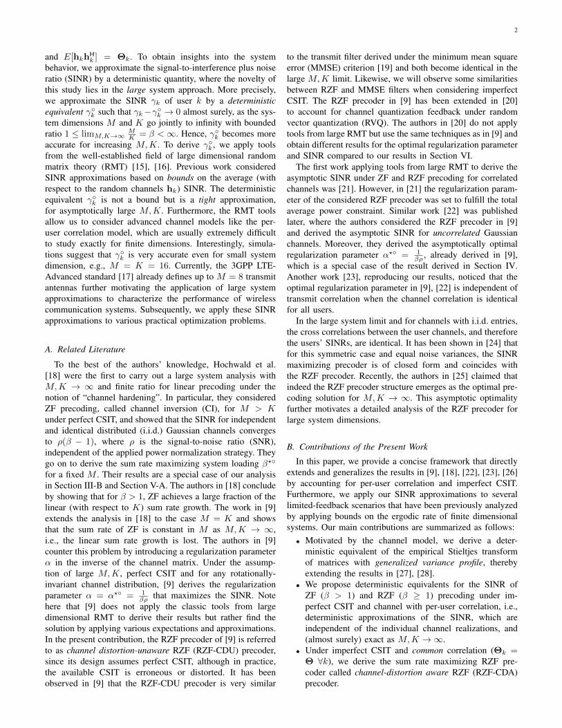


![Linear precoding design for massive MIMO based on the minimum mean square error algorithm · 2017. 8. 28. · (AMP) algorithm [11] and a successive over-relaxation (SOR)-based precoding](https://static.documents.pub/doc/80x56/60df5e6c9438bd6f591a2e5f/linear-precoding-design-for-massive-mimo-based-on-the-minimum-mean-square-error.jpg)


![[EURASIP 2013] Linear Precoding in Distributed MIMO Systems With Partial CSIT](https://static.documents.pub/doc/80x56/577cd2281a28ab9e78953348/eurasip-2013-linear-precoding-in-distributed-mimo-systems-with-partial-csit.jpg)


![MIMO Wireless Linear Precoding - Tufts Universitymaivu/papers/SPM_MIMO_Wireless_Precoding.pdf[Using CSIT to improve link performance] [Mai Vu and Arogyaswami Paulraj] MIMO Wireless](https://static.documents.pub/doc/80x56/5aaa561a7f8b9a95188df246/mimo-wireless-linear-precoding-tufts-maivupapersspmmimowirelessprecodingpdfusing.jpg)


