1

Last-Minute Bidding in Sequential Auctions with Unobserved,

Stochastic Entry

Ken Hendricks

University of Texas at Austin

Ilke Onur

University of New South Wales

Thomas Wiseman

University of Texas at Austin

September 2008

Abstract

We present a model of repeated, ascending price auctions for homogeneous goods

with unobserved, stochastic entry. Bidders have unit demands; they exit if they win, and

bid again if they lose. We show that, in equilibrium, entrants always bid in the next-to-

close auction and bidders always bid at the last minute. The more bidders present, the

lower is the continuation value of future auctions, so bidders avoid revealing themselves

until the end of the auction. Using a dataset of calculator auctions on eBay, we present

evidence that losers of an auction bid again in future auctions. Ordering the auctions by

closing time, we show that last-minute bidding is not merely the result of bidders going to

the next-to-close auction. Instead, bidding is concentrated at the end of the period in

which the auction is the next to close.

2

1. Introduction

In the United States, eBay has become the dominant player in the online auction

market, with sales of over $8 billion in 2007 (data from forbes.com). An important

feature of eBay is that auctions for identical products are held repeatedly, with many

auctions overlapping and closing one after another. For example, in our dataset of

auctions of Texas Instruments TI-83 Graphing Calculators, on average an auction closes

every 33 minutes, and the elapsed time between auctions is much smaller during peak

hours of the day when more users are actively bidding. The median time between

closings is 14 minutes. The availability of auctions that close at a later date allows

bidders who are outbid in one auction to bid again in another auction. Indeed, in our

dataset, most losers bid again. The objective of this paper is to explore how the option to

bid again conditional on losing can affect bids, the timing of bids, and prices in repeated

auctions of homogenous goods.

We study these issues using a simple model in which single units of a

homogeneous good are sold in an infinite sequence of continuous-time, ascending-price

auctions. Each auction lasts for one period, with a random number of new bidders

arriving each period. Buyers have unit demands. Because more than one bidder may

arrive during each period, there is also a stock of incumbent bidders waiting to obtain a

unit. Each bidder has the same valuation for a single unit of the good. Thus, bidders are

uncertain about the number of bidders but not about their valuations. Since losers bid

again, bidders use the outcomes of past auctions to determine their expectations of the

level of competition in the current and future auctions. We derive a symmetric

equilibrium in pure strategies in which entrants never delay but always reveal themselves

by bidding in the next-to-close auction. Entrants have an informational advantage over

incumbents and, as a result, each auction is won by an entrant if there is one and by an

incumbent otherwise. A key feature of the equilibrium is that an incumbent’s bid is set at

the level such that winning yields the same surplus as the expected surplus from waiting

until all the other incumbents are “cleared out” and then winning the next auction with no

competition. The incumbents’ bids (and prices) are thus increasing in the total number of

3

incumbents, so that entrants prefer to conceal their presence until the very end of the

auction, when it is too late for the incumbents to react.

The main conclusions of the analysis are that the option for losers to bid again

causes bidders to bid less than their true value and at the last minute. The markdown

factor depends upon the number of competitors that bidders expect to face in subsequent

auctions if they lose in the current auction. Entrants expect higher levels of competition

than incumbents since they know that they themselves are competitors. As a result,

entrants bid higher than incumbents and are more likely to win. This selection effect

arises from differences in information and not differences in valuations. The last-minute

bidding implies that bidders learn whether they are losers only at the end of an auction, at

which point, they bid again in a subsequent auction. Thus, as a first approximation, a set

of overlapping eBay auctions reduces to a sequence of second-price sealed bid auctions

ordered by their closing times.

Last-minute bidding (or “sniping”) in eBay auctions is well documented.

However, we introduce a new and informative approach of studying bid submission

times. Our dataset consists of every eBay auction of Texas Instruments TI-83 Graphing

Calculators held between June 15th, 2003 and July 30th, 2003. The comprehensive nature

of the dataset allows us to order these auctions consecutively according to their closing

times and focus on the intervals in which each auction is next to close. We then show that

last-minute bidding is not merely the result of bidders going to the next-to-close auction.

Instead, bidding is concentrated at the end of the interval in which the auction is the next

to close. The data also show that the assumption of unit demand is reasonable.

The organization of the rest of the paper is as follows. The next section describes

eBay and some related literature. We present the data in Section 3 and the model in

Section 4. Section 5 is the conclusion.

2. Background and Related Literature

EBay allocates items through auctions with proxy bidding, which is a mechanism

that bids on behalf of the bidder up to a maximum bid specified by him. At the end of the

4

auction, the bidder with the highest maximum bid wins the item at a price equal to the

second highest maximum bid submitted. The auction thus resembles an ascending

second-price auction. The seller sets the auction’s starting bid, which acts like a posted

reserve price since it is observed by all potential buyers. EBay also allows sellers to set a

secret reserve price that is not observable to the bidders. Potential buyers are informed

by eBay via email and a posting on the website whether the reserve price is met or not.

The seller selects the length of the auction: 1, 3, 5, 7 or 10 days.1 By choosing the

starting date and length of the auction, the seller determines the precise day and time that

it closes. There is no extension of auction length at the end of eBay auctions. This “hard-

close” rule gives bidders an opportunity to delay their bid submissions and place their

bids in the last minutes of the auctions. In a second-price setting with independent

private values, Vickrey (1961) shows that bidders have a weakly dominant strategy to bid

their valuations at any time during the auction. In practice, though, bidders on eBay tend

to wait until the very end of the auction to submit their maximum bids.

Most of the theoretical research on eBay auctions ignores the multi-auction

structure of eBay and focuses on the single unit auction. Roth and Ockenfels (2002) and

Ockenfels and Roth (2006) argue that late bidding could result from network congestion

that prevents some of submitted maximum bids from being recorded. When buyers all

submit maximum bids at the end of the auction, the resulting spike in network activity

decreases the probability that an individual maximum bid gets recorded. Under certain

conditions, buyers prefer to submit their maximum bids in the final seconds of the

auction, in the hope that competitors’ maximum bids will not be recorded. An earlier

submission would trigger all other buyers to submit their maximum bids early too. If the

potential gain from reduced competition outweighs the risk of not getting in a maximum

bid, then last-minute bidding is an equilibrium.

Bajari and Hortacsu (2003), Ockenfels and Roth (2006), and Rasmusen (2006)

show that last-minute bidding can arise in a single-unit auction if valuations have a

common component. In this environment, an early bid might reveal positive information

about the bidder’s estimate of the object’s value. That signal would cause other bidders

to bid more aggressively and raise the final price paid by the winner. One interpretation

1 While the data were collected, 1-day auctions were not an option for the sellers in eBay.

5

of our result is that the continuation value for losers introduces a common component to

the valuations of the bidders. Barbaro and Bracht (2005) suggest that last-minute bidding

is a best response to dishonest actions – “shill bidding” and “squeezing” – by the sellers

or sellers’ accomplices. A shill bid is a high maximum bid that a seller submits in her

own auction under a false name. She thus can learn the value of the highest legitimate

maximum bid. Then the seller cancels the shill bid and replaces it with another just

below the highest legitimate maximum bid. In that way, any potential gain for the buyer

is squeezed from him by the seller. Waiting until the very end of the auction to submit a

maximum bid is a way to prevent shill bidding.

The main difficulty in studying eBay auctions as a sequence of single unit

auctions is that losing bids are observable. Since rivals can exploit this information in

subsequent auctions, bidders have an incentive to “hide” their types, which often leads to

non-existence of equilibria in monotone bid strategies. (See Milgrom and Weber (2000).)

Wang (2006) gets around the problem by focusing on a model with only two goods. In

the second auction, bidding one’s valuation is a weakly dominant strategy, and so

information about opponents’ type does not affect bidding strategies. He shows that last-

minute bidding in the first auction is the outcome of the unique symmetric sequential

equilibrium in undominated, monotone strategies. Zeithammer (2006) studies an infinite-

horizon model of sealed-bid, private-value auctions when future auctions arrive

randomly. His model is similar to ours in several respects, but he assumes that bidders

have no memory and therefore cannot learn from outcomes of past auctions. He does

provide evidence that bidders lower their bids in response to higher arrival rates of close

substitutes.2

Empirical studies of bidding in eBay auctions that take a structural approach also

focus on the single-unit auction. Lewis (2007) and Bajari and Hortascu (2003) argue that

the prevalence of late bidding justifies modeling eBay auctions as a second-price sealed-

bid, common-value auction. Gonzalez, Hasker, and Sickles (2004), Canals-Cerda and

Pearcy (2006), and Ackerberg, Hirano, and Shahriar (2006) adopt the independent private

2 Other papers looking at sequential auctions include Ashenfelter (1989), Gale and Hausch (1994), Jeitschko (1999), Katzman (1999), McAfee and Vincent (1993), Milgrom and Weber (2000), and Pitchik and Schotter (1988). These papers either study the two-good case in which bidders have a dominant strategy in the second auction or assume that losing bids are not observable.

6

values model.3 The first study assumes that entry is exogenous and that the number of

potential bidders is constant across auctions. The latter two studies assume that the

number of bidders is the stochastic outcome of a Poisson process. Bidders are assumed

to bid upon arrival if their valuations exceed the standing high bid.4 The sale price in all

three studies is determined by the second-highest valuation among the set of potential

bidders, which plays a key role in identifying the underlying distribution of valuations.

Consequently, all three studies assume that the bidder’s continuation value conditional on

losing is zero or, more generally, a constant that does not depend upon the level of

competition (and therefore on auction outcomes). Our results suggest that this

assumption is quite strong and unlikely to hold in thin markets.

3. Data and Analysis

In this section we establish three stylized facts that motivate our modeling

assumptions: last-minute bidding occurs, buyers have unit demand, and losers in an

auction bid again in future auctions with positive probability. We also demonstrate three

features consistent with the predictions of our model: new entrants are both more likely to

bid at the last minute and more likely to win the auction than incumbents, and item prices

increase with the number of losing bidders from recent previous auctions.

Data

Our dataset consists of information collected on Texas Instruments TI-83

Graphing Calculator auctions featured on eBay. The advantages of studying the TI-83

are a high volume of auctions and the relatively homogeneous nature of the product. The

data cover every auction between June 15th, 2003 and July 30th, 2003. Private auctions,

in which information about the bidders is not available, and so-called “Dutch auctions” of

multiple units are excluded from our dataset. We also exclude “Buy-It-Now” auctions, in

3 Interestingly, Canals-Cerda and Pearcy find that, in their dataset of paintings, last-minute bidding is not nearly as prevalent as in other datasets. The reason may be that the paintings are heterogenous, so that losers are less likely to bid against each other in subsequent auctions. 4 However, they do not assume that bidders bid their valuations upon arrival, so that they can account for bidders that bid multiple times in an auction.

7

which a buyer can pre-empt the auction by paying a posted price selected by the seller.5

During the time that our data were collected, eBay’s website did not reveal whether or

not an auction ended in a transaction. We assume that all auctions that attracted a bid

ended with a sale, and that the winner was the buyer with the highest standing bid.

The sale prices for TI-83 calculators in retail stores in the summer of 2003 were

between 80 and 100 dollars for new items and between 40 and 60 dollars for used ones.

The final prices of the auctions we have in our dataset differ substantially – some items

are new, some are used, and some come with additions like cases or operating manuals.

However, our dataset also contains auctions offering these additions without the

calculator, or more than one calculator bundled together. In order to be more consistent

with the items being offered in our dataset we keep only the auctions that have a

transaction price between 20 dollars and 110 dollars.

There are 1,817 unique auctions completed in the 6-week period. We observe

4,404 bidders who submit a total of 13,240 maximum bids.6 Moreover, we observe 192

unique auctions that did not receive any bids or were cancelled. We exclude those

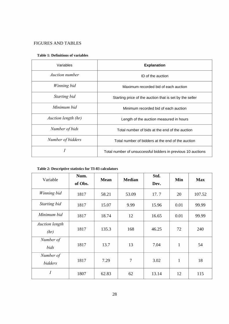
auctions. We collect the following information for each TI-83 auction: auction number,

starting bid, number of bids, auction length, winning bid, minimum bid and number of

bidders. Table 1 presents a brief description of these variables, and Table 2 provides

descriptive statistics. The winning bid is the price that the winner pays at the end of the

auction. This price is the maximum bid of the second-highest bidder plus the bid

increment. The calculators sell for a bit more than $58 on average, with a standard

deviation around $17. The average starting bid set by the seller is just above $15, and the

lowest submitted bid is a little below $19 on average. The average auction lasts 5.5 days

and attracts 14 bids. The average number of bidders is 7, with standard deviation equal to

3. We note that the ratio of standard deviation to mean is significantly higher for the

number of bidders than for the sale price, a difference consistent with our assumption that

there is more uncertainty about the number of bidders than about their willingness to pay.

5 The Buy-It-Now option in such an auction disappears as soon as a maximum bid above the reserve price is submitted, and the auction becomes indistinguishable from one that never had the Buy-It-Now option. Therefore, our dataset likely includes some wiped-out Buy-It-Now auctions. 6 We detected 229 bids without any bidder ID. Fortunately, most of these bids do not affect the outcomes of the particular auctions.

8

We also use a subset of our data to follow the behavior of individual bidders. We

choose a 4-day window, July 5 through July 8, 2003, in the middle of the dataset and

identify all the bidders active in that window. We then track their outcomes forward and

backward in time. By choosing a window in the middle of the range of dates, we can

avoid truncation problems and observe bidders’ entire histories. The window, consisting

of a Saturday through a Tuesday, includes both weekends and weekdays, in order to

capture any day-effects. We use this subset to study how buyers react after winning or

losing an auction. There are 720 unique bidders who submit at least one maximum bid in

the 4-day period. In total, those bidders submit 8,186 bids over the entire six-week

sample.

Analysis

First we look at last-minute bidding. We introduce a new and informative

approach of studying bid submission times. Many auctions on eBay have ending times

that are fairly close together. If buyers submit their bids in whichever auction ends next,

then that closeness may generate the appearance of last-minute bidding without any

strategic intent by buyers to delay their bids. For example, if each auction ends one

minute after the previous auction, and bidders participate only in the next auction to

close, then all bidding will be in the last minute. To distinguish that effect from true last-

minute bidding (where buyers wait until competitors can no longer respond), we arrange

the auctions sequentially by their closing times and look at bidding behavior during the

interval when an auction is the next to close. We find evidence of both sorts of bidding.

A search for “TI-83 calculator” on eBay yields a list of auctions sorted by closing

time, with the next auction to close listed at the top. There is thus a natural tendency for

buyers to participate in soonest-ending auction. To see how close together auctions end,

we define for each auction in our sample the closing interval. The closing interval of an

auction is the time period during which that auction is the next to close; that is, the time

from when the previous auction closes to when the current auction closes. In Tables 3

and 4 we present descriptive statistics on the lengths of the closing intervals. On average,

the closing times for auctions are 33 minutes apart, with a minimum of 0 (that is, less

than one minute) and a maximum of almost 12 hours. The median length of a closing

9

interval is 14 minutes. Many of the auctions in our dataset close soon after the previous

one ends. For more than 6 percent of the auctions, the closing interval is less than one

minute long. Moreover, almost one third of the auctions have 5 minutes or less between

their closing times.

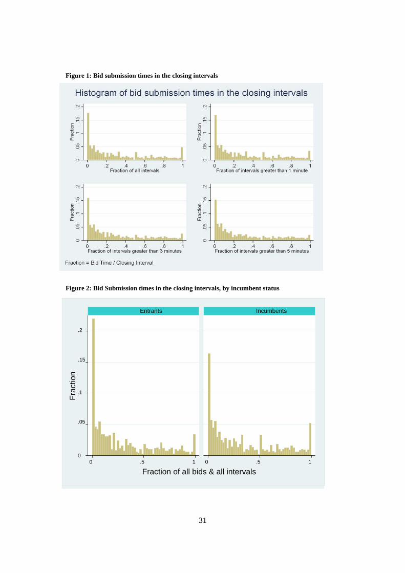
The prevalence of very short closing intervals may create misleading measures of

last-minute bidding. In response, we examine the distribution of bid times relative to the

length of the closing interval. The histograms in Figure 1 show the submission times of

maximum bids, measured as the fraction of the auction’s closing interval remaining. For

example, if an auction’s closing interval is two minutes long, then a bid submitted 30

seconds before the end is recorded as being submitted at time 0.25. In auction with a 20-

minute closing interval, time 0.25 corresponds to 5 minutes from the end. Each bin in the

histograms represents 2 percent of the length of the closing interval. The first histogram

includes all the auctions in our dataset. Subsequent histograms exclude auctions with

closing intervals below 1, 3, and 5 minutes, respectively.

The histograms show a spike at time 1, just when the previous auction ends.

Overall, 5 percent of bids are submitted before 2 percent of the closing interval has

elapsed. (The first 2 percent of the median 14-minute closing interval is the first 17

seconds.) That spike becomes smaller, though, in the other histograms, as we look at

auctions with longer closing intervals. The histograms also show a larger spike in the

first bin, the last 2 percent of the closing interval. In all four cases between 20 and 25

percent of maximum bids are submitted after 98 percent of the closing interval has

elapsed. Thus, although some late bidding seems to be driven merely from buyers

arriving in the soonest-ending auctions, we also find evidence that some buyers wait until

the very end of auctions to participate: last-minute bidding is not an illusion resulting

from closely-spaced auctions.

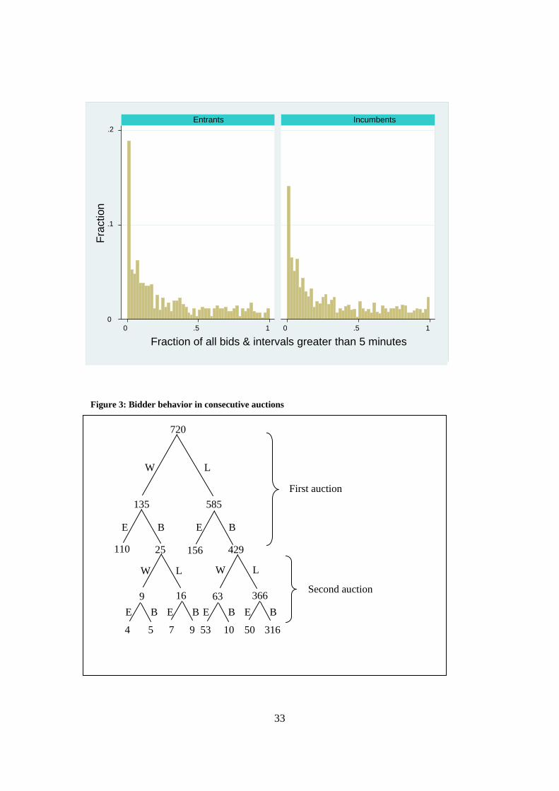
Figure 2 breaks down the histograms of Figure 1 according to whether or not the

bidder has participated in an earlier auction in the dataset. In all four cases, entrants are

more likely to submit a maximum bid in the last 2 percent of the closing interval than are

incumbents. Entrants are also less likely to submit a maximum bid during the first 2

percent of the interval.

10

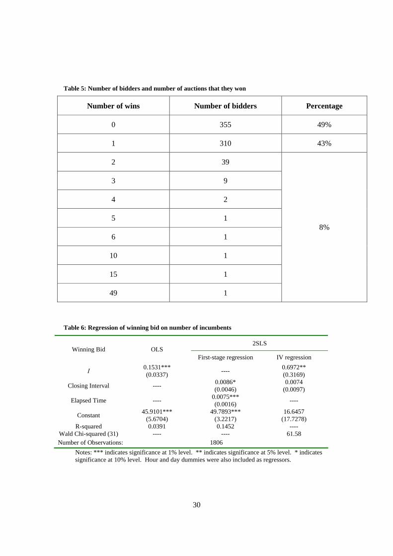
Next, we look at the decisions made by bidders after winning or losing an auction.

Table 5 breaks down the 720 buyers in the sub-sample according to how many auctions

they win in the entire six-week period. The table shows that 365 of the bidders win at

least one auction, and together those 365 win 508 auctions. Among the 365 winners, 310

(85 percent) win a single auction. It appears, then, that the assumption of unit demand is

reasonable for most bidders.

We also track the 720 bidders from the first auction that they participate in.

Figure 3 shows that 135 of the 720 win (W) their first auction. Of those initial winners, a

large fraction (110/135) exit (E) eBay’s website – the dataset contains no future bids for

them. Of the 585 bidders who lose (L) their first auction, most (429) bid (B) in at least

one subsequent auction. Of those 429, 366 lose their second auction, and 316 of those

366 bid again. Of the 63 who win on their second try, 53 exit. We conclude that, to a

first approximation, buyers have unit demands, and losers of an auction try again in

subsequent auctions. We also note that entrants (participating in their first auction) win

22% more frequently than incumbents - 135/720 vs. 63/429.

Finally, to explore how the presence of incumbents affects bidding behavior, for

each auction in our sample (except the first ten) we construct a variable I, equal to the

number of bidders who submitted a maximum bid in at least one of the previous ten

auctions, but who did not win an item. The mean number of such incumbents is 62.8.

We regress winning bids on I (plus day-of-the-week and time-of-day dummies). Out of

concern that the number of incumbents I may be endogenous (if the entry rates of buyers

are correlated across time, then I will be correlated with the expected number of new

bidders), we instrument for I using the length of the closing interval and the elapsed time

of the past ten auctions.7 The results are presented in Table 6. Two-stage least-squares

regression yields a positive and statistically significant coefficient: the coefficient is

0.697, with a standard error of 0.317. That is, an additional incumbent increases the

expected price in an auction by $0.70, or 1.2% of the mean price. A log specification

7 To be precise, we define the elapsed time variable for auction n as the time from when auction n – 11 closes to when auction n – 1 closes. Elapsed time is likely to be positively correlated with the number of losing bidders since more bidders arrive when the time interval covered by the ten auctions is longer. If the arrival rate of sellers is more or less exogenous, though, elapsed time is likely to be uncorrelated with the number of entrants in the current auction.

11

yields very similar results. We conclude that auction prices are higher when the stock of

bidders who lost recent auctions is greater.

4. Model

We study the following simplified version of the eBay auction setting.

Environment

There is an infinite sequence of auctions, each of a single unit of a homogeneous

good. All buyers are risk-neutral, their utility is quasilinear in wealth, and they discount

the future at a rate δ ∈ (0, 1) per period. In each period, a maximum of two new buyers

enter. Each entry occurs with independent probability p. A buyer exits only after he has

obtained a unit of the good. We discuss the implications of this assumption and the

consequences of relaxing it in the next section. Each buyer wants one unit of the good,

and values that one unit at V > 0. All buyers are expected-utility maximizers. The

structure is common knowledge, although a buyer’s arrival is not observed by other

buyers until he participates in an auction.

Auctions are held consecutively, one per period. Within each period, an auction

is a continuous-time, first-price auction with proxy bidding (described below). Auction t

runs from time t to time t + 1, for t ∈ {1, 2, …}. The assumption that the auctions do not

overlap is not important. What matters is that they have different ending times.8 The

(publicly observed) reserve price in each auction is the same and is normalized to zero.9

The auctions use a proxy-bidding program. A buyer who chooses to participate

enters a “maximum bid” b, and the program bids on his behalf up to that level. If b

exceeds h, the previous high maximum bid, then the program automatically enters a bid

of h plus a small, discrete increment ε. We assume that the minimum bid increment ε is

8 In the equilibrium that we construct, each active bidder participates in each auction. Papers looking at selection of buyers across different sellers include Bajari and Hortascu (2003), Dholakia and Soltysinski (2001), McAfee (1993), Peters and Severinov (2006), and Stryszowska (2004). 9 Actual eBay auctions have both a public “starting bid” and a hidden “reserve price,” as described in Section 2.

12

vanishingly small. In particular, we assume that a buyer is indifferent between paying r

for the good and paying r + ε, as long as r < V, but is unwilling to pay V + ε. If two or

more buyers enter the same maximum bid b > h at the same time, then the tie is broken

randomly with equal probabilities: the program records a bid of b for one of the buyers

and b − ε for the other(s). If a buyer with maximum bid b has the current high bid h, and

another buyer enters a maximum bid b′ between h and b, then the program automatically

enters a new bid of b′ for the first buyer and a bid of b ε′ − for the second. Having

entered a maximum bid, a buyer can neither retract it nor revise it downward, although he

can increase it at any time before the end of the auction. When the auction ends, the item

is awarded to the buyer with the highest bid at a price equal to his bid. That outcome is

publicly observed.

Throughout, we distinguish between a buyer’s maximum bid (the price that he

gives the program) and his bid (which the program makes on his behalf as a function of

the maximum bids of all bidders, and the order in which they were entered). Bids are

publicly observed, but maximum bids are private information (except to the extent that

they are revealed by bids). Thus, the auction is first-price in bids, but it resembles a

second-price auction in maximum bids.

Each buyer observes the history of bids and outcomes in all auctions so far. Thus,

if new entrants always submit a maximum bid in the first available auction, then the

number of incumbent buyers (those who have bid in previous auctions but have not yet

won an item) is common knowledge.

A pure strategy for a buyer tells him whether and at what amount to enter a

maximum bid, as a function of time, the observed history, and his own previous actions.

A buyer cannot enter a maximum bid in an auction before that auction begins, or take any

action before he himself enters. Mixed strategies are defined straightforwardly.

Outcomes

We construct a symmetric, sequential equilibrium in pure strategies. In particular,

in equilibrium a buyer entering in period t submits a maximum bid at the end of auction t,

so that the number of incumbent buyers is common knowledge. After entering, a buyer

13

participates in every auction until he wins an item. (We note that this feature of the

equilibrium is a simplification relative to the pattern observed in the data. Although, as

demonstrated in the previous section, losing bidders in our dataset usually participate

again in subsequent auctions, they typically do not bid in the next auction to close.) As a

preliminary, we define the function S(n), n ∈ {1, 2, … }, recursively as

(1)1

aS Vcd

=−

and )1()( 1SdnS n−= , where

2(1 )

1 2 (1 )pa

p pδδ

−=

− −,

2

1 2 (1 )pcp p

δδ

=− −

, and c

acd2

411 −−= .

In the equilibrium to be constructed, S(n) will be the expected (undiscounted) surplus for

an incumbent at the beginning (i.e., before the number of new entrants is known) of a

period in which the total number of incumbents is n. We also define the maximum

bidding functions bi(n) and be(n) for incumbents and entrants, respectively:

(1) 0ib = , ( ) ( 1)ib n V S nδ= − − for n ≥ 2, and )2()( += nbnb ie .

A buyer who obtains an item at price bi(n) gets surplus δS(n – 1). With that notation, we

can state our results. Proposition 1 describes the equilibrium.

Proposition 1: For any auction t, let nt be the number of buyers who i) have submitted a

maximum bid in a previous auction, and ii) have not yet obtained an item. Let jt be the

number of buyers who i) submit a maximum bid before the end of auction t, and ii) have

not entered a maximum bid in a previous auction. Then the following strategies and

beliefs for each auction t constitute a sequential equilibrium:

At the end of auction t, at time t + 1, an incumbent submits a maximum bid of

( )it tb n j+ if he has previously submitted a maximum bid, and a maximum bid of

( 1)et tb n j+ + otherwise.

14

An entrant waits until the end of the auction to submit a maximum bid. He

submits a maximum bid of ( )et tb n j+ , unless he himself is one of the jt early bidders, in

which case he submits a maximum bid of ( 1)it tb n j+ − .

Beliefs (about the number of buyers) at histories reachable in equilibrium are

given by Bayes’ rule. Off-equilibrium, a buyer is believed to be present from the time

that he submits a maximum bid until he wins an item. (A history in which a buyer who

was supposed to submit a maximum bid has not yet done so is indistinguishable from a

history in which that buyer did not arrive, and thus in on the equilibrium path.)

In equilibrium, nt will equal the number incumbents, and jt will always be zero,

since time-t entrants reveal their types at the end of auction t. Each auction is won by an

entrant, if there is one. Conditional on there being no entrant, an incumbent is indifferent

between winning at a price equal to his maximum bid ( )itb n or waiting until the next

auction, in which there will be one fewer incumbent. The expected surplus S(nt), then,

can be interpreted as the expected payoff that the incumbent would get from by waiting

until the first auction in which i) there are no other incumbents left, and ii) no new buyers

enter; and then winning that auction, uncontested, for price zero (+ ε). As the number of

incumbents n rises, the expected wait until that first uncontested auction increases, and

the expected discounted surplus falls. Thus, S(n) is decreasing (exponentially) in n.

Note that the value of the parameter d is strictly between 0 and 1, and that its limit

as the discount factor δ approaches 1 is 1. The same is true of the expression a/(1 – cd).

For any fixed number of incumbents n, as buyers become more patient, the expected

discounting of the time before the first uncontested auction becomes negligible, and the

expected surplus S(n) approaches V. That is,

1lim ( )S n Vδ→

= for n ∈ {1, 2, … }.

For any fixed discount rate δ less than 1, lim ( ) 0n S n→∞ = . Thus, in thick markets, bids

are very close to V.

15

An entrant’s maximum bid be(n) is set at the price that makes him indifferent, if

there is a second entrant, between winning at that price and proceeding to the next

auction, in which there will be n + 1 incumbents, including himself. If there is a single

entrant, then he wins the auction at a price of bi(n). That outcome yields him surplus

δS(n – 1), which is strictly greater than δS(n), the surplus that he would expect from

losing the auction and proceeding to the next, where there will be a total of n incumbents

(himself, plus the n previous incumbents, minus the winner). That is, in equilibrium a

single entrant has an advantage, in the sense that his surplus from winning the first

auction strictly exceeds the expected continuation payoff. One way to interpret this

advantage is as the payoff to being better informed than the incumbents about the number

of buyers – an entrant, knowing that there are at least n + 1 buyers, expects a lower

continuation value than the incumbents and thus is willing to submit a higher maximum

bid.

In principle, a period-t entrant need not submit a maximum bid in auction t. In

that case, he would be a “hidden” incumbent in the next auction, and so would have an

informational advantage. The other buyers would underbid (since both maximum

bidding functions be(n) and bi(n) are strictly increasing in n), and the hider could win the

auction at a below-equilibrium price. However, as will be shown in the proof of

Proposition 1 below, that advantage is outweighed in expectation by the advantage

provided in equilibrium to a lone entrant. Thus, all entrants reveal themselves; that

revelation simplifies the structure of the equilibrium considerably.

Proof of Proposition 1: First, we show that if the proposed equilibrium strategies are

followed, then the expected surplus to an incumbent, given nt, at time t is given by the

function S(nt), as claimed. Suppose that there is a single incumbent at the beginning of

an auction; that is, n = 1. With probability

20 (1 )p p≡ − ,

16

there are no entrants, and he wins the auction at price zero. If there is a single entrant,

then the incumbent loses the auction and continues to the next auction, in which n is still

1. That event has probability

1 2 (1 )p p p≡ − .

Finally, if there are two entrants (probability

212 4 (1 )p q≡ − ),

then the incumbent loses the auction, as does one of the entrants, and in the next auction

n increases to 2. Letting f(2) be the expected continuation payoff in an auction with 2

incumbents, the incumbent’s expected payoff at the start of the auction is thus given by

0 1 2(1) (1) (2)f p V p f p fδ δ= + + .

Solving for f(1) yields

0 2

1 1(1) (2)

1 1p pf V f

p pδ δδ δ

= +− −

. (1)

Similarly, we can calculate the expected payoff f(n) when there are n incumbents at the

beginning of the auction. If there are no entrants, then one of the n incumbent high types

wins at price ( ) ( 1)ib n V S nδ= − − , and the others proceed to the next auction, when the

number of incumbents will be n – 1. If there is one entrant, then the entrant wins, and

there are still n incumbents in the next auction. If there are two entrants, then one of

them wins, and the next auction has n + 1 incumbents. The expected payoff to an

incumbent, then, is given by

17

( )110 1 2( ) ( 1) ( 1) ( ) ( 1)n

n nf n p S n f n p f n p f nδ δ δ δ−= − + − + + + .

Solving for f(n) yields

( )0 11 2

1 1( ) ( 1) ( 1) ( 1)

1 1n

n np pf n S n f n f n

p pδ δδ δδ δ

−= − + − + +− −

. (2)

Combining Expressions 1 and 2 gives a second-order difference equation whose solution

is f(n) = S(n) for n ∈ {1, 2, … }, which was to be shown. Note that the function S(n)

satisfies the following condition:

0 1 2( ) ( 1) ( ) ( 1)S n p S n p S n p S nδ δ δ= − + + + , (3)

where for the sake of convenience S(0) is defined as Vδ

.

Next, we show that the proposed strategies are best responses. First, consider an

incumbent who has already revealed his presence, and let the total number of incumbents

(including those who have submitted a maximum bid for the first time during the course

of the current auction) n ≥ 1 be given. Such a buyer is indifferent over when to submit

his maximum bid, since his presence is already known, and thus is willing to submit at

the end of the auction.10 Submitting any maximum bid up to be(n) (or submitting no

maximum bid) in the current auction yields the same expected continuation payoff, S(n).

A maximum bid above be(n) wins the auction for sure, at price be(n) if there is at least one

entrant and at price bi(n) otherwise, yielding

( )0 1 2( 1) ( 1)p S n p p S nδ δ− + + + . (4)

10 Introducing a small probability that incumbents exit exogenously between auctions would make incumbents strictly prefer to bid at the last minute, as we discuss in the next section.

18

Since ( )S ⋅ is decreasing, the value of Expression 4 is less than the value of Expression 3.

Finally, by submitting a maximum bid equal to be(n) the incumbent wins the auction at

price bi(n) if no new buyers enter. If m {1,2}∈ buyers enter, then the incumbent wins at

price be(n) with probability 11m+

, and otherwise proceeds to the next auction with

1n m+ − other high-type incumbents. Thus, a maximum bid of be(n) yields

( )1 10 1 22 2( 1) ( ) ( 1) ( 1)p S n p S n S n p S nδ δ δ δ− + + + + + ,

which similarly is less than Expression 3.

Second, consider an entrant when there are n ≥ 1 high-type incumbents. Since

submitting a maximum bid before the end of the auction causes other buyers to raise their

maximum bids, he prefers to submit at the last minute, if he submits a maximum bid at

all. If he does submit a maximum bid in auction t, he cannot do better than submitting

be(n). Call ( )eS n the expected payoff from submitting be(n) (or any higher maximum

bid), where

( ) (1 ) ( 1) ( 1)eS n p S n p S nδ δ= − − + + . (5)

If a second buyer enters (probability p), the entrant gets surplus ( 1)S nδ + either from

winning the current auction at price be(n) or proceeding to the next auction with n other

incumbents. If there is no second entrant (probability 1 p− ), the entrant wins the auction

at price bi(n). Submitting a maximum bid strictly between bi(n) and be(n) yields the same

payoff, ( )eS n . A maximum bid less than bi(n) means proceeding to the next auction, and

thus yields

(1 ) ( ) ( 1)p S n p S nδ δ− + + ,

which is less than Expression 5. A maximum bid of exactly bi(n) yields

19

( )11 1(1 ) ( 1) ( ) ( 1)n

n np S n S n p S nδ δ δ+ +

− − + + + ,

which is also less than ( )eS n . When n = 0, be(0) is an optimal maximum bid, since the

payoff from submitting any positive maximum bid is

(0) (1 ) (1)eS p V p Sδ= − + .

Thus, an entrant’s choice is between entering a maximum bid of be(n) or “hiding”

by submitting no maximum bid. Let ( )hS n denote the expected continuation payoff to a

“hidden” incumbent (that is, one who arrived in a previous auction but did not reveal his

presence) from submitting the equilibrium maximum bid be(n + 1), with the number of

other incumbents n given. (We show below that that maximum bid is optimal.) That

maximum bid ensures that the hidden incumbent will win the auction, at price be(n) if

there is at least one entrant and at price bi(n) otherwise. Thus, the value of ( )hS n is

given by

( )

( )0 1 2

0 1 2

(0) (1), and

( ) ( 1) ( 1) for 1.

h

h

S p V p p S

S n p S n p p S n n

δ

δ δ

= + +

= − + + + ≥ (6)

We claim that for any tn , ( )eS n is greater than 1( ) |ht tE S n n+⎡ ⎤

⎣ ⎦ , and so therefore an

entrant’s best response is to enter a maximum bid of be(n) rather than to “hide.” (The

proof of Lemma 1 is in the appendix.)

Lemma 1: 1( ) ( ) | for all 0.e ht t tS n E S n n n+⎡ ⎤> ≥⎣ ⎦

20

All that remains is to demonstrate that submitting a maximum bid of be(n + 1) is optimal

for a “hidden” incumbent when there are n other incumbents. First, we show that if he

submits a maximum bid at all, be(n + 1) is optimal. (As with an entrant, he prefers to

submit at the end of the auction.) Submitting any maximum bid strictly higher than be(n)

yields expected continuation payoff ( )hS n , as defined in Expression 6. Suppose that n ≥

1. Then submitting a maximum bid of be(n) yields

( )1 20 1 2 3 3( 1) ( 1) ( 1) ( 2) ,p S n p S n p S n S nδ δ δ δ− + + + + + +

and a maximum bid strictly between bi(n) and be(n) yields

0 1 2( 1) ( 1) ( 2).p S n p S n p S nδ δ δ− + + + +

Since ( )S ⋅ is decreasing, both values are less than ( )hS n . A maximum bid of bi(n)

yields

( )1 10 1 21 1( 1) ( ) ( 1) ( 2),n np S n S n p S n p S nδ δ δ δ

+ +− + + + + +

and any maximum bid below bi(n) yields S(n + 1); both values are less than ( )hS n .

Thus, be(n + 1) is an optimal proxy bid.

If n = 0, the argument is similar. Any maximum bid higher than be(n) yields

(0)hS . Maximum bids equal to be(n) and below be(n) yield, respectively,

( )1 20 1 2 3 3( ) (1) (1) (2)Hp V R p S p S Sδ δ δ− + + + and

0 1 2( ) (1) (2),Hp V R p S p Sδ δ− + +

21

both of which are below (0)hS .

To see that a hidden incumbent expects to do better by submitting a maximum bid

of be(n + 1) than by waiting, recall that the proof of Lemma 1 shows that

1( ) ( ) | for all 0.h ht t tS n E S n n nδ +

⎡ ⎤≥ ≥⎣ ⎦

The law of iterated expectations, together with the fact that a hidden incumbent must

eventually submit a maximum bid in some auction to make any surplus, then implies that

submitting a maximum bid of be(n + 1) is optimal. Q.E.D.

5. Concluding Remarks

We have presented a model of sequential auctions of identical goods with

stochastic entry in which losing bidders bid again. The equilibrium is fully revealing:

entrants reveal their presence in the same period that they arrive. In general, full

revelation is difficult to obtain in sequential auctions because of the information leakage

problem. A bidder may be reluctant to submit a high bid in auction t, because if he loses

his competitors will deduce that he has a high valuation and thus bid more aggressively in

auction t + 1. Our infinite-horizon model focuses on bidders learning about the number

of rivals rather than about their valuations. In equilibrium, the bidding advantage given

to an entrant outweighs the future benefit from convincing competitors that he is absent,

and thus he is willing to reveal himself.

The equilibrium has several features of empirical interest. First, bids depend upon

the state of competition. When the number of buyers is high, the chances of winning a

unit at favorable prices fall, and bidders bid more aggressively. This result may seem

obvious, but in many of the theoretical and empirical models of eBay auctions, bidders

are assumed to bid their value independently of the number of rivals. Second, entrants in

an auction are more likely to win than incumbents. This selection effect arises from the

fact that the entrant is better informed than incumbents about the number of competitors,

22

and not because of differences in valuations. Third, entrants bid at the last minute. The

last-minute bidding is driven by two factors: uncertainty about the number of bidders

present and the possibility that losing bidders will compete again in future auctions.

Because the presence of an additional competitor reduces the expected surplus from

waiting until the next auction, incumbent bidders bid more aggressively if they know an

entrant has arrived. Therefore, entrants wait until the end of an auction, when it is too

late for other bidders to react, to reveal themselves by submitting a maximum bid.

Incumbents bid in every auction until they win and they are indifferent as when to

bid during an auction. These results follow from the assumption that bidders do not exit

except by winning. If we introduced a probability of exogenous exit, then incumbents

would have private information about their participation in much the same way that

entrants have. The private information would give incumbents an incentive not to reveal

themselves until the last minute. In fact, incumbents would have an incentive to pretend

to exit, lowering their rivals’ expectations of the number of bidders and bids in

subsequent auctions, and then bid in the next auction.

We conjecture that if we add a very small probability of exit, then the new

equilibrium will involve a very small probability of an incumbent hiding in each auction

conditional on not exiting. In other words, incumbents play a mixed strategy in which

they are indifferent between bidding at the last minute in the current auction and waiting

until the next auction to bid. The intuition is that the rivals’ belief that an incumbent has

exited after not bidding would have to very low in order to balance the gain from hiding

(in the form of slightly lower competitors’ bids in the future) and the cost of missing a

chance to win the product for a low price in the current auction (if other incumbents

choose to hide).11 So our equilibrium may be robust in the following sense: if there is 1

percent chance of exit, then incumbents bid with 99 percent probability instead of 100

and are certain to bid at the last minute. Confirming this conjecture is beyond the scope

of this paper.12 More generally, allowing bidders to exit would be an interesting

extension of our model.

11 This kind of “low probability of behavioral type implies low probability of mimicking” result is standard in reputation models. See, for example, Mailath and Samuelson’s (2006) chapter 17. 12 One technical complication is that the tractable second-order difference equation in Expressions 1 and 2 would become of order n + 2: each of two entrants might arrive, and each of n incumbents might exit.

23

As Roth and Ockenfels (2002) show, last-minute bidding behavior is sensitive to

the details of auction closing rules. In our model, as in Roth and Ockenfels, last-minute

bidding depends on the hard closing rule. With a soft close (meaning that the auction is

extended whenever a maximum bid is submitted near the closing time), rivals always

have a chance to respond to the information revealed by a late bid, and entrants cannot

effectively conceal themselves. Another interesting topic for future research is to try to

extend our model to correspond to the rules of other online auction sites, such as

Amazon.com or ubid.com.

24

References

Ackerberg, D., Hirano, K., and Shahriar, Q. (2006). “The Buy-it-Now Option, Risk Aversion, and Impatience in an Empirical Model of eBay Bidding,” working paper.

Ashenfelter, O. (1989). “How Auctions Work for Wine and Art,” Journal of Economic

Persepectives, 3, pp. 23-36. Bajari, P. and Hortacsu, A. (2003). “The Winner's Curse, Reserve Prices and

Endogenous Entry: Empirical Insights from eBay Auctions”, RAND Journal of Economics, 34, pp. 329-355.

Barbaro, S. and Bracht, B. (2006). “Shilling, Squeezing, Sniping: Explaining late

bidding in online second-price auctions,” working paper. Canals-Cera, J.J. and Pearcy, J. (2006). “Econometric Analysis of English Auctions:

Applications to Art Auctions on eBay,” working paper. Dholakia, U. and Soltysinski, K. (2001). “Coveted or Overlooked? The Psychology of

Bidding for Comparable Listings in Digital Auctions,” Marketing Letters, 12, pp. 225-237.

Gale, I. and Hausch, D. (1994). “Bottom-fishing and declining prices in sequential

auctions,” Games and Economic Behavior, 7, pp. 318-331. Gonzalez, R., Hasker, K., and Sickles, R. (2004). “An Analysis of Strategic Behavior in

eBay Auctions,” working paper. . Jeitschko, T. (1999). “Equilibrium Price Paths in Sequential Auctions with Stochastic

Supply,” Economics Letters, 64, pp. 67-72. Katzman, B. (1999). “A Two Stage Sequential Auction with Multi-Unit Demands,”

Journal of Economic Theory, 86, pp. 77-99. Lewis, G. (2007). “Asymmetric Information, Adverse Selection and Seller Disclosure:

The Case of eBay Motors,” working paper. Mailath, G. and Samuelson, L. (2006). Repeated Games and Reputations: Long-run

Relationships. Oxford: Oxford University Press. McAfee, R. (1993). “Mechanism Design by Competing Sellers,” Econometrica, 61, pp.

1281-1312.

25

McAfee, R. and Vincent, D. (1993). “The Declining Price Anomaly,” Journal of Economic Theory, 60, pp. 191-212.

Milgrom, P. and Weber, R. (2000). “A Theory of Auctions and Competitive Bidding II,”

in P. Klemperer (ed.), The Economic Theory of Auctions, Cheltenham, U.K.: Edward Elgar.

Ockenfels, A. and Roth, A. (2006). “Late and multiple bidding in second price Internet

auctions: Theory and evidence concerning different rules for ending an auction,” Games and Economic Behavior, 55, pp. 297-320.

Peters, M. and Severinov, S. (2006). “Internet Auctions with Many Traders,” Journal of

Economic Theory, 130, pp. 220-45. Pitchik, C. and Schotter, A. (1988). “Perfect Equilibria in Budget-Constrained Sequential

Auctions: An Experimental Study,” RAND Journal of Economics, 19, pp. 363-388.

Rasmusen, E. (2006). “Strategic Implications of Uncertainty over One's Own Private

Value in Auctions,” B.E. Journals in Theoretical Economics: Advances in Theoretical Economics, 6, pp. 1-24.

Roth, A. and Ockenfels, A. (2002). “Last-Minute Bidding and the Rules for Ending

Second- Price Auctions: Evidence from eBay and Amazon Auctions on the Internet,” American Economic Review, 92, pp. 1093-1103.

Stryszowska, M. (2004). “Late and Multiple Bidding in Competing Second Price

Internet Auctions,” FEEM Working Paper No. 16.2004. Vickrey, W. (1961). “Counterspeculation, Auctions and Competitive Sealed Tenders,”

Journal of Finance, 16, pp. 8-37. Wang, J. (2006). “Is Last Minute Bidding Bad,” working paper. Zeithammer, R. (2006). “Forward-looking bidding in online auctions,” Journal of

Marketing Research, 43, pp. 462-476.

26

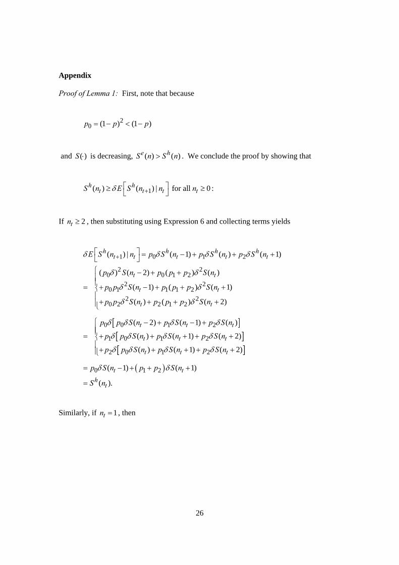
Appendix Proof of Lemma 1: First, note that because

20 (1 ) (1 )p p p= − < −

and ( )S ⋅ is decreasing, ( ) ( )e hS n S n> . We conclude the proof by showing that

1( ) ( ) | for all 0 :h ht t t tS n E S n n nδ +⎡ ⎤≥ ≥⎣ ⎦

If 2tn ≥ , then substituting using Expression 6 and collecting terms yields

1 0 1 2

2 20 0 1 2

2 20 1 1 1 2

2 20 2 2 1 2

( ) | ( 1) ( ) ( 1)

( ) ( 2) ( ) ( )

( 1) ( ) ( 1)

( ) ( ) ( 2)

h h h ht t t t t

t t

t t

t t

E S n n p S n p S n p S n

p S n p p p S n

p p S n p p p S n

p p S n p p p S n

δ δ δ δ

δ δ

δ δ

δ δ

+⎡ ⎤ = − + + +⎣ ⎦⎧ − + +⎪⎪= + − + + +⎨⎪+ + + +⎪⎩

[ ][ ][ ]

0 0 1 2

1 0 1 2

2 0 1 2

( 2) ( 1) ( )

( ) ( 1) ( 2)

( ) ( 1) ( 2)

t t t

t t t

t t t

p p S n p S n p S n

p p S n p S n p S n

p p S n p S n p S n

δ δ δ δ

δ δ δ δ

δ δ δ δ

⎧ − + − +⎪⎪= + + + + +⎨⎪+ + + + +⎪⎩

( )0 1 2( 1) ( 1)

( ).

t th

t

p S n p p S n

S n

δ δ= − + + +

=

Similarly, if 1tn = , then

27

[ ][ ][ ]

1 0 1 2

0 0 1 2

1 0 1 2

2 0 1 2

( ) | 1 (0) (1) (2)

( ) ( ) (1)

(1) (2) (3)

(1) (2) (3)

h h h ht t

H H

E S n n p S p S p S

p p V R p V R p S

p p S p S p S

p p S p S p S

δ δ δ δ

δ δ

δ δ δ δ

δ δ δ δ

+⎡ ⎤= = + +⎣ ⎦⎧ − + − +⎪⎪= + + +⎨⎪+ + +⎪⎩

[ ] ( )0 0 1 2 1 2( )( ) (1) (2)

(1),

Hh

p p p V R p S p p S

S

δ δ δ= + − + + +

<

and if 0tn = , then

1 0 1 2( ) | 0 ( ) (0) (1)

(0).

h h ht t

h

E S n n p p S p S

S

δ δ δ+⎡ ⎤= = + +⎣ ⎦

<

Thus,

1( ) ( ) | for all 0.h ht t tS n E S n n nδ +

⎡ ⎤≥ ≥⎣ ⎦ Q.E.D.

28

FIGURES AND TABLES

Table 1: Definitions of variables

Variables Explanation

Auction number ID of the auction

Winning bid Maximum recorded bid of each auction

Starting bid Starting price of the auction that is set by the seller

Minimum bid Minimum recorded bid of each auction

Auction length (hr) Length of the auction measured in hours

Number of bids Total number of bids at the end of the auction

Number of bidders Total number of bidders at the end of the auction

I Total number of unsuccessful bidders in previous 10 auctions

Table 2: Descriptive statistics for TI-83 calculators

Variable Num.

of Obs. Mean Median

Std.

Dev. Min Max

Winning bid 1817 58.21 53.09 17. 7 20 107.52

Starting bid 1817 15.07 9.99 15.96 0.01 99.99

Minimum bid 1817 18.74 12 16.65 0.01 99.99

Auction length

(hr) 1817 135.3 168 46.25 72 240

Number of

bids 1817 13.7 13 7.04 1 54

Number of

bidders 1817 7.29 7 3.02 1 18

I 1807 62.83 62 13.14 12 115

29

Table 3: Summary statistics for the closing intervals

Variable Num. of

Obs. Mean Median

Std.

Dev. Min Max

Closing Interval

(minutes) 1816 33.59 14 64.92 0 714

Table 4: Distribution of closing intervals with various lengths

Minutes in the Closing Interval Frequency Percent (%) Cumulative (%)

0 112 6.17 6.17

1 132 7.27 13.44

2 79 4.35 17.79

3 84 4.63 22.41

4 69 3.80 26.21

5 62 3.41 29.63

6-10 238 13.1 42.73

11-30 538 29.63 72.36

>30 502 27.64 100

30

Table 5: Number of bidders and number of auctions that they won

Number of wins Number of bidders Percentage

0 355 49%

1 310 43%

2 39

3 9

4 2

5 1

6 1

10 1

15 1

49 1

8%

Table 6: Regression of winning bid on number of incumbents

2SLS Winning Bid OLS

First-stage regression IV regression

I 0.1531*** (0.0337) ---- 0.6972**

(0.3169)

Closing Interval ---- 0.0086* (0.0046)

0.0074 (0.0097)

Elapsed Time ---- 0.0075*** (0.0016) ----

Constant 45.9101*** (5.6704)

49.7893*** (3.2217)

16.6457 (17.7278)

R-squared 0.0391 0.1452 ---- Wald Chi-squared (31) ---- ---- 61.58 Number of Observations: 1806

Notes: *** indicates significance at 1% level. ** indicates significance at 5% level. * indicates significance at 10% level. Hour and day dummies were also included as regressors.

31

Figure 1: Bid submission times in the closing intervals

Figure 2: Bid Submission times in the closing intervals, by incumbent status

0

.05

.1

.15

.2

0 .5 1 0 .5 1

Entrants Incumbents

Frac

tion

Fraction of all bids & all intervals

32

0

.05

.1

.15

.2

0 .5 1 0 .5 1

Entrants Incumbents

Frac

tion

Fraction of all bids & intervals greater than 1 minute

0

.1

.2

0 .5 1 0 .5 1

Entrants Incumbents

Frac

tion

Fraction of all bids & intervals greater than 3 minutes

33

Figure 3: Bidder behavior in consecutive auctions

0

.1

.2

0 .5 1 0 .5 1

Entrants Incumbents

Frac

tion

Fraction of all bids & intervals greater than 5 minutes

W

W W

L

L L

E E

E B

B B

E B E B E B

720

135 585

25 110 156 429

9 16 63 366

4 5 7 9 53 10 50 316

First auction

Second auction