Latency Inflation with MPLS-based Traffic Engineering

Abhinav PathakPurdue University

pathaka@purdue.edu

Ming ZhangMicrosoft Research

mzh@microsoft.com

Y. Charlie HuPurdue University

ychu@purdue.edu

Ratul MahajanMicrosoft Research

ratul@microsoft.com

Dave MaltzMicrosoft Research

dmaltz@microsoft.com

ABSTRACTWhile MPLS has been extensively deployed in recent years, lit-tle is known about its behavior in practice. We examine the per-formance of MPLS in Microsoft’s online service network (MSN),a well-provisioned multi-continent production network connectingtens of data centers. Using detailed traces collected over a 2-monthperiod, we find that many paths experience significantly inflated la-tencies. We correlate occurrences of latency inflation with routers,links, and DC-pairs. This analysis sheds light on the causes oflatency inflation and suggests several avenues for alleviating theproblem.

Categories and Subject DescriptorsC.4 [Performance of Systems]: Performance Attributes

General TermsMeasurement, Performance

KeywordsMPLS, LSP, Autobandwidth, Latency

1. INTRODUCTIONTraffic engineering (TE) is the process of deciding how traffic

is routed through the service provider network. Its goal is to ac-commodate the given traffic matrix (from ingress to egress routers)while optimizing for performance objectives of low latency andloss rate. Effective TE mechanisms are key to efficiently using net-work resources and maintaining good performance for traffic.

The importance of TE has motivated the development of manyschemes (e.g., [5, 7]), but little is known today about the effective-ness or behavior of schemes that have been deployed in practice.Much of the prior work is based on various forms of simulationsand emulations rather than based on real measurements taken froman operational network.

In this paper, we present a case study of the behavior of TE asdeployed in a large network. This network (MSN) is the one thatconnects Microsoft’s data centers to each other and to peering ISPs.

Permission to make digital or hard copies of all or part of this work forpersonal or classroom use is granted without fee provided that copies arenot made or distributed for profit or commercial advantage and that copiesbear this notice and the full citation on the first page. To copy otherwise, torepublish, to post on servers or to redistribute to lists, requires prior specificpermission and/or a fee.IMC’11, November 2–4, 2011, Berlin, Germany.Copyright 2011 ACM 978-1-4503-1013-0/11/11 ...$10.00.

0

20

40

60

80

100

Oct 15 Nov 1 Nov 15

OW

D(m

s)

Timeline

Figure 1: Tunnel latency during one month period

MSN uses MPLS-based TE, which is perhaps the most widely usedTE mechanism and is supported by major router vendors such asCisco and Juniper. Although we use MSN as a case study, we be-lieve that our findings are general because the behaviors we un-cover are tied to the MPLS-TE algorithms themselves rather thanto MSN. The contribution of our work lies in uncovering and quan-tifying problems with MPLS-TE in a production network, as a firststep towards improving the TE algorithms.

Our interest in studying the behavior of MPLS-TE was not purelyacademic but was motivated by anomalous behavior observed bythe operators of Bing Search which uses the MSN network. Dur-ing the period of our study, Bing Search experienced incidents ofunexpectedly high latencies between two of its DCs from time totime. Because these two DCs are in the same city, Bing’s opera-tions expected the latency between them to be negligible. In fact,this assumption is also made by Bing’s planning team when theychose to distribute Bing’s backend services across the two DCs.

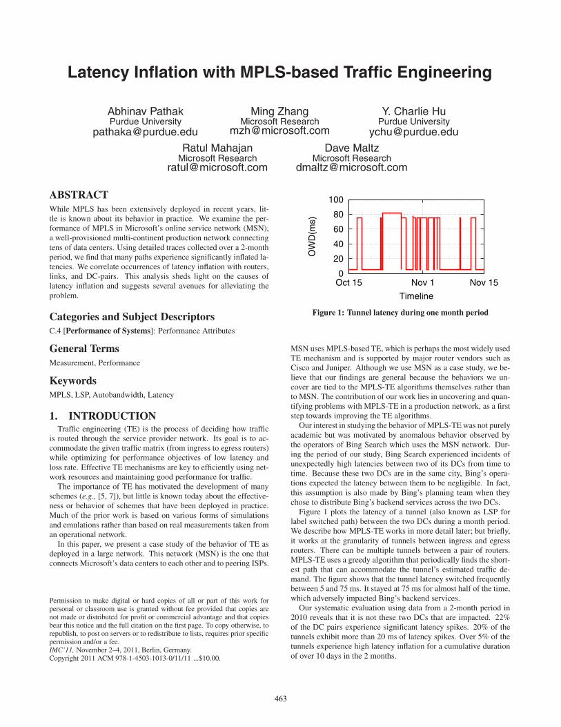
Figure 1 plots the latency of a tunnel (also known as LSP forlabel switched path) between the two DCs during a month period.We describe how MPLS-TE works in more detail later; but briefly,it works at the granularity of tunnels between ingress and egressrouters. There can be multiple tunnels between a pair of routers.MPLS-TE uses a greedy algorithm that periodically finds the short-est path that can accommodate the tunnel’s estimated traffic de-mand. The figure shows that the tunnel latency switched frequentlybetween 5 and 75 ms. It stayed at 75 ms for almost half of the time,which adversely impacted Bing’s backend services.

Our systematic evaluation using data from a 2-month period in2010 reveals that it is not these two DCs that are impacted. 22%of the DC pairs experience significant latency spikes. 20% of thetunnels exhibit more than 20 ms of latency spikes. Over 5% of thetunnels experience high latency inflation for a cumulative durationof over 10 days in the 2 months.

463

Figure 2: OSP network topology

To gain insight into the causes for latency inflation, we correlatesuch occurrences with specific links, routers, and DC pairs. Ouranalysis shows that 80% of latency inflation occur due to changesin tunnel paths concentrated on 9% of the links, 30% of the routers,and 3% of the active DC-pairs. This confirms traffic load changesexceeding the capacity of a small set of links along the shortestpaths of tunnels as the primary culprit. MSN operators have sinceadded capacity along these paths to alleviate the problem.

But to understand the effectiveness of MPLS at using availableresources, we compare the latency with MPLS-TE to that with anoptimal strategy based on linear programming. We find that theweighted and the 99th percentile byte latency under MPLS-TE are10%-22% and 35%-40% higher than that under optimal routingstrategy, respectively, suggesting there exists room for improve-ment under MPLS-TE.

We identify several problems caused by sub-optimal setting ofMPLS parameters but leave as future work automatic parametersetting and on-the-fly LSP split as two methods to fix the latencyinflation problem.

2. BACKGROUNDA service provider network is composed of multiple points-of-

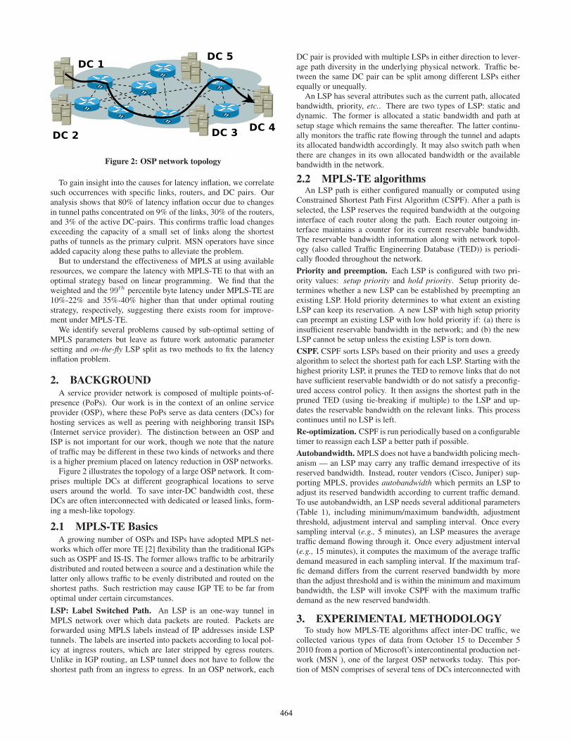
presence (PoPs). Our work is in the context of an online serviceprovider (OSP), where these PoPs serve as data centers (DCs) forhosting services as well as peering with neighboring transit ISPs(Internet service provider). The distinction between an OSP andISP is not important for our work, though we note that the natureof traffic may be different in these two kinds of networks and thereis a higher premium placed on latency reduction in OSP networks.

Figure 2 illustrates the topology of a large OSP network. It com-prises multiple DCs at different geographical locations to serveusers around the world. To save inter-DC bandwidth cost, theseDCs are often interconnected with dedicated or leased links, form-ing a mesh-like topology.

2.1 MPLS-TE BasicsA growing number of OSPs and ISPs have adopted MPLS net-

works which offer more TE [2] flexibility than the traditional IGPssuch as OSPF and IS-IS. The former allows traffic to be arbitrarilydistributed and routed between a source and a destination while thelatter only allows traffic to be evenly distributed and routed on theshortest paths. Such restriction may cause IGP TE to be far fromoptimal under certain circumstances.

LSP: Label Switched Path. An LSP is an one-way tunnel inMPLS network over which data packets are routed. Packets areforwarded using MPLS labels instead of IP addresses inside LSPtunnels. The labels are inserted into packets according to local pol-icy at ingress routers, which are later stripped by egress routers.Unlike in IGP routing, an LSP tunnel does not have to follow theshortest path from an ingress to egress. In an OSP network, each

DC pair is provided with multiple LSPs in either direction to lever-age path diversity in the underlying physical network. Traffic be-tween the same DC pair can be split among different LSPs eitherequally or unequally.

An LSP has several attributes such as the current path, allocatedbandwidth, priority, etc.. There are two types of LSP: static anddynamic. The former is allocated a static bandwidth and path atsetup stage which remains the same thereafter. The latter continu-ally monitors the traffic rate flowing through the tunnel and adaptsits allocated bandwidth accordingly. It may also switch path whenthere are changes in its own allocated bandwidth or the availablebandwidth in the network.

2.2 MPLS-TE algorithmsAn LSP path is either configured manually or computed using

Constrained Shortest Path First Algorithm (CSPF). After a path isselected, the LSP reserves the required bandwidth at the outgoinginterface of each router along the path. Each router outgoing in-terface maintains a counter for its current reservable bandwidth.The reservable bandwidth information along with network topol-ogy (also called Traffic Engineering Database (TED)) is periodi-cally flooded throughout the network.

Priority and preemption. Each LSP is configured with two pri-ority values: setup priority and hold priority. Setup priority de-termines whether a new LSP can be established by preempting anexisting LSP. Hold priority determines to what extent an existingLSP can keep its reservation. A new LSP with high setup prioritycan preempt an existing LSP with low hold priority if: (a) there isinsufficient reservable bandwidth in the network; and (b) the newLSP cannot be setup unless the existing LSP is torn down.

CSPF. CSPF sorts LSPs based on their priority and uses a greedyalgorithm to select the shortest path for each LSP. Starting with thehighest priority LSP, it prunes the TED to remove links that do nothave sufficient reservable bandwidth or do not satisfy a preconfig-ured access control policy. It then assigns the shortest path in thepruned TED (using tie-breaking if multiple) to the LSP and up-dates the reservable bandwidth on the relevant links. This processcontinues until no LSP is left.

Re-optimization. CSPF is run periodically based on a configurabletimer to reassign each LSP a better path if possible.

Autobandwidth. MPLS does not have a bandwidth policing mech-anism — an LSP may carry any traffic demand irrespective of itsreserved bandwidth. Instead, router vendors (Cisco, Juniper) sup-porting MPLS, provides autobandwidth which permits an LSP toadjust its reserved bandwidth according to current traffic demand.To use autobandwidth, an LSP needs several additional parameters(Table 1), including minimum/maximum bandwidth, adjustmentthreshold, adjustment interval and sampling interval. Once everysampling interval (e.g., 5 minutes), an LSP measures the averagetraffic demand flowing through it. Once every adjustment interval(e.g., 15 minutes), it computes the maximum of the average trafficdemand measured in each sampling interval. If the maximum traf-fic demand differs from the current reserved bandwidth by morethan the adjust threshold and is within the minimum and maximumbandwidth, the LSP will invoke CSPF with the maximum trafficdemand as the new reserved bandwidth.

3. EXPERIMENTAL METHODOLOGYTo study how MPLS-TE algorithms affect inter-DC traffic, we

collected various types of data from October 15 to December 52010 from a portion of Microsoft’s intercontinental production net-work (MSN ), one of the largest OSP networks today. This por-tion of MSN comprises of several tens of DCs interconnected with

464

Table 1: Autobandwidth parametersParameter DescriptionSubscription factor % of interface bandwidth that can be reservedAdjust interval Time interval to trigger autobandwidthAdjust threshold % of change in reserved bandwidth to trigger

autobandwidthMin/max bw Bandwidth limits of an LSPSetup/hold priority Priorities for determining LSP preemption

high-speed dedicated links with the core of network in US. All theinter-DC traffic is carried over 5K LSPs, each using autobandwidth,with 1-32 LSPs between each pair of DC. The data contains net-work topology and router and LSP configurations. For each LSP,it also contains each path change event and traffic volume in each5-minute sampling interval.

Measuring LSP latency is a challenging task for two reasons (a)LSPs are unidirectional; as a result a simple ping would return One-Way Delay (OWD) latencies of two LSPs (the forward LSP and thereverse direction LSP). Separating out the two latencies would re-quire strict time synchronization between the probers across DCs(b) Traffic between a DC pair is load balanced using hashing algo-rithms on all the LSPs (between 1 to 30) between the DCs. Hashfunctions are based on IP/TCP or even application level headers.As a result, to probe all the LSPs between a DC pair using simpleping, we must have one prober covering all the possible IP rangesallocated as well as a applications running in DCs.

Another way to measure LSP latency is to use LSP ping [6, 9].However, because LSP ping is disabled in MSN , we choose toestimate LSP latency based on the geographical locations of therouters along an LSP path. Given an LSP, we calculate the great-circle distance between each pair of intermediate routers and sumit up to obtain the total geographical distance of the LSP. We thendividing the total distance by the speed of light in fiber to obtainthe LSP latency. We verified for a few LSPs that the conversionindeed estimates correct delay with minimal error. Note that LSP isunidirectional, as a result, the latency measured in this mechanismis One-Way-Delay (OWD) estimation.

4. LSP LATENCY INFLATIONIn this section we first describe the severity of the latency prob-

lem in an MPLS based network and then correlate latency inducingLSP path changes with dc pairs, routers and links in the network.

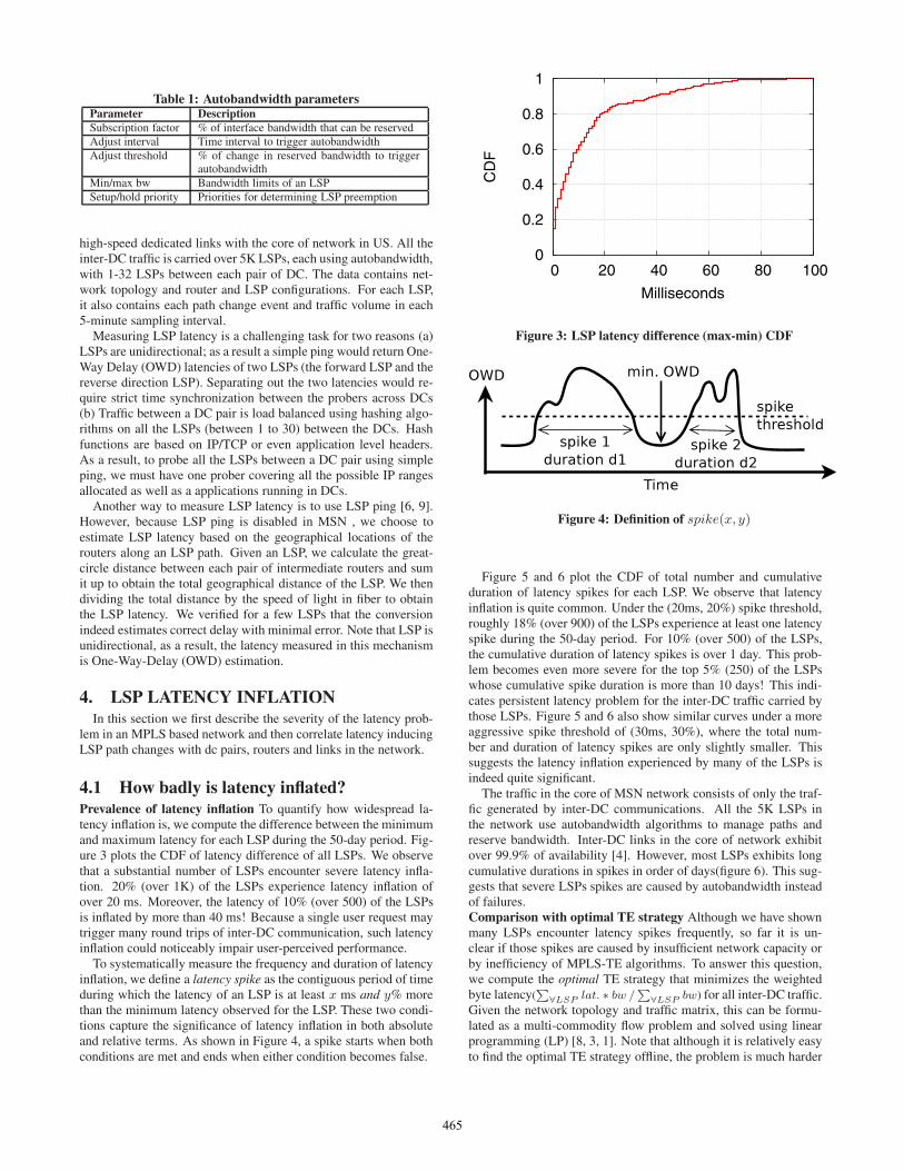
4.1 How badly is latency inflated?Prevalence of latency inflation To quantify how widespread la-tency inflation is, we compute the difference between the minimumand maximum latency for each LSP during the 50-day period. Fig-ure 3 plots the CDF of latency difference of all LSPs. We observethat a substantial number of LSPs encounter severe latency infla-tion. 20% (over 1K) of the LSPs experience latency inflation ofover 20 ms. Moreover, the latency of 10% (over 500) of the LSPsis inflated by more than 40 ms! Because a single user request maytrigger many round trips of inter-DC communication, such latencyinflation could noticeably impair user-perceived performance.

To systematically measure the frequency and duration of latencyinflation, we define a latency spike as the contiguous period of timeduring which the latency of an LSP is at least x ms and y% morethan the minimum latency observed for the LSP. These two condi-tions capture the significance of latency inflation in both absoluteand relative terms. As shown in Figure 4, a spike starts when bothconditions are met and ends when either condition becomes false.

0

0.2

0.4

0.6

0.8

1

0 20 40 60 80 100

CD

F

Milliseconds

Figure 3: LSP latency difference (max-min) CDF

Figure 4: Definition of spike(x, y)

Figure 5 and 6 plot the CDF of total number and cumulativeduration of latency spikes for each LSP. We observe that latencyinflation is quite common. Under the (20ms, 20%) spike threshold,roughly 18% (over 900) of the LSPs experience at least one latencyspike during the 50-day period. For 10% (over 500) of the LSPs,the cumulative duration of latency spikes is over 1 day. This prob-lem becomes even more severe for the top 5% (250) of the LSPswhose cumulative spike duration is more than 10 days! This indi-cates persistent latency problem for the inter-DC traffic carried bythose LSPs. Figure 5 and 6 also show similar curves under a moreaggressive spike threshold of (30ms, 30%), where the total num-ber and duration of latency spikes are only slightly smaller. Thissuggests the latency inflation experienced by many of the LSPs isindeed quite significant.

The traffic in the core of MSN network consists of only the traf-fic generated by inter-DC communications. All the 5K LSPs inthe network use autobandwidth algorithms to manage paths andreserve bandwidth. Inter-DC links in the core of network exhibitover 99.9% of availability [4]. However, most LSPs exhibits longcumulative durations in spikes in order of days(figure 6). This sug-gests that severe LSPs spikes are caused by autobandwidth insteadof failures.Comparison with optimal TE strategy Although we have shownmany LSPs encounter latency spikes frequently, so far it is un-clear if those spikes are caused by insufficient network capacity orby inefficiency of MPLS-TE algorithms. To answer this question,we compute the optimal TE strategy that minimizes the weightedbyte latency(

∑∀LSP lat. ∗ bw /

∑∀LSP bw) for all inter-DC traffic.

Given the network topology and traffic matrix, this can be formu-lated as a multi-commodity flow problem and solved using linearprogramming (LP) [8, 3, 1]. Note that although it is relatively easyto find the optimal TE strategy offline, the problem is much harder

465

0.8

0.82

0.84

0.86

0.88

0.9

0.92

0.94

0.96

0.98

1

0 5 10 15 20

CD

F

Number of Spikes

(20ms, 20%)(30ms, 30%)

Figure 5: CDF of number of spikes observed by LSPs for differentvalues of spikes

0.8

0.82

0.84

0.86

0.88

0.9

0.92

0.94

0.96

0.98

1

0 5 10 15 20

CD

F

Cummulative duration (days)

(20ms, 20%)(30ms, 30%)

Figure 6: CDF of cumulative duration of spikes observed by LSPsfor different values of spikes

to tackle online due to the of size of the topology (resulting in mil-lion variable LP) and volatility traffic demand.

We divide the time into 5-minute intervals and compute the op-timal TE strategy for each interval using the method stated above.Compared to optimal routing, we found that MPLS based routingincurs an overall 10% to 22% increase in weighted byte latencyover different snapshots spanning over a one day period. Figure 7compares the latency at different traffic volume percentile underthe optimal and MPLS-TE in a typical interval. There is substan-tial latency gap between the two TE strategies — the relative la-tency difference stays above 30% (y2 axis) at 50th, 90th, 95th, and99th-percentile of traffic volume. Figure 8 plots the latency at the99th-percentile of traffic volume under both TE strategies during anentire day. Except between midnight and early morning hour, thelatency under MPLS-TE is consistently 20 ms (35%-40%) largerthan that under the optimal TE, leaving enough space for improve-ment.

4.2 Is there a pattern in latency inflation?LSP latency inflation is triggered by an LSP switching from a

short to a long path. We now study the patterns of LSP path changesto see if they cluster at certain links, routers, DC pairs or time peri-ods. Although there are many LSP path changes, we consider onlythose that cause a latency spike (e.g.,, latency jumps by more than20 ms and 20%) and call them LLPC’s (large latency path changes).We ignore the remaining path changes since they either have little

Figure 7: Byte latency bar chart for LSP and LP

Figure 8: 99th percentile byte latency under MPLS (LSP)and Optimal Routing (LP)

impact on latency or reduce latency. For an LLPC, we attribute itto the old path rather than the new one because it is triggered byinsufficient bandwidth on the former.

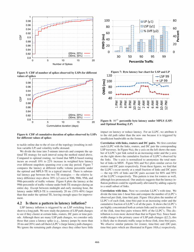
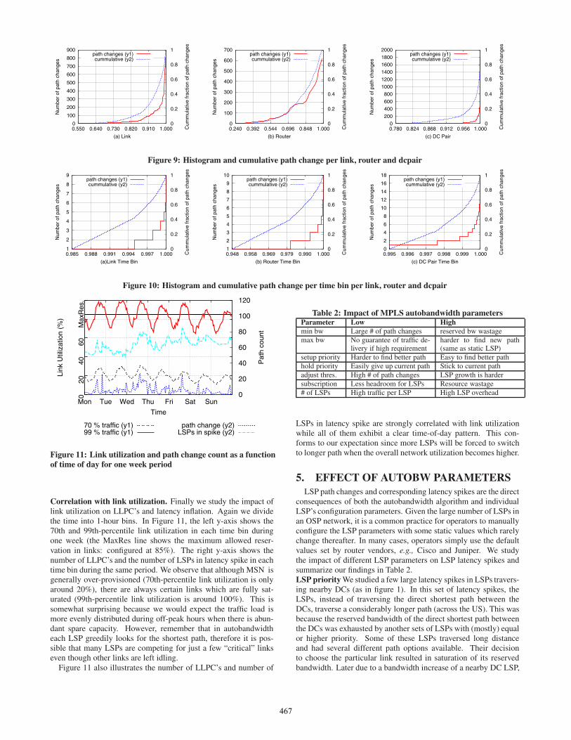
Correlation with links, routers and DC pairs. We first correlateeach LLPC with the links, routers, and DC pair the correspondingLSP traverses. In Figure 9(a), the y-axis on the left shows the num-ber of LLPC’s per link sorted in an increasing order and the y-axison the right shows the cumulative fraction of LLPC’s observed bythe links. The x-axis is normalized to anonymize the total num-ber of links in MSN . Figure 9(b) and 9(c) plots similar curves forrouters and DC pairs respectively. From these figures, we find thatthe LLPC’s occur mostly at a small fraction of links and DC pairs— the top 10% of links and DC pairs account for 80% and 95%of the LLPC’s respectively. This pattern is true for routers as well,although less pronounced. Our analysis suggests that the latency in-flation problem could be significantly alleviated by adding capacityto a small subset of links.

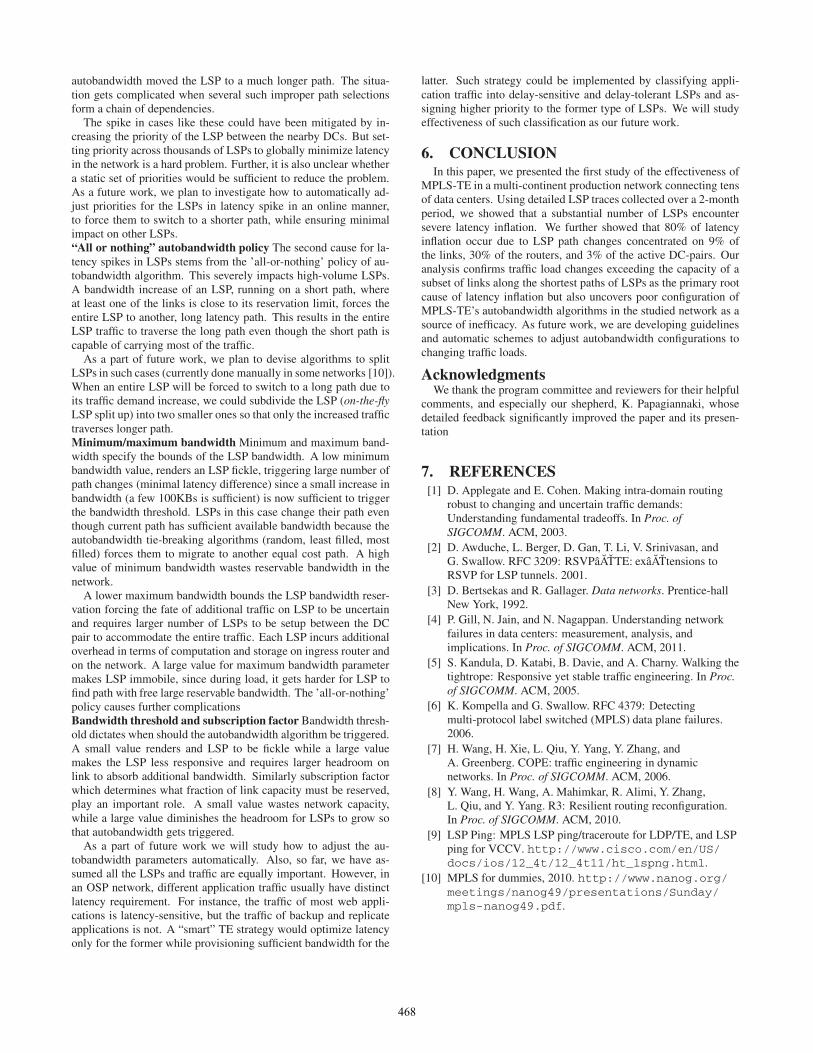
Correlation with time. Next we correlate LLPC’s with time. Wedivide the time into 1-hour bins and compute the number of LLPC’sobserved per (link, time-bin) pair. Figure 10(a) plots the number ofLLPC’s of each (link, time-bin) pair in an increasing order and thecumulative fraction of LLPC’s of all the pairs. It shows the LLPC’sare highly concentrated both at certain links and in certain time. 1%of the (link, time-bin) pairs witness 80% of the LLPC’s. This dis-tribution is even more skewed than that in Figure 9(a). Since band-width change is the primary cause of LSP path changes (§2.2), thisis likely due to dramatic traffic surge in those (link, time-bin) pairs.We observe similar patterns for (router, time-bin) and (DC-pair,time-bin) pairs which are illustrated in Figure 10(b,c) respectively.

466

0

100

200

300

400

500

600

700

800

900

0.550 0.640 0.730 0.820 0.910 1.000 0

0.2

0.4

0.6

0.8

1N

umbe

r of

pat

h ch

ange

s

Cum

mul

ativ

e fr

actio

n of

pat

h ch

ange

s

(a) Link

path changes (y1)cummulative (y2)

0

100

200

300

400

500

600

700

0.240 0.392 0.544 0.696 0.848 1.000 0

0.2

0.4

0.6

0.8

1

Num

ber

of p

ath

chan

ges

Cum

mul

ativ

e fr

actio

n of

pat

h ch

ange

s

(b) Router

path changes (y1)cummulative (y2)

0

200 400

600

800

1000 1200

1400

1600 1800

2000

0.780 0.824 0.868 0.912 0.956 1.000 0

0.2

0.4

0.6

0.8

1

Num

ber

of p

ath

chan

ges

Cum

mul

ativ

e fr

actio

n of

pat

h ch

ange

s

(c) DC Pair

path changes (y1)cummulative (y2)

Figure 9: Histogram and cumulative path change per link, router and dcpair

1

2

3

4

5

6

7

8

9

0.985 0.988 0.991 0.994 0.997 1.000 0

0.2

0.4

0.6

0.8

1

Num

ber

of p

ath

chan

ges

Cum

mul

ativ

e fr

actio

n of

pat

h ch

ange

s

(a)Link Time Bin

path changes (y1)cummulative (y2)

1

2

3

4

5

6

7

8

9

10

0.948 0.958 0.969 0.979 0.990 1.000 0

0.2

0.4

0.6

0.8

1

Num

ber

of p

ath

chan

ges

Cum

mul

ativ

e fr

actio

n of

pat

h ch

ange

s

(b) Router Time Bin

path changes (y1)cummulative (y2)

0

2

4

6

8

10

12

14

16

18

0.995 0.996 0.997 0.998 0.999 1.000 0

0.2

0.4

0.6

0.8

1

Num

ber

of p

ath

chan

ges

Cum

mul

ativ

e fr

actio

n of

pat

h ch

ange

s

(c) DC Pair Time Bin

path changes (y1)cummulative (y2)

Figure 10: Histogram and cumulative path change per time bin per link, router and dcpair

020

4060

Max

Res

.

Mon Tue Wed Thu Fri Sat Sun 0

20

40

60

80

100

120

Link

Util

izat

ion

(%)

Pat

h co

unt

Time

70 % traffic (y1)99 % traffic (y1)

path change (y2)LSPs in spike (y2)

Figure 11: Link utilization and path change count as a functionof time of day for one week period

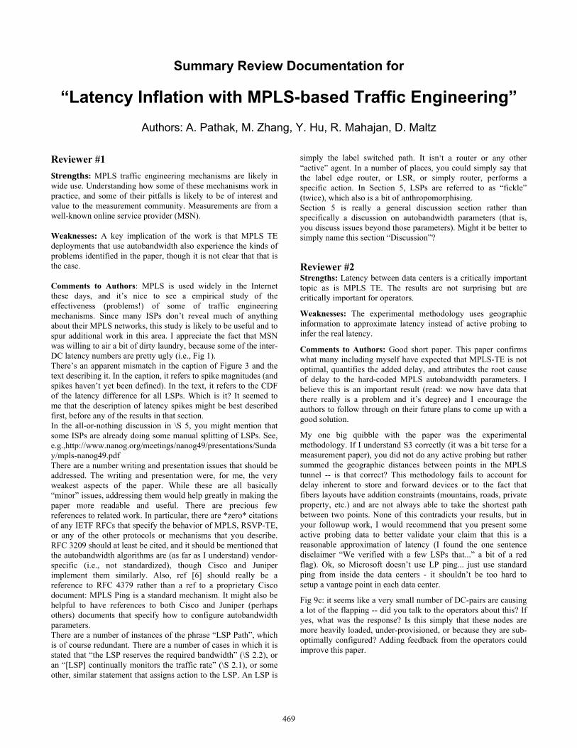
Correlation with link utilization. Finally we study the impact oflink utilization on LLPC’s and latency inflation. Again we dividethe time into 1-hour bins. In Figure 11, the left y-axis shows the70th and 99th-percentile link utilization in each time bin duringone week (the MaxRes line shows the maximum allowed reser-vation in links: configured at 85%). The right y-axis shows thenumber of LLPC’s and the number of LSPs in latency spike in eachtime bin during the same period. We observe that although MSN isgenerally over-provisioned (70th-percentile link utilization is onlyaround 20%), there are always certain links which are fully sat-urated (99th-percentile link utilization is around 100%). This issomewhat surprising because we would expect the traffic load ismore evenly distributed during off-peak hours when there is abun-dant spare capacity. However, remember that in autobandwidtheach LSP greedily looks for the shortest path, therefore it is pos-sible that many LSPs are competing for just a few “critical” linkseven though other links are left idling.

Figure 11 also illustrates the number of LLPC’s and number of

Table 2: Impact of MPLS autobandwidth parametersParameter Low Highmin bw Large # of path changes reserved bw wastagemax bw No guarantee of traffic de-

livery if high requirementharder to find new path(same as static LSP)

setup priority Harder to find better path Easy to find better pathhold priority Easily give up current path Stick to current pathadjust thres. High # of path changes LSP growth is hardersubscription Less headroom for LSPs Resource wastage# of LSPs High traffic per LSP High LSP overhead

LSPs in latency spike are strongly correlated with link utilizationwhile all of them exhibit a clear time-of-day pattern. This con-forms to our expectation since more LSPs will be forced to switchto longer path when the overall network utilization becomes higher.

5. EFFECT OF AUTOBW PARAMETERSLSP path changes and corresponding latency spikes are the direct

consequences of both the autobandwidth algorithm and individualLSP’s configuration parameters. Given the large number of LSPs inan OSP network, it is a common practice for operators to manuallyconfigure the LSP parameters with some static values which rarelychange thereafter. In many cases, operators simply use the defaultvalues set by router vendors, e.g., Cisco and Juniper. We studythe impact of different LSP parameters on LSP latency spikes andsummarize our findings in Table 2.LSP priority We studied a few large latency spikes in LSPs travers-ing nearby DCs (as in figure 1). In this set of latency spikes, theLSPs, instead of traversing the direct shortest path between theDCs, traverse a considerably longer path (across the US). This wasbecause the reserved bandwidth of the direct shortest path betweenthe DCs was exhausted by another sets of LSPs with (mostly) equalor higher priority. Some of these LSPs traversed long distanceand had several different path options available. Their decisionto choose the particular link resulted in saturation of its reservedbandwidth. Later due to a bandwidth increase of a nearby DC LSP,

467

autobandwidth moved the LSP to a much longer path. The situa-tion gets complicated when several such improper path selectionsform a chain of dependencies.

The spike in cases like these could have been mitigated by in-creasing the priority of the LSP between the nearby DCs. But set-ting priority across thousands of LSPs to globally minimize latencyin the network is a hard problem. Further, it is also unclear whethera static set of priorities would be sufficient to reduce the problem.As a future work, we plan to investigate how to automatically ad-just priorities for the LSPs in latency spike in an online manner,to force them to switch to a shorter path, while ensuring minimalimpact on other LSPs.“All or nothing” autobandwidth policy The second cause for la-tency spikes in LSPs stems from the ’all-or-nothing’ policy of au-tobandwidth algorithm. This severely impacts high-volume LSPs.A bandwidth increase of an LSP, running on a short path, whereat least one of the links is close to its reservation limit, forces theentire LSP to another, long latency path. This results in the entireLSP traffic to traverse the long path even though the short path iscapable of carrying most of the traffic.

As a part of future work, we plan to devise algorithms to splitLSPs in such cases (currently done manually in some networks [10]).When an entire LSP will be forced to switch to a long path due toits traffic demand increase, we could subdivide the LSP (on-the-flyLSP split up) into two smaller ones so that only the increased traffictraverses longer path.Minimum/maximum bandwidth Minimum and maximum band-width specify the bounds of the LSP bandwidth. A low minimumbandwidth value, renders an LSP fickle, triggering large number ofpath changes (minimal latency difference) since a small increase inbandwidth (a few 100KBs is sufficient) is now sufficient to triggerthe bandwidth threshold. LSPs in this case change their path eventhough current path has sufficient available bandwidth because theautobandwidth tie-breaking algorithms (random, least filled, mostfilled) forces them to migrate to another equal cost path. A highvalue of minimum bandwidth wastes reservable bandwidth in thenetwork.

A lower maximum bandwidth bounds the LSP bandwidth reser-vation forcing the fate of additional traffic on LSP to be uncertainand requires larger number of LSPs to be setup between the DCpair to accommodate the entire traffic. Each LSP incurs additionaloverhead in terms of computation and storage on ingress router andon the network. A large value for maximum bandwidth parametermakes LSP immobile, since during load, it gets harder for LSP tofind path with free large reservable bandwidth. The ’all-or-nothing’policy causes further complicationsBandwidth threshold and subscription factor Bandwidth thresh-old dictates when should the autobandwidth algorithm be triggered.A small value renders and LSP to be fickle while a large valuemakes the LSP less responsive and requires larger headroom onlink to absorb additional bandwidth. Similarly subscription factorwhich determines what fraction of link capacity must be reserved,play an important role. A small value wastes network capacity,while a large value diminishes the headroom for LSPs to grow sothat autobandwidth gets triggered.

As a part of future work we will study how to adjust the au-tobandwidth parameters automatically. Also, so far, we have as-sumed all the LSPs and traffic are equally important. However, inan OSP network, different application traffic usually have distinctlatency requirement. For instance, the traffic of most web appli-cations is latency-sensitive, but the traffic of backup and replicateapplications is not. A “smart” TE strategy would optimize latencyonly for the former while provisioning sufficient bandwidth for the

latter. Such strategy could be implemented by classifying appli-cation traffic into delay-sensitive and delay-tolerant LSPs and as-signing higher priority to the former type of LSPs. We will studyeffectiveness of such classification as our future work.

6. CONCLUSIONIn this paper, we presented the first study of the effectiveness of

MPLS-TE in a multi-continent production network connecting tensof data centers. Using detailed LSP traces collected over a 2-monthperiod, we showed that a substantial number of LSPs encountersevere latency inflation. We further showed that 80% of latencyinflation occur due to LSP path changes concentrated on 9% ofthe links, 30% of the routers, and 3% of the active DC-pairs. Ouranalysis confirms traffic load changes exceeding the capacity of asubset of links along the shortest paths of LSPs as the primary rootcause of latency inflation but also uncovers poor configuration ofMPLS-TE’s autobandwidth algorithms in the studied network as asource of inefficacy. As future work, we are developing guidelinesand automatic schemes to adjust autobandwidth configurations tochanging traffic loads.

AcknowledgmentsWe thank the program committee and reviewers for their helpful

comments, and especially our shepherd, K. Papagiannaki, whosedetailed feedback significantly improved the paper and its presen-tation

7. REFERENCES[1] D. Applegate and E. Cohen. Making intra-domain routing

robust to changing and uncertain traffic demands:Understanding fundamental tradeoffs. In Proc. ofSIGCOMM. ACM, 2003.

[2] D. Awduche, L. Berger, D. Gan, T. Li, V. Srinivasan, andG. Swallow. RFC 3209: RSVPâATTE: exâATtensions toRSVP for LSP tunnels. 2001.

[3] D. Bertsekas and R. Gallager. Data networks. Prentice-hallNew York, 1992.

[4] P. Gill, N. Jain, and N. Nagappan. Understanding networkfailures in data centers: measurement, analysis, andimplications. In Proc. of SIGCOMM. ACM, 2011.

[5] S. Kandula, D. Katabi, B. Davie, and A. Charny. Walking thetightrope: Responsive yet stable traffic engineering. In Proc.of SIGCOMM. ACM, 2005.

[6] K. Kompella and G. Swallow. RFC 4379: Detectingmulti-protocol label switched (MPLS) data plane failures.2006.

[7] H. Wang, H. Xie, L. Qiu, Y. Yang, Y. Zhang, andA. Greenberg. COPE: traffic engineering in dynamicnetworks. In Proc. of SIGCOMM. ACM, 2006.

[8] Y. Wang, H. Wang, A. Mahimkar, R. Alimi, Y. Zhang,L. Qiu, and Y. Yang. R3: Resilient routing reconfiguration.In Proc. of SIGCOMM. ACM, 2010.

[9] LSP Ping: MPLS LSP ping/traceroute for LDP/TE, and LSPping for VCCV. http://www.cisco.com/en/US/docs/ios/12_4t/12_4t11/ht_lspng.html.

[10] MPLS for dummies, 2010. http://www.nanog.org/meetings/nanog49/presentations/Sunday/mpls-nanog49.pdf.

468

Summary Review Documentation for

“Latency Inflation with MPLS-based Traffic Engineering”

Authors: A. Pathak, M. Zhang, Y. Hu, R. Mahajan, D. Maltz

Reviewer #1

Strengths: MPLS traffic engineering mechanisms are likely in wide use. Understanding how some of these mechanisms work in practice, and some of their pitfalls is likely to be of interest and value to the measurement community. Measurements are from a well-known online service provider (MSN). Weaknesses: A key implication of the work is that MPLS TE deployments that use autobandwidth also experience the kinds of problems identified in the paper, though it is not clear that that is the case. Comments to Authors: MPLS is used widely in the Internet these days, and it’s nice to see a empirical study of the effectiveness (problems!) of some of traffic engineering mechanisms. Since many ISPs don’t reveal much of anything about their MPLS networks, this study is likely to be useful and to spur additional work in this area. I appreciate the fact that MSN was willing to air a bit of dirty laundry, because some of the inter-DC latency numbers are pretty ugly (i.e., Fig 1). There’s an apparent mismatch in the caption of Figure 3 and the text describing it. In the caption, it refers to spike magnitudes (and spikes haven’t yet been defined). In the text, it refers to the CDF of the latency difference for all LSPs. Which is it? It seemed to me that the description of latency spikes might be best described first, before any of the results in that section. In the all-or-nothing discussion in \S 5, you might mention that some ISPs are already doing some manual splitting of LSPs. See, e.g.,http://www.nanog.org/meetings/nanog49/presentations/Sunday/mpls-nanog49.pdf There are a number writing and presentation issues that should be addressed. The writing and presentation were, for me, the very weakest aspects of the paper. While these are all basically “minor” issues, addressing them would help greatly in making the paper more readable and useful. There are precious few references to related work. In particular, there are *zero* citations of any IETF RFCs that specify the behavior of MPLS, RSVP-TE, or any of the other protocols or mechanisms that you describe. RFC 3209 should at least be cited, and it should be mentioned that the autobandwidth algorithms are (as far as I understand) vendor-specific (i.e., not standardized), though Cisco and Juniper implement them similarly. Also, ref [6] should really be a reference to RFC 4379 rather than a ref to a proprietary Cisco document: MPLS Ping is a standard mechanism. It might also be helpful to have references to both Cisco and Juniper (perhaps others) documents that specify how to configure autobandwidth parameters. There are a number of instances of the phrase “LSP Path”, which is of course redundant. There are a number of cases in which it is stated that “the LSP reserves the required bandwidth” (\S 2.2), or an “[LSP] continually monitors the traffic rate” (\S 2.1), or some other, similar statement that assigns action to the LSP. An LSP is

simply the label switched path. It isn’t a router or any other “active” agent. In a number of places, you could simply say that the label edge router, or LSR, or simply router, performs a specific action. In Section 5, LSPs are referred to as “fickle” (twice), which also is a bit of anthropomorphising. Section 5 is really a general discussion section rather than specifically a discussion on autobandwidth parameters (that is, you discuss issues beyond those parameters). Might it be better to simply name this section “Discussion”?

Reviewer #2 Strengths: Latency between data centers is a critically important topic as is MPLS TE. The results are not surprising but are critically important for operators.

Weaknesses: The experimental methodology uses geographic information to approximate latency instead of active probing to infer the real latency.

Comments to Authors: Good short paper. This paper confirms what many including myself have expected that MPLS-TE is not optimal, quantifies the added delay, and attributes the root cause of delay to the hard-coded MPLS autobandwidth parameters. I believe this is an important result (read: we now have data that there really is a problem and it’s degree) and I encourage the authors to follow through on their future plans to come up with a good solution.

My one big quibble with the paper was the experimental methodology. If I understand S3 correctly (it was a bit terse for a measurement paper), you did not do any active probing but rather summed the geographic distances between points in the MPLS tunnel -- is that correct? This methodology fails to account for delay inherent to store and forward devices or to the fact that fibers layouts have addition constraints (mountains, roads, private property, etc.) and are not always able to take the shortest path between two points. None of this contradicts your results, but in your followup work, I would recommend that you present some active probing data to better validate your claim that this is a reasonable approximation of latency (I found the one sentence disclaimer “We verified with a few LSPs that...” a bit of a red flag). Ok, so Microsoft doesn’t use LP ping... just use standard ping from inside the data centers - it shouldn’t be too hard to setup a vantage point in each data center.

Fig 9c: it seems like a very small number of DC-pairs are causing a lot of the flapping -- did you talk to the operators about this? If yes, what was the response? Is this simply that these nodes are more heavily loaded, under-provisioned, or because they are sub-optimally configured? Adding feedback from the operators could improve this paper.

469

Another point to look (likely in follow up work) at is the 5 minute timer that autobandwidth uses to recalculate routes: if that were decreased and the algorithms made more responsive, is there any additional benefit?

Reviewer #3 Strengths: The first look into MPLS-TE in practice. Nice dataset. Paper shows some problems with current TE implementations that should lead to further research.

Weaknesses: The measurements of latency are not direct and some of the analysis could be a little deeper.

Comments to Authors: This paper presents an interesting study of MPLS-TE. To the best of my knowledge this is the first study of a large-scale production network running MPLS-TE. I feel that I’ve learned more about MPLS-TE and the issues that can arise in practice. I just have a few comments.

From your introduction, it is clear that OSP operations have strict requirements for latency between data centers, could you give some numbers of the ranges of acceptable latencies? It would help people who want to find solutions to the problems you are pointing out.

When you present the network in Sec. 3, it would be nice to give an idea of the geographical spread. You only say that it is intercontinental in the conclusion.

At the last paragraph of Sec. 3, it would be nice to add a small explanation of how you verify that your latency estimation actually matches latency. It is a little disappointing that you can’t get direct measurements of latency (why not just do pings from the data centers?), at least elaborating on the validation would help.

Why do label Figures 4, 7, and 8 with OWD, if earlier you’ve defined latency and that is what you use in the text?

People usually use the term stretch to refer to latency inflation.

Sec. 4.2 talks about correlation, but it uses no metric of statistical correlation. One can kind of see the correlation in the example week in Fig. 11, but the numbers would be more general.

Reviewer #4

Strengths: This is the first paper I know that demonstrates the impact of MPLS TE on latency across a network. The authors show a good understanding of how MPLS TE works and discuss possible reasons behind such a phenomenon.

Weaknesses: Unfortunately, the paper does not really prove that the reason behind the latency increase is the way autobandwidth works. The correlation with utilization is weak at best and there is no significant analysis performed to convince that this is the case - for that reason my assessment would be between a 2 and a 3 with a technical correctness at similar levels.

Comments to Authors: I find that this paper makes an attempt to look into a very interesting problem - that of the performance of traffic engineering mechanisms like MPLS TE. Providers have deployed such a solution in the hope that they will be able to better handle performance in their network, but as the authors mention very little is known as to how successful the employed

mechanisms actually are. Moreover, as the authors demonstrate these mechanisms are typically accompanied by a number of thresholds that network operators rarely change - and reasonably so, since nobody could really estimate the impact of those changes.

Interestingly, this paper shows that employing MPLS-TE can lead to significant increases in latency as compared to shortest paths. A large number of paths inside Microsoft’s Online Service Network are showing spikes in latency, thus affecting the performance of the provided services.

The authors have studied the magnitude of latency increases, the number of data centers that they affect, as well as routers. They have further attempted to correlate it with link utilization with the goal to demonstrate that such latency increases may be due to the reaction of autobandwidth mechanism in high load conditions. Unfortunately, that point is never really proven. I would really have liked to see the authors formulating a hypothesis and testing it according to their data. Showing the result on Figure 11 is by no means a proof of that point. For each time bin they have identified the 70% and 99% percentile load across the network and then counted the number of path changes. They claim that the correlation is high but the presented figure is far from conclusive. I would like to have seen something more precise, where the authors track utilization across the network, the LSP messages that will be triggered for sure if autobandwidth kicks in, and then the precise correlation of that LSP change with the utilization increase in one of the links of the LSP. Otherwise, you have not really shown what you claim.

For that reason, i would say that this paper should only be accepted conditionally and published only if the authors manage to properly demonstrate such a correlation of remove that claim from the paper. You need to define the several causes that could lead to a path change (such as failure, etc) and then clearly test the hypothesis of link utilization being the culprit. Given the novelty of the data set and the rest of the analysis I would not say that this paper is a straight reject.

Finally, the authors compare MPLS TE latency with that obtained through an optimization problem that is never precisely defined. I think it is worth spending some space trying to make the paper self-consistent. What is byte weighted latency.

Reviewer #5 Strengths: This is the very first paper that I have read on the measured performance of MPLS networks. These results would be interesting to network operators.

Weaknesses: The paper simply reported the results in a straightforward way. Rather than just scratching the surface of the problem (hey look the paths are not optimal), I wish the paper had gone deeper to analyze the causes of why these sub-optimal paths.

Comments to Authors: This is an interesting paper, perhaps the first one, to report MPLS path quality in a real, large operational network. The specific measurement results would be interesting to people in operations and perhaps also in research (to understand why sub-optimal paths occurring from time to time).

However as someone who knows a bit about MPLS, the paper did not seem that exciting. I think a main reason is perhaps the result is a bit shallow. MPLS is simply a means to balance traffic flows across network, this measurement study shows that the decision

470

process (on the path selection and dynamic adjustment of MPLS circuits) does not pick the best decision all the time -- this is expected (I actually thought the performance was not bad:). To me the more interesting bit is not how bad the delay can be inflated, but to explain why MPLS picked sub-optimal paths from time to time.

 

Response from the Authors

We mention the two important points raised by the reviewers and how we addressed them in our paper. 1. The paper does not prove directly that autobandwidth is the root cause of latency spikes MSN comprises tens of DCs interconnected with a dedicated network. All the traffic in MSN is carried over LSPs which are managed by autobandwidth algorithm. - Most inter-dc links have three 9’s availability (figure 9(c) in sigcomm’11 paper (Understanding Network Failures in Data Centers: Measurement, Analysis, and Implications)).

- Three 9’s for 50 days is 1.2 hours. However, about 82.8% of LSPs which show severe spikes have cumulative spike durations more than 1.2 hrs. Also, about 98.9% of global cumulative LSP spike duration (sum of all severe LSP spikes across all LSPs) is originated from LSP spikes where individual spikes are more than 1.2 hrs. This suggests that LSPs spikes which are severe are caused by autobw instead of failures. We confirmed similar LSP spikes in MPLS simulations. 2. Use of geographical distances to estimate latency instead of directly measuring it. We currently cannot obtain the data for direct LSP latency measurement. The MSN operators do not provide LSP ping. It is also difficult to associate end-to-end ping data with an individual LSP due to load-balancing across multiple LSPs between the same DC pair. The latency estimate based on great-circle distance and speed-of-light is the best approximate we can get. We have included the above details in the paper.

471