LATERAL BUCKLING OF DEEP SUBSEA PIPELINES
by
© Muhammad Masood ul Haq
A Thesis submitted to the
School of Graduate Studies
in partial fulfillment of the requirements for the degree of
Master of Engineering
Faculty of Engineering and Applied Science
Memorial University of Newfoundland
June, 2014
St. John’s Newfoundland
ABSTRACT
Deep subsea pipelines are often laid on the seabed surface and may experience partial
vertical embedment due to self-weight. Pipelines being operated in such scenarios are
prone to lateral deformations under the load effects from external hydrostatic pressure,
seabed ambient temperature, internal pressure, operating temperature and external
reactions (e.g. seabed, structural support). These parameters along with other factors
including pipe/soil interaction, installation stress and seabed topology influence the
effective axial force that governs the pipeline global buckling response. The radius of
curvature and amplitude of geometric imperfections (e.g. initial out of straightness) also
affect the mode shape of the buckled profile. This study focuses on the assessment of
controlled lateral buckling phenomena through development of calibrated numerical tools
and conducting parametric studies. The research outcomes will aid pipeline engineers to
develop a better understanding on lateral buckling mechanism of deep subsea pipelines
under the influence of various operational and geometric parameters and varying soil
properties along the pipeline route
ACKNOWLEDGEMENTS
First of all, I would like to thank my supervisor, Dr. Shawn Kenny and co-supervisor, Dr.
Amgad Hussein, who provided me with their continuous guidance and support throughout
the research program. I would like to express my deepest appreciation to them as their
assistance and strong hold on the subject matter helped me to learn alot. It was because of
their insightful advices and constant encouragement that helped me to perform efficiently
and produce this work.
I am very thankful to my entire research group and the WoodGroup Research Lab. I
would like to thank the School of Graduate Studies for providing me with the School of
Graduate Studies Baseline Fellowship. I would also like to acknowledge the Wood Group
Chair in Arctic and Harsh Environments Engineering at Memorial University of
Newfoundland for sponsoring the research project.
Last but not the least, I owe my deepest gratitude to my loving parents, my mother and
my father, for their endless support in every decision or step that I took. They inspired me
the most and made me what I am today.
Table of Contents
ABSTRACT ....................................................................................................................... iii
ACKNOWLEDGEMENTS ............................................................................................... iv
Table of Contents ................................................................................................................ v
List of Tables ..................................................................................................................... ix
List of Figures ..................................................................................................................... x
List of Symbols and Abbreviations ..................................................................................... 1
1 INTRODUCTION ....................................................................................................... 3
1.1 Overview ............................................................................................................... 3
1.2 Scope and Objectives ............................................................................................ 4
1.3 Thesis Layout ........................................................................................................ 6
2 LITERATURE REVIEW ............................................................................................ 8
2.1 General Overview.................................................................................................. 8
2.2 Global Buckling Mechanism ................................................................................. 9
2.3 Buckle Design Strategy ....................................................................................... 11
2.4 Buckle Initiation .................................................................................................. 12
2.4.1 Snake-lay ...................................................................................................... 14
2.4.2 Vertical upset ............................................................................................... 15
2.4.3 Distributed Buoyancy .................................................................................. 16
2.4.4 Zero-radius bend method ............................................................................. 16
2.5 Effective axial force ............................................................................................ 17
2.6 Pipe-in-Pipe System ............................................................................................ 19
2.7 Pipe/soil Interaction ............................................................................................. 21
2.7.1 Axial Resistance ........................................................................................... 23
2.7.2 Lateral Resistance ........................................................................................ 24
2.8 User Subroutine FRIC ......................................................................................... 26
3 LATERAL BUCKLING RESPONSE OF SUBSEA HTHP PIPELINES USING
FINITE ELEMENT METHODS ...................................................................................... 27
3.1 Abstract ............................................................................................................... 27
3.2 Introduction ......................................................................................................... 28
3.3 Nomenclature ...................................................................................................... 31
3.4 Numerical Modelling procedures ........................................................................ 32
3.4.1 Pipeline and Seabed Elements ..................................................................... 32
3.4.2 Driving Forces ............................................................................................. 33
3.4.3 Solution Algorithms ..................................................................................... 34
3.5 Calibration Study ................................................................................................. 35
3.5.1 Overview ...................................................................................................... 35
3.5.2 Methodology ................................................................................................ 35
3.5.3 Results .......................................................................................................... 38
3.6 Parameter Study .................................................................................................. 40
3.6.1 Overview ...................................................................................................... 40
3.6.2 Out-of-Straightness ...................................................................................... 41
3.6.3 Pipeline D/t Ratio ......................................................................................... 46
3.6.4 Installation Depth ......................................................................................... 48
3.6.5 Operating Temperature ................................................................................ 49
3.6.6 Pipeline/Seabed Lateral Friction Coefficient ............................................... 50
3.7 Conclusions ......................................................................................................... 52
3.8 Acknowledgments ............................................................................................... 54
3.9 References ........................................................................................................... 54
4 ASSESSMENT OF PARAMETERS INFLUENCING LATERAL BUCKLING OF
DEEP SUBSEA PIPE-IN-PIPE PIPELINE SYSTEM USING FINITE ELEMENT
MODELLING ................................................................................................................... 57
4.1 Abstract ............................................................................................................... 57
4.2 Introduction ......................................................................................................... 58
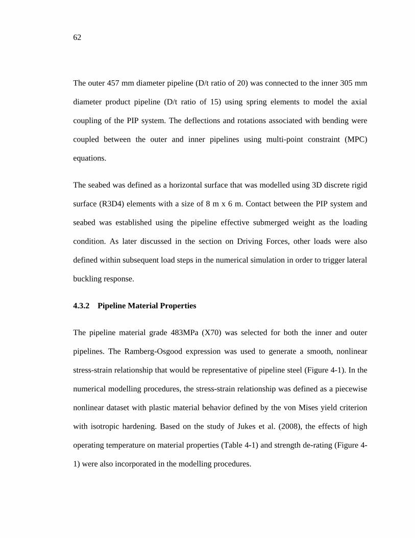
4.3 Numerical Modelling procedures ........................................................................ 60
4.3.1 Pipeline and Seabed Elements ..................................................................... 60
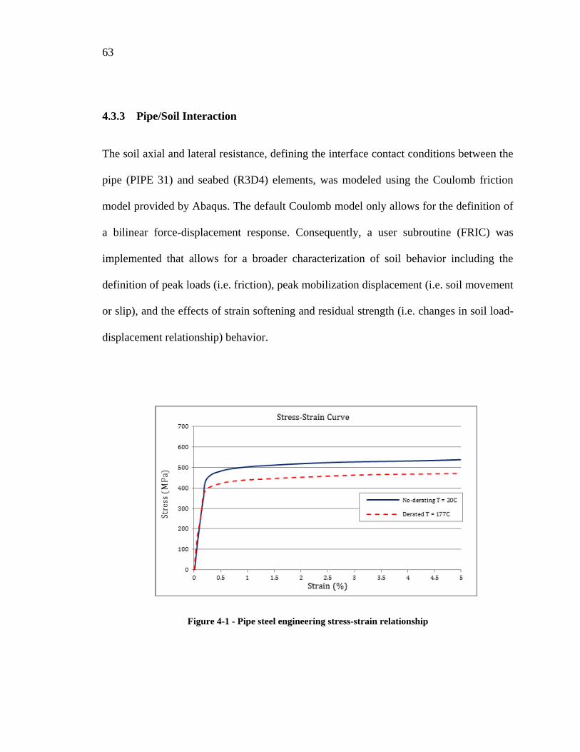
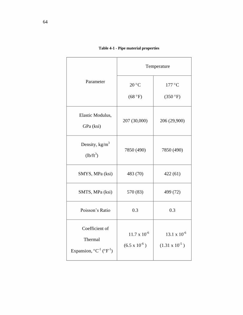
4.3.2 Pipeline Material Properties ......................................................................... 62
4.3.3 Pipe/Soil Interaction ..................................................................................... 63
4.3.4 Loading Conditions ...................................................................................... 67
4.3.5 Solution Algorithms ..................................................................................... 68
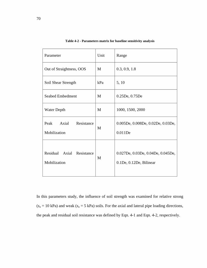
4.4 Parameter Study .................................................................................................. 69
4.5 Results and Discussion ........................................................................................ 72
4.5.1 Overview ...................................................................................................... 72
4.5.2 Peak Axial Mobilization Displacement ....................................................... 74
4.5.3 Residual Axial Mobilization Displacement ................................................. 76
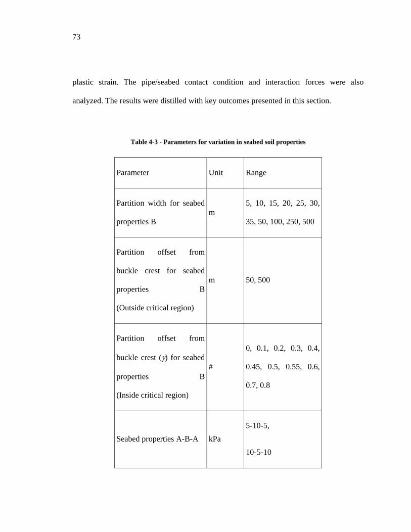
4.5.4 Non-Uniform Seabed Properties with Weak Soil Partition ......................... 80
4.5.5 Non-Uniform Seabed Properties with Strong Soil Partition ........................ 85
4.6 Conclusions ......................................................................................................... 90
4.7 Nomenclature ...................................................................................................... 93
4.8 Acknowledgments ............................................................................................... 95
4.9 References ........................................................................................................... 95
5 SUMMARY AND CONCLUSIONS ...................................................................... 100
5.1 Recommendations ............................................................................................. 104
6 REFERENCES ........................................................................................................ 106
List of Tables
Table 3-1 - Comparison of FE predictions with analytical solutions of Hobbs (1984) and
Lindholm (2007) ................................................................................................................ 38
Table 3-2 - Sensitivity analysis matrix .............................................................................. 40
Table 4-1 - Pipe material properties ................................................................................... 64
Table 4-2 - Parameters matrix for baseline sensitivity analysis ......................................... 70
Table 4-3 - Parameters for variation in seabed soil properties .......................................... 73
List of Figures
Figure 2-1 – First four mode shapes for lateral buckling (after. Hobbs. 1984) ................. 10
Figure 2-2 – Typical Snake-Lay Configuration (ref: Safebuck Design Guideline page C3)
............................................................................................................................................ 14
Figure 2-3 - Location of the pipe relative to trigger in a zero-bend method (a) touch down
(b) pullover (bending on the vertical pole) and (c) operating condition. (Courtesy: Peek
and Nils, 2009) ................................................................................................................... 17
Figure 2-4 - A Typical Pipe-in-Pipe Configuration (Courtesy: Jukes et al., 2008) .......... 20
Figure 2-5 - A Typical Load-displacement Soil Resistance Response .............................. 23
Figure 3-1 - First four mode shapes for lateral buckling (after Hobbs, 1984). ................. 30
Figure 3-2 - Load-displacement relationship during lateral buckling with OOS .............. 42
Figure 3-3 - Effective axial force due to lateral buckling with OOS ................................ 43
Figure 3-4 - Equivalent plastic strain due to lateral buckling with OOS ........................... 44
Figure 3-5 - Pipeline lateral buckled displacment profile with OOS ................................. 45
Figure 3-6 - Pipeline true axial strain due to lateral buckling with OOS ........................... 45
Figure 3-7 - Effective axial force due to lateral buckling with D/t ................................... 46
Figure 3-8 - Equivalent plastic strain due to lateral buckling with D/t .............................. 47
Figure 3-9 - True axial strain due to lateral buckling with D/t .......................................... 47
Figure 3-10 - Equivalent plastic strain due to lateral buckling with installation depth ..... 48
Figure 3-11 - Lateral displacement profile due to lateral buckling with operating
temperature ........................................................................................................................ 49
Figure 3-12 - True axial strain due to lateral buckling with operating temperature .......... 50
Figure 3-13 - Efective axial force due to lateral buckling with lateral friction coefficient51
Figure 3-14 - True axial strain due to lateral buckling with lateral friction coefficient .... 51
Figure 4-1 - Pipe steel engineering stress-strain relationship ............................................ 63
Figure 4-2 - Soil axial friction and mobilization distance relationship .............................. 67
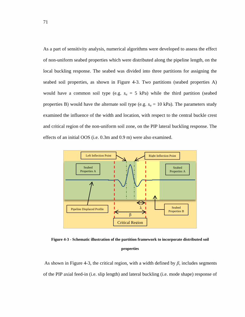
Figure 4-3 - Schematic illustration of the partition framework to incorporate distributed
soil properties ..................................................................................................................... 71
Figure 4-4 - Influence of elastic slip on lateral displacement profile for strong soil ......... 75
Figure 4-5 - Influence of elastic slip on lateral displacement profile for weak soil .......... 75
Figure 4-6 - Influence of soil residual mobilization distance on lateral buckle profile for
(a) strong soil with low OOS at intermediate water depth, (b) weak soil with low OOS at
shallow water depth and (c) weak soil with high OOS at deep water depth ...................... 78
Figure 4-7 - Influence of residual mobilization distance on PIP equivalent plastic strain
for weak soil with low OOS at shallow water depth ......................................................... 80
Figure 4-8 - Influence of the weak soil partition width for an OOS of (a) 0.3 m and (b) 0.9
m ........................................................................................................................................ 82
Figure 4-9 - Influence of the weak soil partition location for an OOS of (a) 0.3 m and (b)
0.9 m .................................................................................................................................. 84
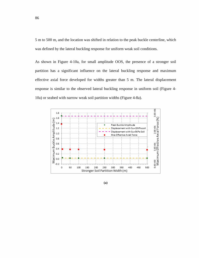
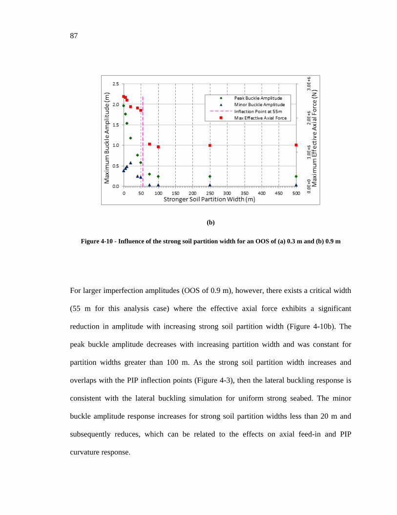
Figure 4-10 - Influence of the strong soil partition width for an OOS of (a) 0.3 m and (b)
0.9 m .................................................................................................................................. 87
Figure 4-11 - Influence of the strong soil partition location for an OOS of (a) 0.3 m and
(b) 0.9 m ............................................................................................................................. 89
1
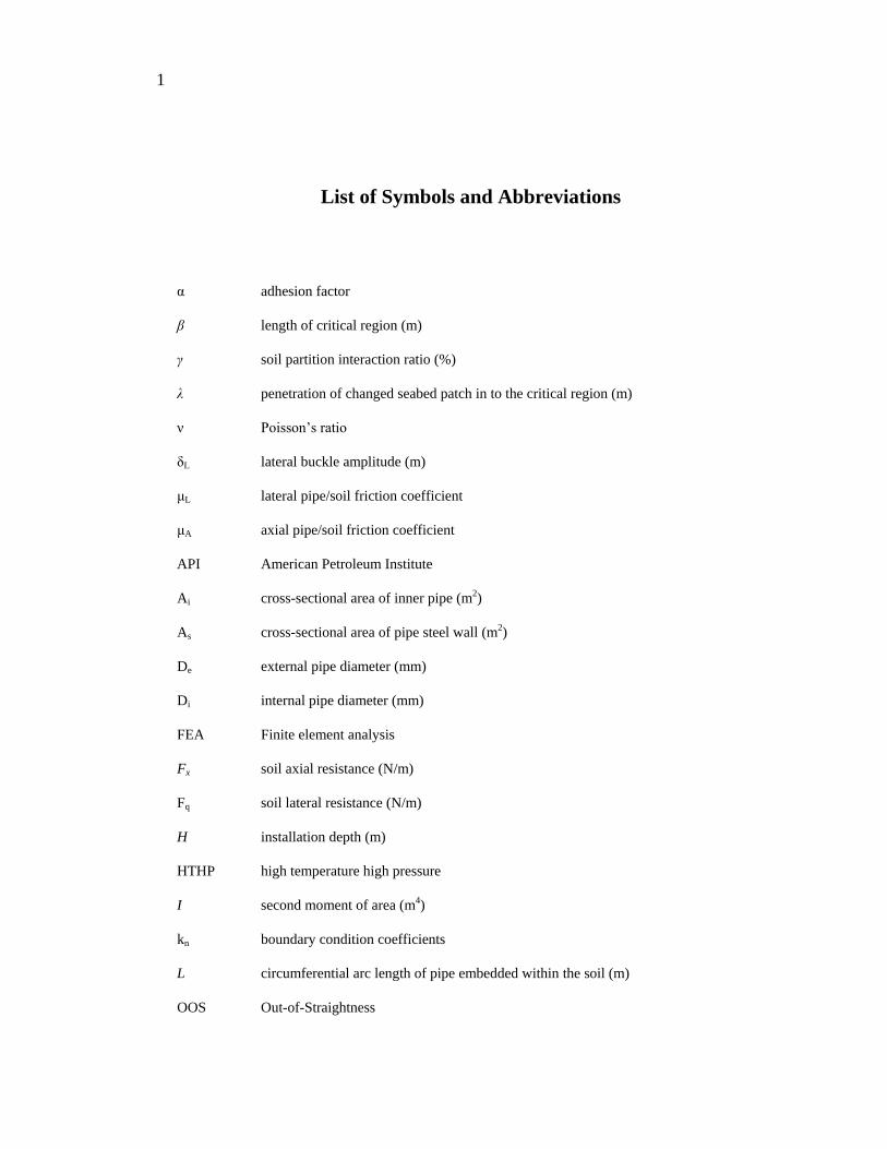
List of Symbols and Abbreviations
α adhesion factor
β length of critical region (m)
γ soil partition interaction ratio (%)
λ penetration of changed seabed patch in to the critical region (m)
ν Poisson’s ratio
δL lateral buckle amplitude (m)
μL lateral pipe/soil friction coefficient
μA axial pipe/soil friction coefficient
API American Petroleum Institute
Ai cross-sectional area of inner pipe (m2)
As cross-sectional area of pipe steel wall (m2)
De external pipe diameter (mm)
Di internal pipe diameter (mm)
FEA Finite element analysis
Fx soil axial resistance (N/m)
Fq soil lateral resistance (N/m)
H installation depth (m)
HTHP high temperature high pressure
I second moment of area (m4)
kn boundary condition coefficients
L circumferential arc length of pipe embedded within the soil (m)
OOS Out-of-Straightness
2
ΔPi internal pressure difference between the operational and as-laid conditions (MPa)
Pe external pressure (MPa)
Pi internal pressure (MPa)
PIP pipe-in-pipe
S effective axial force at the buckle (kN)
average soil undrained shear strength (kPa)
t pipe wall thickness (mm)
ΔT temperature differential between the between the operational and as-laid conditions (°C)
W pipeline submerged weight (N/m)
z pipeline embedment (m)
Su
3
1 INTRODUCTION
1.1 Overview
Offshore pipelines are a reliable, cost effective and safe mode of transporting
hydrocarbon products over long distances. In recent years, due to the global energy
demand, the oil and gas industry has expanded developments and operations into more
aggressive operating regimes associated with high temperature and high pressure (HTHP)
reservoirs, and harsh environmental conditions such as arctic and deep water regions.
Pipelines have a tendency to expand under operational loads. However, frictional forces
between the pipeline and surrounding seabed soil may restrict such movements. This
expansion is a result of an axial force, which may be large enough to initiate global Euler
buckling phenomenon (Kaye, 1996). For pipelines laid on the seabed or with partial
embedment, the potential for global instability mechanisms, such as lateral buckling
poses a major challenge in engineering design of deepwater pipelines (DNV RP-F110,
2007; Hobbs, 1984; Palmer et. al., 1990). Conventional approaches to stabilize this
pipeline movement through seabed intervention i.e. trenching, burial and rock dumping,
are impractical due to technical and economic constraints.
This study focuses on the mechanical integrity of pipelines in a post buckled condition
and the influence of various operational and geometric parameters on the lateral buckling
phenomena.
4
1.2 Scope and Objectives
The purpose of this study is to assess pipeline lateral buckling mechanisms through the
development of robust and accurate numerical modelling procedures. There are several
studies (Hobs, 1984; Palmer et al., 1990, Lindholm, 2007; Safebuck, 2005; Burton and
Carr, 2007; DNV-OS-F101) that have provided an insight on global buckling instability
and were used in this study to develop the calibrated finite element modelling procedures
for a single wall pipeline. Also, recent investigations by Jukes et al. (2008) provided the
basis to investigate lateral buckling behavior of Pipe-in-Pipe pipelines.
A high level of confidence must be achieved through calibration and verification of the
established algorithms with the data set and analytical equations available in the public
domain. Numerical models were developed for lateral buckling for a single wall pipe
using ABAQUS v 6.10 and were calibrated against analytical solutions. The approach for
calibrating the numerical models was twofold. Firstly, the effective axial force developed
in a perfectly straight pipe examined using ABAQUS was compared with analytical
solutions, and later a structural numerical model for a pipeline based on initial out of
straightness (OSS) was compared with the studies provided by Hobbs (1984) and
Lindholm (2007).
Once confidence in the finite element model was achieved, an analysis model matrix was
established to account for a range of influential parameters including initial out of
straightness profile, diameter to wall thickness ratio, installation depth, operating
5
temperature and coefficient of lateral friction between the pipeline and the seabed. The
influence of these variables was analyzed on the pipe buckled displacement profile,
effective axial force, true axial strain, plastic equivalent strain and pipe/seabed contact
shear force.
Based on the investigations of the sensitivity study, the developed finite element
algorithm was further refined to incorporate Pipe-in-Pipe (PIP) system, pipeline
penetration into the seabed, more realistic pipe/soil interaction (i.e. multi-linear soil
friction using user subroutine FRIC) and strength de-rating due to the effects of high
operating temperature on material properties.
The aim of this study is to draw guidelines to predict lateral movement and the displaced
profile of a buckled pipe under the influence of key parameters. The study also highlights
the importance of inflection points and a critical region surrounding the buckle crest at
pipe mid-length. Effects of a relatively strong seabed partition in overall softer seabed and
a relatively weak seabed partition in overall stronger seabed were also analyzed and
presented in this thesis.
A comprehensive numerical parameter investigation on the lateral buckling response of a
HTHP PIP pipeline was carried out. The parameters included pipe embedment, pipeline
initial out of straightness, soil shear strength, soil peak and residual forces and
displacements, variation in soil properties distributed along the pipeline route and external
pressure associated with the installation depth.
6
1.3 Thesis Layout
The thesis is divided into five chapters with chapter one and two focusing on scope of
work and literature review respectively. The literature review assessed the existing
database of physical modelling and numerical simulation, engineering practice and design
codes/standards for the effects of lateral buckling on pipeline performance. Global
buckling mechanism, buckle design strategies, effective axial force, pipe-in-pipe system
and pipe/soil interaction were examined. This task helped in identifying the existing
knowledge base, technology gaps and potential constraints that were used as foundation
for the study and framework to develop the numerical modelling procedures.
Chapters 3 and 4 are based on peer reviewed publications that discuss in detail the
different studies that were conducted to develop calibrated numerical modelling
procedures and post-buckled analysis for pipeline integrity assessment.
In depth calibration of the developed numerical modelling technique is discussed in
chapter 3 that focused on developing a calibrated single-walled pipeline model and
analyzed pipe/soil interaction and the global instability mechanism. A sensitivity analysis
was conducted and highlighted the significance of operational temperature, pipe diameter
to thickness ratio, internal and external pressure, and soil lateral friction characteristics on
the lateral buckling response.
The second part of the study (Chapter 4) focused on refining the developed calibrated
numerical tools to incorporate more realistic and complex non-linear behaviors, involving
7
pipe-in-pipe system, pipe strength de-rating due to the high operating temperatures and
enhanced pipe/soil interaction model to account for the effects of initial soil berm. The
influence of boundary conditions on the pipe mechanical response was also studied and
was found to be consistent with the initial study (Chapter 3). A sensitivity analysis matrix
was established to account for a range of key influential parameters. The aim of the
numerical parameter study was to assess lateral buckling response of a Pipe-in-Pipe (PIP)
system under the influence of varying seabed properties (i.e. non-uniform seabed),
pipeline penetration and elastic slip and peak resistance for axial friction.
Chapter 5 focuses on summarizing and concluding the research study. Significant results
generated throughout the study were compiled and the use of the developed numerical
algorithm is explained in this chapter. Recommendations were formulated and it was
stated that validation of the numerical tool through future physical testing will assist in
predicting more efficient and reliable pipe mechanical response.
8
2 LITERATURE REVIEW
2.1 General Overview
Pipelines are considered to be one of the most practical and cost effective methods for
transporting petroleum products since 1950’s. In the recent decades, the offshore oil and
gas industry has expanded operations into deeper and harsher operating regimes.
Consequently, subsea pipelines are increasingly being required to operate at high
temperature and high pressure operating conditions. Operation at such extreme conditions
increases the probability of pipeline failure and the severity of the damage is influenced
by a number of key factors including cyclic loads under frequent shutdown and startup
conditions, free spans, variable pipe/soil interaction over the length of the pipe, seabed
topology, axial and lateral friction load-displacement response, higher hydrostatic
pressure, long tie-backs, cold startups, etc. Due to an increase in structural integrity
concerns, different codes and standards have been introduced over a period of years.
Pipeline technology started to address the issue of in-service buckling in early eighties. A
series of studies conducted by Hobbs (1984) and Taylor and Ben Gan (1986) proposed
analytical tools to predict the occurrence and consequences of pipeline buckling. Over the
years, much work has been done to introduce a number of national standards to cover
issues that include pipeline design, manufacture, installation, construction, inspection and
repair (e.g. ASME B31.4, ASME B31.8, CAS-Z662, DNV1996, API 5L).
9
2.2 Global Buckling Mechanism
Subsea pipelines operating at pressures and temperatures higher than the ambient seabed
condition have a tendency to expand. This pipeline movement is restricted by external
reactions from structural supports and friction forces between the pipeline and the seabed.
Consequently, an axial force will be developed in the pipeline. This effective axial force
may be large enough to induce global (Euler) buckling (Kaye, 1996) and at some critical
value, the pipe may experience a snap through deformation. Axial friction forces may
lead to virtual anchor points where the axial friction force is equal to the effective axial
force.
DNV-RP-F110 indicates two design concepts to assure the integrity of pipelines,
susceptible to global buckling;
i. Restraining the pipeline and maintaining large compressive forces.
ii. Releasing the expansion forces and potentially causing global buckling with
resultant pipeline curvature.
Traditionally the petroleum industry has practiced to restrict the pipeline movement with
conventional design approaches to trench, bury, back fill and rock dump the pipeline.
Such techniques became technically impractical and expensive at deeper installation
depths and for high temperature and high pressure environments. Therefore, deep subsea
HTHP pipelines are laid on the seabed floor and may experience partial embedment under
their own weight. Pipelines laid on the seabed surface will exhibit lateral buckling over
10
vertical or upheaval buckling. Also, lateral buckling has less severe consequences than
upheaval buckling (Kaye, 1996) and it releases the high axial stress developed in the pipe
wall and will lower the effective axial force in the buckled region (Lindholm, 2007;
Safebuck, 2005; Burton and Carr, 2008).
The pipeline can exhibit either symmetric or asymmetric buckling modes, depending on
the initial geometric imperfection, lay tension etc. The line of symmetry is referred to an
axis drawn through the buckle crest and perpendicular to the original centerline of the
pipeline (Kaye, 1996). Experimental work performed by Hobbs (1984), has found that a
pipeline can buckle into different lateral mode shapes and mode 3 is the most stable
lateral buckle mode. Some common mode shapes are shown in Figure 2-1.
Figure 2-1 – First four mode shapes for lateral buckling (after. Hobbs. 1984)
Studies conducted by Burton et al. (2006, 2007, 2008) and Safebuck (2005) showed that
an uncontrolled lateral buckling event could be detrimental for the integrity of the
pipeline and may have serious consequences in the form of pipeline failure. These studies
11
have also shown that buckle mitigation techniques are not as effective as working with
the pipeline by controlling the formation of lateral buckles along the pipeline route,
leading towards buckle initiation strategies. Burton (2007) also concluded that controlled
lateral buckling may be the only economic solution as operating temperatures and
pressures are increased.
Maurizio et al. (1999) expressed the difficulties to meet the traditional stress based design
in scenarios where lateral buckling is anticipated and also such design might lead to thick-
walled pipes, to allow for large strains. However, as disused by Bruschi et al. (1993)
application of strain-based criteria depends on whether the condition is displacement or
load controlled. Therefore, strain or limit state based codes such as DNV-OS-F101 are
used to design the buckling characteristics of the pipeline (Sriskandarajah & Bedrossian,
2004).
2.3 Buckle Design Strategy
The number of buckles formed in a pipeline dictates the severity of the design problem,
the greater the number of buckles are, the lower the loading that develops in each buckle.
If the buckles are initiated at regular intervals along the pipeline, the loads are effectively
shared between the buckle sites. Uncontrolled lateral buckling will relieve the axial force
locally and a limited number of buckles will be formed which might not be enough for the
pipeline to operate safely.
12
Buckling has to be controlled to avoid excessive deformation at each buckle site by
limiting axial feed-in and to ensure regular buckles in each designed virtual anchor
spacing (VAS). Virtual anchor spacing is the distance between two adjacent virtual
anchor points. Also, short virtual anchor spacing will result in a lower probability of
buckle forming at the desired locations. Therefore, it is often a difficult design challenge
to select the most efficient spacing, maximizing both the number of buckles in the
pipeline and the probability of buckle forming at each designed site.
2.4 Buckle Initiation
Burton (2007) studied three key parameters governing the buckle initiation;
i. The effective compressive force in the pipeline (which is a function of axial
resistance.
ii. Out-of-straightness (OOS).
iii. Lateral breakout resistance.
Initial out-of-straightness could either be naturally induced or could also be introduced on
purpose in accordance with a buckle design strategy. Unintended geometric imperfections
arise from a number of sources and the most common causes of the imperfections are:
i. Uneven seabed.
ii. Pipeline lay route alignment.
iii. Barge motions during pipeline installation.
13
iv. Soil conditions.
v. Fishing gear interaction.
vi. Anchor dragging.
If no buckle initiation techniques are applied to generate buckles at the desired intervals,
the buckles will be induced at random locations and generally less frequently than if an
initiation strategy is utilized. Coupled with the uncertainty to produce acceptable results,
such random formation behavior is extremely challenging to predict. Therefore, buckle
initiation techniques must be adopted as a part of the design strategy, to increase the
probability of buckle forming at the anticipated locations.
Hobbs (1984), DNV RP-F110 and Kaye (1996) established that a lower effective axial
force is required to induce a buckling response for a pipeline with increased initial
geometric imperfection (out-of-straightness). Based on this principle, all of the buckle
initiation methods employ a relatively large initial out-of-straightness feature at the
intended locations. These engineered features are more severe than the inherent geometric
imperfections and therefore have a greater probability to develop lateral deformations.
Buckle initiation strategies have been extensively studied in the literature (Safebuck,
2005; Burton, 2007; Herlianto, 2001; Perinet D., 2006; Rathbone, 2008; Qiang Bai,
2014). Some of the methods which have been employed include;
i. Snake-lay.
ii. Vertical upset.
14
iii. Distributed buoyancy.
iv. Zero-radius bend (ZRB) method.
2.4.1 Snake-lay
Snake-lay installation is the most common buckle initiation method adopted to date by
the industry. In snake-lay method, the pipeline is laid on the seabed in a snake
configuration following a series of gentle curves. Figure 2-2 shows a typical snake-lay
pattern around a straight route centerline.
Figure 2-2 – Typical Snake-Lay Configuration (ref: Safebuck Design Guideline page C3)
The offset is defined as the amplitude (i.e. the distance from the crest of the snake to the
lay centerline), the pitch is the half wavelength and the bend radius is the radius of
curvature of the snake lay configuration.
15
The intention is that a buckle forms at each crown due to the horizontal OOS. The radius
is designed to act as a buckle initiator while the affinity for buckling decreases if the
radius of curvature is increased.
2.4.2 Vertical upset
Bai (2014) and Safebuck (2005) concluded that an initial vertical movement has a high
tendency to be converted into a lateral deformation. The vertical upset method is based on
this phenomenon. Normally two techniques are used to employ initial vertical out-of-
straightness:
i. Sleepers.
ii. Gravel dump berms.
Sleepers are essentially large diameter pipe sections prelaid on the seabed and
perpendicular to the longitudinal pipeline route alignment, to deliberately introduce a
vertical OOS at discrete sites along the pipeline. Friction between the sleeper and the pipe
can be minimized by coatings. Vertical imperfection also reduces uncertainties about the
pipe/soil interaction as the pipeline is suspended above the seabed on both sides of the
sleeper. In the gravel dump option, the sleeper is replaced by a gravel berm.
However, touch-down monitoring systems and sufficient accuracy is required to preinstall
the sleepers along the pipeline route and to lay the pipe over the center of the sleepers to
16
allow for the buckling event. Pipeline spans developed due to the vertical imperfections
are susceptible to vortex-induced vibrations and may be a fishing hazard as well.
2.4.3 Distributed Buoyancy
The distributed buoyancy method distributes buoyancy modules at the intended buckle
initiation sites. The effective submerged weight is then a small fraction of the normal
submerged weight at the buoyant locations. The pipeline tends to form vertical
imperfections during the laying process and a very low submerged weight reduces the
lateral friction restrain.
2.4.4 Zero-Radius Bend Method
The zero-radius bend method is a fairly new and reliable technique to trigger a lateral
buckle and is capable of initiating lateral buckles at low axial compressive force. This
method is studied in detail by Peek and Kristiansen (2009). The approach includes both
vertical and horizontal imperfections and involves a vertical pole and a slanting surface,
the pipeline falls off the trigger during lateral buckling, eliminating the spans thereby
eliminating potential fatigue from vortex induced vibrations. The pipeline is laid on
preinstalled triggers and is bent laterally on the vertical pole. This method is more
efficient but the installation process needs to be monitored using transponders and
remotely operated vehicles.
17
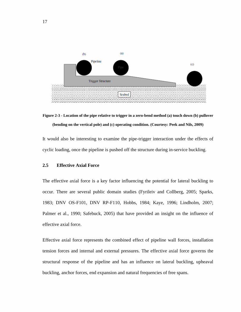
Figure 2-3 - Location of the pipe relative to trigger in a zero-bend method (a) touch down (b) pullover
(bending on the vertical pole) and (c) operating condition. (Courtesy: Peek and Nils, 2009)
It would also be interesting to examine the pipe-trigger interaction under the effects of
cyclic loading, once the pipeline is pushed off the structure during in-service buckling.
2.5 Effective Axial Force
The effective axial force is a key factor influencing the potential for lateral buckling to
occur. There are several public domain studies (Fyrileiv and Collberg, 2005; Sparks,
1983; DNV OS-F101, DNV RP-F110, Hobbs, 1984; Kaye, 1996; Lindholm, 2007;
Palmer et al., 1990; Safebuck, 2005) that have provided an insight on the influence of
effective axial force.
Effective axial force represents the combined effect of pipeline wall forces, installation
tension forces and internal and external pressures. The effective axial force governs the
structural response of the pipeline and has an influence on lateral buckling, upheaval
buckling, anchor forces, end expansion and natural frequencies of free spans.
18
For a fully restrained pipeline under the load effects from operating conditions, the far
field effective axial force can be defined as (DNV OS-F101; Sparks, 1983; Fyrileiv and
Collberg, 2005):
( ) – Eqn. 2.1
Eqn. 2.1 suggests that the axial force will be more compressive if internal pressure is
increased. Similarly, an increase in the external pressure will stabilize the buckle.
An analytical solution developed by Hobbs (1984) and discussed by Kaye (1996), Palmer
(1990) and Safebuck (2005) provides a basis to predict the critical buckling load. As
explained by Herlianto (2011), Hobbs used the technical approach based on a force-
displacement relationship and compatibility in the post-buckle state. The analytical
solution relates the buckle wavelength with the effective force through the expressions:
Eqn. 2.2
[√
( ) ] Eqn. 2.3
Eqn. 2.4
[ ( )
( )
] ⁄
Eqn. 2.5
19
Lindholm (2007) showed that if only mode 3 deformation waveforms are considered, the
Eqn. 2.2 and Eqn. 2.4 can be combined to establish a relationship between the buckle
crown displacement and the effective axial force in the buckle. The resulting equation is
given as:
√
Eqn. 2.6
where So is the effective axial force required to initiate lateral sliding in a pipe with an
initial lateral imperfection of .
2.6 Pipe-in-Pipe System
Pipe-in-pipe (PIP) systems have been developed essentially to address the engineering
requirements with regards to flow assurance. One of the major issues during HTHP
pipeline operation is the loss of heat energy through pipe wall. As a result, critical wax
allowable temperature (WAT) may be reached resulting in the formation of asphaltenes
and ultimately blocking the pipeline. A PIP systems provides a solution to mitigate
formation of wax, asphaltenes and hydrates during both steady-state operations and
transient cool-down and re-start conditions.
PIP flowlines provides a low ‘Overall Heat Transfer Coefficient’ (OHTC) and are
frequently used where a high thermal performance (i.e. OHTC < 1W/m2K) is required
(Jukes et al., 2008). PIP systems have been studied in detail by Safebuck (2005), DNV
20
RP-F110, Jukes et al. (2008) and Zhao et al. (2007) and Figure 2-3 shows a typical pipe-
in-pipe system configuration.
Figure 2-4 - A Typical Pipe-in-Pipe Configuration
(Courtesy: Jukes et al., 2008)
A PIP system consists of an inner carrier pipe, an outer jacket pipe and the annulus in
between is filled with dry insulation material like mineral wool, polyurethane foam,
aerogel, granular or microscopic materials or ceramics. PIP systems are generally
categorized in three types of systems:
i. Fully bonded.
ii. Complaint.
iii. Non-complaint.
21
In a fully bonded PIP system, a continuous shear transfer between the inner flowline and
the outer pipe is delivered through the annulus insulation. A concentric bending is
enforced for both the inner and the outer pipes. The system bends as a composite with
equal curvature in both pipes.
The compliant or regular bulkhead system connects the two pipes through frequently
spaced structural connectors (bulkheads), these connectors are also known as tulips or
donut plates. The axial strain in the two pipes is not necessarily equal, specifically at the
buckle crown, however as the distance between the bulkhead connections become shorter
then the bending curvatures are similar.
Non-compliant or unconnected system allows some degree of axial movement between
the two pipes and the interaction between the carrier pipe and the jacket pipe is frictional.
The only structural connection (structural bulkhead) is at the end of the pipeline, or
placed at significant spacing. However, centralizers or spacers may be used to keep the
two pipes concentric.
2.7 Pipe/soil Interaction
An understanding of pipe/soil interaction is essential to determine the buckling
phenomenon, and both axial and lateral frictional forces play an important role. It is a
very challenging task to predict the interaction behavior due to a number of complexities
and large uncertainties associated with the pipeline geotechnics. The pipe/soil load-
displacement response is estimated according to either total stress or effective stress soil
22
models that consider drained or undrained loading conditions. Cathie et al. (2005), ALA
(2005), Wantland (1979), Phillips et al. (2004), Pike et al. (2012), Dendani and Jaeck
(2008), DNV RP-F110, Safebuck (2005) have conducted studies on the key factors
influencing pipeline/seabed interaction. These factors include pipe diameter, embedment,
soil type and soil strength.
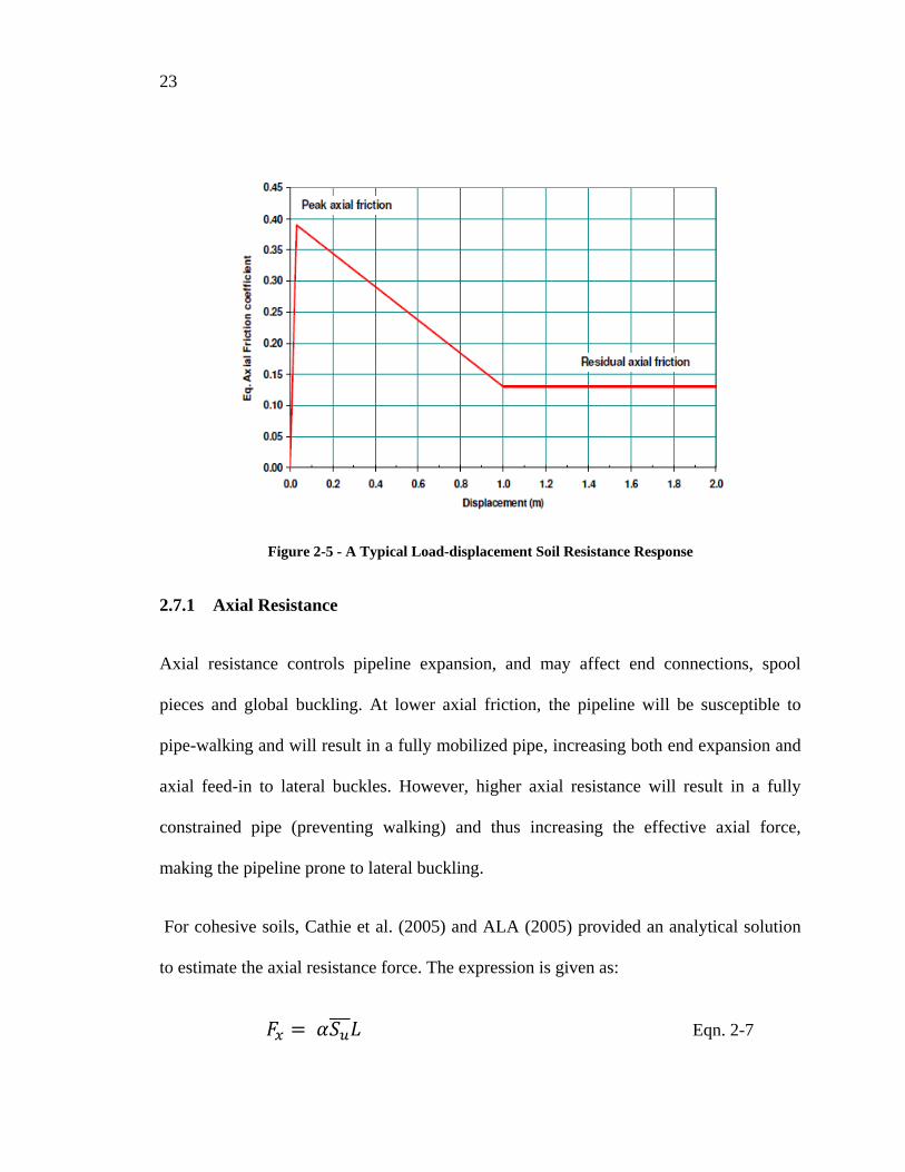
As-laid embedment restricts the initial movement of the pipeline. A significant maximum
friction force can occur at small mobilization displacements upon the first load scenario
or after a long period of pipe settlement. However, during subsequent loading with not
enough time for the pipeline to settle in the seabed again, this peak response might not be
observed. The mobilization displacement required to reach the peak resistance is also
known as elastic slip. Once the peak resistance is reached and the pipe over rides the
initial embedment, both axial and lateral friction will decrease to a steady residual
friction. One of the reasons for this behavior in load-displacement response could be that
a gap is formed between the pipeline and the soil wedge. Seabed lateral resistance may
increase after the lateral residual resistance is mobilized due to the formation of new
berms after the pipe has slipped significantly relative to the seabed. New berms are
created if the pipeline scrapes the seabed and pushes a soil mass during lateral
deformations.
23
Figure 2-5 - A Typical Load-displacement Soil Resistance Response
2.7.1 Axial Resistance
Axial resistance controls pipeline expansion, and may affect end connections, spool
pieces and global buckling. At lower axial friction, the pipeline will be susceptible to
pipe-walking and will result in a fully mobilized pipe, increasing both end expansion and
axial feed-in to lateral buckles. However, higher axial resistance will result in a fully
constrained pipe (preventing walking) and thus increasing the effective axial force,
making the pipeline prone to lateral buckling.
For cohesive soils, Cathie et al. (2005) and ALA (2005) provided an analytical solution
to estimate the axial resistance force. The expression is given as:
Eqn. 2-7
24
Where, is the adhesion factor and L is the pipeline arc length embedded in the soil.
The above expression suggests that the mobilized axial soil friction response is
proportional to the soil undrained shear strength, pipe/soil contact area and interface
effects.
Based on pipe/soil interaction tests conducted on natural clay, Dendani and Jaeck (2008)
estimated the value of adhesion factors of 0.7 and 0.35 for the peak and residual axial
resistance, respectively. For shallowly embedded pipes, the axial peak mobilization
distance was defined as 0.3% to 0.8% of the outside pipe diameter. Elastic slip
displacement required to mobilize axial breakout resistance is directly proportional to the
pipeline penetration into the seabed. Larger mobilization distance of 2% to 3% of the
outside diameter was observed for pipe penetrations exceeding 50% of the pipe diameter.
Residual axial friction was reached within a displacement range of 1.35 times to
approximately 1.5 times the peak mobilization distance.
2.7.2 Lateral Resistance
Soil lateral resistance influences the pipe lateral displacement and governs the level of
pipe curvature and pipe bending stress. Reducing the lateral friction will reduce the
severity of the buckle and therefore, allow an increase in the virtual anchor spacing
without compromising the integrity of the pipeline. Several methods can be adopted to
reduce the lateral resistance, including seabed preparation through gravel dumping,
25
reducing effective submerged weight by reducing weight coating, increasing pipeline
buoyancy or to use pipeline sleepers.
Cathie et al. (2005) and Dendani (2008) have assessed the three different procedures to
estimate the lateral resistance load-displacement response:
i. Single friction factor.
ii. Two component model.
iii. Plasticity model.
Single friction factor approach relates the lateral resistance with the pipeline submerged
weight and the soil type. This is a very basic approach and does not incorporate pipeline
embedment. As studies from Wanger et al. (1987) Lieng et al. (1988) and Verley and
Lund (1995) showed, the two component model considers a sliding friction component
and a lateral passive pressure component. The plasticity model developed by Zhang et al.
(1999, 2002) defines the movement direction during yield, incorporating yield surface,
strain-hardening expression, elastic behavior inside yield surface and a flow rule.
Dendani and Jaeck (2008) also estimated the lateral resistance force and is expressed as:
Eqn. 2-8
where c is an empirical coefficient and a value of 2.3 was reported for a pipe penetration
greater than 20% of the pipe outer diameter.
26
2.8 User Subroutine FRIC
For surficial and partially embedded pipelines, the simple Coulomb friction model does
not provide a detailed estimation of the complex behaviors, occurring during pipeline-soil
interaction. The basic Coulomb friction model provides a bilinear elastic-perfectly plastic
resistance response and was studied in the initial part of this research program.
The peak load, soil failure mechanism and the soil yield displacement involves the pipe
embedment ratio. Limiting friction (i.e. sliding mechanism) governs the failure
mechanism for surface laid pipelines while a passive wedge failure mechanism is
associated with deeper pipe penetration up to embedment ratios of 2.5 (Wantland et al.,
1979). Even small axial misalignments or pipe asperity can affect the axial and lateral soil
resistance (Philips et al., 2004; Pike et al., 2012).
User subroutines are capable of accounting for more complex soil force-displacement
behavior including brittle breakout behavior and berm development during pipe/soil
interaction events (Burton et al., 2007). User subroutine FRIC was also implemented to
model a non-linear force displacement response, which incorporated mobilization of soil
forces and displacements that can account for as-laid embedment, berm development,
breakout and residual strength conditions for surficial and partially embedded pipelines.
27
3 LATERAL BUCKLING RESPONSE OF SUBSEA HTHP
PIPELINES USING FINITE ELEMENT METHODS
This paper has been published in the proceedings of 32nd International Conference on Ocean, Offshore and Arctic Engineering, Nantes,
France, 2013. As the principal investigator and first author, the author of the thesis was responsible for conducting the numerical
investigation, analyzing the data, and reporting it inside this paper. The second author, Dr. Shawn Kenny, was responsible for
supervision of the investigation and guidance on data analysis.
Authors: Muhammad Masood ul Haq and Shawn Kenny
3.1 Abstract
Subsea pipelines are subject to load effects from external hydrostatic pressure, internal
pressure, operating temperature, ambient temperature and external reactions (e.g. seabed,
structural support). These parameters influence the effective axial force that governs the
pipeline global buckling response. Other factors, including installation stress, seabed
slope, soil type, and embedment depth, can influence the pipe effective force.
Pipelines laid on the seabed surface or with limited embedment may experience lateral
buckling. The resultant mode response is a complex function related to the spatial
variation in these parameters and kinematic boundary conditions.
In this paper, results from a parameter study, using calibrated numerical modelling
procedures, on lateral buckling of subsea pipelines are presented. The parameters
included pipe diameter to wall thickness (D/t) ratio, pipe out of straightness (OOS),
operating temperature and internal pressure, external pressure associated with the
installation depth, and seabed lateral and axial friction properties.
28
3.2 Introduction
In recent years, the oil and gas industry has expanded developments and operations into
deeper waters with harsher operating conditions. Pipelines are one of the most efficient
and economical solutions for transporting oil and gas. Pipelines may expand due to
operational loading conditions and may be restrained by the surrounding seabed soil or
structural supports due to frictional forces. The axial force that develops may be large
enough to induce Euler (global) buckling of the pipeline (Kaye, 1996).
Subsea pipelines are increasingly being designed to operate at ultra-deep water depths and
at much higher temperatures and pressures (HTHP). Exposure to such high operating
parameters increases the natural tendency of a pipeline to relieve the resulting high axial
stress in pipe-wall through buckling. For deep water and ultra-deep water environments,
restraining pipeline movement against higher operating temperatures at deeper water
depths will impact cost and technical risk with respect to seabed interventions where
conventional design approaches to trench and bury the HTHP pipeline become
impractical.
Consequently, the pipelines are laid on the seabed surface that may result in lateral pipe
buckling. Under such conditions it is more favorable to work with the buckle formation
rather than prevent the global mechanisms form occurring. Controlled lateral buckling
(e.g. initial OOS through snake lay installation, seabed supports) is an efficient solution
for the relief of axial compression. Lateral buckling may provide the only economical
29
solution as the operating conditions (i.e. temperature and pressures) are increased (Bruton
and Carr, 2007).
The initial OOS introduces a global imperfection mode shape in the pipeline that has a
significant effect on lateral buckling response due to the influence on the effective axial
force required to trigger lateral buckling. The pipeline route alignment, installation
process, seabed topography and soil conditions will generally establish the pipe initial
OOS. External interference, such as trawl gear or anchor dragging events, may also
impose lateral imperfections.
The pipeline can exhibit either symmetric or asymmetric buckling modes. The line of
symmetry is referred to an axis drawn through the center of the buckle and perpendicular
to the original centerline of the pipeline (Kaye, 1996). Experimental work performed by
Hobbs (1984), has found that pipeline can buckle into different lateral mode shapes.
Some common mode shapes are shown in Figure 3-1.
30
Figure 3-1 - First four mode shapes for lateral buckling
(after Hobbs, 1984).
This paper presents the results from a calibration study to develop numerical modelling
procedure to predict the lateral buckling response of single wall steel pipeline. A
parameter study was conducted where the significance of pipe D/t and OOS, operating
temperature and internal pressure, external pressure associated with the installation depth,
and seabed lateral and axial friction properties was examined. The predicted pipe
displacement, strain, and effective axial forces and seabed contact forces are examined.
The current paper will provide the foundation for future studies to establish engineering
guidance on pipe lateral buckling with respect to additional parameters including pipe
configuration (e.g. pipe-in-pipe), and seabed characteristics (e.g. slope, bathymetry,
vertical profile, spatial variation in frictional properties).
31
3.3 Nomenclature
δL lateral buckle amplitude (m)
ν Poisson’s ratio
μL lateral pipe/soil friction coefficient
μA axial pipe/soil friction coefficient
λ buckle wavelength estimate (m)
Ai cross-sectional area of inner pipe (m2)
As cross-sectional area of pipe steel wall (m2)
De external pipe diameter (mm)
Di internal pipe diameter (mm)
E modulus of elasticity (GPa)
H installation residual lay tension (m)
I second moment of area (m4)
kn boundary condition coefficients
L pipeline length (m)
OOS Out-of-Straightness
ΔPi internal pressure difference between the operational and as-laid conditions (MPa)
Pe external pressure (MPa)
Pi internal pressure (MPa)
q submerged weight (N/m)
SMYS specified minimum yield strength (MPa)
t pipe wall thickness (mm)
ΔT temperature differential between the between the operational and as-laid conditions (i.e.
external ambient seawater temperature) (°C)
Ti initial temperature (°C)
32
To operating temperature (°C)
S effective axial force at the buckle (kN)
So far field effective axial force (kN)
Z installation depth (m)
3.4 Numerical Modelling procedures
3.4.1 Pipeline and Seabed Elements
The pipe was modeled using the 2-node, linear Timoshenko beam element (PIPE31),
which allows for transverse shear deformations. This element is well suited to model
simulations including pipe laying and pipe/seabed contact simulations (Abaqus Analysis
User Manual). A pipe element length of 0.6 m, extending 100 m length on each side of
the buckle crest at pipe mid-length, was employed in order to capture the lateral buckling
mode. A pipe element length of 4 m was used outside this zone to capture the virtual
anchor and end boundary conditions. A pipeline length of 2000 m was sufficient to
capture the virtual anchor. This mesh topology was consistent with previous studies
(Safebuck, 2006). An initial pipeline out of straightness (OOS) was also defined to
promote lateral buckling response.
The pipe elastic material behavior was modeled with a Young’s modulus of 207 GPa,
Poisson’s ratio of 0.3, thermal expansion coefficient of 1.17 x 10⁻⁵ and density of 7850
kg/m3. A Grade 450 (X65) pipe material was selected where the stress-strain relationship
33
was defined by the Ramberg-Osgood expression through piecewise approximation.
Isotropic hardening with the von Mises yield criterion was used to define the constitutive
behavior. In this study, the effects of operating temperature on strength de-rating were not
examined as the study was focused on establishing the response for fixed parameters. A
future study will investigate the effects of a spatial variation on the lateral buckling
response for comparison with this baseline study.
The seabed was defined as a horizontal rigid surface that was modeled as a 3D discrete
rigid surface using R3D4 elements with a mesh size of 8 x 6 m. The pipe/seabed interface
friction was based on the Coulomb friction model with anisotropic properties for the axial
and lateral pipe axes. Based on the literature review, the best estimate defining the pipe
breakout axial and lateral friction coefficients was 0.6 and 0.8, respectively (Rong et al.,
2009). The breakout friction factors define a bilinear response. The axial friction
coefficient influences pipe axial forces and feed-in response during the buckling event,
whereas the lateral friction coefficient affects bending severity (Safebuck, 2006).
3.4.2 Driving Forces
The effective axial force is a key factor influencing the potential for lateral buckling to
occur (Fyrileiv and Collberg, 2005; Sparks, 1983). Buckle initiation is dependent on the
effective axial compressive force, pipe OOS and lateral breakout resistance due to
pipeline/soil interaction (Burton. et al. 2008; Safebuck, 2005). For a fully restrained
pipeline, the far field effective axial force can be defined as (DNV OS-F101):
34
Eqn. 3-1
The ambient seawater temperature (5 °C) and distributed submerged weight loading
condition was applied in the initial load step with the pipeline end boundary conditions
defined as encastre. The seawater density was 1025 kg/m3 and the pipeline density was
7850 kg/m3. In a second load step, the external and internal pressure loads and operating
temperature were defined. The external hydrostatic pressure was based on the water depth
(500 m, 1000 m and 2000 m). The internal pressure was held constant and defined as the
pressure required to produce a hoop stress equal to 80% SMYS. A range of operating
temperatures were examined that included 50 °C, 100 °C.
3.4.3 Solution Algorithms
The lateral buckling event involves complex, nonlinear mechanics due to the inherent
instability associated with the transition from equilibrium configurations through large
deformations, material response and pipe/seabed contact. The use of modified Riks
formulation is required for the solution to these equilibrium equations. As the internal
pressure and temperature differential provide the driving force, the pipeline load and
displacement response are unknown quantities that are determined through the
simultaneous solution (Abaqus Analysis User Manual; Chee, 2011; Zhao. et al. 2007).
So = H - DPiAi 1- 2n( )- AsEa DT
35
3.5 Calibration Study
3.5.1 Overview
The numerical modelling procedures developed in this study were based on investigations
and data available in the public domain (Bruton and Carr, 2007; DNV-OS-F101; Hobbs,
1984; Lindholm, 2007; Safebuck 2005). The Safebuck joint industry project (JIP) was
initiated to address the need for a robust lateral buckling design solution and improved
understanding on the related phenomenon of pipeline walking (Bruton and Carr, 2007).
The motivation of the current study is to develop structural finite element modelling
procedures to examine the lateral buckling response of HTHP pipelines with results that
are consistent with current state-of-practice over a range of practical design parameters.
3.5.2 Methodology
The approach for calibrating the numerical modelling procedures was twofold, whereby
(1) the effective axial force developed in a perfectly straight pipeline was examined using
Abaqus and compared with Eqn. 3-1, and (2) the Abauqs FE solution was compared with
the studies by Hobbs (1984) and Lindholm (2007) for a pipeline with an initial OOS
condition.
A series of case studies were solved using Abaqus FE and compared with the theoretical
solution for the effective axial force of a straight pipeline. The FE predictions were less
then 5% difference from the analytical solutions.
36
For HTHP pipelines with an initial OOS, the effective axial force is a key factor
influencing the lateral buckling response. Unlike upheaval buckling, the lateral buckling
response may evolve into higher order mode shapes (Figure 3-1) that define the post-
buckled configuration (Palmer et al., 1990; Hobbs, 1984; Zhao et al., 2007). The critical
buckling load or effective axial force varies for each mode shape. Furthermore, based on
energy considerations, mode 1 buckled shapes may evolve into higher order mode shapes
with lower potential energy states.
An analytical solution developed by Hobbs (1984) provides a basis to predict the critical
buckling load. The technical approach is based on force displacement relationship and
compatibility in the post-buckle configuration (Herlianto, 2011). The analytical solution
relates the buckle wavelength with the effective force through the expressions:
S = k1
EI
l 2 Eqn. 3-2
So = S + k3mAl1+ k2AEmLql
5
EI( )2
-1é
ë
êê
ù
û
úú
Eqn. 3-3
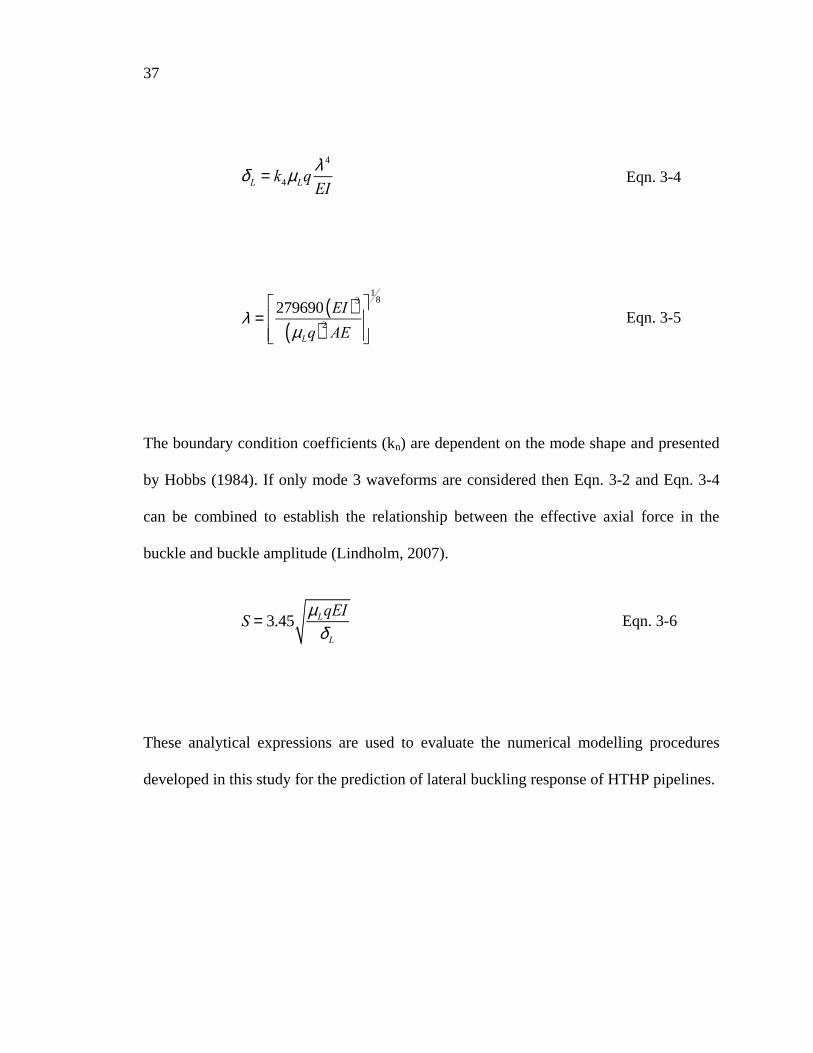
37
d L = k4mLql 4
EI Eqn. 3-4
l =279690 EI( )
3
mLq( )2AE
é
ë
êê
ù
û
úú
18
Eqn. 3-5
The boundary condition coefficients (kn) are dependent on the mode shape and presented
by Hobbs (1984). If only mode 3 waveforms are considered then Eqn. 3-2 and Eqn. 3-4
can be combined to establish the relationship between the effective axial force in the
buckle and buckle amplitude (Lindholm, 2007).
S = 3.45mLqEI
d L Eqn. 3-6
These analytical expressions are used to evaluate the numerical modelling procedures
developed in this study for the prediction of lateral buckling response of HTHP pipelines.
38
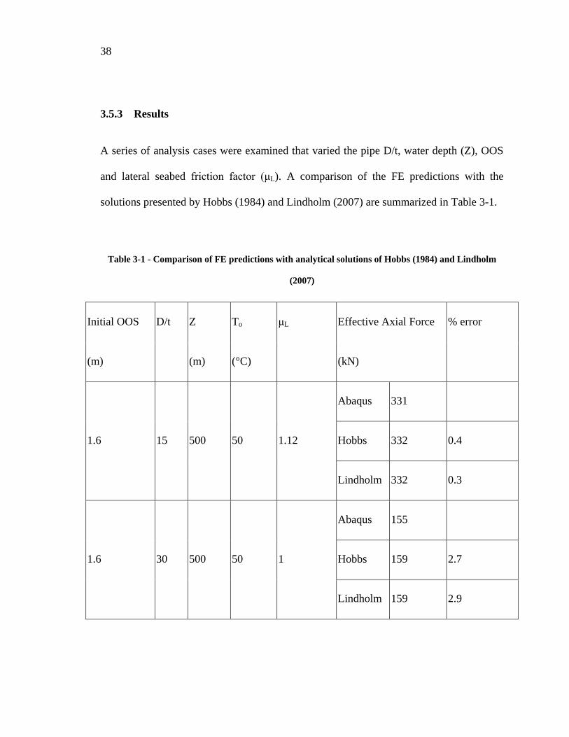
3.5.3 Results
A series of analysis cases were examined that varied the pipe D/t, water depth (Z), OOS
and lateral seabed friction factor (μL). A comparison of the FE predictions with the
solutions presented by Hobbs (1984) and Lindholm (2007) are summarized in Table 3-1.
Table 3-1 - Comparison of FE predictions with analytical solutions of Hobbs (1984) and Lindholm
(2007)
Initial OOS D/t Z To μL Effective Axial Force % error
(m) (m) (°C) (kN)
1.6 15 500 50 1.12
Abaqus 331
Hobbs 332 0.4
Lindholm 332 0.3
1.6 30 500 50 1
Abaqus 155
Hobbs 159 2.7
Lindholm 159 2.9
39
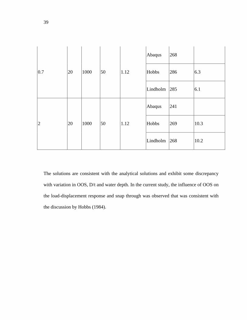
0.7 20 1000 50 1.12
Abaqus 268
Hobbs 286 6.3
Lindholm 285 6.1
2 20 1000 50 1.12
Abaqus 241
Hobbs 269 10.3
Lindholm 268 10.2
The solutions are consistent with the analytical solutions and exhibit some discrepancy
with variation in OOS, D/t and water depth. In the current study, the influence of OOS on
the load-displacement response and snap through was observed that was consistent with
the discussion by Hobbs (1984).
40
3.6 Parameter Study
3.6.1 Overview
Having established confidence in the numerical modelling procedures, a parameter matrix
was defined to conduct a sensitivity analysis (Table 3-2). The effects of pipe D/t,
operating temperature, installation depth, OOS and pipe/seabed interface friction on the
lateral buckling response were examined.
For the matrix scenarios including D/t of 30 and water depth of 2000 m, the pipe did not
meet the collapsepressure design check and were thus not included in the senstivity
analysis. A total of 216 simulations were performed with the remaining possible
permutations presented in the sensitivity matrix (Table 3-2).
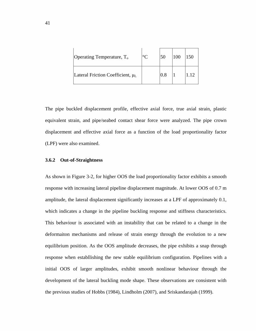
Table 3-2 - Sensitivity analysis matrix
Parameter Unit Range
Out of Straightness, OOS m 0.7 1.6 2
D/t
15 20 30
Installation Depth, Z m 500 1000 2000
41
Operating Temperature, To °C 50 100 150
Lateral Friction Coefficient, μL
0.8 1 1.12
The pipe buckled displacement profile, effective axial force, true axial strain, plastic
equivalent strain, and pipe/seabed contact shear force were analyzed. The pipe crown
displacement and effective axial force as a function of the load proportionality factor
(LPF) were also examined.
3.6.2 Out-of-Straightness
As shown in Figure 3-2, for higher OOS the load proportionality factor exhibits a smooth
response with increasing lateral pipeline displacement magnitude. At lower OOS of 0.7 m
amplitude, the lateral displacement significantly increases at a LPF of approximately 0.1,
which indicates a change in the pipeline buckling response and stiffness characteristics.
This behaviour is associated with an instability that can be related to a change in the
deformaiton mechanisms and release of strain energy through the evolution to a new
equilibrium position. As the OOS amplitude decreases, the pipe exhibits a snap through
response when establlishing the new stable equilibrium configuration. Pipelines with a
initial OOS of larger amplitudes, exhibit smooth nonlinear behaviour through the
development of the lateral buckling mode shape. These observations are consistent with
the previous studies of Hobbs (1984), Lindholm (2007), and Sriskandarajah (1999).
42
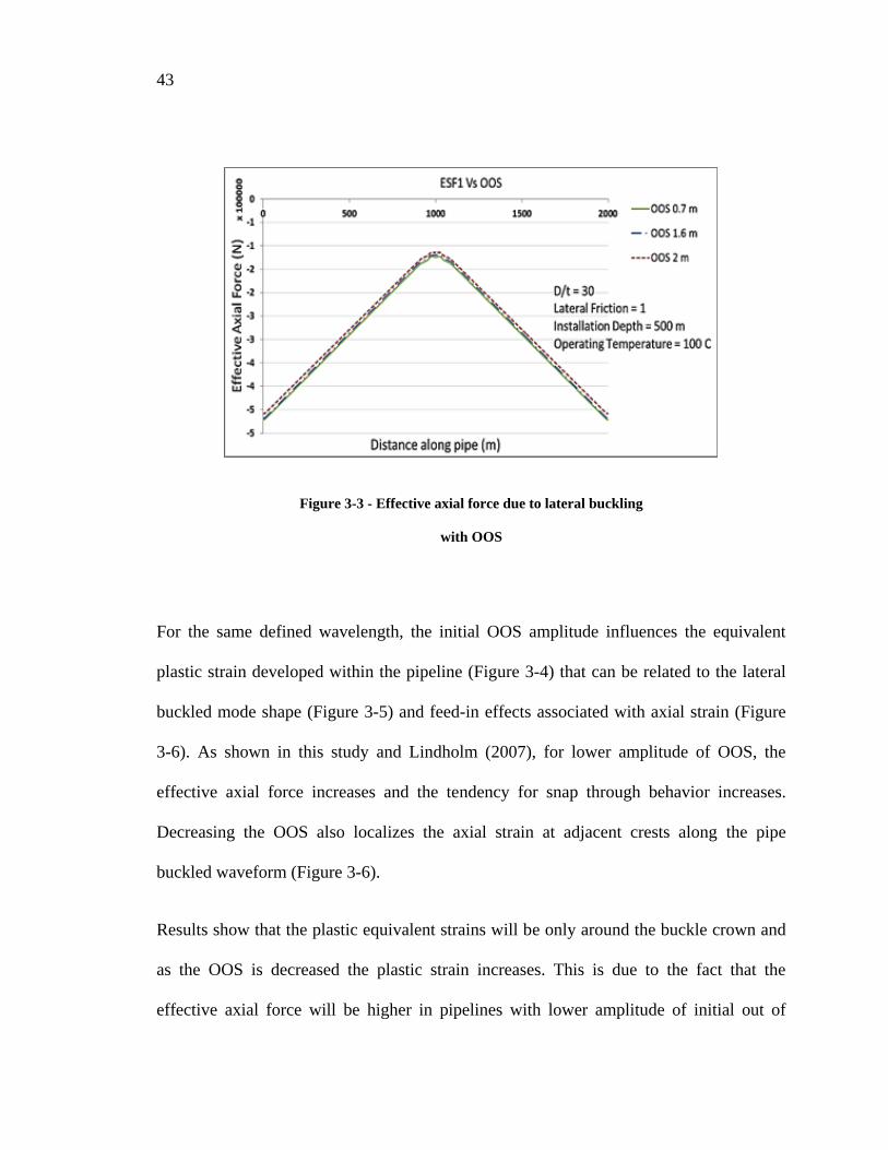
Although a weak relationship was observed, the effective axial force magnitude was
inversely proportional to the initial OOS amplitude (Figure 3-3). The compressive
effective axial force increases from the peak buckle toward the anchored ends of the
pipeline, which is also consistent with the studies conducted by Safebuck (2005). The
buckle amplitude is also inversely proportional to the required effective axial force to
initiate instability (Eqn.3-6).
Figure 3-2 - Load-displacement relationship during lateral buckling with OOS
43
Figure 3-3 - Effective axial force due to lateral buckling
with OOS
For the same defined wavelength, the initial OOS amplitude influences the equivalent
plastic strain developed within the pipeline (Figure 3-4) that can be related to the lateral
buckled mode shape (Figure 3-5) and feed-in effects associated with axial strain (Figure
3-6). As shown in this study and Lindholm (2007), for lower amplitude of OOS, the
effective axial force increases and the tendency for snap through behavior increases.
Decreasing the OOS also localizes the axial strain at adjacent crests along the pipe
buckled waveform (Figure 3-6).
Results show that the plastic equivalent strains will be only around the buckle crown and
as the OOS is decreased the plastic strain increases. This is due to the fact that the
effective axial force will be higher in pipelines with lower amplitude of initial out of
44
straightness. The same effect can be shown in Figure 3-4 which presents the generated
results for equivalent plastic strain while Figure 3-6 illustrates axial strains. It was also
observed that axial strain is higher at the crest of adjacent smaller buckles for lower OOS
amplitude.
Figure 3-4 - Equivalent plastic strain due to lateral buckling with OOS
45
Figure 3-5 - Pipeline lateral buckled displacment profile with OOS
Figure 3-6 - Pipeline true axial strain due to lateral buckling with OOS
46
3.6.3 Pipeline D/t Ratio
As defined by Eqn. 3-1, the effective axial force increases with increasing wall thickness,
which is shown in Figure 3-7 for pipelines with an initial OOS. Increasing the D/t results
in the localization of plastic strain at the lateral buckle (Figure 3-8), however there was no
significant influence on the lateral displacement amplitude that is indirectly shown
through examination of the pipeline true axial force (Figure 3-9).
Figure 3-7 - Effective axial force due to lateral buckling
with D/t
47
Figure 3-8 - Equivalent plastic strain due to lateral buckling with D/t
Figure 3-9 - True axial strain due to lateral buckling with D/t
48
3.6.4 Installation Depth
The external pressure increases with increasing installation depth (i.e. water depth), which
decreases the compressive effective axial force and tends to stabilize the pipeline with
respect to lateral buckling. Holding all other design parameters examined in this study as
constant, then decreasing the water depth tends to increase the lateral buckle diplacement
amplitude and localized equivalent plastic strain (Figure 3-10).
The axial strain distribution exhibits a linear shift with decreasing amplitude as the water
depth increases. The mode shape and lateral buckle amplitude was not affected.
Figure 3-10 - Equivalent plastic strain due to lateral buckling with installation depth
49
3.6.5 Operating Temperature
Similarly the internal pressure effects, increasing the operating temperature results in
higher compressive effective axial forces (Eqn. 3-1). Furthermore, increasing the wall
thickness (i.e. decreasing D/t) will cause a proportional change in the compressive
effective axial force (As ≈ πDt). As shown in Figure 3-11, the amplitude and wavelength
(mode 3 response) increase with increasing operating temperature.The inflection points
were not influenced by the operating temperature. These observations are reflected in the
distribution of axial strain (Figure 3-12) where the effects of axial feed-in are also shown.
Figure 3-11 - Lateral displacement profile due to lateral buckling with operating temperature
50
Figure 3-12 - True axial strain due to lateral buckling with operating temperature
3.6.6 Pipeline/Seabed Lateral Friction Coefficient
Increasing the lateral coefficient of friction between the pipeline and seabed (i.e.
increased resistance) resulted in greater amplitude of compressive effective axial forces
(Figure 3-13) along the pipeline length. The axial strain and equivalent plastic strain
increased with increasing coefficient of friction but was localized to the peak buckle crest
(Figure 3-14). Results show that the buckle initiated at higher load conditions and
displacement amplitude decreased as the lateral friction coefficient was increased, this
behavior was also observed by Yong and Qiang (2005).
51
Figure 3-13 - Efective axial force due to lateral buckling with lateral friction coefficient
Figure 3-14 - True axial strain due to lateral buckling with lateral friction coefficient
52
3.7 Conclusions
Structural finite element procedures were developed to assess the effects of several design
parameters on the lateral buckling response of HTHP pipelines, which included D/t, OOS,
operating temperature, internal pressure, external pressure associated with installation
depth, and seabed lateral and axial friction properties. These parameters were evaluated
over a range of design conditions and were assumed to be uniform along the pipeline for
each analysis case.
The lateral displacement profile of the buckled pipeline was always observed to be mode
3, which represented the lowest energy configuration for lateral buckling over the range
of parameters examined. The axial strain distribution exhibits the same characteristics as
the lateral displacement profile, which is associated with axial feed-in effects. The pipe
equivalent plastic strain was focused at the peak buckle amplitude
As the OOS amplitude decreases, the pipe will exhibit a snap through response in order to
establlish a new equilibrium configuration. For larger OOS amplitudes, the load-
deflection relationship exhibits a smooth nonlinear behaviour throughout development of
the lateral buckle profile.
Decreasing the pipe D/t causes the equivalent plastic strain response to localize at the
peak buckle crest with no significant effect on the lateral displacement profile and
amplitude, and generalized distribution of axial strain.
53
For increasing water depths, the lateral buckle diplacement amplitude and localized
equivalent plastic strain decreased for the parameters examined in this study. The lateral
buckled profile mode shape, amplitude, and wavelength were not affected.
Increasing the operating temperature results in greater lateral buckling amplitude,
increased wavelength for a mode 3 buckled profile and increased axial strain associated
with feed-in effects. The operating temnperature was the only parameter examined in this
study that influenced the wavelength of the lateral buckling event.
Higher mobilized lateral friction coefficients tended to increase the compressive effective
axial force amplitude along the pipeline. The pipe axial strain and equivalent plastic strain
amplitudes increased but were localized to the peak buckle crest with limited infuence on
the buckled wavelength.
Future work will focus on refining the modelling procedures to incorporate multi-linear
frictional properties, enhanced pipe/soil interaction model (e.g. vertical penetration,
lateral and axial force-diaplacement relatioships), temperature profiles, temperature
dependent material properties, pipeline configurations (e.g. pipe-in-pipe) and pipeline
geoemtric imperfections (e.g. horizontal and vertical OOS). The parameter study will also
investigate other factors that include vertical upset conditions (e.g. sleeper supports),
seabed topography, and installation residual forces.
54
3.8 Acknowledgments
The authors would like to acknowledge the Wood Group Chair in Arctic and Harsh
Environments Engineering at Memorial University of Newfoundland for sponsoring the
research project. The opportunity to conduct the research and publish the findings of the
project is greatly appreciated.
3.9 References
ABAQUS Analysis User Manual HTML Documentation, Version 6.11
Bruton, D.A.S. and Carr, M. (2007) “The influence of pipe/soil interaction on lateral
buckling and walking of pipelines – the SAFEBUCK JIP” Proc. International Offshore
Investigation and Geotechnics (OSIG) Conference. 133p.
Bruton, D.A.S, White, D.J., Carr, M. and Cheuk, J.C.Y. (2008) “Pipe/soil interaction
during lateral buckling and pipeline walking – the SAFEBUCK JIP”, Proc, OTC-19589,
5p
DNV-OS-F101 (2012) “Submarine Pipeline System”, 367p.
Fyrileiv, O. and Collberg, L. (2005). “Influence of pressure in pipeline design – Effective
axial force.” Proc., OMAE2005-67502, 8p.
55
Herlianto, I. (2011), “Lateral buckling induced by trawl gears pull-over loads on high
temperature/high pressure subsea pipeline”, M.Eng., 19p.
Hobbs, R.E. (1984) “In-Service Buckling of Heated Pipelines”, J. Trans. Engng.,
110:175-189.
Kaye, D. (1996) “Lateral buckling of subsea pipelines: comparison between design and
operation” ASPECT 96:155-174p.
Lindholm, C. (2007), “Study and development of FEM-models used in expansion
analyses of pipeline”, M.Sc., KTH, 17p.
Palmer, A.C., Ellinas, C.P., Richards, D.M. and Guijt, J. (1990). “Design of submarine
pipelines against upheaval buckling.” Proc., OTC-6335, 10p.
Reda, A.M., and Forbes, G.L. (2012), “Investigation into the dynamic effects of lateral
buckling of high temperature / high pressure offshore pipelines”, 2p.
Rong. H., Inglis, R. Bell, G. Huang, Z. and Chan, R. (2009) “Evaluation and mitigation of
axial walking with a focus on deep water flowlines” Proc OTC-19862, 3p.
Safebuck (2005). “Safe design of pipelines with lateral buckling design guideline”
Appendix-C, Appendix-D.
56
Sparks, C.P. (1984). “The influence of tension, pressure and weight on pipe and riser
deformations and stresses.” Proc., Journal of Energy Resources Technology Vol. 106,
pp.48-54.
Sriskandarajah, T., Dong, S., Sribalachandran, S. and Wilkins, R. (1999), “Effects of
Initial Imperfections on the lateral buckling of subsea pipelines”, Proc, ISOPE, 172p
Yin, K.C. (2011) “Assessment of numerical modelling of HTHP Pipeline, Lateral
buckling with complex soil friction” 1p
Zhao, T., Duan, M. and Pan, X. (2007) “Lateral buckling performance of untrenched HT
PIP systems” Proc, ISOPE, 946p.
Yong Bai and Qiang Bai (2005), “Subsea Pipelines and Risers” 127p.
57
4 ASSESSMENT OF PARAMETERS INFLUENCING LATERAL
BUCKLING OF DEEP SUBSEA PIPE-IN-PIPE PIPELINE SYSTEM
USING FINITE ELEMENT MODELLING
This paper has been published in the proceedings of 33rd International Conference on Ocean, Offshore and Arctic Engineering, San-
Francisco, USA, 2014. As the principal investor and first author, the author of the thesis was responsible for conducting the numerical
investigation, analyzing the data, and reporting it inside this paper. The second author, Dr. Shawn Kenny, was responsible for
supervision of the investigation and guidance on data analysis.
Authors: Muhammad Masood ul Haq and Shawn Kenny
4.1 Abstract
The operational requirements for subsea pipeline systems have progressed towards higher
design temperatures and pressures (HTHP). To address flow assurance requirements,
pipe-in-pipe systems have been developed.
For pipelines laid on the seabed, or with partial embedment, the potential for lateral
buckling; in response to operational loads, external forces and boundary conditions, has
become a major factor in engineering design. The effective axial force is a key factor
governing the global lateral buckling response that is influenced by parameters such as
internal and external pressure, and operating and ambient temperature. Other design
parameters that influence lateral buckling include global imperfections or out-of-
straightness, pipe/soil interaction characteristics and installation conditions. Global
buckling reduces the axial load capacity of the pipeline that may impair operations and
exceed serviceability limit states.
58
Results from a numerical parameter study on lateral buckling response of a subsea pipe-
in-pipe (PIP) pipeline are presented. The parameters examined include pipe embedment,
pipe out-of-straightness (OOS), soil shear strength, soil peak and residual forces and
displacements, variation in soil properties distributed along the pipeline route, and
external pressure associated with the installation depth. The pipe response was observed
to be a complex relationship with these parameters and kinematic boundary conditions.
4.2 Introduction
Subsea pipelines are a reliable, cost effective and safe mode for transporting hydrocarbon
products over long distances. Due to global energy demand, the offshore oil and gas
industry has expanded into more aggressive operating regimes associated with higher
temperature and higher pressure (HTHP) reservoirs, and harsh environmental conditions;
such as arctic and deepwater regions. In meeting the technical challenges for HTHP and
deepwater conditions, pipe-in-pipe (PIP) systems have been developed to address
engineering design requirements with respect to flow assurance (i.e. mitigate formation of
wax, asphaltenes and hydrates) during steady-state operations and transient (e.g. cool-
down and re-start) conditions, as well as serviceability (i.e. global buckling, ovalization)
and strength (e.g. external collapse, local buckling) requirements (e.g. DNV OS-F101,
2012).
For deepwater pipeline systems, one of the key issues in engineering design is the
potential for global instability mechanisms; such as upheaval and lateral buckling (e.g.
59
DNV RP-F110, 2007; Finch, 1999; Guijt, 1990; Hobbs, 1984; Kaye, 1996; Palmer et al.,
1990; Taylor and Gan, 1996). In general, the HTHP PIP systems are placed on the seabed
surface due to technical and economic constraints associated with conventional
engineering design solutions that includes trenching and burial, rock dumping, and
anchoring (Jukes et al., 2008,2009; Sun and Jukes, 2009).
Consequently, the HTHP PIP system may be resting on the seabed surface, if there exists
sufficient soil bearing strength, or become partially embedded in the upper soil layers. A
compressive effective axial force will develop in the pipe due to the operational
conditions (i.e. pressure, temperature), installation depth (i.e. external pressure) and soil
resistance (Fyrileiv and Collberg, 2005; Sparks, 1984). The effective force governs global
buckling response that is influenced by other factors including pipe geometry (i.e.
diameter to wall thickness ratio (D/t), route alignment and profile, and OOS), soil strength
characteristics (i.e. axial and lateral stiffness). For surficial pipelines, the driving forces
for global lateral buckling are less than corresponding forces to trigger global upheaval
buckling. In addition to the issue of lateral buckling, other associated mechanisms; such
as axial walking or ratcheting, may also impact pipe mechanical integrity (e.g. Bruton et
al., 2008).
Various engineering strategies have been developed to address lateral buckling for HTHP
pipe systems including evaluation of global buckling potential, assessment of pipe
integrity with respect to limit state requirements, and development of mitigation
strategies; such as load transfer mechanisms (e.g. restraints, couplings) to resist and
60
initiators (e.g. sleepers, snake-lay, buoyancy) to control lateral buckling mechanisms
(Jukes et al., 2009).
This study is an extension of a previous investigation on the lateral buckling response of a
single wall HTHP steel pipeline (Haq and Kenny, 2013). Key parameters influencing the
lateral buckling response of HTHP PIP systems were identified and are further examined
in this study. In this paper, the results from a comprehensive numerical parameter
investigation on the lateral buckling response of a subsea HTHP PIP pipeline are
presented. The parameters included pipe embedment, pipe out-of-straightness (OOS), soil
shear strength, soil peak and residual forces and displacements, variation in soil properties
distributed along the pipeline route, and external pressure associated with the installation
depth. The predicted pipe displacement, strain, and effective axial forces, and seabed
contact forces are examined.
4.3 Numerical Modelling procedures
4.3.1 Pipeline and Seabed Elements
In this study, the finite element analysis software package Abaqus/Standard was used to
predict the lateral buckling response of a HTHP PIP system. The pipe was modeled using
the 2-node, linear Timoshenko beam element (PIPE31), which accounts for transverse
shear deformations and the effects of internal pressure and temperature. The PIPE31
element is well suited for the pipe/seabed contact simulations being conducted in this
study (Abaqus, 2012).
61
A sensitivity analysis was performed to examine the effects of end boundary condition
and mesh topology on the lateral buckling response. For the parameters investigated, a
major outcome realized in this study was a model length of 2 km was required to obtain
convergent results with respect to the lateral buckling mode, displacement amplitude and
distribution of effective axial forces. This was consistent with observations from the
previous investigation by Haq and Kenny (2013).
A mesh topology study was also conducted to establish the element type, number of
elements and mesh biasing and it did not adversely affect the solution. Analysis of the
results indicated the numerical solutions to be insensitive to the mesh topology; however,
a finer mesh was required at the buckle centerline in order to capture the lateral buckling
response. A fine element mesh, with element lengths of 0.2 m, was used within 200 m on
either side of the buckle crest at pipe mid-length. The mesh density decreased, with
element lengths of 4 m, outside the lateral buckling region in order to improve the
solution run time without compromising convergence and accuracy.
To examine the effects of global imperfections due to pipeline installation, an initial
pipeline OOS, defined by a sinusoidal function, was superimposed on the straight (ideal)
pipe geometry through the imperfection command. The peak amplitude of the
imperfection was located at the pipe mid-length. The location, amplitude and waveform
of the initial OOS imperfection influenced the lateral buckling response with respect to
the predetermined location and mode of buckling (Haq & Kenny 2013; Preston et al.,
1999).
62
The outer 457 mm diameter pipeline (D/t ratio of 20) was connected to the inner 305 mm
diameter product pipeline (D/t ratio of 15) using spring elements to model the axial
coupling of the PIP system. The deflections and rotations associated with bending were
coupled between the outer and inner pipelines using multi-point constraint (MPC)
equations.
The seabed was defined as a horizontal surface that was modelled using 3D discrete rigid
surface (R3D4) elements with a size of 8 m x 6 m. Contact between the PIP system and
seabed was established using the pipeline effective submerged weight as the loading
condition. As later discussed in the section on Driving Forces, other loads were also
defined within subsequent load steps in the numerical simulation in order to trigger lateral
buckling response.
4.3.2 Pipeline Material Properties
The pipeline material grade 483MPa (X70) was selected for both the inner and outer
pipelines. The Ramberg-Osgood expression was used to generate a smooth, nonlinear
stress-strain relationship that would be representative of pipeline steel (Figure 4-1). In the
numerical modelling procedures, the stress-strain relationship was defined as a piecewise
nonlinear dataset with plastic material behavior defined by the von Mises yield criterion
with isotropic hardening. Based on the study of Jukes et al. (2008), the effects of high
operating temperature on material properties (Table 4-1) and strength de-rating (Figure 4-
1) were also incorporated in the modelling procedures.
63
4.3.3 Pipe/Soil Interaction
The soil axial and lateral resistance, defining the interface contact conditions between the
pipe (PIPE 31) and seabed (R3D4) elements, was modeled using the Coulomb friction
model provided by Abaqus. The default Coulomb model only allows for the definition of
a bilinear force-displacement response. Consequently, a user subroutine (FRIC) was
implemented that allows for a broader characterization of soil behavior including the
definition of peak loads (i.e. friction), peak mobilization displacement (i.e. soil movement
or slip), and the effects of strain softening and residual strength (i.e. changes in soil load-
displacement relationship) behavior.
Figure 4-1 - Pipe steel engineering stress-strain relationship
64
Table 4-1 - Pipe material properties
Parameter
Temperature
20 C
(68 F)
177 C
(350 F)
Elastic Modulus,
GPa (ksi)
207 (30,000) 206 (29,900)
Density, kg/m3
(lb/ft3)
7850 (490) 7850 (490)
SMYS, MPa (ksi) 483 (70) 422 (61)
SMTS, MPa (ksi) 570 (83) 499 (72)
Poisson’s Ratio 0.3 0.3
Coefficient of
Thermal
Expansion, C-1
(F-1
)
11.7 x 10⁻⁶
(6.5 x 10⁻⁶
)
13.1 x 10⁻⁶
(1.31 x 10⁻⁵
)
65
It is recognized the simple Coulomb model does not address in detail the complex
relationships and mechanisms occurring during pipeline/soil interaction for surficial and
partially embedded pipelines. The peak load, failure mechanism and mobilization
distance to soil yield was a function of the embedment ratio. The failure mechanism for
surficial pipelines was associated with a limiting friction (i.e. sliding mechanism) and
with deeper embedment was governed by a passive wedge failure mechanism up to
embedment ratios of 2.5 (Wantland et al., 1979). Recent studies have demonstrated slight
axial misalignment (i.e. oblique pipe/soil interaction) or pipe asperity (e.g. larger diameter
transition, in-line valve, PLET) can have a significant effect on the longitudinal and
lateral soil resistance (Phillips et al., 2004; Pike et al., 2012).
This Coulomb soil model, however, provides an idealized representation of the
interaction forces during pipe/soil interaction. Implementing the user subroutine FRIC,
provides a technical basis to account for the mobilization of soil forces and displacements
for surficial and partially embedded pipelines that can account for berm development,
breakout, and residual strength conditions for specific pipe/soil interaction scenarios. This
mathematical approach has been successfully used in other studies; such as Bruton et al.
(2006) and Jukes et al. (2008), that offers computational efficiency while providing a
reasonable characterization of soil interaction forces and displacements.
For lateral buckling mechanisms, the axial soil resistance primarily influences the pipe
axial force and feed-in response, whereas the lateral soil resistance influences the
propensity for buckling and bending severity.
66
For cohesive soils, the mobilized axial soil friction response is proportional to the soil
undrained shear strength, pipe/soil contact area and interface effects (Cathie et al., 2005;
ALA, 2005). The axial resistance can be expressed as,
Eqn. (1)
Estimates of soil forces were established using pile theory defining the limit skin friction
per unit area at the pipeline/soil interface. Based on pipe/soil interaction tests on natural
clay, with undrained shear strength ranging from surficial 6 kPa to 12 kPa at 0.3 m depth,
Dendani and Jaeck (2008) estimated adhesion factors (α) of 0.7 and 0.35 for the peak and
residual axial resistance, respectively. Adhesion factors of 1 may be appropriate for rough
coatings (e.g. concrete coatings) with residual resistance 50% to 75% of the peak force
(Dendani and Jaeck, 2008; Finch et al., 2000).
The mobilization distance was defined as 0.3% to 0.8% of the pipe diameter for shallow
embedded pipe. Larger mobilization distance of 2% to 3% of the outside pipe diameter
was observed for greater embedment depths exceeding 50% of the pipe diameter. The
residual resistance developed at approximately 1.5 times the peak mobilization distance
(Dendani and Jaeck, 2008). The relationship between mobilization of axial soil resistance
and displacement is illustrated in Figure 4-2 for representative residual displacements.
A lateral resistance model was expressed as (Dendani and Jaeck, 2008),
Eqn. (2)
Fx = aSuL
Fq = 0.2W + cSuz
67
Where an empirical coefficient (c) of 2.3 was reported for an embedment greater than
20% of the pipe diameter. In this study, the lateral resistance was modeled with 0.1De
peak mobilization distance and 0.2De residual mobilization.
Figure 4-2 - Soil axial friction and mobilization distance relationship
4.3.4 Loading Conditions
The loading conditions included the effects of PIP submerged weight, internal and
external hydrostatic pressure, operating and ambient temperature, and installation tension
based on water depth. The seawater and pipe steel density was 1025 kg/m3 and 7850
kg/m3, respectively. The internal pressure was defined as the pressure required to produce
a hoop stress equal to 80% SMYS. The ambient seawater temperature and operating
temperature was defined as 5° C and 177° C, respectively. Other parameters were defined
over a range of values as discussed in the next section.
68
The effective axial force is a key parameter influencing the potential for lateral buckling
that can be defined as (DNV OS-F101, 2012; Fyrileiv and Collberg, 2005),
Eqn. 4-3
In the first load step, the initial conditions were defined that included the ambient
seawater temperature and distributed load due to the submerged pipe weight. In the
second load step, the external and internal pressure loads, and operating temperature were
defined. Numerical singularity problems were resolved through the introduction of pipe
end cap force on a consistent load basis.
4.3.5 Solution Algorithms
Unlike upheaval buckling, the lateral buckling response may evolve into higher order
mode shapes that define the post-buckled configuration, which can be related to the
effective axial force, bending resistance, submerged weight, imperfection and soil
resistance (Hobbs, 1984; Herlianto, 2011; Herlianto et al., 2012; Miles and Calladine,
1999; Zhao et al., 2007). Analytical solutions presented in these studies; primarily Hobbs
(1984) and Lindholm (2007), were used to assess the finite element solutions developed
in this study and the previous investigation by Haq and Kenny (2013).
The finite element solution involves complex, nonlinear mechanics due to the inherent
instability associated with the transition from an equilibrium configuration to the lateral
buckled state that occurs with large deformations, plastic material behavior and
So = T - DPiAi 1- 2n( )- AsEa DT
69
pipe/seabed contact. The use of modified Riks formulation was required to solve the
equilibrium equations. The magnitude and distribution of the pipe effective force, axial
feed-in displacement and lateral mode shape and amplitude are unknown quantities
determined through the simultaneous solution (Abaqus, 2012; Zhao. et al. 2007).
4.4 Parameter Study
A parameter study was conducted, using structural based finite element modelling
procedures, to assess the influence of several design parameters on the lateral buckling
response of a PIP system. This study was an extension of a previous investigation (Haq
and Kenny, 2013) that incorporated enhancements to the modelling procedures including
temperature dependent material properties and nonlinear pipe/soil interaction subroutine.
The effects of pipe OOS, nonuniform seabed strength properties, pipe embedment, water
depth, and soil axial resistance and mobilization distance for peak and residual response
was examined through a parameter study as summarized in Table 4-2. Of the 1260
permutations represented in Table 4-2, a total of 500 simulations were performed. A
distialltion of the key outcomes is presnted in the next section.
70
Table 4-2 - Parameters matrix for baseline sensitivity analysis
Parameter Unit Range
Out of Straightness, OOS M 0.3, 0.9, 1.8
Soil Shear Strength kPa 5, 10
Seabed Embedment M 0.25De, 0.75De
Water Depth M 1000, 1500, 2000
Peak Axial Resistance
Mobilization
M
0.005De, 0.008De, 0.02De, 0.03De,
0.011De
Residual Axial Resistance
Mobilization
M
0.027De, 0.03De, 0.04De, 0.045De,
0.1De, 0.12De, Bilinear
In this parameters study, the influence of soil strength was examined for relative strong
(su = 10 kPa) and weak (su = 5 kPa) soils. For the axial and lateral pipe loading directions,
the peak and residual soil resistance was defined by Eqn. 4-1 and Eqn. 4-2, respectively.
71
As a part of sensitivity analysis, numerical algorithms were developed to assess the effect
of non-uniform seabed properties which were distributed along the pipeline length, on the
local buckling response. The seabed was divided into three partitions for assigning the
seabed soil properties, as shown in Figure 4-3. Two partitions (seabed properties A)
would have a common soil type (e.g. su = 5 kPa) while the third partition (seabed
properties B) would have the alternate soil type (e.g. su = 10 kPa). The parameters study
examined the influence of the width and location, with respect to the central buckle crest
and critical region of the non-uniform soil zone, on the PIP lateral buckling response. The
effects of an initial OOS (i.e. 0.3m and 0.9 m) were also examined.
Figure 4-3 - Schematic illustration of the partition framework to incorporate distributed soil
properties
As shown in Figure 4-3, the critical region, with a width defined by β, includes segments
of the PIP axial feed-in (i.e. slip length) and lateral buckling (i.e. mode shape) response of
Critical Region
β
Seabed
Properties A Seabed
Properties A
Seabed
Properties B
i.e. Change
λ
Right Inflection Point Left Inflection Point
Pipeline Displaced Profile
72
the PIP. The relative location and width of the partition with modified seabed properties
(i.e. seabed properties B) within the critical region is defined by the parameter, λ. A soil
partition interaction ratio (γ) can be defined, that relates the relative penetration of the
modified partition (λ) within the critical region (β) as defined by the expression
Eqn. 4-4
The critical region encompasses the lateral buckling response, including the peak and
adjacent minor buckle waveforms, axial feed-in response, and variation in effective axial
force. In this study, the goal was to examine the influence of distributed seabed strength
properties, in terms of changing axial and lateral soil resistance, on the axial feed-in
response with respect to pipe displacement and effective force, and lateral buckling
response with respect to the mode shape and amplitude. A summary of the parameters
used to examine the effects of distributed seabed soil properties on lateral buckling
response is presented in Table 4-3.
4.5 Results and Discussion
4.5.1 Overview
Results from the numerical parameter study were analysed with respect to the pipe
displacement profile (i.e. amplitude, wavelength and mode shape), maximum buckle
amplitude (i.e. pipe buckle crest), effective axial force, true axial strain and equivalent
g =l
b
73
plastic strain. The pipe/seabed contact condition and interaction forces were also
analyzed. The results were distilled with key outcomes presented in this section.
Table 4-3 - Parameters for variation in seabed soil properties
Parameter Unit Range
Partition width for seabed
properties B
m
5, 10, 15, 20, 25, 30,
35, 50, 100, 250, 500
Partition offset from
buckle crest for seabed
properties B
(Outside critical region)
m 50, 500
Partition offset from
buckle crest () for seabed
properties B
(Inside critical region)
#
0, 0.1, 0.2, 0.3, 0.4,
0.45, 0.5, 0.55, 0.6,
0.7, 0.8
Seabed properties A-B-A kPa
5-10-5,
10-5-10
74
OOS m 0.3, 0.9
Pipeline Embedment, z m 0.75De
4.5.2 Peak Axial Mobilization Displacement
The influence of peak axial mobilization displacement was examined for PIP with
shallow embedment (0.25De). For a uniform seabed with strong soil type (su = 10 kPa),
the peak lateral displacement increased by a factor of 1.3 as the mobilization
displacement to yield was increased (i.e. more compliant soil), as shown in Figure 4-4.
The peak strength mobilization distance was varied from 0.005 De (2.3 mm) to 0.011De (5
mm). Other parameters used in the sensitivity analysis included OOS, water depth and
soil strength, which are annotated within the Figure. For these parameters investigated,
there was no observed significant influence on the wavelength or amplitude of the
adjacent minor buckle crests, or the feed-in zone response.
Conversely, as shown in Figure 4-5 for the weak soil type (su = 5 kPa), the soil
mobilization distance to yield did not influence the peak lateral displacement, lateral
buckling mode shape and feed-in zone response. The lateral deflection, however, was an
order of magnitude higher in comparison with the strong soil analysis cases (Figure 4-4.
Although a weak relationship was observed, the buckle amplitude was directly
proportional to the axial mobilization displacement to peak axial resistance.
75
Figure 4-4 - Influence of elastic slip on lateral displacement profile for strong soil
Figure 4-5 - Influence of elastic slip on lateral displacement profile for weak soil
76
4.5.3 Residual Axial Mobilization Displacement
The parameter study demonstrated the PIP lateral buckling response can be sensitive to
the soil residual stiffness characteristics (i.e. soil residual force and mobilization
displacement), particularly at larger lateral displacement amplitudes. The lateral buckling
response was observed to have a complex relationship with other design parameters
including soil strength, OOS amplitude, pipe embedment and water depth, as shown in
Figure 4-6. There was greater sensitivity for the load cases exhibiting higher lateral
displacements that was associated with lower soil undrained shear strength, lower
mobilization distances to resiudal strength (i.e. significant strain softening behaviour),
higher PIP OOS and smaller embedment depths.
As expected, for the load cases with small lateral displacements, less than 25 mm as
shown in Figure 4-6a, the lateral buckling response was not influenced by a variation in
soil mobilization distance to the residual force. The pipe/soil interaction and lateral
buckling response was primarily governed by the soil elastic response, which can be
partly attributed to the deeper pipe embedment wihtin a strong seabed soil.
78
(c)
Figure 4-6 - Influence of soil residual mobilization distance on lateral buckle profile for (a) strong soil
with low OOS at intermediate water depth, (b) weak soil with low OOS at shallow water depth and
(c) weak soil with high OOS at deep water depth
For load cases with intermediate lateral displacement amplitudes, the peak amplitude of
the lateral buckle crest increased by a factor of 1.6 (Figure 4-6b). The soil mobilization
distance for residual strength was characterized by a residual mobilization distance of
0.027De (12.3 mm) up to 2De (914 mm). For the parameters examined, a critical
mobilization distance of 0.3De (137 mm) was observed. The peak amplitude of the lateral
buckle was inversely proportional to the axial residual slip magnitude. As the
mobilization distance decreases, the soil strength experiences larger strain-softening
behaviour from peak to residual strength values. As shown in Figure 4-6b, the wavelength
and inflection point for the peak buckle did not exhibit any sensitivity across the
79
parameter range, however, the adjacent minor buckles and axial feed-in response were
influenced by the variation in the soil mobilization distance to residual strength. Load
cases with greater axial feed-in correspond to larger amplitudes for the lateral buckling
mode at both the peak buckle crest and adjacent minor buckle crest (Figure 4-6b).
In environments where higher lateral buckle displacements are expected (e.g. low soil
resistance, high OOS, high compressive effective axial force, small pipe embedment), a
larger mobilization distance to residual strength is required to influence the lateral
buckling response (Figure 4-6c). The critical mobilization distance of approximately 2De
(914 mm) was observed, which is 6.7 times greater than the critical mobilization distance
of 0.3De (137 mm) as shown in Figure 4-6b.
As shown in Figure 4-7, the PIP equivalent plastic strain response was also sensitive to
the soil mobilization distance to residual strength. In comparison with the corresponding
lateral buckled profile (Figure 4-6b), it is observed the peak equivalent plastic strain was
associated with the inflection point of the buckled waveform through the transition from
the minor buckle to the peak buckle waveform. For the peak buckle and adjacent minor
buckle the estimated radius of curvature was 275 m and 500 m, respectively, where the
estimated subtended angle was 12 and 5, respectively. Although the bend radius is
tighter, the variation in effective axial force along the buckled waveform, due to the
effects of bending and axial feed-in, results in strain location near the PIP inflection
points. For the parameters investigated, an elastic PIP strain response was observed for
the central peak buckle.
80
4.5.4 Non-Uniform Seabed Properties with Weak Soil Partition
The influence of a weak soil partition (su = 5 kPa) on the peak buckle lateral displacement
amplitude, adjacent minor buckle lateral displacement amplitude and maximum effective
axial force of the outer pipe was examined. As shown in Figure 4-3, the weak soil
partition was defined by the zone “Seabed Properties B”, while the surrounding, stronger
soil type (su = 10 kPa) was defined by the zone “Seabed Properties A”. The soil partition
width was varied over the range of 5 m to 500 m, and the location was shifted in relation
to the peak buckle centerline, which was defined by the lateral buckling response for
uniform strong soil conditions.
Figure 4-7 - Influence of residual mobilization distance on PIP equivalent plastic strain for weak soil
with low OOS at shallow water depth
81
The baseline parameters for this load case were defined by a PIP system with an
embedment of 0.75De (0.34 m), installation depth of 1000m, and an OOS of 0.3 m and
0.9 m. Based on results from the parameter study with respect to the variation in the width
and the location of the soil partition, there exists a critical width and penetration distance
() that influence the lateral buckling and axial feed-in response (Figure 4-3).
As shown in Figure 4-8a, for low OOS of 0.3 m and the weak soil partition positioned on
the peak buckle centerline, then a critical width was observed at 30 m, which corresponds
to the PIP inflection point (Figure 4-3). For increasing soil partition widths, up to the 29
m critical width, the lateral displacement amplitude of the peak buckle and adjacent minor
buckle, and maximum effective axial force were observed to exhibit an exponential type
relationship. For weak soil partition widths greater than 29 m, these parameters exhibited
a logarithmic type relationship with limited sensitivity for partition widths greater than
250 m. The exponential and logarithmic relationships characterize the sensitivity of the
PIP buckling response with respect to rate of change in relation with the weak soil
partition width.
Increasing the OOS to 0.9 m shifts the critical width to 39 m (Figure 4-8b), however, in
comparison with the OOS of 0.3 m (Figure 4-8a), buckle amplitude and effective axial
force parameters were relatively insensitive to increasing partition widths. The observed
logarithmic relationship for weak soil partition widths less than the critical width of 39 m
(Figure 4-8b) was related to characteristics of the OOS, with respect to a larger
imperfection amplitude and tighter radius of curvature. The net effect was to exploit
82
smaller weak soil partition widths in producing larger buckle amplitudes and effective
axial forces, relative to the response observed in Figure 4-8a for low OOS imperfection.
(a)
(b)
Figure 4-8 - Influence of the weak soil partition width for an OOS of (a) 0.3 m and (b) 0.9 m
83
For a weak soil partition located outside the critical region (Figure 4-3), the lateral buckle
amplitude and maximum effective axial force was insensitive to the non-uniform seabed
property distribution. In these analysis cases, the OOS imperfection was 0.3m and 0.9m
with weak soil partition widths ranging from 50 m to 500 m. This analysis indicates the
axial feed-in response and anchor length boundary conditions were unaffected across this
parameter range.
The influence of a weak soil partition within the critical region on the PIP lateral buckling
response was also examined. A weak soil partition width of 150 m was incrementally
pushed into the critical region (Figure 4-3). For small OOS imperfection of 0.3 m, a
critical soil partition interaction ratio of 0.55 was observed (Figure 4-9a), which
corresponds to the weak soil partition covering the peak buckle crest and interacting with
both inflection points of the PIP system. For increasing soil partition interaction ratios
(i.e. greater penetration distance into the critical region), the buckle amplitudes and axial
forces were observed to exhibit less sensitivity.
84
(a)
(b)
Figure 4-9 - Influence of the weak soil partition location for an OOS of (a) 0.3 m and (b) 0.9 m
85
At higher initial OOS imperfections (Figure 4-9b), a lower critical soil partition
interaction ratio of 0.40 was observed. The lateral displacement of the peak buckle and
adjacent minor buckle, and maximum effective axial force increased until the weak soil
partition interacted with the second inflection point of the PIP system (Figure 4-9b). For
penetration distance greater than 0.4, the adjacent minor buckle exhibits a different
response and decreases with increasing soil partition interaction ratios. As the weak soil
partition envelopes a greater proprtion of the critical region, the PIP lateral buckling
response tends to converge towards the response of a uniform seabed with weak soil. This
is expected as the pipe/soil interaction response outside the critical region (Figure 4-3) is
dominated by axial force equilibrium conditions and development of the PIP virtual
anchor.
4.5.5 Non-Uniform Seabed Properties with Strong Soil Partition
A similar analysis was conducted to examine the effects of a strong soil partition (su = 10
kPa) on the peak lateral displacement amplitude. The lateral displacement amplitude of
the adjacent minor buckle and maximum effective axial force of the outer pipe was also
examined. As shown in Figure 4-3, the strong soil partition was defined by the zone
“Seabed Properties B”, while the surrounding, weaker soil type (su = 5 kPa) was defined
by the zone “Seabed Properties A”. The soil partition width was varied over the range of
86
5 m to 500 m, and the location was shifted in relation to the peak buckle centerline, which
was defined by the lateral buckling response for uniform weak soil conditions.
As shown in Figure 4-10a, for small amplitude OOS, the presence of a stronger soil
partition has a significant influence on the lateral buckling response and maximum
effective axial force developed for widths greater than 5 m. The lateral displacement
response is similar to the observed lateral buckling response in uniform soil (Figure 4-
10a) or seabed with narrow weak soil partition widths (Figure 4-8a).
(a)
87
(b)
Figure 4-10 - Influence of the strong soil partition width for an OOS of (a) 0.3 m and (b) 0.9 m
For larger imperfection amplitudes (OOS of 0.9 m), however, there exists a critical width
(55 m for this analysis case) where the effective axial force exhibits a significant
reduction in amplitude with increasing strong soil partition width (Figure 4-10b). The
peak buckle amplitude decreases with increasing partition width and was constant for
partition widths greater than 100 m. As the strong soil partition width increases and
overlaps with the PIP inflection points (Figure 4-3), then the lateral buckling response is
consistent with the lateral buckling simulation for uniform strong seabed. The minor
buckle amplitude response increases for strong soil partition widths less than 20 m and
subsequently reduces, which can be related to the effects on axial feed-in and PIP
curvature response.
88
The lateral buckling response was not influenced by a 50 m strong soil partition adjacent
to the critical region for an OOS of 0.3 m and 0.9 m. As the soil partition width increased
to 500 m, the peak buckle amplitude decreased by a factor of 0.85, which was related to
the strong soil influencing the axial feed-in and anchor length boundary conditions.
For small amplitude OOS with strong soil partition, there was a critical soil partition
interaction ratio (γ) of 0.4 such that the lateral peak buckle amplitude and maximum
effective axial force significantly decreased (Figure 4-11a). At this critical ratio, the
strong soil partition zone was interacting with the PIP inflection points. In addition, the
minor buckle amplitude decreased when the strong soil partition width was interacting
with the minor buckle crest position.
A more complex interaction was observed for initial OOS of 0.9 m with a strong soil
partition (Figure 4-11b). The peak buckle amplitude and minor buckle amplitude, within
the partition zone, was associated with a critical soil partition interaction ratio (γ) of 0.4.
In terms of the maximum effective axial force, a critical interaction ratio (γ) of 0.6 was
evident when the strong soil partition started to interact with the farfield PIP inflection
point. The analysis demonstrated the lateral buckle waveform develops an asymmetric
response where the lateral displacement of the farfield minor buckle increased up to a soil
partition interaction ratio (γ) of 0.6. As the interaction ratio increased, the lateral buckling
response was consistent with a uniform strong seabed. This response was attributed to the
interaction of the buckle waveform features (i.e. peak buckle crest, minor buckle crest and
PIP inflection points) interacting with the presence of a strong soil partition.
89
(a)
(b)
Figure 4-11 - Influence of the strong soil partition location for an OOS of (a) 0.3 m and (b) 0.9 m
90
4.6 Conclusions
Structural based finite element modelling procedures were developed to investigate a
range of parameters on the lateral buckling response of HTHP PIP system. The
parameters included pipe embedment, pipe out-of-straightness (OOS), soil shear strength,
soil peak and residual forces and displacements, variation in soil properties distributed
along the pipeline route, and external pressure associated with the installation depth.
The modelling procedures incorporated temperature dependent material properties and
de-rated strength properties to account for the effects of high operating temperatures.
Through a user subroutine, FRIC, a Coulomb friction model was implemented to
characterize the nonlinear axial and lateral soil resistance that accounted for peak and
residual soil force and displacement response.
One of the outcomes in this study reinforced the results from a previous investigation
(Haq and Kenny, 2013) that demonstrated the need to adequately model the pipeline
length, on the order of 2 km in this study, to achieve reliable predictions on the pipe
effective axial force, buckled wavelength and buckle amplitude.
For uniform seabed soil conditions, the lateral buckling displacement was insensitive to
variations in the mobilization distance to peak axial load for the weak soil (su = 5 kPa)
and exhibited weak dependence for the strong soil (su = 10 kPa) investigated. The lateral
buckling response was more sensitive to changes in the residual strength characteristics,
particularly for load cases that resulted in higher lateral buckling displacements. These
91
load cases were assoicated with lower soil undrained shear strength, lower mobilization
distance to resiudal strength (i.e. significant strain softening behaviour), higher PIP OOS
and smaller embedment depths. The location and magnitude of the equivalent plastic
strain also demonstrated sensitivity to the mobilization distance for residual strength.
The lateral pipe displacement and maximum effective axial force were not affected by a
weak soil partition located outside the critical regions, whereas a strong soil partition
outside the critical region had a moderate effect. The critical region is defined as the
length of pipe that exhibits lateral buckling, axial feed-in response and variation in the
effective axial force.
The lateral buckling amplitude, maximum effective axial force and axial feed-in response
was influenced by the presence of a soil partition that had different strength than the
surrounding seabed. The width and position, relative to the peak buckle crest, of the soil
partition were important characteristics. A critical width and position was observed that
was related to interaction effects between features of the PIP buckled waveform (e.g.
peak buckle crest, inflection points) and characteristics of the soil partition (i.e. width,
location relative to the peak buckle crest). Varied soil properties at the centerline of the
lateral buckle crest resulted in a symmetric response, whereas changing soil conditions at
a location offset from the peak buckle centerline resulted in an asymmetric mode
response.
92
For low values of initial OOS (0.3 m), the presence of a strong soil (su = 10 kPa) partition
had a significant influence on the lateral buckling response and development of effective
axial forces. For partition widths greater than 5 m, the discrete zone of stronger soil
dominated the lateral buckling response and the observed behavior was similar to lateral
buckling simulations in uniform strong soil conditions. The lateral buckling response was
more sensitive to the presence of a weaker soil (su = 5 kPa) partition at higher initial OOS
(0.9 m).
For the problems investigated in this study, the modified Riks algorithm is capable of
resolving the interaction and mechanics between the applied loads, buckling response and
contact conditions. Solution convergence issues may be encountered if the response
exhibited characteristics of chattering or dynamic instability (e.g. combined vertical-
lateral buckling modes) where the use of dynamic solution techniques (i.e. implicit or
explicit) should be employed.
The lateral buckling response of a subsea pipeline is a complex problem that is influenced
by pipe effective axial force, pipe embedment, pipe OOS, soil strength and deformation
characteristics, and relative distribution of soil properties. Although it is expected the
general outcomes would have resonance outside the parameter range investigated, the
results presented are valid for the parameter range and characteristics examined. For
example, the influence of variations in the route alignment and elevation on the buckling
response, which may include vertical, lateral and combined modes, has not been assessed.
93
Detailed analysis should be conducted for other design parameters and boundary
conditions.
The structural finite element modelling procedures, coupled with the enhanced seabed
friction model, provides a practical and efficient tool to assess the key parameters and
sensitivities influencing lateral buckling response. Results from the investigation on
distributed soil properties highlighted the underlying complex mechanics (e.g. distributed
soil properties) and raised questions on model uncertainty (e.g. bilinear representation of
strain softening soil when using the standard Coulomb model). Consequently, it is
recommended to conduct further investigations using physical modelling and
computational mechanics to assess the reliability of the structural model. On this basis,
engineering design solutions for lateral buckling can be established with greater
confidence.
4.7 Nomenclature
α adhesion factor (#)
β length of critical region (m)
δL lateral buckle amplitude (m)
ΔPi internal pressure difference between the operational and as-laid conditions (MPa)
ΔT temperature differential between the between the operational and as-laid conditions (°C)
γ soil partition interaction ratio (%)
λ penetration of changed seabed patch in to the critical region (m)
μA axial pipe/soil friction coefficient (#)
94
μL lateral pipe/soil friction coefficient (#)
ν Poisson’s ratio (#)
Ai cross-sectional area of inner pipe (m2)
As cross-sectional area of pipe steel wall (m2)
De external pipe diameter (mm)
Di internal pipe diameter (mm)
E modulus of elasticity (GPa)
Fx soil axial resistance (N/m)
Fq soil lateral resistance (N/m)
I second moment of area (m4)
H installation depth (m)
HTHP high temperature high pressure
L circumferential arc length of pipe embedded within the soil (m)
OOS out-of-straightness
Pe external pressure (MPa)
Pi internal pressure (MPa)
PIP pipe-in-pipe
S effective axial force at the buckle (kN)
So far field effective axial force (kN)
su undrained shear strength (kPa)
average soil undrained shear strength (kPa)
SMYS specified minimum yield strength (MPa)
t pipe wall thickness (mm)
T installation residual lay tension (m)
Ti as-laid (ambient) seawater temperature (°C)
Su
95
To operating temperature (°C)
W pipeline submerged weight (N/m)
X pipeline length (m)
z pipeline embedment (m)
4.8 Acknowledgments
The authors would like to acknowledge the Wood Group Chair in Arctic and Harsh
Environments Engineering at Memorial University of Newfoundland for sponsoring the
research project. The opportunity to conduct the research and publish the findings of the
project is greatly appreciated.
4.9 References
Abaqus (2012). Abaqus Analysis User’s Manual, Version 6.11, Simulia.
ALA (2005). Guidelines for the Design of Buried Steel Pipe. American Lifelines
Alliance:76p.
Bruton, D.A.S, White, D.J., Carr, M. and Cheuk, J.C.Y. (2008). “Pipe/soil interaction
during lateral buckling and pipeline walking – the SAFEBUCK JIP”, Proc., OTC-
19589:5p.
Cathie, D.N., Jaeck, C., Ballard, J.C. and Wintgens, J.F. (2005). “Pipeline geotechnics –
State-of-the-art.” ISFOG:95-114.
96
DNV RP-F110 (2007). Global Buckling of Submarine Pipelines – Structural Design Due
to High Temperature/High Pressure. Det Norske Veritas. 64p.
DNV OS-F101 (2012). Submarine Pipeline Systems. Det Norske Veritas. 367p.
Dendani, H. and Jaeck, C. (2008). “Flowline and riser: Soil Interaction in plastic clays.”
Proc., OTC-19261:7p.
Finch, M. (1999). “Upheaval buckling and floatation of rigid pipelines: The influence of
recent geotechnical research on the current state of the art.” Proc., OTC-10713:17p.
Finch, M., Fisher, R., Palmer, A., and Baumgard, A. (2000). “An integrated approach to
pipeline burial in the 21st century.” Deep Offshore Technology:24p.
Fyrileiv, O. and Collberg, L. (2005). “Influence of pressure in pipeline design – Effective
axial force.” Proc., OMAE2005-67502:8p.
Guijt, J. (1990). “Upheaval buckling of offshore pipelines: Overview and introduction.”
Proc., OTC-6487:8p.
Haq, M. and Kenny, S. (2013). “Lateral buckling response of subsea HTHP pipelines
using finite element methods.” Proc., OMAE-10585:8p.
Herlianto, I. (2011). “Lateral buckling induced by trawl gears pull-over loads on high
temperature/high pressure subsea pipeline.” M.Sc. Thesis, University of Stavanger:157p.
97
Herlianto, I., Chen, Q. and Karunakaran, D. (2012). “Lateral buckling induced by trawl
gears pull-over loads on high temperature/high pressure subsea pipeline.” Proc., OMAE-
83298:6p.
Hobbs, R.E. (1984) “In-Service Buckling of Heated Pipelines”, J. Trans. Engng.,
110:175-189.
Jukes, P., Wang, S., and Wang, J. (2008). “The sequential reeling and lateral buckling
simulation of pipe-in-pipe flowlines using finite element analysis for deepwater
applications.” Proc., ISOPE:10p.
Jukes, P., Eltaher, A., Sun, J. and Harrison, G. (2009). “Extra high-pressure high
temperature (XHPHT) flowlines – Design consideration and challenges.” Proc., OMAE-
79537:10p.
Jukes, P., Sun, J., and Eltaher, A. (2008). “Investigation into the limit state design of
XHPHT PIP flowlines using local and global finite element analysis methods.” Proc.,
OTC-19372:11p.
Kaye, D. (1996) “Lateral buckling of subsea pipelines: comparison between design and
operation” ASPECT 96:155-174p.
Lindholm, C. (2007), “Study and development of FEM-models used in expansion
analyses of pipeline”, M.Sc., KTH, 101p.
98
Miles, D.J. and Calladine, C.R. (1999). Lateral thermal buckling of pipelines on the
seabed.” J. Appl. Mech. 66(4):891-897.
Palmer, A.C., Ellinas, C.P., Richards, D.M. and Guijt, J. (1990). “Design of submarine
pipelines against upheaval buckling.” Proc., OTC-6335:10p.
Phillips, R., Nobahar, A., and Zhou, J. (2004). “Combined axial and lateral pipe/soil
interaction relationships.” Proc., IPC04-0144:5p.
Pike, K.P. and Kenny, S.P. (2012). “Lateral-axial pipe/soil interaction events: Numerical
modelling trends and technical issues.” Proc., IPC-90055:6p.
Preston, R., Drennan, F. and Cameron, C. (1999). “Controlled lateral buckling of large
diameter pipeline by snake lay.” Proc., ISOPE:6p.
Sparks, C.P. (1984). “The influence of tension, pressure and weight on pipe and riser
deformations and stresses.” Proc., Journal of Energy Resources Technology Vol. 106,
pp.48-54.
Sun, J. and Jukes, P. (2009). “From installation to operation – A full-scale finite element
modelling of deep-water pipe-in-pipe system.” Proc., OMAE-79519:8p.
Taylor, N. and Gan, A. B. (1996). “Submarine Pipeline Buckling Imperfection Studies.”
Thin-Walled Structures, 4: 295-323.
99
Wantland G.M., O’Neill W., Reese L.C., & Kalajian E.H. (1979). “Lateral stability of
pipelines in clay.” Proc., OTC-3477:1025-1029.
Yin, K.C. (2011) “Assessment of numerical modelling of HTHP pipeline, lateral buckling
with complex soil friction.” SUT 1p
Zhao, T., Duan, M. and Pan, X. (2007) “Lateral buckling performance of untrenched HT
PIP systems.” Proc, ISOPE:6p.
100
5 SUMMARY AND CONCLUSIONS
Subsea pipelines laid on seabed floor may experience lateral bending under the load
effects from hydrostatic and operational conditions and external reaction forces from
seabed soil, structural supports etc. If not controlled properly, these deformations can
affect the mechanical integrity of the pipeline and significantly influence the pipe service
life with respect to serviceability and ultimate limit state criteria. Ultra deep installation
depths and HTHP conditions deter the implementation of traditional mitigation
techniques through seabed intervention. A practical approach could be to work with the
buckle, and a good understanding of various factors influencing a buckling event is
required. Further, waxing and hydrate formation in long tie-backs and HTHP scenarios
could be tackled through the implementation of pipe-in-pipe systems. A research effort
was conducted to predict lateral buckling behaviour on both single walled and pipe-in-
pipe pipeline systems through the development of detailed finite element algorithms.
An extensive study of the literature available in the public domain was carried out to
assess the existing database of physical modelling and numerical simulations, engineering
practices and design codes/standards to analyze the pipeline mechanical performance
under the influence of lateral buckling and associated mode shape and crown
displacements. This task helped to identify the existing knowledge base, technology gaps
and potential constraints that were used as foundation for the study and framework to
develop the numerical modelling procedures.
101
ABAQUS/Standard was used to develop in depth numerical modelling procedures, to
simulate lateral buckling mechanism under the influence of various loading parameters
and seabed conditions. The modified Riks formulation was used to solve the complex,
nonlinear mechanics due to the inherent instability and snap through response associated
with the lateral buckling event.
The developed numerical modelling techniques were calibrated with the analytical
solutions established by Hobbs (1984), Lindholm (2007), Palmer et al. (1990), DNV-OS-
F101, Safebuck (2005) and Burton and Carr (2007). The calibrated models demonstrated
an excellent correlation with these studies for different restraint conditions. A twofold
calibration study was employed to compare the effective axial force, and the observed
differences were well within the acceptable limits.
Based on the calibrated modelling procedures, a parametric study was conducted to
indicate the significance of key operational and geometric variables on the lateral
buckling response of a pipeline. The effects of pipe diameter to thickness ratio, operating
temperature, installation depth, initial geometric imperfection and soil lateral resistance
were investigated. Some of the key engineering parameters including pipe buckled
displacement profile, effective axial force, true axial strain, plastic equivalent strain,
pipeline-seabed contact shear force and the pipe crown displacement were examined as a
result of this parameter analysis.
102
The study demonstrated that to achieve reliable predictions on the pipe effective axial
force, buckled wavelength and buckle amplitude for the cases studied in the investigation,
the pipeline should be modeled on the order of 2000 m pipeline length.
The parameter study concluded that the buckle displaced profile for uniform seabed and
no initial lay tension, was mode 3, which represented the lowest energy configuration for
lateral buckling over the range of parameters examined. The pipeline exhibited a snap
through buckle response for a smaller initial geometric imperfection, however a smooth
nonlinear load-deflection response was observed for larger initial OOS amplitudes during
the occurrence of a lateral buckle. Higher mobilized lateral friction and reducing the pipe
D/t ratio causes the pipe axial strain and equivalent plastic strain amplitudes to localize at
the buckle crest. A rise in lateral resistance also tended to increase the compressive
effective axial force. An increase in crown displacement, wavelength of the buckled
profile and axial strain was observed to be directly proportional to the pipeline operating
temperature. Out of all the parameters studied, the operating temperature was the only
parameter that influenced the wavelength of the lateral buckling event.
Having established confidence in the numerical algorithms for a single-walled pipeline,
the finite element model matrix was enhanced to incorporate more complex and realistic
conditions including, pipe-in-pipe configuration, multi-linear soil resistance, pipe
embedment, temperature dependent material properties and strength de-rating associated
with the elevated temperatures. A user subroutine FRIC was implemented to characterize
the non-linear axial and lateral soil friction which accounted for peak and residual soil
103
resistance and mobilization response. This advanced structural based finite element model
provided the basis to conduct a sensitivity study, investigating the influence of soil axial
resistance and mobilization distance for peak and residual response, soil shear strength,
end boundary conditions, initial OOS, external pressure associated with installation depth
and non-uniform soil properties distributed along the pipeline route.
The research effort emphasized the significance of the inflection points (in the deformed
shape) and the critical regions for the analysis of non-uniform seabed properties along the
pipeline route. The critical region is defined as the length of the pipe that exhibits lateral
deformations during a buckling incident. Presence of a soil partition that had different soil
properties than the surrounding seabed influenced the buckle characteristics including
crown displacement, maximum effective axial force and axial feed-in response. The size
and position of the soil patch, relative to the buckle centerline controlled the severity of
these partitions. The pipeline buckled into a symmetric mode shape in response to a soil
change at the centerline of the buckle crown. A asymmetric buckle was observed however
as the soil properties were varied at a location offset from the peak buckle centerline.
Buckle characteristics (e.g. pipe sidewise displacements and maximum effective axial
force) were insensitive to a patch of seabed with weak soil properties, located outside the
critical region. A seabed partition outside the critical region with strong soil properties
however had a moderate effect. For low initial OOS amplitudes (0.3 m), an area of strong
seabed soil (Su = 10 kPa) at the buckle center had a significant influence on the displaced
profile, axial strain and the development of the associated forces. For partition widths
104
greater than 5m, the lateral buckling response was governed by the discrete zone of
stronger soil, and the observed buckle characteristics were similar to buckle response in
uniform strong soil conditions. For higher initial geometric imperfections (0.9 m), the
lateral buckling behavior was observed to be more sensitive to the presence of a weaker
soil (Su = 5 kPa) at the buckle centerline.
5.1 Recommendations
The lateral buckling response presents a challenging problem that involves complexities
and uncertainties associated with pipe effective axial force, pipe embedment, pipe OOS,
soil strength and deformation characteristics, and relative distribution of soil properties.
The results presented here are valid for the investigated parameter range, and variables
outside the parameter set including variations in the route alignment, vertical elevation
(both seabed and vertical offsets), variable seabed embedment, lay tension etc. may
influence the lateral buckling response. Detailed analysis should be carried out to
investigate other design parameters and boundary conditions.
Future work can focus on validating the developed numerical model using physical
modeling and computational mechanics to assess the reliability of the structural model
that could help to predict and design solutions with greater confidence. The structural
finite element model developed for this study should be compared with a continuum 3-D
model using Coupled Eulerian Lagrangian (CEL) formulation, to verify that a simple
coulomb model provides a reasonable representation of the pipe/soil interaction response
105
in particular the 3D effects such as the peak breakout resistance and how it influences the
pipe behavior such as embedment on cyclic loads etc. Further investigations could be
conducted to examine the effects of distributed soil properties including variable seabed
embedment, patches of cohesive soil in non-cohesive seabed and vice versa, elevation and
slope of the seabed along with various pipe configurations (e.g. fully bonded PIP system),
combined vertical-lateral buckle modes, vertical upset conditions (e.g. sleeper support)
and installation residual forces on the lateral and global buckling response. The stated
tasks can help in developing validated numerical model that can provide a technical basis
to develop an engineering guidance document, addressing engineering design solutions
for global buckling.
Peek and Kristiansen (2009) presented a fairly new buckle initiation technique. It would
also be worthwhile to further investigate the zero-radius bend method in detail. The
pipeline interaction with the trigger after the pipeline fell from the structure during
operation under cyclic loading from frequent shutdown and startups presents an
interesting area of study.
106
6 REFERENCES
ABAQUS Analysis User Manual HTML Documentation, Version 6.11
ALA (2005). Guidelines for the Design of Buried Steel Pipe. American Lifelines
Alliance:76p.
Bruton, D.A.S. and Carr, M. (2007) “The influence of pipe/soil interaction on lateral
buckling and walking of pipelines – the SAFEBUCK JIP” Proc. International Offshore
Investigation and Geotechnics (OSIG) Conference. 133p.
Bruton, D.A.S, White, D.J., Carr, M. and Cheuk, J.C.Y. (2008) “Pipe/soil interaction
during lateral buckling and pipeline walking – the SAFEBUCK JIP”, Proc, OTC-19589,
5p
Bruschi R, G. Curti, A. Dumitrescu and L. Vitali; "Strenght Criteria for Hot Pipeline
Susceptible to Euler-Bar-Buckling"; ISOPE 1994
Cathie, D.N., Jaeck, C., Ballard, J.C. and Wintgens, J.F. (2005). “Pipeline geotechnics –
State-of-the-art.” ISFOG:95-114.
DNV-OS-F101 (2012) “Submarine Pipeline System”, 367p.
107
DNV RP-F110 (2007). Global Buckling of Submarine Pipelines – Structural Design Due
to High Temperature/High Pressure. Det Norske Veritas. 64p.
Dendani, H. and Jaeck, C. (2008). “Flowline and riser: Soil Interaction in plastic clays.”
Proc., OTC-19261:7p.
D. Burton, D. White, C. Cheuk, M. Bolton, M. Carr; "Pipe/Soil Interaction Behaviour
During Lateral Buckling, Including Large-Amplitude Cyclic Displacement Tests by the
Safebuck JIP"; OTC 2006. 1p.
D. Rathbone, K. Tornes, G. Cumming, C. Roberts, J. O. Rundsag; "Effects of Lateral
Pipelay Imperfection on Global Buckling Design"; ISOPE 2008; 1p
Fyrileiv, O. and Collberg, L. (2005). “Influence of pressure in pipeline design – Effective
axial force.” Proc., OMAE2005-67502, 8p.
Finch, M. (1999). “Upheaval buckling and floatation of rigid pipelines: The influence of
recent geotechnical research on the current state of the art.” Proc., OTC-10713:17p.
Finch, M., Fisher, R., Palmer, A., and Baumgard, A. (2000). “An integrated approach to
pipeline burial in the 21st century.” Deep Offshore Technology:24p.
Guijt, J. (1990). “Upheaval buckling of offshore pipelines: Overview and introduction.”
Proc., OTC-6487:8p.
108
Haq, M. and Kenny, S. (2013). “Lateral buckling response of subsea HTHP pipelines
using finite element methods.” Proc., OMAE-10585:8p.
Herlianto, I. (2011). “Lateral buckling induced by trawl gears pull-over loads on high
temperature/high pressure subsea pipeline.” M.Sc. Thesis, University of Stavanger:157p.
Herlianto, I., Chen, Q. and Karunakaran, D. (2012). “Lateral buckling induced by trawl
gears pull-over loads on high temperature/high pressure subsea pipeline.” Proc., OMAE-
83298:6p.
Hobbs, R.E. (1984) “In-Service Buckling of Heated Pipelines”, J. Trans. Engng.,
110:175-189.
Jukes, P., Wang, S., and Wang, J. (2008). “The sequential reeling and lateral buckling
simulation of pipe-in-pipe flowlines using finite element analysis for deepwater
applications.” Proc., ISOPE:10p.
Jukes, P., Eltaher, A., Sun, J. and Harrison, G. (2009). “Extra high-pressure high
temperature (XHPHT) flowlines – Design consideration and challenges.” Proc., OMAE-
79537:10p.
Jukes, P., Sun, J., and Eltaher, A. (2008). “Investigation into the limit state design of
XHPHT PIP flowlines using local and global finite element analysis methods.” Proc.,
OTC-19372:11p.
109
Kaye, D. (1996) “Lateral buckling of subsea pipelines: comparison between design and
operation” ASPECT 96:155-174p.
Kien, Lim K., Ming, Lau S., Maschner; "Design of High Temperature/High Pressure
(HTHP) Pipeline against Lateral Buckling";
Lindholm, C. (2007), “Study and development of FEM-models used in expansion
analyses of pipeline”, M.Sc., KTH, 17p.
Maurizio Spinazze, Luigino Vitali and Richard Verley; "Hotpipe Project: Use of
Analytical Models/Formulas in Prediction of Lateral Buckling and Interacting Buckles";
ISOPE, 1999, 1p
Miles, D.J. and Calladine, C.R. (1999). Lateral thermal buckling of pipelines on the
seabed.” J. Appl. Mech. 66(4):891-897.
Palmer, A.C., Ellinas, C.P., Richards, D.M. and Guijt, J. (1990). “Design of submarine
pipelines against upheaval buckling.” Proc., OTC-6335:10p.
Phillips, R., Nobahar, A., and Zhou, J. (2004). “Combined axial and lateral pipe/soil
interaction relationships.” Proc., IPC04-0144:5p.
Pike, K.P. and Kenny, S.P. (2012). “Lateral-axial pipe/soil interaction events: Numerical
modelling trends and technical issues.” Proc., IPC-90055:6p.
110
Preston, R., Drennan, F. and Cameron, C. (1999). “Controlled lateral buckling of large
diameter pipeline by snake lay.” Proc., ISOPE:6p.
Perinet D. and frazer I.; "Mitigation Methods for Deepwater Pipeline Instability Induced
by Temperature and Pressure"; Offshore Technology Conference 2006, OTC-17815
qiang Bai and Yong Bai; "Subsea Pipeline Design, Analysis and Installation"; 2014,
ISBN 978-0-12-386888-6, 238p
Ralf Peek and Nils O. Kristiansen, “Zero-Radius Bend Method to Trigger Lateral
Buckles”; 2009, Journal of Transport Engineering, Vol. 135, No. 12, 2p
Reda, A.M., and Forbes, G.L. (2012), “Investigation into the dynamic effects of lateral
buckling of high temperature / high pressure offshore pipelines”, 2p.
Rong. H., Inglis, R. Bell, G. Huang, Z. and Chan, R. (2009) “Evaluation and mitigation of
axial walking with a focus on deep water flowlines” Proc OTC-19862, 3p.
Safebuck (2005). “Safe design of pipelines with lateral buckling design guideline”
Appendix-C, Appendix-D.
Sparks, C.P. (1984). “The influence of tension, pressure and weight on pipe and riser
deformations and stresses.” Proc., Journal of Energy Resources Technology Vol. 106,
pp.48-54.
111
Sun, J. and Jukes, P. (2009). “From installation to operation – A full-scale finite element
modelling of deep-water pipe-in-pipe system.” Proc., OMAE-79519:8p.
Sriskandarajah, T., Dong, S., Sribalachandran, S. and Wilkins, R. (1999), “Effects of
Initial Imperfections on the lateral buckling of subsea pipelines”, Proc, ISOPE, 172p
Sriskandarajah and A N Bedrossian; "Engineering Critical Assessment of Grith Welds in
Laterally Buckling Pipelines"; ISOPE, 2004 1p.
Taylor, N. and Gan, A. B. (1996). “Submarine Pipeline Buckling Imperfection Studies.”
Thin-Walled Structures, 4: 295-323.
Wantland G.M., O’Neill W., Reese L.C., & Kalajian E.H. (1979). “Lateral stability of
pipelines in clay.” Proc., OTC-3477:1025-1029.
Yin, K.C. (2011) “Assessment of numerical modelling of HTHP pipeline, lateral buckling
with complex soil friction.” SUT 1p
Zhao, T., Duan, M. and Pan, X. (2007) “Lateral buckling performance of untrenched HT
PIP systems.” Proc, ISOPE:6p.
Yong Bai and Qiang Bai (2005), “Subsea Pipelines and Risers” 127p.