Lateral dispersion in random cylinder arrays at high ...

J. Fluid Mech. (2008), vol. 600, pp. 339–371. c© 2008 Cambridge University Press

doi:10.1017/S0022112008000505 Printed in the United Kingdom

339

Lateral dispersion in random cylinder arrays athigh Reynolds number

YUKIE TANINO AND HEIDI M. NEPFDepartment of Civil and Environmental Engineering, Massachusetts Institute of Technology,

Cambridge, MA 02139, [email protected]; [email protected]

(Received 27 March 2007 and in revised form 26 December 2007)

Laser-induced fluorescence was used to measure the lateral dispersion of passive solutein random arrays of rigid, emergent cylinders of solid volume fraction φ = 0.010–0.35. Such densities correspond to those observed in aquatic plant canopies andcomplement those in packed beds of spheres, where φ � 0.5. This paper focuses onpore Reynolds numbers greater than Res = 250, for which our laboratory experimentsdemonstrate that the spatially averaged turbulence intensity and Kyy/(Upd), thelateral dispersion coefficient normalized by the mean velocity in the fluid volume,Up , and the cylinder diameter, d , are independent of Res . First, Kyy/(Upd) increasesrapidly with φ from φ = 0 to φ = 0.031. Then, Kyy/(Upd) decreases from φ =0.031to φ = 0.20. Finally, Kyy/(Upd) increases again, more gradually, from φ = 0.20 toφ = 0.35. These observations are accurately described by the linear superposition ofthe proposed model of turbulent diffusion and existing models of dispersion due tothe spatially heterogeneous velocity field that arises from the presence of the cylinders.The contribution from turbulent diffusion scales with the mean turbulence intensity,the characteristic length scale of turbulent mixing and the effective porosity. From abalance between the production of turbulent kinetic energy by the cylinder wakes andits viscous dissipation, the mean turbulence intensity for a given cylinder diameterand cylinder density is predicted to be a function of the form drag coefficient and theintegral length scale lt . We propose and experimentally verify that lt = min{d, 〈sn〉A},where 〈sn〉A is the average surface-to-surface distance between a cylinder in the arrayand its nearest neighbour. We farther propose that only turbulent eddies with mixinglength scale greater than d contribute significantly to net lateral dispersion, andthat neighbouring cylinder centres must be farther than r∗ from each other for thepore space between them to contain such eddies. If the integral length scale and thelength scale for mixing are equal, then r∗ =2d . Our laboratory data agree well withpredictions based on this definition of r∗.

1. IntroductionTurbulence and dispersion in obstructed flows have been investigated for decades

because of their relevance to transport in groundwater (e.g. Bear 1979), to transportin flow around buildings (e.g. Davidson et al. 1995) and trees (e.g. Kaimal & Finnigan1994, chapter 3), and to engineering applications such as contaminant transport andremoval in artificial wetlands (Serra, Fernando & Rodriguez 2004). In particular, flowin a packed bed of spheres has been examined intensively, and analytical descriptionsof different mechanisms that contribute to dispersion in Stokes flow were derived

340 Y. Tanino and H. M. Nepf

d

s + d

s

dx

y

�u�

snc

sn

(a) (b)

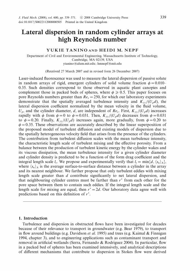
Figure 1. Definition of key geometric parameters for an array of cylinders of uniform diameterd . (a) In a random array, the centre-to-centre distance to the nearest neighbour, snc , differsfor each cylinder. (b) In a periodic square array, the centre-to-centre distance to the nearestneighbour is s + d ≡ 1/

√m for all cylinders, where m is the number of cylinders per unit area.

by Koch & Brady (1985). In packed beds of spheres, the solid volume fraction φ

is approximately constant at φ ≈ 0.6 (e.g. Mickley, Smith & Korchak 1965; Jolls &Hanratty 1966; Han, Bhakta & Carbonell 1985; Yevseyev, Nakoryakov & Romanov1991; Dullien 1979, p. 132). In contrast, previous studies on emergent (i.e. spanningthe water column and penetrating the free surface), rigid aquatic vegetation havefocused on low solid volume fraction arrays (φ = 0.0046–0.063, e.g. Nepf, Sullivan &Zavistoski 1997; White & Nepf 2003). Such sparse arrays are characteristic of saltmarshes, for example, where φ = 0.001–0.02 (Valiela, Teal & Deuser 1978; Leonard &Luther 1995). However, φ in aquatic plant canopies can approach that of packed beds.In mangroves, for example, φ can reach 0.45 because of the dense network of roots(Mazda et al. 1997). In constructed wetlands, φ may extend to 0.65 (Serra et al. 2004),and in this context Serra et al. (2004) reported lateral dispersion measurements at lowReynolds numbers in random arrays of φ = 0.10, 0.20 and 0.35. This paper investigatesturbulence and solute transport in arrays of randomly distributed, emergent, rigidcylinders of φ =0.010–0.35 in turbulent flow. Models for turbulence intensity and netlateral dispersion are presented and verified with laboratory measurements.

In § 2, we present a model for the mean turbulence intensity and the lateraldispersion coefficient as a function of cylinder distribution and cylinder density.In § 3, the experimental procedure for measuring turbulence, the integral length scaleand net lateral dispersion is described. In § 4, the experimental results are presentedand compared with the theory. Also, in Appendix A, analytical expressions of nearest-neighbour distances in a random array of cylinders of finite volume are presented,and parameters relevant to the models are derived.

2. Background theoryWe consider a homogeneous, two-dimensional array of rigid circular cylinders of

uniform diameter d distributed randomly with a constant density m (cylinders per unithorizontal area). The corresponding solid volume fraction is φ = mπd2/4. The centre-to-centre distance from a particular cylinder to its nearest neighbour is denotedby snc, as illustrated in figure 1(a) for an arbitrary cylinder. The corresponding

Lateral dispersion in random cylinder arrays 341

surface-to-surface distance is denoted by sn (= snc − d). Analytical expressions of〈sn〉A, the mean nearest-neighbour separation defined between cylinder surfaces, arederived in Appendix A. 〈〉A denotes an average over many cylinders in the array.The Cartesian coordinates x = (x, y, z) = (x1, x2, x3) are defined such that the x-axis isaligned with 〈u〉, the fluid velocity averaged over time and the fluid volume. The y-axisis in the horizontal plane and perpendicular to the x-axis (figure 1a). The verticalz-axis is aligned with the cylinder axes. Flow in a cylinder array is characterized bythe cylinder Reynolds number, Red ≡ 〈u〉d/ν, where ν is the kinematic viscosity, aswell as the Reynolds number based on a mean pore scale, Res ≡ 〈u〉s/ν. Here, themean pore scale s ≡ 1/

√m − d is defined as the surface-to-surface distance between

aligned cylinders in a square array with the same φ, as illustrated in figure 1(b).

2.1. Solute transport in a random array

Species conservation is described by the expression

∂c

∂t+ v · ∇c = −∇ · (−D0∇c), (2.1)

where t is time, c(x, t) is the solute concentration, v(x, t) = (u, v, w) = (v1, v2, v3) isthe fluid velocity and D0 is the molecular diffusion coefficient. In obstructed turbulentflows, it is convenient to first decompose c and v into a local time average andinstantaneous deviations from that average, and to farther decompose the time-averaged parameters into a spatial average and local deviations from that average(e.g. Raupach & Shaw 1982; Finnigan 1985). The temporal averaging operation,denoted by an overbar, is defined with a time interval much longer than the timescales of turbulent fluctuations and vortex shedding. The spatial averaging operation,denoted by 〈〉, is defined with an infinitesimally thin volume interval Vf that spansmany cylinders. The solid (cylinder) volume is excluded from Vf . Then, c = 〈c〉(x, t)+c′′(x, t) + c′(x, t) and v = 〈v〉(x, t) + v′′(x, t) + v′(x, t), where ′′ denotes the spatialfluctuations of the temporal average and ′ denotes the temporal fluctuations. Bydefinition, c′, v′, 〈c′′〉, 〈v′′〉 =0. Also, 〈v〉 = 〈w〉 =0. Substituting these expressions into(2.1), averaging over the same temporal and spatial intervals, and retaining only thedominant terms yield (Finnigan 1985, equation 21)

∂〈c〉∂t

+ 〈vj 〉∂〈c〉∂xj

= − ∂

∂xj

{⟨v′

j c′⟩

+ 〈v′′j c

′′〉 − D0

⟨∂

∂xj

(〈c〉 + c′′)

⟩}. (2.2)

In addition to fluxes associated with the local temporal fluctuations,⟨v′c′⟩, the

averaging scheme introduces dispersive fluxes associated with the time-averagedspatial fluctuations, 〈v′′c′′〉.

Laboratory measurements by White & Nepf (2003) and in the present study (seefigure 16) suggest that net dispersion is Fickian. Then, (2.2) simplifies to

∂〈c〉∂t

+ 〈vj 〉∂〈c〉∂xj

= Kjj

∂2〈c〉∂x2

j

, (2.3)

where Kjj are the coefficients for net dispersion. In this paper, we are concerned withKyy , the net lateral dispersion coefficient.

Farthermore, 〈v′c′〉 and 〈v′′c′′〉, like molecular diffusion, are expected to be Fickianif the spatial scale of the contributing mechanisms is smaller than the scale overwhich the mean concentration gradient varies (Corrsin 1974; Koch & Brady 1985;White & Nepf 2003). The two mechanisms associated with

⟨v′c′⟩

and 〈v′′c′′〉, asidentified below, both have characteristic scales of d and 〈sn〉A (§ 2.2 and § 2.3).


Because the dimensions of the averaging volume Vf are much larger than d and〈sn〉A by definition, 〈c〉 is expected to vary slowly at these spatial scales. Therefore,〈v′c′〉 and 〈v′′c′′〉 are expected to be Fickian. Consequently, Kyy is expected to be

the linear sum of three constant coefficients, one that parameterizes 〈v′c′〉, one thatparameterizes 〈v′′c′′〉 and the molecular diffusion coefficient. The first two coefficientsrepresent, respectively, (i) turbulent diffusion and (ii) mechanical dispersion (i.e.independent of molecular diffusion) due to the spatially heterogeneous velocity fieldgenerated by the randomly distributed cylinders. In this paper, the two processesare treated as independent, and one is not considered in the description of the other.Molecular diffusion is negligible, as we only consider turbulent flow.

2.2. Contribution from turbulence

The classic scaling for turbulent diffusion is Kyy ∼ 〈√

kt〉le, where le is the length scale

associated with mixing due to turbulent eddies and kt ≡ (u′2 + v′2 + w′2)/2 is theturbulent kinetic energy per unit mass (e.g. Baldyga & Bourne 1999, chapter 4).Previously, Nepf (1999) assumed that, in a cylinder array, le is equal to theintegral length scale of the largest turbulent eddies, lt , and that lt = d when cylinderspacing is smaller than the water depth. Then, Kyy ∼ 〈

√kt〉d . Nepf (1999) fitted this

turbulent diffusion scale to experimental observation at Res =Ups/ν = 2000–10 000in a φ =0.0046, periodic, staggered cylinder array (see Zavistoski 1994 for the exactcylinder configuration) to obtain

Kyy

Upd= 0.9

⟨√kt

Up

⟩. (2.4)

The mean pore velocity Up is the average of u over all fluid volume within the array,

and is determined as Up = Q/[〈H 〉W (1 − φ)], where Q is the volumetric flow rate,

〈H 〉 is the mean water depth and W is the width of the laboratory flume in which thearray was contained. Note that 〈u〉 ≈ Up if the thickness of the boundary layers at

the bed and sidewalls of the flume is negligible relative to 〈H 〉 and W . Equation (2.4)is inconsistent with experiment at high φ, as will be demonstrated in § 4.3. Below,we propose a new scale model for turbulent diffusion, in which le and lt may beconstrained by cylinder spacing at high φ.

2.2.1. Turbulence intensity

The functionality of the mean turbulence intensity, 〈√

kt/〈u〉〉, can be predictedfrom the temporally and spatially averaged mean and turbulent kinetic energybudgets in the array (see e.g. Raupach, Antonia & Rajagopalan 1991, equation 4.3a, b

or Kaimal & Finnigan 1994, equation 3.40 for the turbulent kinetic energy budget).

In cylinder arrays, a wake production term, −⟨u′

iu′j

′′∂ui

′′/∂xj

⟩(� 0), accounts for

turbulence production by the cylinder wakes. Numerical simulation by Burke &Stolzenbach (1983, figure 5.23) demonstrates for CD〈H 〉φ/(πd/4) = 0.01–1.0, whereCD is the coefficient of mean cylinder drag, that wake production exceeds productiondue to shear within the cylinder array, except near the bed. In fully developed flowwith negligible shear production, the turbulent kinetic energy budget reduces to abalance between wake production and viscous dissipation of turbulent kinetic energy(e.g. Burke & Stolzenbach 1983; Raupach & Shaw 1982):

0 ≈ −⟨

u′iu

′j

′′ ∂ui′′

∂xj

⟩− ν

⟨∂ui

∂xj

′ ∂ui

∂xj

′⟩

. (2.5)


Similarly, the mean kinetic energy budget reduces to

0 ≈ 〈ui〉f formi +

⟨u′

iu′j

′′ ∂ui′′

∂xj

⟩+ ν⟨ui

′′∇2ui′′⟩, (2.6)

where

fformi =

1

ρVf

∫∫Sc

pni dS (� 0) (2.7)

is the hydrodynamic force per unit fluid mass exerted on Sc that arises from thepressure loss in cylinder wakes, where Sc denotes all cylinder surfaces that intersectVf , n is the unit normal vector on Sc pointing out of Vf , p(x, t) is the local pressureand ρ is the fluid density.

The Kolmogorov microscale η estimated from our laser Doppler velocimetry (LDV)measurements (see § 3) ranged from η/d = 0.0014 to η/d = 0.21 and η/〈sn〉A = 0.0036to η〈sn〉A =0.83. These O(0.001–1) ratios suggest that wake production is a moresignificant sink of mean kinetic energy than the viscous term ν〈ui

′′∇2ui′′〉 (Raupach &

Shaw 1982). For simplicity, the latter is neglected in (2.6), which yields a balancebetween the rate of work done by form drag and wake production (Raupach & Shaw1982, equation 17):

0 ≈ 〈ui〉f formi +

⟨u′

iu′j

′′ ∂ui′′

∂xj

⟩. (2.8)

Note that i = 1 is the only non-zero component of 〈ui〉f formi . Combining (2.5) and

(2.8) and replacing the viscous dissipation term with the classic scaling,√

kt3/lt

(Tennekes & Lumley 1972), yield a model for mean turbulence intensity:⟨√kt

〈u〉

⟩∼[

〈fD〉form

ρ〈u〉2d/2

lt

d

md2

2(1 − φ)

]1/3, (2.9)

where 〈fD〉form ≡ ρ(1 − φ)f form1 /m is the inertial contribution to the mean drag (in the

direction of mean flow) per unit length of cylinder. Tanino & Nepf (2008, d =0.64 cm)determined the following empirical relation for 〈fD〉form

H , the depth average of 〈fD〉form:

〈fD〉formH

ρU 2pd/2

= 2 [(0.46 ± 0.11) + (3.8 ± 0.5)φ] . (2.10)

For convenience, we define a drag coefficient that represents this contribution:

CformD ≡

⟨fD

⟩form

H

ρU 2pd/2

. (2.11)

Laboratory measurements suggest that temporally and spatially averaged flowproperties in Tanino & Nepf (2008)’s laboratory experiments and in the presentstudy were approximately uniform vertically (e.g. figure 8; White & Nepf 2003) andlaterally (e.g. figure 7; White & Nepf 2003). Consequently, 〈fD〉form ≈ 〈fD〉form

H and〈u〉 ≈ Up . Then, (2.9) can be rewritten as:⟨√

kt

〈u〉

⟩≈⟨√

kt

Up

⟩∼[C

formD

lt

d

φ

(1 − φ)π/2

]1/3, (2.12)

where CformD is described by (2.10) and (2.11). Recall that m =φ/(πd2/4).

The choice of lt = d is the convention in the literature on flow through vegetation(e.g. Raupach & Shaw 1982; Raupach et al. 1991) and is reasonable in sparse arrays


10 20

10

20

(b)

10 20

10

20

x/d x/d

yd

(a)

Figure 2. A section of simulated arrays of (a) φ = 0.010, d < 〈sn〉A and (b) φ = 0.20, d > 〈sn〉A.Circles represent cylinders, to scale. Turbulent eddies, depicted by the arrows, are O(d) insparse arrays, but are constrained by the local cylinder separation where the pore length scaleis smaller than d .

(figure 2a). In dense arrays, however, the local pore length scale may be less thanO(d). In these regions, physical reasoning suggests that the local cylinder spacingwill constrain the eddies (figure 2b). Therefore, lt must be redefined at high φ. Thesimplest function consistent with the expected dependence on the local surface-to-surface distance between cylinders is

lt = min{d, 〈sn〉A}. (2.13)

2.2.2. Turbulent diffusion coefficient

We expect the spatially heterogeneous velocity field to induce lateral deflections ofO(d) per cylinder in the dispersion mechanism described in § 2.3 (e.g. Masuoka &Takatsu 1996; Nepf 1999). Therefore, we propose that only turbulent eddies withmixing length scale le � d contribute significantly to net lateral dispersion relative tothe spatially heterogeneous velocity field. Let r∗ be the minimum distance betweencylinder centres that permits the pore space constrained by them to contain sucheddies. Physical reasoning suggests that the mixing length scale associated withturbulent eddies is approximately equal to the size of the eddies, i.e. le ≈ lt , which,together with (2.13), implies r∗ − d = d . Then, within an infinitesimally thin sectionof the array whose total (solid and fluid) volume is denoted by V , the sum of allvolume that contributes to turbulent diffusion, Vm (� V ), is a sum of all pore spacewith length greater than r∗ − d . Within these pores, le = d . To simplify, we associateall fluid volume with a cylinder. Farther, each cylinder in the array has a fluid volumearound it of characteristic horizontal area s2

n . Then,

Vm =⟨s2n

⟩snc>r∗Nsnc>r∗, (2.14)

where Nsnc > r∗ is the number of cylinders with snc > r∗ in V . Recall that snc = sn + d .To define Kyy as an average over both fluid and solid volume, local

√kt le is

integrated over Vm and divided by V . Then, the contribution from turbulent diffusion


is

Kyy

〈u〉d = γ1

〈√

kt le〉m

〈u〉dVm

V, (2.15)

where 〈〉m denotes a spatial average over Vm and γ1 is the scaling constant.Equation (2.15) is simplified by neglecting the cross-correlations such that〈√

kt le〉m = 〈√

kt〉m〈le〉m and assuming that 〈√

kt〉m = 〈√

kt〉, the average over all fluidvolume. Equation (2.15) then becomes

Kyy

〈u〉d ≈ γ1

⟨√kt

〈u〉

⟩〈s2

n〉snc>r∗

d2

φ

π/4Psnc>r∗, (2.16)

where Psnc > r∗ ≡ Nsnc > r∗/(mV ) is the fraction of cylinders with a nearest neighbourfarther than r∗ (centre-to-centre) from its centre. Recall that 〈

√kt/〈u〉〉 can be

described by (2.12) and (2.13), given d and φ.

2.3. Contribution from the time-averaged, spatially heterogeneous velocity field

Two existing models of lateral dispersion due to the spatially heterogeneous velocityfield are considered in this paper. The simplest model describes the lateral deflection offluid particles due to the presence of the cylinders as a one-dimensional random walk(Nepf 1999). In this model, a fluid particle is considered to undergo a sequenceof independent and discrete lateral displacements of equal length, where eachdisplacement has equal probability of being in the positive or in the negative y

direction. The long-time lateral dispersion of many such fluid particles is describedby:

Kyy

〈u〉d =1

2

( ε

d

)2 φ

π/4, (2.17)

where ε, the magnitude of each displacement, is a property of the cylinderconfiguration and Red . Nepf (1999) proposed that ε = d . With this assumption, (2.17)becomes a function of φ only.

The second model considered for this mechanism is Koch & Brady (1986)’sanalytical solution for mechanical dispersion due to two-cylinder interactions inStokes flow, with a modification to only include cylinders with a nearest neighboursufficiently close to permit cylinder–cylinder interaction. Analytical solutions for long-time Fickian dispersion in a homogeneous, sparse, random cylinder array were derivedfor Stokes flow by Koch & Brady (1986) by averaging the governing equations overan ensemble of arrays with different cylinder configurations. Neglecting moleculardiffusion, lateral dispersion arises from the velocity disturbances induced by therandomly distributed cylinders (Koch & Brady 1986). The authors demonstratethat this hydrodynamic dispersion consists of a mechanical component and non-mechanical corrections, but that only the mechanical contribution, associated withthe spatially heterogeneous velocity field due to the obstacles, has a non-zerolateral component. Farther, the authors showed that, because of their fore–aftsymmetry, circular cylinders do not contribute to lateral dispersion unless two-cylinder interactions are considered. Taking into consideration such interactions,Koch & Brady (1986) determined that the mechanical contribution of the cylinderarray in Stokes flow is

Kyy

〈u〉d =π

4096

(d2

k⊥

)3/21 − φ

φ2, (2.18)


where k⊥ is the permeability such that the mean drag (in the direction of mean flow)per unit length of cylinder is ⟨

fD

⟩=

π

4

d2

k⊥μ〈u〉1 − φ

φ, (2.19)

where μ is the dynamic viscosity. Numerical simulations show that d2k−1⊥ increases

monotonically with φ (Koch & Ladd 1997). For sparse random arrays, k⊥ is accuratelydescribed by Spielman & Goren (1968)’s analytical solution (B 1). For dense arrays,Koch & Ladd (1997) have shown that a theoretical model based on the lubricationapproximation accurately captures the dependence of k⊥ on the characteristic distancebetween neighbouring cylinders. The permeability k⊥ for arrays of intermediatedensity, for which analytical expressions have not been derived, can be describedby an empirical fit to numerical simulation data (B 3). Models for k⊥ relevant to ourlaboratory experiments are discussed in Appendix B.

Equation (2.18), where k⊥ is described by (B 1), predicts that dispersion due totwo-cylinder interactions will increase as φ decreases below φ = 0.017. Koch & Brady(1986) attribute this predicted increase to the increase in the average distance overwhich velocity disturbances induced by a cylinder decay. This distance, known as theBrinkman screening length, scales with the square root of permeability. As discussedin Appendix B,

√k⊥ ≈ 〈sn〉A in sparse arrays. However, the fraction of cylinders with

a neighbour close enough to result in cylinder–cylinder interaction decreases withdecreasing φ, and physical reasoning suggests that the contribution from this processapproaches zero as φ decreases to zero. Therefore, we introduce an adjustment to Koch& Brady (1986)’s solution. Previous studies in unsteady and turbulent flow reportinteracting wakes between side-by-side cylinders with a centre-to-centre distance lessthan 5d (e.g. Zhang & Zhou 2001; Meneghini et al. 2001). Similarly, the drag ona cylinder is influenced by the presence of a neighbouring cylinder that is within5d (Petryk 1969). Following these studies, we assume that only cylinders whosecentres are within 5d of another cylinder centre contribute to net dispersion throughthis mechanism. Accordingly, Koch & Brady (1986)’s solution is multiplied by thefraction of cylinders that have a nearest neighbour within 5d , Psnc<5d . We assumethat this process is otherwise unaffected by inertia. In addition, a scaling constantγ2 is introduced. After the introduction of these two terms, Koch & Brady (1986)’ssolution becomes

Kyy

〈u〉d = γ2Psnc<5d

π

4096

(d2

k⊥

)3/21 − φ

φ2. (2.20)

2.4. Coefficient for net lateral dispersion

Finally, an expression for net lateral dispersion is given by the linear superposition ofthe models for turbulent diffusion and dispersion due to the spatially heterogeneousvelocity field. For example, superposing (2.16) and the proposed modification ofKoch & Brady (1986)’s solution (2.20) yields

Kyy

〈u〉d = γ1

4

πφ

⟨√kt

〈u〉

⟩Psnc>r∗

⟨s2n

⟩snc>r∗

d2+ γ2Psnc<5d

π

4096

(d2

k⊥

)3/21 − φ

φ2. (2.21)

To permit an analytical expression for (2.21), Psnc > r∗ and Psnc < 5d are approximatedas the probability that a single cylinder in a random array will have a nearestneighbour farther away than r = r∗ and within r = 5d , respectively, where r is the radialcoordinate defined with the origin at the centre of that cylinder. Analytical expressions


Figure 3. A photo of a section of the model φ = 0.27 array in plan view.

for Psnc > r∗ , Psnc < 5d and 〈s2n〉snc > r∗ for the random arrays used in the present laboratory

experiments are derived in Appendix A. Note that Psnc < 5d approaches 1 monotonicallyas φ increases from zero, with Psnc < 5d > 0.99 at φ � 0.043. Expressions for k⊥ arepresented in Appendix B.

3. Experimental procedureLaboratory experiments were conducted to verify the definition of lt (2.13) and the

scale model for 〈√

kt/〈u〉〉 (2.12) and to document the φ dependence of Kyy/(〈u〉d).Scaling constants in (2.12) and the model for Kyy/(〈u〉d) (2.21) were determined fromthe experimental data.

The laboratory study consisted of two parts: measuring velocity and imaging thelateral concentration profile of a passive tracer. In both parts, cylindrical mapledowels of diameter d = 0.64 cm (Saunders Brothers, Inc.) were used to create arraysof eight densities: φ = 0.010, 0.020, 0.031, 0.060, 0.091, 0.15, 0.20 and 0.35 for thevelocity measurements and φ = 0.010, 0.031, 0.060, 0.091, 0.15, 0.20, 0.27 and 0.35for the tracer study. All arrays, except for the φ =0.031 arrays, were created incustom-made 71.1 cm × 40.0 cm perforated polyvinyl chloride (PVC) sheets of either20% or 35% hole fraction. The locations of the holes in these sheets were definedby generating uniformly distributed random coordinates for the hole centres until thedesired number of non-overlapping holes was assigned; these non-overlapping holeswere drilled into the sheets. Here, “non-overlapping” holes were defined to have noother hole centre fall within a 2d × 2d square around their centres. Any directionalbias resulting from this definition, instead of defining the overlap over a circle ofradius d , is assumed negligible. The φ = 0.20 and 0.35 arrays were created by fillingall of the holes. The φ =0.010, 0.020, 0.060, 0.091, 0.15 and 0.27 arrays were createdby selecting the holes to be filled or to be left empty using MATLAB’s randomnumber generator. The φ = 0.031 array in the tracer study was created by partiallyfilling 20% hole fraction PVC sheets with 1/2-inch staggered hole centres (AmetcoManufacturing Corporation). The φ = 0.031 array used in the velocity measurementswere created by partially filling Plexiglas boards that were designed by White & Nepf(2003). Note that White & Nepf (2003) defined non-overlapping holes to have noother hole centre fall within a concentric circle of diameter 4d . In the tracer study,the dowels were inserted into four PVC sheets placed along the bed of the workingsection of the flume. A plan view of a section of the φ = 0.27 array is presented infigure 3. For the velocity measurements, different numbers of PVC sheets were used


φ array base d/〈sn〉A array length [cm] xgap [cm] n

0.010 PVC 0.28 569.0 0.0 1180.020 PVC 0.43 497.8 0.0 1470.031 Plexiglas 0.49 498.8 0.0 2610.060 PVC 0.93 284.5 0.0 2600.091 PVC 1.3 284.5 0.7 – 1.3 1910.15 PVC 2.0 213.4 0.0 1950.20 PVC 2.7 213.4 0.0, 0.1 1360.35 PVC 5.9 106.1 0.3, 0.6 116, 22

Table 1. Array setup for LDV measurements. xgap is the width of the gap that wascreated in the cylinder array to permit multiple LDV measurements in each lateral transect.xgap = 0.0 indicates an unmodified array. n is the total number of time records collected atRes ≡ Ups/ν > 250 (φ = 0.010–0.20) and both Res > 200 and Res > 250 for φ = 0.35.

(see table 1) because the density of cylinders increases with φ and a shorter arraylength is required to achieve fully developed conditions at higher φ. The cylinders areperpendicular to the horizontal bed of the working section of the flume.

As stated previously, velocity measurements taken in emergent cylinder arrays byWhite & Nepf (2003) and in the present study (e.g. figures 7 and 8) have shownthat 〈u〉 is approximately constant within the array, except very close to the bedand the sidewalls. Therefore, 〈u〉 is approximated by Up , measured as the time-

averaged volumetric flow rate divided by the width of the working section, 〈H 〉 atthe measurement location, and 1 − φ. Similarly, Reynolds numbers were calculatedusing Up as the velocity scale.

3.1. Velocity measurements

Velocity measurements were taken in a 670 cm × 20.3 cm × 30.5 cm recirculatingPlexiglas laboratory flume using two-dimensional LDV (Dantec MeasurementTechnology). The time-averaged water depth at the LDV sampling volume rangedfrom 〈H 〉 =13.1 cm to 〈H 〉 =22.1 cm. Flow was generated by a centrifugal pump andmeasured with an in-line flow meter. At each φ, time records of longitudinal andvertical velocity components were collected at positions (s +d)/4 apart along a lateraltransect at several streamwise positions within the array for a range of Res . Thelateral transects were at an elevation of 2〈H 〉/3 from the bed.

In total, 2107 time records were collected. The time average (u, w), the temporaldeviations (u′, w′) and the variance (u′2, w′2) were calculated for each record as

u =

∑k

uktk∑k

tk, (3.1)

u′k = uk − u (3.2)

and

u′2 =

∑k

u′2k tk∑

k

tk, (3.3)


respectively, where tk is the residence time of the kth seeding particle in the LDVsampling volume. The vertical components are defined analogously. Note that onlyu(t) and w(t) could be measured. However, previous measurements indicate v′2 ≈ u′2

(Tanino & Nepf 2007), and the turbulent kinetic energy per unit mass, kt , wasdetermined as kt = (2u′2 + w′2)/2.

The integral length scale lt can be estimated from the time record of turbulentfluctuations. Specifically, |u|/(2πfpeak,vj

), where fpeak,vjis the frequency at which the

frequency-weighted power spectral density of v′j peaks, is approximately equal to the

Eulerian integral length scale (Kaimal & Finnigan 1994, p. 38) and is one measure oflt (e.g. Pearson, Krogstad & van de Water 2002). To determine fpeak,vj

, u′(t) and w′(t)records were resampled at uniform time intervals by linear interpolation. The shortestinterval between consecutive samples in that time record was used as the interval.The power spectral densities [cm2 s−2 Hz−1] of the reevaluated u′(t) and w′(t) weredetermined using MATLAB’s pwelch.m function. A peak at 120 Hz exists in mostrecords, which is attributed to background noise. Because this frequency is one orderof magnitude higher than the maximum Up/d and Up/s in our experiments, whichwere 15 Hz and 30 Hz, respectively, it is assumed that this noise did not interferewith the analysis. Also, the resampled record is accurate only to f = fraw/(2π),where fraw is the mean data rate of the raw time record (Tummers & Passchier2001). Accordingly, frequencies above fraw and 110 Hz were neglected in the analysis.Finally, lt was estimated from the frequency fpeak,u corresponding to the peak in thefrequency-weighted power spectral density of the resampled u′(t) as

lpeak,u ≡ |u|2πfpeak,u

. (3.4)

The vertical length scale, lpeak,w , was determined from the power spectral density of w′

analogously. Of a total of 1317 lpeak,u measurements at Res � 250, ten were discardedbecause they differed from the mean lpeak,u for that φ by more than three standarddeviations and three were discarded because a peak could not be identified in thefrequency-weighted spectrum.

Alternatively, lt can be estimated from the autocorrelation function of the localvelocity fluctuation as

lcorr,u ≡ |u|∫ τ0

0

u′(t)u′(t + τ )

u′2dτ, (3.5)

where τ is the time lag with respect to t and τ0 is τ at the first zero-crossing.MATLAB’s xcov.m function was used to calculate the variance-normalized auto-correlation function of each resampled u′(t) record, from which the Eulerian integrallength scale lcorr,u (3.5) was calculated. Of a total of 1290 time records at Res � 250for which lcorr,u could be computed, 22 were discarded because the calculated lcorr,u

deviated from the mean for that φ by more than three standard deviations.The spatial heterogeneity of the velocity field is quantified by the variance of

u′′ = u(t) − Up (e.g. White & Nepf 2003),

σ 2u′′

U 2p

=

⟨u′′2

U 2p

⟩−⟨

u′′

Up

⟩2

. (3.6)

Specifically, measurements of u for each φ were separated into five or six groupsbased on Up . For each (φ, Up) group, σ 2

u′′/U 2p and the maximum and minimum Red

were computed.


0 2 4 6 8

0

1

2

(a) (b)

(c) (d)

(e) ( f )

0 2 4 6 8

0

1

2

0 2 4 6 8

0.4

0.8

0 2 4 6 8

0.4

0.8

0 2 4 6 8

0.5

1.0

1.5

Δxgap/�sn�A Δxgap/�sn�A

0 2 4 6 8

0.5

1.0

1.5

Figure 4. Sensitivity of (a) 〈u/Up〉, (b) 〈w/Up〉, (c) 〈u′2/U 2p〉, (d ) 〈w′2/U 2

p〉, (e) 〈lpeak,u〉/d and

(f ) 〈lpeak,w〉/d , as defined by (3.1)–(3.4), to xgap , the width of the gap in the array at thesampling locations. Ten or eleven time records were collected at lateral intervals of (s + d)/2along a single lateral transect in a φ = 0.20 array for each xgap . Dots represent the local valuesand open markers represent the lateral average over each transect. Res = 430–480 (circle) andRes = 470–540 (square). Vertical bars indicate the standard error of the mean.

Except in the sparsest arrays, measurements could not be collected across theentire width of the flume because cylinders obstructed the LDV laser beams. Topermit sufficient sampling positions along each transect, gaps of normalized widthxgap/〈sn〉A =1.4–2.7, 0.0–0.4 and 3–6 were created in arrays of φ = 0.091, 0.20 and0.35, respectively (table 1). To determine whether these gaps biased the results, velocitytime records were collected along a lateral transect in a φ = 0.20 array for a rangeof xgap , from which lateral averages of u/Up , w/Up , u′2/U 2

p , w′2/U 2p , lpeak,u/d and

lpeak,w/d were calculated for each transect. The lateral averages, with the exception

of 〈w/Up〉 and 〈w′2/U 2p〉, remained within standard error of their respective values at

xgap/〈sn〉A =0.2 in the range xgap/〈sn〉A = 0.2 to 8.1 ± 0.4 (figure 4). The constantvalues suggest that our results were not biased by the gaps.


The duration of measurement at a single position was determined from the timetaken for the time average and the variance, as defined by (3.1)–(3.3), of preliminaryvelocity time records to converge to within 5% of their 20-minute average. This testwas performed for each φ for several Red . The duration varied from 60 s to 1000 s,with lower Red generally requiring a longer time to converge.

3.2. Tracer experiments

Laser-induced fluorescence (LIF) was used to measure the lateral dispersion coefficientin a recirculating Plexiglas laboratory flume with a 284 cm × 40 cm × 43 cm workingsection. LIF measurements could not be collected in the same flume as the LDVmeasurements because the seeding material used in the latter would have interferedwith the former. The use of the two flumes is justified because the spatially averagedturbulence characteristics are determined by the macroscopic array properties andare not specific to the flume system, as demonstrated by the good agreement in meanturbulence intensity and lpeak,u/d observed by White (2002) and in the present study(figures 12 and 15).

Dilute rhodamine WT was injected continuously from a horizontal needle witha syringe pump (Orion SageT M M362) at a rate that was matched visually withthe local flow. A single horizontal beam of argon ion laser (Coherent INNOVAR

70 ion laser) passed laterally through the flume at a single streamwise position x

downstream of the tracer source. A Sony CCD Firewire digital camera XCD-X710controlled by Unibrain Fire-i 3.0 application captured the line of fluoresced tracerfrom above the flume in a sequence of 1024 × 48 bitmap images. To filter out thelaser beam, 530 nm and 515 nm long-pass filters (Midwest Optical Systems, Inc.) wereattached to the camera. The fluorescence intensity is proportional to the rhodamineWT concentration. The correct spatial scale on the images was determined from aphoto of a ruler submerged horizontally in the position of the laser beam. The imageof the ruler was taken every time the local water depth, the camera setting or theposition of the laser beam or the camera changed. At high φ, cylinders were removedto create the 1.3-cm gap in the array necessary to insert this ruler. This gap alsoensured that the laser beam could pass through the entire width of the flume. Theposition of the laser beam relative to the tracer source, which was restricted by thedistance at which the tracer reached the sidewalls, ranged from x = 5 cm to x = 143 cm.The time-averaged water depth at the longitudinal position of the laser beam rangedfrom 〈H 〉 =9.1 cm to 〈H 〉 = 18.6 cm. Additional details of the experimental procedureare provided in Tanino & Nepf (2007).

Instantaneous intensity profiles were extracted from the bitmap images, correctedfor background and anomalous pixel intensities and averaged over the duration ofthe experiment to yield a time-averaged intensity profile, I (y, t). The time-averagedprofile was corrected for noise and background. Then, its variance was calculated as

σ 2(x) =M2(x)

M0(x)−[M1(x)

M0(x)

]2, (3.7)

where Mj (x) is the j th moment,

Mj (x) =

∫ κ1

κ2

yjI (y, t) dy. (3.8)

The zeroth, first and second moments and the corresponding σ were calculated bysetting the limits of integration in (3.8), κ1,2, at the two edges of the images. Next, κ1,2

were redefined as κ1,2 = (M1/M0) ± 3σ and the calculation was repeated. These limits


were applied to prevent small fluctuations at large distances from the centre of massfrom altering the variance estimate dramatically.

Previous evaluation of the experimental data determined that, within the range of x

considered in the present experiments, σ 2 at constant x increases with pore Reynoldsnumber until Res ≈ 250 and is constant at higher Res (Tanino & Nepf 2007, figure 4).In this study, we focus on Res > 250. The net lateral dispersion coefficient normalizedby Up and d for each φ was calculated as

Kyy

Upd=

1

2d

dσ 2

dx, (3.9)

where dσ 2/dx is the gradient of the line of regression applied to all σ 2 measurementsat Res > 200 for φ = 0.35 and at Res > 250 for all other φ. The criterion for φ = 0.35 islower because the experimental setup could not accommodate the large longitudinalfree surface gradient that results from the cylinder drag (Tanino & Nepf 2008) atRes > 250.

〈√

kt/Up〉 and Kyy/(Upd) at each φ were calculated as the gradient of the lineof regression of

√kt on Up and of σ 2 on x normalized by 2d , respectively. The

uncertainty in the gradient of each line of regression was estimated according toTaylor (1997, chapter 8). Consider the line y = B0 + B1x that best fits n data points(xk, yk), k = 1, 2, . . . , n in the least-squares sense. The uncertainty in B1 is defined as(Taylor 1997, equations 8.12, 8.15, 8.17)√√√√ 1

n − 2

n∑k=1

[yk − (B0 + B1xk)]2

√√√√√√n

n

n∑k=1

x2k −(

n∑k=1

xk

)2. (3.10)

The uncertainties in 〈√

kt/Up〉 and dσ 2/dx are calculated as (3.10). The uncertaintyin Kyy/(Upd) is simply the uncertainty in dσ 2/dx divided by 2d .

4. Experimental results4.1. Flow visualization

We first consider the qualitative Reynolds number dependence. Figures 5 and 6 presentunprocessed still photos taken in the φ =0.010 and 0.15 arrays, respectively, at fourdifferent Red . Recall from § 2 that Red is the Reynolds number based on d insteadof s, i.e. Red = Resd/s. In figure 5, fluorescein solution was injected approximately3.7 cm upstream of cylinder A. The injection point is visible at the top of the imagesin figure 6. The tracer emerges from the needle as a single distinct filament for allRed . In figure 6(a), the tracer is deflected by the cylinders and is advected throughthe array forming a streakline that is stationary in time. The flow is unsteady for allother conditions presented in figures 5 and 6 and, consequently, the angle at whichthe tracer encounters cylinders A and B in figure 5 and cylinder A in figure 6 varieswith time. In both arrays, the Red dependence is qualitatively the same. The tracerforms distinct, thin ( d) bands of dyed and undyed fluid at Red ≈ 30 (figures 5a and6a). At higher Red , turbulent eddies rapidly mix the fluid within the pores, resultingin a more spatially uniform distribution. For example, distinct filaments cannot bedistinguished at the bottom of the image in figures 5(d ) and 6(d ).

The φ =0.010 array is sufficiently sparse that individual vortex streets and theirinteractions can be identified. A laminar vortex street is seen behind cylinder B at


A

B

(a) (b)

(c) (d)

Figure 5. Flow visualization by fluorescein and blue lighting in a φ = 0.010 array at thefollowing values of Red : (a) 28 ± 1, (b) 56 ± 3, (c) 78 ± 3 and (d ) 113 ± 5. These valuescorrespond to Res = 220 ± 10, 430 ± 20, 600 ± 20 and 880 ± 40, respectively. Mean flow isfrom top to bottom. Camera and dye injection position were fixed. The injection point isapproximately 3.7 cm upstream of cylinder A.

(a) (b)

(c) (d)

A

Figure 6. Flow visualization by fluorescein and blue lighting in a φ = 0.15 array at thefollowing values of Red : (a) 32 ± 2, (b) 73 ± 3, (c) 108 ± 4 and (d ) 186 ± 7. These valuescorrespond to Res = 42 ± 2, 94 ± 4, 139 ± 6 and 240 ± 9, respectively. Mean flow is from topto bottom. Camera and dye injection position were fixed.


0 10 20 30

0

1

2(a)

0 10 20 30

0

1

2

y/d

(b)

Figure 7. Lateral transects of u/Up (solid line) and√

kt/Up (grey, dashed line) at (a) φ =0.010, Res = 620–690 (dot), 1600–1700 (×), 2400–2600 (�), 2700–2900 (square), and3100–3300 (+) and at (b) φ = 0.15, Res = 130–140 (dot), 400–430 (+), and 510–600 (∗). Flumesidewalls were at y = 0 and 32.0d .

Red =28±1 (figure 5a). In contrast, a pair of standing eddies are attached to cylinderA in the same image. Here, tracer emerges O(d ) downstream of the cylinder as asingle, straight filament. The difference between the wakes of cylinders A and B canbe attributed to differences in the local flow conditions due to the random natureof the cylinder distribution. At an isolated cylinder, standing eddies form at Red ≈ 5and become unsteady at Red ≈ 40 (Lienhard 1966). In figure 5(a), Red = 28 ± 1, andan isolated wake is expected to be steady. The presence of neighbouring cylindersmay have elevated the local Red such that flow around cylinder B enters the unsteadyregime. Figure 5(a) also highlights the interaction of the wakes. The single tracerfilament leaving cylinder A is drawn into the vortex street of cylinder B as itpropagates downstream. At Red = 78 ± 3, cylinders A and B both shed vortices(figure 5c). Moreover, the shedding is in phase, indicating wake interaction. Here,the centre-to-centre distance between cylinders A and B is approximately 4d , and theoccurrence of wake interaction is consistent with (2.20). The vortex street from thetwo cylinders appears to merge and form a single turbulent street at approximatelyx ≈ 15d . This is consistent with Williamson (1985)’s observations of in-phase vortexshedding behind a pair of side-by-side cylinders. A similar merging of vortex streetscan be identified downstream of four cylinders in a square configuration at a 45◦

angle to the flow (Lam, Li, Chan & So 2003, figure 9, Red = 200).

4.2. Velocity and turbulence structure

Local velocity varies dramatically in the horizontal plane due to the randomconfiguration of the cylinders. This is highlighted in figure 7, in which each subplotpresents lateral transects of time-averaged and turbulent components of velocity ata single longitudinal position. For example, the time average of the longitudinalcomponent of velocity (u) deviates dramatically from its cross-sectional average (Up)at all φ and Res . Indeed, u is negative at certain positions in the array because ofrecirculation zones that develop immediately downstream of a cylinder (figure 7b).


0 1 20

0.2

0.4

0.6

0.8

1.0

u/Up, �u/Up�

(a) (b)

z�H�

0 0.25 0.5 0.750

0.2

0.4

0.6

0.8

1.0

√kt/Up, �√kt/Up�

Figure 8. Vertical profiles of (a) u/Up and (b)√

kt/Up at four positions, 1.0d apart, along alateral transect (×). The lateral average of the four profiles is presented as a thick solid line.Horizontal bars reflect the uncertainty in Up . φ = 0.20, Res = 440–490, 〈H 〉 = 17.3–17.4 cm.

A comparison of lateral profiles at different Res at the same position in the arrayindicates that the shape of the lateral profiles remains constant as Res varies (figure 7),confirming that the spatial variability is largely dictated by the cylinder configuration.Because the array is vertically uniform, vertical variations in the time-averaged velocityand turbulence intensity are expected to be smaller than their lateral heterogeneity.In particular, spatial averages 〈u/Up〉 and 〈

√kt/Up〉 are approximately uniform in

depth (solid lines in figure 8). Similar observations were made in random arrays ofφ = 0.010, 0.020 and 0.063 by White & Nepf (2003). Finally, note that the spatialvariability is smaller in figure 7(a) (φ = 0.010) than in figure 7(b) (φ =0.15). Indeed,σ 2

u′′/U 2p increases with φ, as illustrated in figure 9 for mean Red = 340–440.

Like u and√

kt , the power spectrum and the autocorrelation function varydramatically in the horizontal plane. The frequency-weighted power spectral densityand the autocorrelation function of selected u′(t) records are presented in figure 10for reference.

The two methods for estimating the integral length scale yield similar values, asexpected (figure 11). Therefore, only 〈lpeak,u/d〉 is compared with lt here (figure 12).The measured integral length scale generally decreases with increasing d/〈sn〉A, asdemonstrated by 〈lpeak,u/d〉, where the spatial average was calculated as the meanof all LDV measurements at Res � 250 at each φ. Equation (2.13) captures thisdecrease of 〈lpeak,u/d〉 reasonably well for d/〈sn〉A � 1.3. As expected from (2.13),the mean of 〈lpeak,u/d〉 for d/〈sn〉A < 0.5 is 1.0. However, 〈lpeak,u/d〉 decreases withincreasing d/〈sn〉A below d/〈sn〉A = 1 in both the present study and in White (2002)’sexperiments. Additional measurements are necessary to verify (2.13) for d/〈sn〉A < 1.

The mean turbulence intensity at a given φ, 〈√

kt/Up〉, is calculated as the gradientof the line of regression of all LDV measurements of

√kt on Up for Res > 250

at φ < 0.35 and for Res > 200 at φ =0.35. The Res ranges match those for which


0.1 0.2

φ

0.30

0.2

0.4

σu′′Up

2

2

Figure 9. Normalized spatial variance of u′′, σ 2u′′/U 2

p , for mean Red = 340–440: (φ, Red ) =(0.010, 410), (0.020, 360), (0.020, 410), (0.031, 390), (0.060, 390), (0.15, 340), (0.20, 430), and(0.35, 430). Two sets of σ 2

u′′/U 2p were calculated from (3.6): one using the upper estimates of

Up and the other using the lower estimates. The ends of the vertical bars reflect these twoestimates; the marker is their mean.

0 0.5 1.0 1.5

0.2

0.4

(a)

0 0.5 1.0

0

0.5

1.0

0 2 4

1

2

(b)

0 10 200

0.5

1.0

2 4 60

15

30

(c)

fd/|u|

0 0.1 0.2 0.30

0.5

1.0

τ (s)

Figure 10. The frequency-weighted power spectral density (cm2 s−2) (left) and the variance-normalized autocorrelation function (right) of selected u′ time records: (a) φ = 0.010, u =3.8 cm s−1, Res =2700, (b) φ =0.20, u = −1.4 cm s−1, Res =320 and (c) φ = 0.35, u= 4.9 cm s−1,Res = 380. Arrows mark the identified peak in the frequency-weighted power spectraldensity (left) and τ0 (right). f denotes frequency.


10–3 10–2 10–1 100 101

101

100

10–1

10–2

10–3

lcorr, u

lpeak,u/d

d

1:1

Figure 11. Comparison of lpeak,u (3.4) and lcorr,u (3.5) determined from LDV measurementsat Res � 250 and φ = 0.010 (∗), 0.020 (star), 0.031 (·), 0.060 (♦), 0.091 (+), 0.15 (square),0.20 (×), and 0.35 (circle).

0 2 4 6

0.5

1.0

1.5

2.0

2.5

d/�sn�A

lpeak, u

d

Figure 12. lpeak,u/d as defined by (3.4) (dots) for LDV measurements at Res � 250. Circlesmark the mean and vertical bars represent the standard error of the data from the present studyfor each φ. The solid line is (2.13). There are data points at (d/〈sn〉A, lpeak,u/d) = (0.49, 5.34)and (2.0, 13.6) which are not visible in the figure but are included in the calculation of themean. White (2002)’s ADV measurements for Res � 250 are also included (dots) with theirmean (×) and standard error (power spectral density data provided by B. L. White, personalcomm.).

Kyy/(Upd) is calculated, as discussed in § 3.2. The observed correlation ishighly significant for all φ (table 2), indicating that 〈

√kt/Up〉 is independent of Res

under these conditions. The√

kt measurements and the corresponding line of bestfit for φ = 0.020 and 0.35 are presented as examples in figure 13. Despite the large


φ Line of regression of√

kt on Up R n

0.010 (0.07 ± 0.06) + (0.21 ± 0.02)Up 0.77 1180.020 (0.06 ± 0.04) + (0.26 ± 0.01)Up 0.88 1470.031 (0.02 ± 0.05) + (0.30 ± 0.01)Up 0.81 2610.060 (−0.0 ± 0.1) + (0.38 ± 0.02)Up 0.73 2600.091 (0.1 ± 0.1) + (0.37 ± 0.02)Up 0.80 1910.15 (0.0 ± 0.3) + (0.43 ± 0.05)Up 0.53 1950.20 (0.3 ± 0.5) + (0.47 ± 0.09)Up 0.43 1360.35 (0.4 ± 0.7) + (0.52 ± 0.10)Up 0.44 116

Table 2. The equation of the least-squares fit to data at mean Res > 250 (φ = 0.010–0.20) orat mean Res > 200 (φ = 0.35). R is the correlation coefficient and n is the total number of datapoints included in the regression. See table 1 for the corresponding d/〈sn〉A.

0 2 4 6 80

3

6(a)

(b)

0 2 4 6 80

3

6

Up (cm s–1)

√kt (cm s–1)

Figure 13. All LDV measurements of√

kt for φ = (a) 0.020 and (b) 0.35. Each dot representsa single time record at one location within the array and the associated Up . The solid line ineach subplot is the least-squares fit to all data in the range (a) Res > 250 and (b) Res > 200.See table 2 for the equations for the fitted lines.

spatial heterogeneity in individual (local)√

kt/Up estimates, their spatial averageincreases monotonically with φ, within uncertainty (figure 14).

The scaling constants for the turbulence intensity scale (2.12) were determined byleast-squares fitting (2.12), with lt defined by (2.13), to the 〈

√kt/Up〉 measurements

presented in figure 14. The data point at d/〈sn〉A =0.93 was excluded from the fittingbecause it is near the expected transition in lt , i.e. d/〈sn〉A = 1. Farther, to avoiddiscontinuities in the model predictions, we will assume that the transition betweenthe two regimes occurs at d/〈sn〉A = 0.56, where the two functions intersect, i.e.

⟨√kt

Up

⟩=

⎧⎪⎪⎪⎨⎪⎪⎪⎩

1.1

[C

formD

φ

(1 − φ)π/2

]1/3, d/〈sn〉A < 0.56

0.88

[C

formD

〈sn〉A

d

φ

(1 − φ)π/2

]1/3

, d/〈sn〉A � 0.56

, (4.1)

where CformD is described by (2.10). The theory accurately captures the φ dependence

of the measured 〈√

kt/Up〉 for both d/〈sn〉A < 0.49 and � 1.3 (figure 14). Note that themeasurement at d/〈sn〉A = 0.93 falls between the extrapolation of the two expressionsin (4.1), suggesting transition effects.


0 2 4 60

0.2

0.4

0.6

d/�sn�A

lt = d lt = �sn�A

√kt

Up��

Figure 14. The gradient of the line of regression of√

kt on Up at Res > 250 for φ < 0.35 andRes > 200 for φ =0.35 from the present study only. Vertical bars represent the uncertainty inthe gradient as defined by (3.10). Solid lines are (4.1); the empirical fits are extrapolated overthe range of the data set (dashed). Dotted lines reflect the uncertainty in C

formD : the lines are

(2.12) with the upper and lower estimates of CformD in (2.10) and the corresponding best-fit

scaling constants 0.84 and 0.94 for lt = 〈sn〉A and 1.0 and 1.2 for lt = d , respectively.

Field measurements by Neumeier & Amos (2006), Nikora (2000) and Leonard &Luther (1995), presented in figure 15, fall within the range of

√kt/Up observed in the

present study. To the authors’ knowledge, these are the only field reports in which bothturbulence measurements and stem density are presented for emergent plant canopies.The 〈

√kt/Up〉 calculated from White (2002)’s three-dimensional acoustic Doppler

velocimeter (ADV) measurements are also presented in figure 15 for comparison. Thegood agreement between (4.1) and laboratory data suggests that mean turbulenceintensity at high Res can be predicted in random cylinder arrays from d/〈sn〉A, φ, and

CformD .

4.3. Net lateral dispersion

The assumption that net lateral dispersion is Fickian is confirmed by the linearincrease of σ 2 with x observed at all φ (e.g. figure 16). In addition, Tanino & Nepf(2007, figure 4) have shown that σ 2 measured at a fixed longitudinal distance fromthe source becomes independent of Res at Res > 250. Consequently, dσ 2/dx is alsoindependent of Res at Res > 250 (e.g. figure 16).

The normalized net lateral dispersion coefficients Kyy/(Upd) are presented infigures 17 and 18 and in table 3. The figures include measurements at φ =0 reportedby Nepf et al. (1997, table 1). Three distinct regimes can be identified in the figures. Inthe sparse array, Kyy/(Upd) increases rapidly as φ and d/〈sn〉A increase. In the presentlaboratory study, this regime extends from d/〈sn〉A =0 to d/〈sn〉A =0.58 (φ =0–0.031).In the intermediate range, Kyy/(Upd) decreases as φ increases. This regime extendsfrom d/〈sn〉A = 0.58 to d/〈sn〉A = 2.7 (φ = 0.031–0.20) in our arrays. Finally, in the


0 2 4 60

0.2

0.4

0.6

,

√kt

Up��

√kt

Up

d/�sn�A

Figure 15. 〈√

kt/Up〉 calculated from LDV measurements collected in the present study (�)and from White (2002)’s measurements at φ = 0.010, 0.020 and 0.063 (×) (lateral profiles

of√

u′2,√

v′2,√

w′2 and u were provided by B. L. White, personal comm.). Vertical barsrepresent the uncertainty in the gradient as defined by (3.10). Field measurements of

√kt/Up

in emergent plant canopies by Nikora (2000, �), Leonard & Luther (1995, +), and Neumeier& Amos (2006, unpublished values and details provided by U. Neumeier, personal comm.,

rectangle) are also plotted. U. Neumeier provided eight depth profiles of (√

u′2,√

v′2,√

w′2)in emergent canopies, but only the profile where the estimated wind-induced horizontal andvertical wave speeds were less than 50% of the reported r.m.s. speeds (profile H21) is includedhere. The vertical range of the box marks the minimum and maximum values in that profile.The horizontal range in Leonard & Luther (1995) and Neumeier & Amos (2006)’s datarepresents that in the mean stem d reported in the studies. An exact random distribution wasassumed in calculating 〈sn〉A for the field data from (A8). Solid line is (4.1).

0 50 100

20

40

60

80

x (cm) x (cm)

σ2

d2

(a) (b)

0 50 100

20

40

60

80

Figure 16. σ 2(x) for (a) Res = 640–650 (×), 920–1000 (+), and 1420–1460 (∗) in a φ =0.010array and (b) Res = 250–280 (×) and 480–530 (+) in a φ =0.15 array. The solid line representsthe linear regression on all Res > 250 data.

densest arrays, Kyy/(Upd) again increases with φ, but more gradually. To the authors’knowledge, this φ dependence of lateral dispersion over one order of magnitude rangeof φ has not been documented previously.

Nepf et al. (1997)’s measurements of Kyy/(Upd) in periodic, staggered cylinderarrays at Res > 2000 are included in figure 17 (+) for the purpose of qualitative


0 2 4 6

0.2

0.4

Koch & Brady (1986)

Nepf (1999)

Nepf (1999)

Kyy

Upd

d/�sn�A

Figure 17. Comparison of observed Kyy/(Upd) (©) with (2.4) (dash-dotted), (2.17) (dotted),

and (2.18) (dashed); 〈√

kt/Up〉 in (2.4) is predicted by (4.1); ε = d in (2.17), as proposed byNepf (1999); k⊥ in (2.18) is predicted for the arrays used in our experiments as described inAppendix B; Kyy/(Upd) at φ = 0 is taken from Nepf et al. 1997, table 1. Also represented areNepf et al. (1997)’s measurements in periodic staggered arrays of d = 0.6 cm, φ = 0.0046, 0.014and 0.055 at Res > 2000. The marker (+) indicates their mean. For the periodic array, 〈sn〉A wastaken as the minimum distance between cylinders in any direction. Vertical bars on our datarepresent uncertainty in the gradient of the linear regression of the variance data, as definedby (3.10). Vertical bars on Nepf et al. (1997)’s data indicate the quadratic sum of the standarderror and the mean of the experimental uncertainty associated with each measurement. Wherevertical bars are not visible, they are smaller than the size of the marker.

φ d/〈sn〉A n Kyy/(Upd)

0.010 0.28 51 0.21 ± 0.020.031 0.58 56 0.24 ± 0.010.060 0.93 44 0.20 ± 0.010.091 1.3 61 0.18 ± 0.010.15 2.0 35 0.17 ± 0.010.20 2.7 48 0.13 ± 0.010.27 4.0 36 0.17 ± 0.020.35 5.9 16 0.24 ± 0.02

Table 3. Summary of Kyy/(Upd) data: n is the number of cases for which Res > 250(φ = 0.010 − 0.27) and Res > 200 (φ = 0.35). The uncertainty was calculated as the uncertaintyin dσ 2/dx, defined by (3.10), divided by 2d .

comparison only. Only measurements for which the exact cylinder configuration isavailable (see Zavistoski 1994) are presented. It should be noted that Nepf et al.(1997)’s measurements do not represent a dispersion phenomenon analogous to theone investigated in the present study. In their experiments, tracer was injected 54 cmupstream of the array (Sullivan 1996). It is not obvious how end effects (i.e. the effectsof being transported in non-fully-developed flow) influence the dispersion coefficient.


0 2 4 6

0.1

0.2

Turbulent diffusion

Dispersion due to the spatially heterogeneous velocity field

Kyy

Upd

d/�sn�A

Figure 18. Comparison of the observed Kyy/(Upd) (©) with the theory. Kyy/(Upd) at φ = 0is taken from Nepf et al. 1997, table 1. Solid line is (2.21), with scaling constants γ1 = 4.0and γ2 = 0.34, as determined from least-squares fitting to data; 〈

√kt/Up〉 in (2.21) is predicted

by (4.1). The two terms that constitute (2.21) – (2.20) (dashed) and (2.16) (dashed-dotted) –are also presented. The dotted line is the linear superposition of (2.17) and (2.16); ε = d wasimposed and the scaling constant γ1 = 4.5 was determined from least-squares fitting to data.Vertical bars for φ > 0 represent uncertainty in the gradient of the linear regression of thevariance data, as defined by (3.10). The vertical bar on Nepf et al. (1997)’s data point (φ =0)indicates the quadratic sum of the standard error and the mean of the experimental uncertaintyassociated with each measurement. Where the vertical bars are not visible, they are smallerthan the marker.

Also, the nearest-neighbour spacing was anisotropic in Nepf et al. (1997)’s arrays,and 〈sn〉A may not be the appropriate length scale.

Models proposed by Nepf (1999) and Koch & Brady (1986) are compared withexperiment in figure 17. Nepf (1999)’s model for turbulent diffusion (2.4) is consistentwith the qualitative trend observed in the sparse array regime (φ � 0.031). However,the model does not capture the decrease in Kyy/(Upd) observed from d/〈sn〉A = 0.58 tod/〈sn〉A =2.7 and, consequently, overpredicts Kyy/(Upd) above d/〈sn〉A = 0.58. Notethat (2.4) is equivalent to assuming that the product of 〈le〉m/d and the effectiveporosity, Vm/V , in (2.15) is constant for all φ. Consequently, (2.4) predicts thatturbulent diffusion will grow monotonically with d/〈sn〉A. In contrast, (〈le〉m/d)(Vm/V )decreases monotonically as φ increases in our formulation (2.16), which permitsa description of turbulent diffusion that decreases with increasing d/〈sn〉A ford/〈sn〉A > 0.56 (dash-dotted line in figure 18).

At high φ (�0.20), where physical reasoning suggests that dispersion due to thespatially heterogeneous velocity field is most important, Nepf (1999)’s random walkmodel (equation 2.17 with ε = d = 0.64 cm) yields good quantitative agreement withthe data. While Koch & Brady (1986)’s Stokes flow solution (2.18) predicts thecorrect qualitative trend at φ � 0.20, the quantitative agreement with the experimentis poor: the solution dramatically overpredicts our measurements at φ = 0.20, 0.27and 0.35. Also, (2.18) predicts a rapidly increasing contribution as φ decreasesbelow d/〈sn〉A = 0.44 (figure 17). The laboratory data exhibit the opposite trend, with


Kyy/(Upd) decreasing as d/〈sn〉A decreases below 0.58. In the proposed modification(2.20), (2.18) is multiplied by Psnc<5d , the probability that a single cylinder in thearray will have a nearest neighbour within r = 5d . As φ decreases to zero, Psnc<5d

monotonically decreases to zero, which also allows (2.20) to remain finite.The linear superposition of models describing the contributions of turbulence and

the spatially heterogeneous velocity field to net dispersion (e.g. equation 2.21; r∗/d = 2)is compared with experiment in figure 18. Recall that r∗ is the minimum centre-to-centre separation between neighbouring cylinders necessary for the fluid betweenthem to contain eddies with mixing length scale le � d . Here, we anticipated thatle = lt and imposed r∗/d = 2. The best-fit scaling constants γ1 = 4.0 and γ2 = 0.34were determined by substituting (4.1) and r∗/d = 2 into (2.21) and fitting theresulting expression, in the least-squares sense, to the observed Kyy/(Upd) forφ > 0. Because the two expressions for dispersion due to the spatially heterogeneousvelocity field have a similar dependence on φ, replacing (2.20) in (2.21) with (2.17(ε = d)) yields comparable agreement to data (dotted line). The corresponding scalingconstant for the turbulent diffusion model is γ1 = 4.5. The proposed model for netdispersion captures the three observed regimes. Some disagreement between theoryand experiment occurs at d/〈sn〉A = 2.0 (φ = 0.15), suggesting nonlinear interactionsbetween the two components of lateral dispersion at this d/〈sn〉A. Note that (2.21)suggests that the contribution from the spatially heterogeneous velocity field to netlateral dispersion first exceeds the contribution from turbulent diffusion around thisd/〈sn〉A ( = 1.6).

The present model for turbulent diffusion suggests that its contribution increasesrapidly with d/〈sn〉A until d/〈sn〉A =0.56 and then decays as d/〈sn〉A increases farther.With the best-fit scaling constants determined above, the predicted contribution fromturbulence constitutes less than 1% of the predicted net Kyy/(Upd) for d/〈sn〉A > 3.3,and the theory suggests that dispersion arises predominantly from the spatialheterogeneity in the velocity field due to the solid obstructions. Note that Psnc<5d =1at d/〈sn〉A > 3.3, and the φ dependence predicted by (2.21) is captured entirely byKoch & Brady (1986)’s Stokes flow solution (2.18). The good agreement despite thehigh Res suggests that, at high φ, the time-averaged velocity field may not be stronglyaltered by turbulence, whose length scale is constrained by the cylinder separation.This farther suggests that Kyy/(Upd) may not change significantly from Stokes flowto high Res > 250 at high d/〈sn〉A. Additional measurements are necessary to verifyour assumption of Red independence. The same data can be used to examine whetherthe choice of ε = d in the random walk model (2.17) is appropriate at lower Red .

Finally, let us evaluate the assumption r∗/d = 2 that we imposed to determine thescaling constants γ1 and γ2 in (2.21). If r∗ is treated as a third fitting parameter,least-squares fitting (2.21) to the experimental data at φ > 0 yields r∗/d = 1.6 (γ1 = 3.8and γ2 = 0.32), which agrees with r∗/d = 2 to within 20%, suggesting that le = lt is areasonable approximation.

5. ConclusionsLaboratory measurements of turbulence and lateral dispersion in random arrays

of cylinders of diameter d = 0.64 cm at Res > 250 were presented for φ = 0.010–0.35.In sparse arrays, the characteristic size of the largest turbulent eddies is lt = d .However, when the mean nearest-neighbour cylinder spacing, 〈sn〉A, is smaller thand , the turbulence length scale becomes constrained by the pore size (figure 12). Thus,even though mean turbulence intensity increases monotonically with φ (figure 14),


its contribution to solute dispersion declines in this regime. Our experiments verifiedthat mean turbulence intensity can be predicted in terms of the cylinder density, lt /d ,and C

formD only. Farther, since C

formD in a random cylinder array is a function only of

φ for a constant d (Tanino & Nepf 2008), mean turbulence intensity in a randomcylinder array can be described as a function of φ and d only.

The normalized coefficient for net lateral dispersion Kyy/(Upd) increases, decreasesand then increases again as φ increases. The observed Kyy/(Upd) is describedaccurately by a linear superposition of models describing the contributions ofturbulence and the spatially heterogeneous velocity field. Comparable agreementis achieved by describing the contribution from the latter by a one-dimensionalrandom walk model with a step size that is comparable to the cylinder diameter,as proposed by Nepf (1999), and by a modification of Koch & Brady (1986)’sStokes flow solution. The good agreement with the experiment supports the twomain assumptions of our turbulent diffusion model. First, only turbulent eddies withcharacteristic mixing length le � d contribute significantly to net lateral dispersion.Second, neighbouring cylinder centres must be farther than r∗ = 2d from each otherfor the pore space between them to contain such eddies. The fractional volume ofthe array that comprises pores larger than this critical length scale decreases withincreasing d/〈sn〉A. Consequently, although 〈

√kt/Up〉 increases monotonically with

d/〈sn〉A, the contribution of turbulent diffusion to net lateral dispersion decreases ford/〈sn〉A > 0.56, correctly capturing the observed decrease in net lateral dispersion atintermediate densities.

The conceptual framework presented here is not specific to arrays of circularcylinders. Specifically, the results suggest that the integral length scale lt and meanturbulence intensity can be determined simply from the distribution and geometryof the elements. In addition, the three d/〈sn〉A regimes identified for Kyy/(Upd) areexpected to apply to solute transport in random arrays in general. Farthermore,observations of transverse dispersion in ceramic foam agree with Koch & Brady(1985)’s theory for a packed bed of spheres in Stokes flow (e.g. Pereira et al. 2005,figure 3d ). This agreement suggests that, at least in isotropic media of φ = O(0.13),transverse dispersion is not sensitive to the exact geometry of the individual obstacles(Hackert et al. 1996). Similarly, (2.21), with the scaling constants determined in thiswork, may accurately describe transport in plant canopies of slightly different stemmorphology. Finally, the good agreement between the data and the model for thecontribution from the spatially heterogeneous velocity field based on Koch & Brady(1986)’s analytical solution at φ � 0.20 suggests that lateral dispersion predictionsbased on Stokes flow analysis may be applicable at higher Reynolds numbers atsufficiently high φ. Indeed, Hackert et al. (1996) and Pereira et al. (2005)’s transversedispersion measurements, which also agree with a Stokes flow solution (discussedabove), were collected at pore Reynolds numbers of 10–300, where inertia is clearlynon-negligible.

This material is based on work supported by the National Science Foundationgrant EAR−0309188. Any opinions, conclusions, or recommendations expressedin this material are those of the authors and do not necessarily reflect theviews of the National Science Foundation. The authors thank Brian L. Whitefor providing unpublished ADV measurements from his Master’s thesis (White2002) and Dr Urs Neumeier for providing unpublished velocity measurements fromNeumeier & Amos (2006). The authors would also like to thank David Gonzalez-Rodriguez for contributing the approach to deriving the analytical expressions for the


nearest-neighbour parameters presented in Appendix A. Finally, we would like tothank the three anonymous reviewers for their comments.

Appendix A. Mean nearest-neighbour distance and related parametersin a random array

Consider an array of N circular holes of diameter d randomly distributed in a boardof horizontal area A. The corresponding hole volume fraction is φ =(π/4)d2N/A. Thisarray is created by generating uniformly distributed random coordinates for the holecentres. If a random coordinate is sufficiently far from previously assigned holes, thatcoordinate is assigned as a hole centre and the appropriate area around it is markedas occupied. The process is repeated until N hole centres are assigned. Let Nc be thenumber of random coordinates that has to be generated to assign the N hole centres.Then, the total number of generated random coordinates that must be neglected,Nc − N , is

Nc − N =

Nc∑i=1

(i − 1)(N/Nc)Ah

A, (A 1)

where Ah is the area around a hole centre in which another hole centre cannot beassigned (referred to as the ‘invalid’ area around a hole centre). Solving for Nc yields

Nc

N=

1 − (2φ/N)Ah/(πd2)

1 − 2φAh/(πd2). (A 2)

Theoretically, the invalid area around a hole centre is a circle of radius d . Then,Ah = πd2.

The generation of random coordinates within a small region of the array satisfiesthe two conditions of a Poisson process. First, the expected number of randomcoordinates generated per unit area is constant at λ> 0, where

λ ≡ Nc

A=

φ

(π/4)d2

Nc

N. (A 3)

Second, the number of hole centres in two non-overlapping areas within a small regionof the array can be assumed independent. Then, the number of random coordinatesgenerated in a circular area a has a Poisson distribution with parameter λa (Devore2000, pp. 136–137). Also, the circular area concentric with a random coordinate andspanning to its nearest random coordinate has an exponential probability distributionfunction (p.d.f.) (Devore 2000, pp. 174–175).

In the array, each assigned hole occupies a finite circular area of radius d/2, and thesmallest possible distance between non-overlapping hole centres is d . Then, the p.d.f.of the circular area concentric with a hole centre and spanning to its nearest-neighbourhole centre, An, is truncated at a = AL:

f (a; λ) =1

β

{λe−λa, a � AL

0, a < AL, (A 4)

where

β =

∫ ∞

AL

λe−λada = e−λAL (A 5)

and AL = πd2. Although AL and Ah are equal here, the two parameters are notinterchangeable, as will be shown in § A.1. AL is, by definition of (A 4), a circular


d

d √2

Figure 19. Definition of invalid area around an assigned hole centre. Physically, the areainvalidated by the finite volume of the hole (solid circle) is the dotted circle, radius d .However, a 2d × 2d square around a hole centre was defined as invalid space in the numericalcode used to assign the hole coordinates in the PVC sheets used in the laboratory experiments.The dashed circle marks the circle that circumscribes this square region.

area that defines the smallest a for which f (a; λ) is non-zero. In contrast, Ah doesnot assume a geometry for the invalid area around an assigned hole.

This distribution describes the value measured by taking an array of randomlydistributed hole centres, selecting one hole centre, and finding its nearest neighbourand the corresponding An. Additional values would be measured by repeating thesesteps in different independent arrays. This process is different from identifying thenearest neighbour of, and measuring the corresponding An for, each hole centre in asingle array, where measurements are dependent. While the two random variables havedifferent distributions, their means are the same. Thus,

∫ ∞−∞ af (a)da yields the correct

mean radial area 〈An〉A to the nearest-neighbouring hole centre. From (A 4) and (A 5),the expected values for the centre-to-centre distance between nearest neighbours, snc,and s2

nc are

〈snc〉A

d=

√AL

πd2+

1 − erf(√λAL)

2√λd2e−λAL

(A 6)

and ⟨s2nc

⟩A

d2≡ 〈An〉A

πd2=

AL

πd2+

1

λπd2. (A 7)

Applying AL, Ah = πd2, (A 2) and (A 3) to (A 6) and (A 7) yields

〈snc〉A

d≈ 1 +

√π

2

√1 − 2φ

4φ

[1 − erf(√

4φ/(1 − 2φ))]

e−4φ/(1−2φ)(A 8)

and ⟨s2nc

⟩A

d2≈ 1 + 2φ

4φ. (A 9)

A.1. Invalid area defined as a 2d × 2d square

In creating the PVC sheets used in this study, a 2d x 2d square circumscribing eachassigned hole was invalidated instead of a concentric circle of radius d (figure 19).Here, Ah = (2d)2 instead of Ah = πd2, and (A 2) yields

Nc

N=

1 − 2d2/A

1 − (8/π)φ≈ 1

1 − (8/π)φ. (A 10)

The corresponding λ is determined by substituting (A 10) into (A 3).


The p.d.f. is f (a; λ) = 0 in the region r < d and of the same form as a � AL in (A 4)in the region r � d

√2. Between these two concentric circles, i.e. d � r < d

√2, f =0

inside the 2d × 2d square. Accordingly, in this region (A 4) must be weighted by theratio of the area that is outside the invalid square (shaded area in figure 19) and thetotal area. Consider a circle of radius r , such that d � r < d

√2. The total perimeter

of the circle is 2πr , of which 8(r arccos(d/r)) remains outside of the square. The ratio,4 arccos(d/r)/π, correctly becomes zero at r = d and 1 at r = d

√2. The p.d.f. is

f (a; λ) =1

β

⎧⎪⎪⎪⎨⎪⎪⎪⎩λe−λa, a � π(d

√2)2

λe−λa4

πarccos

(d

√π

a

), πd2 � a < π(d

√2)2

0, a < πd2

, (A 11)

where

β =

∫ ∞

π(d√

2)2λe−λa da +

∫ π(d√

2)2

πd2

λe−λa 4

πarccos

(d

√π

a

)da. (A 12)

Because the second integral in (A 12) cannot be solved analytically, an approximatemethod is required. One possible approach is to define an equivalent circle of radiusre with the same contribution to 〈snc〉A (figure 19); re must satisfy:∫ re

0

rf (a) da =

∫ d

y=−d

∫ d

x=−d

√x2 + y2f (a) dx dy. (A 13)

To simplify the computation, we approximate f (a) = 1, which reduces (A 13) to

re

d=

{2

π[√

2 + ln(1 +√

2)]

}1/3

. (A 14)

Note that 1 < re/d <√

2, as expected. Now, the invalid area has been transformedfrom a 2d × 2d square to a circle of radius re concentric to a hole centre. Thecorresponding p.d.f. is the same as (A 4), but with

AL = πr2e = πd2

{2

π[√

2 + ln(1 +√

2)]

}2/3

. (A 15)

Substituting λ and (A 15) into (A 6) and (A 7) yields

〈snc〉A

d≈{

2

π[√

2 + ln(1 +√

2)]

}1/3

+

1 − erf

⎛⎝√

4φ

1 − (8/π)φ

{2

π[√

2 + ln(1 +√

2)]

}2/3

⎞⎠

2e−4φ/[1−(8/π)φ]{(2/π)[√

2+ln(1+√

2)]}2/3

√π

√1 − (8/π)φ

4φ(A 16)

and ⟨s2nc

⟩A

d2≈ 1 − (8/π)φ

4φ+

{2

π[√

2 + ln(1 +√

2)]

}2/3

. (A 17)

Previously, the means of all snc/d and s2nc/d

2 were determined. Repeating the

calculation with AL = πr∗2

, where r∗ � re is an arbitrary distance, yields the conditional


r0

r1A

B

C

Figure 20. Sketch of two random coordinates (B, C) generated near random coordinateA where a hole is already assigned (solid circle).

mean of snc > r∗ in the random array. Applying λ and the redefined AL to (A 6) and(A 7) yields

〈snc〉snc>r∗

d=

r∗

d+

√π

4

1 − erf{2r∗/d√

φ/[1 − (8/π)φ]}√φ/[1 − (8/π)φ]e−(r∗/d)24φ/[1−(8/π)φ]

(A 18)

and ⟨s2nc

⟩snc>r∗

d2=

(r∗

d

)2

+1 − (8/π)φ

4φ. (A 19)

The hole surface-to-surface spacing is related to the centre-to-centre spacing assn = snc − d . Then, by definition,⟨

s2nc

⟩A

d2=

⟨s2n

⟩A

d2+ 2

〈snc〉A

d− 1, (A 20)

and 〈s2n〉snc > r∗/d2 can be determined by applying (A 18) and (A 19) to (A 20). The

probability that a cylinder in the random array has its nearest neighbour farther thanr = r∗ is

Psnc>r∗ ≡ P (πr∗2

< a < ∞) =

∫ ∞

πr∗2f (a; λ)da =

e−λπr∗2

e−λAL, (A 21)

where f (a; λ) is defined by (A 4). AL is given by (A 15). Similarly, the probability thata cylinder has its nearest neighbour within r = 5d is

Psnc<5d ≡ P (0 < a < π(5d)2) = 1 − e−25λπd2

e−λAL. (A 22)

A.2. Significance of hole generation order

Finally, note that the above formulation underpredicts the observed An at large φ,because it does not account for the overlapping of holes other than the referencehole (hole A in figure 20). Consider the situation illustrated in figure 20, where therandom coordinates are generated in the order A, B and C. Coordinate A is, byassumption, assigned as a hole centre. The coordinate closest to A is coordinate C,which is at distance r0 from A. It is the distribution of this distance that the theory(A 4) describes. However, coordinate B, which is at radial distance r1 from the testhole centre, is generated first. Because coordinates B and C are within d of each other,coordinate C would be discarded and the closest assigned hole centre to A would beB, at distance r1 (� r0).


Appendix B. Permeability of random cylinder arraysThe permeability, k⊥, of sparse arrays can be described by Spielman & Goren

(1968)’s analytical solution:

d2

k⊥= 8φ

[1

4

d2

k⊥+

d

k1/2⊥

K1

{(d/2)k−1/2

⊥}

K0

{(d/2)k−1/2

⊥}]

, (B 1)

where Kj is the modified Bessel function of order j of the second kind. Koch &Ladd (1997) showed that Spielman & Goren (1968)’s solution accurately describesnumerical simulation results at low φ, but rapidly deviates as φ increases beyondφ ≈ 0.25. Interestingly, k⊥ ≈ 〈sn〉2

A, where k⊥ is described by (B 1) and 〈sn〉A is describedby (A 8). The difference between the two expressions is less than 10% in the range0.006 < φ < 0.42.

To the authors’ knowledge, an analytical solution that describes k⊥ in the range0.3 � φ � 0.4 has not been developed. Least-squares fitting a function of the formlog10{〈fD〉/(μ〈u〉)} = B0+B1φ to numerical data in the range φ = 0.25–0.44 in Koch &Ladd (1997, figure 21) yields (R = 0.99, n = 17)⟨

fD

⟩μ〈u〉 = 100.94±0.04+(3.2±0.1)φ. (B 2)

The corresponding empirical expression for k⊥ is, from (2.19),

d2

k⊥=

4φ

π(1 − φ)100.94±0.04+(3.2±0.1)φ. (B 3)

Note that (B 1) and (B 3) coincide at φ = 0.24 (d/〈sn〉A = 4.4). Following the abovediscussion, k⊥ can be predicted from (B 1) for d/〈sn〉A � 4.4 and from (B 3) ford/〈sn〉A > 4.4.

Finally, recall from Appendix A.1 that our arrays are not exactly random. In ourlaboratory experiments, k⊥ are predicted from (B 1) and (B 3) by matching d/〈sn〉A,i.e. φ in the two expressions is not the actual φ of our array, but φ of an exactlyrandom array that has the same d/〈sn〉A.

REFERENCES

Baldyga, J. & Bourne, J. R. 1999 Turbulent Mixing and Chemical Reactions . John Wiley & Sons.

Bear, J. 1979 Hydraulics of Groundwater . McGraw-Hill.

Burke, R. W. & Stolzenbach, K. D. 1983 Free surface flow through salt marsh grass. MIT Sea GrantCollege Program Rep. MITSG 83-16. Massachusetts Institute of Technology, Cambridge.

Corrsin, S. 1974 Limitations of gradient transport models in random walks and in turbulence. Adv.Geophys. 18A, 25–60.

Davidson, M. J., Mylne, K. R., Jones, C. D., Phillips, J. C., Perkins, R. J., Fung, J. C. H. &

Hunt, J. C. R. 1995 Plume dispersion through large groups of obstacles – a field investigation.Atmos. Environ. 29 (22), 3245–3256.

Devore, J. L. 2000 Probabilty and Statistics For Engineering and the Sciences , 5th edn. Pacific Grove,California: Duxbury Thomson Learning.

Dullien, F. A. L. 1979 Porous Media. Fluid Transport and Pore Structure. Academic Press.

Finnigan, J. J. 1985 Turbulent transport in flexible plant canopies. In The Forest-AtmosphereInteraction (ed. B. A. Hutchison & B. B. Hicks), pp. 443–480. D. Reidel.

Hackert, C. L., Ellzey, J. L., Ezekoye, O. A. & Hall, M. J. 1996 Transverse dispersion at highPeclet numbers in short porous media. Exps. Fluids 21, 286–290.

Han, N.-W., Bhakta, J. & Carbonell, R. G. 1985 Longitudinal and lateral dispersion in packedbeds: Effect of column length and particle size distribution. AIChE J. 31 (2), 277–288.


Jolls, K. R. & Hanratty, T. J. 1966 Transition to turbulence for flow through a dumped bed ofspheres. Chem. Engng Sci. 21, 1185–1190.

Kaimal, J. C. & Finnigan, J. J. 1994 Atmospheric Boundary Layer Flows. Their Structure andMeasurement . Oxford University Press.

Koch, D. L. & Brady, J. F. 1985 Dispersion in fixed beds. J. Fluid Mech. 154, 399–427.

Koch, D. L. & Brady, J. F. 1986 The effective diffusivity of fibrous media. AIChE J. 32 (4), 575–591.

Koch, D. L. & Ladd, A. J. C. 1997 Moderate Reynolds number flows through periodic and randomarrays of aligned cylinders. J. Fluid Mech. 349, 31–66.

Lam, K., Li, J. Y., Chan, K. T. & So, R. M. C. 2003 Flow pattern and velocity field distributionof cross-flow around four cylinders in a square configuration at a low Reynolds number.J. Fluids Struct. 17, 665–679.

Leonard, L. A. & Luther, M. E. 1995 Flow hydrodynamics in tidal marsh canopies. Limnol.Oceanogr. 40 (8), 1474–1484.

Lienhard, J. H. 1966 Synopsis of lift, drag, and vortex frequency data for rigid circular cylinders.Bulletin 300. Washington State University, College of Engineering Research Division,Technical Extension Service, Washington.

Masuoka, T. & Takatsu, Y. 1996 Turbulence model for flow through porous media. Intl J. HeatMass Transfer 39 (13), 2803–2809.

Mazda, Y., Wolanski, E., King, B., Sase, A., Ohtsuka, D. & Magi, M. 1997 Drag force due tovegetation in mangrove swamps. Mangroves and Salt Marshes 1 (3), 193–199.

Meneghini, J. R., Saltara, F., Siqueira, C. L. R. & Ferrari Jr., J. A. 2001 Numerical simulationof flow interference between two circular cylinders in tandem and side-by-side arrangements.J. Fluids Struct. 15, 327–350.

Mickley, H. S., Smith, K. A. & Korchak, E. I. 1965 Fluid flow in packed beds. Chem. Engng Sci.20, 237–246.

Nepf, H. M. 1999 Drag, turbulence, and diffusion in flow through emergent vegetation. WaterResour. Res. 35 (2), 479–489.

Nepf, H. M., Sullivan, J. A. & Zavistoski, R. A. 1997 A model for diffusion within emergentvegetation. Limnol. Oceanogr. 42 (8), 1735–1745.

Neumeier, U. & Amos, C. L. 2006 The influence of vegetation on turbulence and flow velocities inEuropean salt-marshes. Sedimentology 53, 259–277.

Nikora, V. I. 2000 Comment on “Drag, turbulence, and diffusion in flow through emergentvegetation” by H. M. Nepf. Water Resour. Res. 36 (7), 1985–1986.

Pearson, B. R., Krogstad, P.-A. & van de Water, W. 2002 Measurements of the turbulent energydissipation rate. Phys. Fluids 14 (3), 1288–1290.

Pereira, J. C. F., Malico, I., Hayashi, T. C. & Raposo, J. 2005 Experimental and numericalcharacterization of the transverse dispersion at the exit of a short ceramic foam inside a pipe.Intl J. Heat Mass Transfer 48, 1–14.

Petryk, S. 1969 Drag on cylinders in open channel flow. PhD thesis, Colorado State University,Fort Collins, Colorado.

Raupach, M. R., Antonia, R. A. & Rajagopalan, S. 1991 Rough-wall turbulent boundary layers.Appl. Mech. Rev. 44 (1), 1–25.

Raupach, M. R. & Shaw, R. H. 1982 Averaging procedures for flow within vegetation canopies.Boundary Layer Met. 22, 79–90.

Serra, T., Fernando, H. J. S. & Rodriguez, R. V. 2004 Effects of emergent vegetation on lateraldiffusion in wetlands. Water Res. 38 (1), 139–147.

Spielman, L. & Goren, S. L. 1968 Model for predicting pressure drop and filtration efficiency infibrous media. Envir. Sci. Tech. 2 (4), 279–287.

Sullivan, J. A. 1996 Effects of Marsh Grass on Diffusivity. Master’s thesis, Massachusetts Instituteof Technology, Cambridge, MA.

Tanino, Y. & Nepf, H. M. 2007 Experimental investigation of lateral dispersion in aquatic canopies.In Proc. 32nd Congress of IAHR (ed. G. Di Silvio & S. Lanzoni).

Tanino, Y. & Nepf, H. M. 2008 Laboratory investigation of mean drag in a random array of rigid,emergent cylinders. J. Hydraul. Engng 134 (1), 34–41.

Taylor, J. R. 1997 An Introduction to Error Analysis. The Study of Uncertainties in PhysicalMesurements , 2nd edn. Sausalito, California: University Science Books.

Tennekes, H. & Lumley, J. L. 1972 A First Course in Turbulence. The MIT Press.


Tummers, M. J. & Passchier, D. M. 2001 Spectral analysis of biased LDA data. Meas. Sci. Technol.12, 1641–1650.

Valiela, I., Teal, J. M. & Deuser, W. G. 1978 The nature of growth forms in the salt marsh grassSpartina alterniflora. Am. Nat. 112 (985), 461–470.

White, B. L. 2002 Transport in random cylinder arrays: A model for aquatic canopies. Master’sthesis, Massachusetts Institute of Technology, Cambridge, MA.

White, B. L. & Nepf, H. M. 2003 Scalar transport in random cylinder arrays at moderate Reynoldsnumber. J. Fluid Mech. 487, 43–79.

Williamson, C. H. K. 1985 Evolution of a single wake behind a pair of bluff bodies. J. Fluid Mech.159, 1–18.

Yevseyev, A. R., Nakoryakov, V. E. & Romanov, N. N. 1991 Experimental investigation of aturbulent filtration flow. Intl J. Multiphase Flow 17 (1), 103–118.

Zavistoski, R. A. 1994 Hydrodynamic effects of surface piercing plants. Master’s thesis,Massachusetts Institute of Technology, Cambridge, MA.

Zhang, H. J. & Zhou, Y. 2001 Effect of unequal cylinder spacing on vortex streets behind threeside-by-side cylinders. Phys. Fluids 13 (12), 3675–3686.

Date post:	25-Nov-2021
Category:	Documents
Upload:	others
View:	0 times
Download:	0 times

Lateral dispersion in random cylinder arrays at high ...

Documents