NASA TECHNICAL NOTE <:[ IO i NASA TN D-6905 LATERAL STABILITY AND CONTROL DERIVATIVES OF A JET FIGHTER AIRPLANE EXTRACTED FROM FLIGHT TEST DATA BY UTILIZING MAXIMUM LIKELIHOOD ESTIMATION by Russell V. Parrish and George G. Steinmetz Langley Research Center Hampton, Va. 23365 NATIONAL AERONAUTICS AND SPACE ADMINISTRATION • WASHINGTON, D. C. • SEPTEMBER 1972 https://ntrs.nasa.gov/search.jsp?R=19720023363 2018-06-26T21:06:21+00:00Z
Transcript
NASA TECHNICAL NOTE
<:[ IO
i NASA TN D-6905
LATERAL STABILITY AND CONTROL
DERIVATIVES OF A JET FIGHTERAIRPLANE EXTRACTED FROM FLIGHT
TEST DATA BY UTILIZING
MAXIMUM LIKELIHOOD ESTIMATION
by Russell V. Parrish and George G. Steinmetz
Langley Research Center
Hampton, Va. 23365
NATIONAL AERONAUTICS AND SPACE ADMINISTRATION • WASHINGTON, D. C. • SEPTEMBER 1972
4. Title and SubtitleLATERAL STABILITY AND CONTROL DERIVATIVES OF AJET FIGHTER AIRPLANE EXTRACTED FROM FLIGHT TESTDATA BY UTILIZING MAXIMUM LIKELIHOOD ESTIMATION
7. Author(s)
Russell V. Parrish and George G. Steinmetz
9. Performing Organization Name and Address
NASA Langley Research CenterHampton, Va. 23365
12. Sponsoring Agency Name and Address
National Aeronautics and Space AdministrationWashington, D.C. 20546
3.
5.
6.
8.
10.
11.
13.
14.
Recipient's Catalog No.
Report Date
September 1972Performing Organization Code
Performing Organization Report No.
L-8378Work Unit No.
501-39-00-02Contract or Grant No.
Type of Report and Period Covered
Technical NoteSponsoring Agency Code
15. Supplementary Notes
16. Abstract
A method of parameter extraction for stability and control derivatives of aircraftfrom flight test data, implementing maximum likelihood estimation, has been developedand successfully applied to actual lateral flight test data from a modern sophisticated jetfighter. This application demonstrates the important role played by the analyst in com-bining engineering judgment and estimator statistics to yield meaningful results. Duringthe analysis, the problems of uniqueness of the extracted set of parameters and of longi-tudinal coupling effects were encountered and resolved. The results for all flight runsare presented in tabular form and as time history comparisons between the estimatedstates and the actual flight test data.
17. Key Words (Suggested by Author(s))
Lateral stability and control derivativesMaximum likelihood estimationsParameter estimation
19. Security Classif . (of this report)
Unclassified
18. Distribution Statement
Unclassified - Unlimited
20. Security Classif. (of this page) 21 . No. of Pages 22. Price*Unclassified 51 $3.00
For sale by the National Technical Information Service, Springfield, Virginia 22151
LATERAL STABILITY AND CONTROL DERIVATIVES OF A
JET FIGHTER AIRPLANE EXTRACTED FROM FLIGHT. TEST DATA
BY UTILIZING MAXIMUM LIKELIHOOD ESTIMATION
By Russell V. Parrish and George G. SteinmetzLangley Research Center
SUMMARY
A method of parameter extraction for stability and control derivatives of aircraftfrom flight test data, implementing maximum likelihood estimation, has been developed,and successfully applied to actual lateral flight test data from a modern sophisticated jetfighter. This application demonstrates the important role played by the analyst in com-bining engineering judgment and estimator statistics to yield meaningful results. Duringthe analysis, the problems of uniqueness of the extracted set of parameters and of longi-tudinal coupling effects were encountered and resolved. The results for all flight runsare presented in tabular form and as time history comparisons between the estimatedstates and the actual flight test data.
INTRODUCTION
A method of parameter extraction for stability and control derivatives of aircraftfrom flight test data has been developed at the Langley Research Center (ref. 1). Thismethod, utilizing maximum likelihood estimation, has been applied to actual longitudinalflight test data from a modern sophisticated jet fighter airplane (ref. 2) to establish themerits of the estimation technique and its computer implementation.
In the present study, the application of the method to actual lateral flight test datafrom the same airplane has also been used to establish the merits of the estimation tech-nique and its computer implementation by extracting, from the flight data, a set of stabil-ity and control derivatives that are well defined in terms of their standard deviations.During the analysis, the problems of uniqueness of the extracted set of parameters and oflongitudinal coupling effects were encountered and resolved. The results presenteddemonstrate that the technique provides sufficient information to identify the uniquenessproblem, if one exists, in terms of parameter correlations. The results also demon-strate that sufficient excitation of the aircraft will yield a unique set of derivatives andthat incomplete modeling will be indicated by a poor fit of the data.
The flight test runs utilized in this study are lateral responses generated by rud-der and/or aileron deflections in the neighborhood of ±10° and ±20°, respectively. Thechanges in angle of sideslip, roll angle, rolling velocity, yawing velocity, and lateralacceleration are typically ±10°, ±30°, and ±40° per second, ±15° per second, and ±0.2g,respectively. The parameters extracted were the standard linear body -axis lateralstability and control derivatives, with additional nonlinear derivatives dependent uponangle of attack. These nonlinear derivatives were found to be necessary due to stronglongitudinal motion present in some of the flight test runs.
SYMBOLS
Measurements and calculations were made in the U.S. Customary Units. They arepresented herein in the International System of Units (SI) with the equivalent values inthe U.S. Customary Units given parenthetically.
lateral acceleration at center of gravity, g units
a.y T lateral acceleration at accelerometer location, g units
b wing span, meters (ft)
c mean aerodynamic chord, meters (ft)
'1
damping-in-roll derivative, ——-, per radian
2W
rolling -moment coefficient
ac,effective-dihedral derivative, —-, per radian
ac,C; = —- per radianZ H
ac,—=:• per radian
rolling-moment coefficient at |3 = /S™, 6r = 5r, T> 6a = 5o3 6 ,6 x '*T' r,T' a,T
(Cj ^ C; at a = a» per radianV tr/« Lr T
clK\ C7 at a = «_, per radian4 r
Cn yawing -moment coefficient
3Cn per radian
8Cni- per radian)\
,2Wacn
static directional-stability derivative, , per radian
(CY)« « K side -force coefficient at /3 = /3T, 6r = 6r _,, 6a = 6a -
HT r,T' a,T
T °YP at * = *T
g acceleration due to gravity, meters/second (ft/sec^)
Ix aircraft moment of inertia about the body X-axis, kilogram -meters2
(slug -ft2)
product of inertia of aircraft referred to body X- and Z-axis,kilogram -meters2 (slug -ft2)
IY aircraft moment of inertia about the body Y-axis, kilogram -meters2
(slug -ft2)
r\!•£ aircraft moment of inertia about the body Z-axis, kilogram -meters^
(slug -ft2)
2slope of linear variation of Cj with a, per radian
r
oslope of linear variation of C^ with a, per radian
Kc slope of linear variation of Cn with a, per radian2
Kc slope of linear variation of Cn- with a, per radian2
6a a
Kg slope of linear variation of Cy with a , per radian2
m mass of fueled airplane, kilograms (slugs)
p rolling angular velocity, radians/second
q pitching angular velocity, radians/second
r yawing angular velocity, radians/second
S wing area, meters^ (ft2)
u velocity along longitudinal body axis, meters/second (ft/sec)
V true airspeed, meters/second (ft/sec)
v velocity along lateral body axis, meters/second (ft/sec)
w velocity along vertical body axis, meters/second (ft/sec)
Xy accelerometer offset coordinate from center of gravity along longitudinalbody axis, meters (ft)
Yy . accelerometer offset coordinate from center of gravity along lateralbody axis, meters (ft)
Zy accelerometer offset coordinate from center of gravity alongvertical body axis, meters (ft)
a angle of attack, radians
oirp trim angle of attack, radians
/3 sideslip angle, radians
/3T trim sideslip angle, radians
6a aileron deflection angle (positive when right aileron is deflected down),radians
5a T 'aileron deflection angle at trim, radians
6r rudder deflection angle (positive when trailing edge is deflectedto the right), radians
6r -T, rudder deflection angle at trim, radians1 >•"•
r fit error
y,A arbitrary parameters
6 pitch angle, radians
0 roll angle, radians
p mass density of air, kilograms/meter3 (slugs/ft3)
A dot over a variable indicates the time derivative of that variable.
FLIGHT TESTS
The flight test data were provided by the U.S. Naval Air Test Center at PatuxentRiver, Maryland. The flight tests were conducted by Navy test pilots as part of an inves-tigation with a McDonnell Douglas F-4 airplane. Five different lateral response runswere made: three during one flight test of the airplane and two during a second flighttest. The first three runs were made at an altitude of approximately 6096 m (20 000 ft)at Mach numbers of about 0.6, 0.7, and 0.8, respectively. Control inputs for these runswere rudder only, rudder and aileron, and rudder only, respectively. The other two runswere made at an altitude of approximately 11 277.6 m (37 000 ft) at Mach numbers ofabout 0.9 and 0.8, respectively. Control inputs for these runs were rudder only and rud-der and aileron, respectively. The stability augmentation system (SAS) was deactivatedin order to provide full response for all the test runs.
For each of the test runs, the airplane was trimmed by the pilot at the desired alti-tude and Mach number and held for a short period. Then the control input or inputs wereapplied. No attempt was made to null any longitudinal motions. Roll and pitch angles aswell as Mach number, pressure altitude, rudder deflection, aileron deflections, and cali-brated airspeed were recorded every tenth of a second. True airspeed was determinedfrom figure 1 of reference 3 using Mach number, pressure altitude, and temperaturefrom flight tests and resolved through angle-of-sideslip measurements to yield lateralvelocity.
Lateral displacement of the control stick in the F-4 airplane produces a combinationof aileron and spoiler deflections. The aileron deflection is limited from 0° to 30° down-ward and from 0° to 1° upward. The spoiler being located on the upper surface of thewing has no downward deflection and is limited to upward deflections between 0° and 43°.In the flight records only the aileron deflections were recorded. Aileron-deflection datawere used in the following manner to yield a single control input, which reflects a spoiler
effect. The assumption was made that a negative reading for either the right or leftaileron was the indication of an aileron input. It was further assumed that the spoilereffect on the opposite side of the negative aileron deflection was equivalent to a positiveaileron deflection of the same magnitude. Hence, by doubling the magnitude of the nega-tive aileron deflection and applying the sign convention of a right aileron to the magnitude,a single right aileron input, which is effectively the total aileron input, could be used inthe equations. It should be noted that the aileron coefficients (Cyfi , Cj_ , and Cn5 \
extracted by this program reflect the effect of both aileron and spoiler. Since these con-trol surfaces are physically linked, it is impossible to uniquely determine the coefficient •of each aileron and spoiler without additional information.
Instrumentation consisted of rate gyros located slightly forward and at foot level ofthe pilot for measuring pitching, rolling, and yawing velocities; accelerometers locatedin the left wheel well for measuring lateral and normal accelerations; and vanes on a noseboom for measuring angle of attack and angle of sideslip. (See fig. 1.) No documentationwas available from the Navy as to the accuracy of the instrumentation, although the methodof parameter extraction (ref. 1) typically yielded the following signal-to-noise amplituderatios (the noise amplitude was the 2-sigma level):
The equations of motion used by the computer program (ref. 1) were modified con-tinually during the analysis. However, three basic models evolved. The first modelconsisted of mainly lateral motion, the second model contained longitudinal coupling, andthe third model contained longitudinal coupling and nonlinear lateral derivatives. Thenonlinear derivatives KQ , KQ, , KQ , KC , and KQ permit variations withYp t/3 ir np n§a
angle of attack in those particular derivatives that exhibit such dependence in wind-tunnelresults (ref. 4). The three models can be obtained from the following equations:
V . g COS
p -
K
Iz
12V
K^ (a-«T)\(5a"6a,T)+KCn6a( T
i r b
s p tanta»COS
cos 6 sin
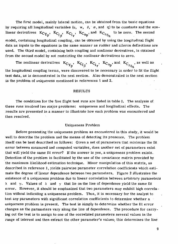
The first model, mainly lateral motion, can be obtained from the basic equationsby requiring all longitudinal variables (u, w, 9, a, and q) to be constants and the non-linear derivatives KCV , KQ , KQ , KQ , and K^ to be zero. The second
P £/3 ^r nP §amodel, containing longitudinal coupling, can be obtained by using the longitudinal flightdata as inputs to the equations in the same manner as rudder and aileron deflections areused. The third model, containing both coupling and nonlinear derivatives, is obtainedfrom the second model by not restricting the nonlinear derivatives to zero.
The nonlinear derivatives K^ , K(-. , KQ , KQ , and KQ , as well as
the longitudinal coupling terms, were discovered to be necessary in order to fit the flighttest data, as is demonstrated in the next section. Also demonstrated in the next sectionis the problem of uniqueness mentioned in references 1 and 2.
RESULTS
The conditions for the five flight test runs are listed in table I. The analysis ofthese runs involved two major problems: uniqueness and longitudinal effects. Theresults are presented in a manner to illustrate how each problem was encountered andthen resolved.
Uniqueness Problem
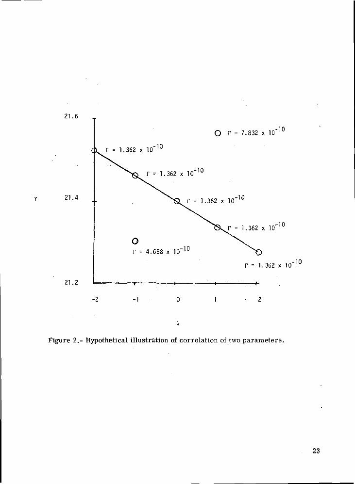
Before presenting the uniqueness problem as encountered in this study, it would bewell to describe the problem and the means of detecting its presence. The problemitself can be best described as follows: Given a set of parameters that minimize the fiterror between measured and computed variables, does another set of parameters existthat will yield the same fit error? If the answer is yes, a uniqueness problem exists.Detection of the problem is facilitated by the use of the covariance matrix provided bythe maximum likelihood estimation technique. Minor manipulation of this matrix, asdescribed in reference 1, yields pairwise parameter correlation coefficients which esti-mate the degree of linear dependence between two parameters. Figure 2 illustrates theexistence of a uniqueness problem due to linear correlation between arbitrary parametersX and y. Values of X and y that lie on the line of dependence yield the same fiterror. However, it should be emphasized that two parameters may exhibit high correla-tion without indicating a uniqueness problem. Thus, it is necessary for the analyst totest any parameters with significant correlation coefficients to determine whether auniqueness problem is present. The test is simply to determine whether the fit errorchanges as the parameters vary along the line of dependence. The procedure for carry-ing out the test is to assign to one of the correlated parameters several values in therange of interest and then extract the other parameter's values; this determines the line
of dependence. In figure 2, the fit error r does not change as A. and y vary alongthe line of dependence. Thus, a uniqueness problem is present. If the fit error didchange, both parameters would be identified by the estimation technique at the point ofminimum fit error and no uniqueness problem would exist, although the parameterswould still be correlated. In this hypothetical illustration, the correlation between Xand y is perfectly linear and will cause divergence of the estimation technique when anattempt is made to extract both parameters. However, in the use of real data, the pres-ence of noise usually prevents perfect linear correlation, and thus divergence.
Figure 3 presents the model responses generated by the estimates of the stabilityderivatives of test run 1 and the respective flight test data, using the first model with alllongitudinal variables fixed as constants (average values obtained from the flight data foreach variable). (Note that symbols in figure 3 and subsequent machine plots presentingmodel responses and respective flight test data are not the standard symbols defined inthe Symbols section.) Table II presents the estimates of the derivatives obtained, andtable in presents a form of the covariance matrix for these estimates. Diagonal ele-ments of this matrix are the standard deviations of the estimates, and the off-diagonalterms are correlation coefficients. As denoted by the asterisks of table in, Cyo, ^Yn'and CYr; C^, CZp, and C^; Cn/3, Cnp, and Cnr; and C^ and Cn/3 all have sig-
nificant correlation. Investigation of these parameters revealed the existence of a unique-ness problem.
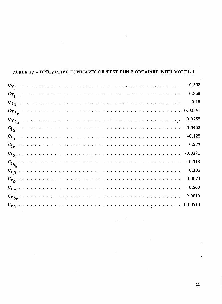
A major cause of uniqueness problems is generally admitted to be insufficientexcitation of the aircraft (for example, ref. 5). Test run 1 had rudder deflections only.Test run 2 contained both rudder and aileron deflections, and the model responses gener-ated by the derivative estimates for this test run and the respective flight test data areshown in figure 4. Again the longitudinal variables were fixed as constants during theextraction process. Table IV presents the estimates of the derivatives obtained, andtable V presents the modified covariance matrix. As pointed out in section 7.8.3 of ref-erence 5, the likelihood of obtaining a unique set of derivatives is increased when both arudder input and an aileron input are used to excite the airframe, as is evidenced by thelack of correlation exhibited in table V.
Longitudinal Coupling Effects
Examination of figure 4 (test run 2 responses) reveals poor fits for all the lateralvariables; these poor fits indicate a possibly incomplete model. The longitudinal datafor test run 2 are presented in figure 5 and indicate a substantial amount of longitudinalmotion. Use of the longitudinal data as input, together with the modeling of angle ofattack dependence of some of the derivatives, resulted in the extraction of a new set ofderivatives for test run 2. Figure 6 presents the model responses generated by this set
10
of derivatives and table VI contains the derivatives and their standard deviations. Nosignificant correlation was present and, thus, a unique set of derivatives has beenextracted. It should be noted that a lack of confidence exists for all the Cy deriva-tives with the exception of Cyo, due to the large standard deviations of the estimates,as is the case with some of the nonlinear derivatives.
Solution of the Uniqueness Problem
The uniqueness problem of test run 1 was resolved by fixing the values of the non-linear derivatives and (Cy A > C^ , and Cnr at the values obtained in test run 2
\ / Cc rri "
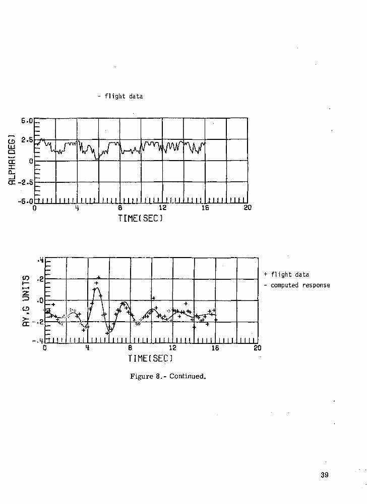
(the wind-tunnel results presented in ref. 4 show these derivatives to be fairly insensi-tive to Mach number variations in this flight regime) and extracting the remaining deriv-atives. This same procedure was used to solve the uniqueness problem of test run 3,which also had a rudder-only input. The model responses generated by the final esti-mates of the derivatives for test run 1 and test run 3 are shown with the respective flightdata in figures 7 and 8, respectively. The values of the derivatives and their standarddeviations are presented in table VII for test run 1 and table VIII for test run 3.
Test run 4 had essentially a rudder-only input, whereas test run 5 had both rudderand aileron inputs. Again, the results of test run 5 were used to solve the uniquenessproblem of test run 4. The model responses generated by the final derivative estimatesof test run 4 and the respective flight data are shown in figure 9, and the estimates withthe standard-deviations are presented in table IX. The results of test run 5 are presentedin figure 10 and table X.
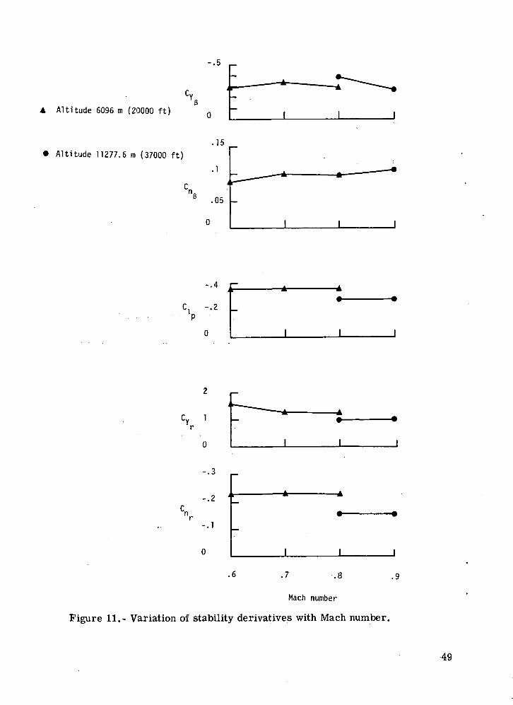
The total results of the analysis are summarized in figures 11 to 13, which illus-trate the variation of the extracted derivatives with Mach number, altitude, and angle ofattack. The results shown in figure 13 are presented with the intercept values locatedat the trim angle of attack (symbol location) and the slope of the lines determined by thenonlinear derivatives.
CONCLUDING REMARKS
It is believed that the importance of the analyst, exercising engineering judgmenttempered with estimator statistics, has been aptly demonstrated by the results of thisstudy in recognizing and resolving the problems of uniqueness and longitudinal couplingeffects. Thus, the extraction technique and its computer implementation have been shown
11
to provide the means for identifying both modeling and uniqueness problems and to yielda unique set of derivatives from actual lateral flight test data, provided the flight datacontain sufficient information.
Langley Research Center,National Aeronautics and Space Administration,
Hampton, Va., August 4, 1972.
REFERENCES
1. Grove, Randall D.; Bowles, Roland L.; and Mayhew, Stanley C.: A Procedure forEstimating Stability and Control Parameters From Flight Test Data by UsingMaximum Likelihood Methods Employing a Real-Time Digital System. NASATN D-6735, 1972.
2. Steinmetz, George G.; Parrish, Russell V.; and Bowles, Roland L.: Longitudinal Sta-bility and Control Derivatives of a Jet Fighter Airplane Extracted From FlightTest Data by Utilizing Maximum Likelihood Estimation. NASA TN D-6532, 1972.
3. Aiken, William S., Jr.: Standard Nomenclature for Airspeeds With Tables and Chartsfor Use in Calculation of Airspeed. NACA Rep. 837, 1946. (Supersedes NACATN 1120.)
4. Bonine, W. J.; Niemann, C. R.; Sonntag, A. H.; and Weber, W. B.: Model F/RF-4B-CAerodynamic Derivatives. Rep. 9842, McDonnell Aircraft Corp., Feb. 10, 1964.(Rev. Aug. 1, 1968.)
5. Wolowicz, Chester H.: Considerations in the Determination of Stability and ControlDerivatives and Dynamic Characteristics From Flight Data. AGARD Rep. 549-Pt. I,1966.
12
TABLE I.- FLIGHT TEST CONDITIONS
Testrun
12345
Altitude
m
6 0966 0966 096
11 277.611 277.6
ft
20 00020 00020 00037 00037 000
Machnumber
0.6.7.8.9.8
Center ofgravity,
% c
32.1931.8531.4929.1829.11
Input
RudderRudder and aileronRudderRudderRudder and aileron
TABLE II.- DERIVATIVE ESTIMATES OF TEST RUN 1 OBTAINED WITH MODEL 1
CYfl -0.392
-npCr
Cr
1.97
3.75
-0.0487
-0.0938
-0.355
-0.230
0.00221
0.120
0.162
-0.0664
0.0462
13
.
<o£
u
*H
~1— t V.J
jj
HpSj C«5 coEHj>r
p CQ.
g cf
^EHmO rH
<OTH r-O
(j i
PS"
EHCO *-
W (EH
rH
co aH 1*°H
§H „^^ f*-i"W owu2 ^ri o3 r**^ cOU
1
• "rH (>H
hH O
w,JPQ2 r*^M O
CQ_t^
CJ
CMCO
o
mooi
CDO
0
COooi
i— iTH
o1
c-oo
iH0o
CD0O
OJinoi
*TH
OSO
.£.
inOJo"
CDTHOJoo
CI
o
CM*1O
COTH
oi
COoo
inTH
o
mTH
oi
rH1— 1
o
COOo
THTH
o
CDmo
.£.
inOJ0
OJCDCD
O
*ineno
1 £
U
c-coo
c-oo
1
CMOo00
oo
1
inTH
o*1
COoo
mo0
CDoo
COCD
01
OJCOCO
TH
inOJ
o
.iHOJ
O
i- r
0
COOo1
oCO
o1
inCO
oi
CDCM*
O
inoo
CMi-H
O
in
o
COoo*
COCOoo
COCD
O1
CDinoi
OJinoi
H K
0
*ino
in°°.Oi
CMcoo
#THOJ
o1
o
01
*oOS
o
*
OJ
o
CM
COoo•o
cooo
CDoo"
THTH
o
CDoo
rH5 c
r-Ju
CMin0
^I>o
1
m£—0
1
CDl>0
1
CDinoi
*OJCO
o
S0
•*CMOJ
o
inrH
O
inoo
cooo
iHOC)
a sr>*
1in0
inCO
0i
coino
COinoi
OJinoi
COi— iCDOO
• *OJcoo
*ooso
CMrH
0
COoo
THTH
o"
t-oo
i r) ***$
U
co
oi
THrH
O
CMi— 1
O
CO1— 1
0
coCO1— 1oo0
OJmo
CDinoi
o
o1
ino0
inrH
O
inl-H
O1
rHrH
O1
4 <•
cT
CMCDO
1
•*
OS
o
•it-CDOJ*
O
OJir-rH0o0
COrH
O
coin0i
CDD-
OI
rH03
O
'
COCM
O1
^0o
1
mrH
oi
COoo
1
° cU
OJinoi
*CDOT
O
OSCMrHOo
•)(•CDO3>O
CMrH
O
COin0i
mc-o
1
CMCO
o1
mCO
o
CMOooo
cooo
1
COoo
u
OJCDo
CMCDCOoo
*CDOS
o
•it-
OS
0
rHrH
O
inCD
OI
t-
o
inCO
o'
oCO
0|
i>o1
COrH
O'
ino0i
O
CMCOCO0ooo
OSCDO
1
OJinoi
CMCD>
O
co• fo
1
.[
in*
o
CMin0
H4
ino
COoo
t-coo
CM
•O
CMCO
o
^ <CCO
.
c0• rH
rtr— 10)rHrHOO
"Srto*rH• rH
g)• rH
CO*
M)
14
TABLE IV.- DERIVATIVE ESTIMATES OF TEST RUN 2 OBTAINED WITH MODEL 1
Figure 10.- Model responses generated by final derivative estimates of test run 5with longitudinal data as input.
45
- flight data
801
•7*76OLU
^751Y—Lu
0726
701
-
- /
-
tl 1 1II II
r**1
\ M 1 M II
/•/"V
1 1 1 1
^_
II 1 1 II II III 1 1 1 1 1
-
—
-
1 1 if"
244.14
236.52
228.90
221 .28
213.66
OLU
120
en
W( F
T/S
EC
)
§ 8
o
g
-
-
-
tl 1 1
w—*^
1 1 1 1
V/
MM
A
1 1 1 1
\yv~v
MM
L
1 II 1 MM 1 1 1 1 II 1 1
-
—
-
Mir
36.57
18.28 _0LU
0 WDr:
-18.28 2
-36.57
•2fr
o •*LU(O
£ .0ocr
s--.2 l 1 1 1 1 1 1 i M i
\/
MM 1 1 II
.2
— .1cr8: .0cri—LU tn: -.1
,AW
=-
tl 1 1
tvMTW
1 1 1 1
^-^^\TV
1 1 II
y-vA
1 1 1 1
kv^Arv\
1 1 1 I
\v
1 1 1 1 1 1 1 1 1 1 1 1 1 1 1 1 1 1 1 16 12T I M E ( S E C )
Figure 10.- Continued.
16 20
46
- flight data
COUJa
a: -l
10
5
0
-5
10(
—
-u ,
^"
11 1 1 1 III
v/
MIL
/^
II 1 1
Y j-J • -
MM
"x.
MM Mi l MM Mi l MM3 4 8 12 IB 2
TIME(SEC)
.4
IO .P1—
- .0CD
>- g
-.4C
=
^
K
^ 1 1 1)MM
H
A
*Jr_
MMi
*^~
MMe
?K^B
MM\
-M->-*
1 1 1 11
1 1 1 12
1 1 1 11
1 1 1 16
1 1 1 12
+ flight data
- computed
response
0
TIME(SEC)
Figure 10.- Continued.
47
+ flight data(_) .0UJtorr\ ITCO UQCC
<H
-1.2
.2
~-x, . 1O -1LU
" nto .It-CDCE01
S"1
80
un•"k *iU0LL)
h-
*—
-80
r y
ti l l
-
*A! }
^111—
f+W-
E\
till
.\
-M
MM
JVMM
AlniMM
/
1 1 1 1
\X1 1 1 1
v/M M
^w- ^
MM
Af •
MM
\
MM
,-i
W
MM
*$
^
MM
f*
1 1 1 1
fe.
\
1 II 1
>M4-
1 1 1 1
1 1 1 1
1 II 1
1 1 1
II 1 1
1 II 1
MM
1 1 1 1
1 1 II
1 1 1 1
MM
II 1 1
—
—
=i \r
- compute
24.38
1O 1 QIc .13 __^
LJUJ
O co<!n
1O 1Q ^*-Id- 13
-24 .38
1.0
-. .5QCCK at— i
S -.5
-1.0I
-
- '^
t i l l
rf\
\
UN
/VINI
. -rfW*H^
MM
titijsc&
MM
4^
1 1 1 1 III 1 MM 1 1 1 1 1 1 1 1J 4 8 12 16 2
TIME(SEC)
Figure 10.- Concluded.
48
A Altitude 6096 m (20000 ft)
Altitude 11277.6 m (37000 ft).15
.1
.05
-.4 r-
0
.
-
1
A
1 1
-.3
-.1
0
.6
I
.7 .8
Mach number
Figure 11.- Variation of stability derivatives with Mach number.
.9
49
Altitude 6096 m(20000 ft)
Altitude 11277.6 m(37000 ft)
-.02
.1
.05
.1
V .05a
-.05
0
.6
I
.7
I
.9
Mach number
Figure 12.- Variation of control derivatives with Mach number.
50
Altitude 6096 m(20000 ft) r
Mach 0.6
Mach 0.7
Mach 0.8
Altitude 11277.6 m(37000 ft)
» Mach 0.8
O Mach 0.9
.4
.3
.2
.1
-.05
\ 0
-.3
.01
-.01
Figure 13.- Variation of parameters .with angle of attack.(Symbol at trim angle .of attack.)
NASA-Langley, 1973 2 L-8378 51
Le* Bla
NATIONAL AERONAUTICS AND SPACE ADMISTRATION
WASHINGTON. D.C'. '20546 .,',
OFFICIAL BUSINESS
PENALTY FOR PRIVATE USE $300FIRST CLASS MAIL
POSTAGE AND FEES PAID
NATIONAL AERONAUTICS AND
SPACE ADMINISTRATION
NASA 451
nncTM A CTCD . If Undeliverable (Section 1'.PUS I MASTER. posM| Manual) Do Not Re,
"The aeronautical and space activities of the United States shall beconducted so as to contribute . . . to the expansion of human knowl-edge of phenomena in the atmosphere and space. The Administrationshall provide for the widest practicable and appropriate disseminationof information concerning its activities and the results thereof."
— NATIONAL AERONAUTICS AND SPACE ACT OF 1958
NASA SCIENTIFIC AND TECHNICAL PUBLICATIONS
TECHNICAL REPORTS: Scientific andtechnical information considered important,complete, and a lasting contribution to existingknowledge.
TECHNICAL NOTES: Information less broadin scope but nevertheless of importance as acontribution to existing knowledge.
TECHNICAL MEMORANDUMS:Information receiving limited distributionbecause of preliminary data, security classifica-tion, or other reasons.
CONTRACTOR REPORTS: Scientific andtechnical information generated under a NASAcontract or grant and considered an importantcontribution to existing knowledge.
TECHNICAL TRANSLATIONS: Informationpublished in a foreign language consideredto merit NASA distribution in English.
SPECIAL PUBLICATIONS: Informationderived from or of value to NASA activities.Publications include conference proceedings,monographs, data compilations, handbooks,sourcebooks, and special bibliographies.
TECHNOLOGY UTILIZATIONPUBLICATIONS: Information on technologyused by NASA that may be of particukrinterest in commercial and other non-aerospaceapplications. Publications include Tech Briefs.,Technology Utilization Reports andTechnology Surveys.
Details on the availability of these publications may be obtained from:
SCIENTIFIC AND TECHNICAL INFORMATION OFFICE
NATIONAL AERONAUTICS AND SPACE ADMINISTRATIONWashington, D.C. 20546