LATTICE BOLTZMANN METHOD for CFDaeweb.tamu.edu/Richard/LBE9a.ppt.pdfLATTICE BOLTZMANN METHOD for CFD...

･ Department of Aerospace Engineering･

LATTICE BOLTZMANNMETHOD for CFD

More @ LBE

Dr. Jacques C. Richard, [email protected]. Sharath Girimaji, [email protected]

Dr. Dazhi Yu, [email protected]. Huidan Yu, [email protected]

12/1/2003


What makes up fluids Fluid made of small, individual molecules.

Molecules are in a state of constant motion.

Molecules are at continuous collision witheach other.

Molecule has internal structure.

There are intermolecular forces.

Macroscopic variables, such as pressure,temperature, and internal energy, are determinedby the mass, velocity, and internal structure ofmolecules.


Modeling FluidsKnudsen number

Microscopic Method : Molecular dynamics Kn<∞Mesoscopic Method : Boltzmann Equation Kn<∞Macroscopic Method: Navier-Stokes Equations Kn <0.1A Novel Method : Lattice Boltzmann Method Kn<0.1

�

Kn ! Mean free pathCharacteristic hydrodynamic length


Modeling of Fluids

BoltzmannEquation

MomentEquations

DiscreteVelocity model

Direct simulationMonte Carlo

Lattice BoltzmannEquation

Discretized phase-space & time

Kinetic Theory, Chapman-Enskog analysis

Navier Stokes Equations

microscopic

macroscopic

Taylor expansion in space and time


Velocity distribution function

Velocity distribution function: F(ci)

cdVPhysical space : ( x1, x2, x3 ) Velocity space: ( c1, c2, c3 )

ic

m : mass of molecule!N : number of molecules in !Vx

n(xi) : local number density

x2

x3

x1

xi

c2

ci

c3

c1

�

! = lim"Vx #0

m "N"Vx

= mn(xi)

�

F(ci) = lim!Vc "0

!N!Vc


Velocity Distribution Function

Normalized Velocity distribution Functionf(ci) = F(ci) / NN: Number of molecules in system

Characteristics of Distribution Function f 1.

2.

is the average value of Q for all moleculesMacrosopic velocity:

�

Nf (ci)dVc = N!"

"# $ f (ci)dVc =1!"

"#

�

Q =QdN

N!N

=Q(ci)Nf (ci)dVc"#

#!N

= QfdVc"#

#!

�

Q

�

r u = u = c = ci!"

"# fdVc


Velocity Distribution Function underEquilibrium State

Equilibrium State In equilibrium state, the number of molecules in ci is constant.

Distribution function under equilibrium state is theMaxwellian distribution:

T: temperature;k : Boltzmann constant (1.38054"10-16 erg-K)m: mass of moleculeu : macroscopic velocity

ic

�

f eq (ci) = m2!kT" # $

% & ' 3 / 2

e( m2kT

(c1(u1 )2 +(c2(u2 )

2 +(c3(u3 )2[ ]


Boltzmann Equation

Under non-equilibrium state distributionfunctionf = f(xi, ci, t) = f(x, c, t)

The molecular velocity distribution functionhas a rate of change, with respect to positionand time, that is described by

�

!!t

nf (ci)[ ] + c j!!x j

nf (ci)[ ] = !!t

nf (ci)[ ]" # $

% & ' collision


Collisions in fluids

Molecules constantly collide with each other.

Collision will change the velocity of molecules.

In collision, the translational energy of molecule may transferto internal energy, if molecule has internal structure.

In general, the rate of collision depends on the moleculevelocity, number density n(x), and temperature T.

zi

ci

zí

cí


Collision Operator in Boltzmann Equation Elastic-sphere molecule model

1. no internal structure of molecule,2. the molecule is treated as a rigid ball,3. so no rotation and vibration,4. only translation.

no attraction force between molecules.

Rigid elastic spheres

Repulsion

Attraction

True representation

d

r

∞

d: diameter of molecule; r: distance between molecules


Collision operator Rigid ball model gives:

g: relative velocity between two collided molecules

f(cí)f(zí): replenishing of the molecules of class ci

f(ci)f(zi) : depleting of the molecules of class ci

Integration limits: # from 0 to "/2 ; $ from 0 to 2".

Original collisionDepletion of ci and zi

zi

ci

zí

cí

zi

ci

zí

cí

Inverse collisionReplenishing of ci and zi

�

!!t

nf (ci)[ ]" # $

% & ' collision

= n2d2 f c'i( ) f z'i( ) ( f ci( ) f zi( )[ ]0

) / 2

* gsin+ cos+d+d,dVx0

2)

*(-

-

*


Macroscopic variables

Quantities of interest

Density

Momentum

Translational energy

�

! = mfdVc"#

#$

�

!u = mcfdVc"#

#$

�

etr = 12

c ! c ( )2 fdVc!"

"#


Moments of the Boltzmann Equation Let Q(ci) be a function of ci but not of position

and time, the equation of transfer of Q(ci) is

if Q=m, mci, mc2/2, the change in Q for bothmolecules must be zero in collision. We have

Let Q = m, we have the continuity equation in NS. We recover themomentum and energy equations in NS when Q=mci, mc2/2

�

Q(ci)!!t

nf (ci)[ ] + c j!!x j

nf (ci)[ ]" # $

% & ' dVc

()

)

* = Q(ci)!!t

nf (ci)[ ]" # $

% & ' collision

dVc()

)

*

�

!!t

nQ [ ] + !!x j

nQci[ ] = " Q[ ]

�

!!t

nQ [ ] + !!x j

nQci[ ] = 0


The Conservation Equations from theBoltzmann Equation

New definition: %ij = -[& CiCj - p 'ij] qj = & Cj C2

C = c - c

Kinetic theory: e = etr = C2/2 h = htr = etr + p/& = 5RT/2

& = nm p = &[C12 + C2

2 + C32 ]/3

tr: translational

Q = m

Q = mci

Q = mc2/2�

!"!t

+ !!x j

"c j( ) = 0

�

!!t

"c j( ) + !!xi

"c jc i( ) = # !p!x j

+!$ ij

!xi

�

!!t

" e + c 2( )[ ] + !!xi

"c i h + 12

c 2# $ %

& ' (

) * +

, - . =

!!xi

/ ijc k 0 qi( )


The Chapmen-Enskog Solution ofBoltzmann Equation

Non-dimensional form

cr: reference molecule speed ; L: characteristic length

vr: reference collision frequency

( = cr / L vr is proportional to the Knudsen #, the ratio of the meanfree path to a characteristic length, thus it is a very small value. Chapman-Enskog expansion (simplifying definitions ( ):

f(x, c, t) = f(eq)(x, c, t) + ( f(1)(x, c, t) + …Solve the f(l) , then we get the solution for f �

f = ˆ n ̂ f �

! ""ˆ t

ˆ n ̂ f [ ] + ˆ c j""ˆ x j

ˆ n ̂ f [ ]# $ %

& ' (

= ""ˆ t

ˆ n ̂ f [ ]# $ %

& ' ( collision


Chapman-Enskog Procedure

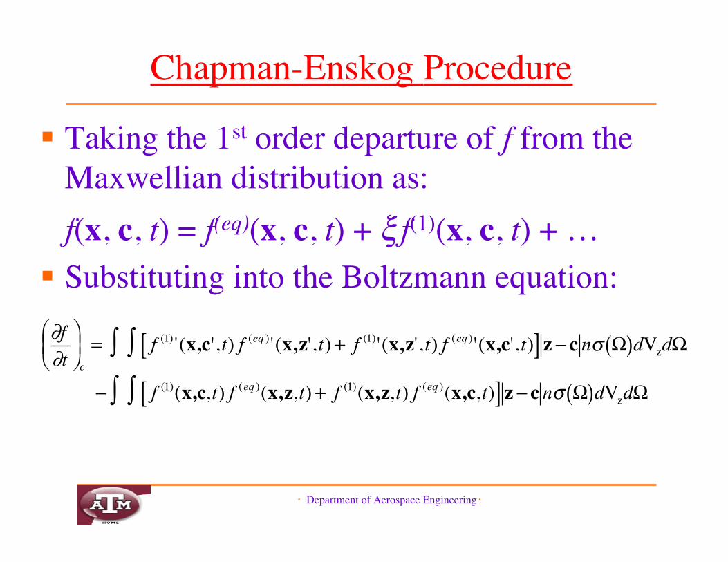
Taking the 1st order departure of f from theMaxwellian distribution as:f(x, c, t) = f(eq)(x, c, t) + ( f(1)(x, c, t) + …

Substituting into the Boltzmann equation:

�

!f!t

" # $

% & ' c

= f (1)'(x,c',t) f (eq )'(x,z',t) + f (1)'(x,z',t) f (eq )'(x,c',t)[ ] z ( c n) *( )dVzd*++( f (1)(x,c,t) f (eq )(x,z,t) + f (1)(x,z,t) f (eq )(x,c,t)[ ] z ( c n) *( )dVzd*++


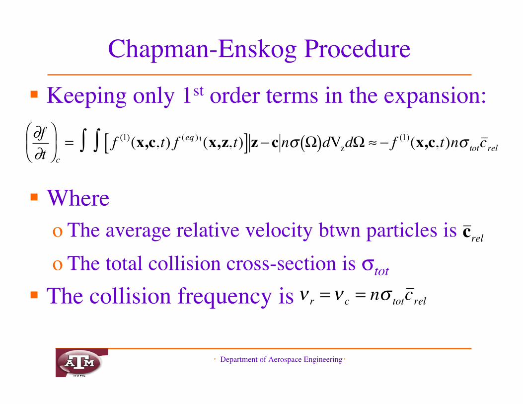
Chapman-Enskog Procedure Keeping only 1st order terms in the expansion:

Whereo The average relative velocity btwn particles iso The total collision cross-section is )tot

The collision frequency is

�

!f!t

" # $

% & '

c

= f (1)(x,c,t) f (eq )'(x,z,t)[ ] z ( c n) *( )dVzd*++ , ( f (1)(x,c,t)n) totc rel

�

c rel

�

! r = ! c = n" totc rel


The “1st Order” Boltzmann Equation

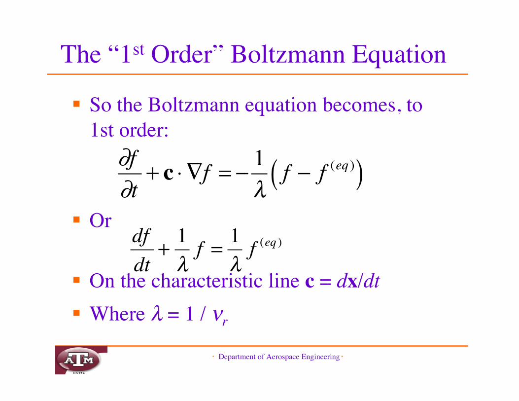
So the Boltzmann equation becomes, to1st order:

Or

On the characteristic line c = dx/dt Where * = 1 / +r

�

!f!t

+ c " #f = $ 1%

f $ f (eq )( )

�

dfdt

+ 1!f = 1

!f (eq )


Integrating the “1st Order” BE

Integrating the “1st Order” BE over a timestep 't:

Assuming 't is small enough & f(eq) issmooth enough locally, then for 0≤t’≤'t:

�

f (x + c!t ,c,t + !t ) = 1"e#! t /" et ' /" f (eq )(x + ct',c,t + t')dt'

0

! t$ + e#! t /" f (x,c,t)

�

f (eq )(x + ct',c,t + t') = 1! t'"t

#

$ %

&

' ( f (eq )(x,c,t) + t'

"tf (eq )(x + c"t ,c,t + "t ) + O "t

2( )


Integrating the “1st Order” BE

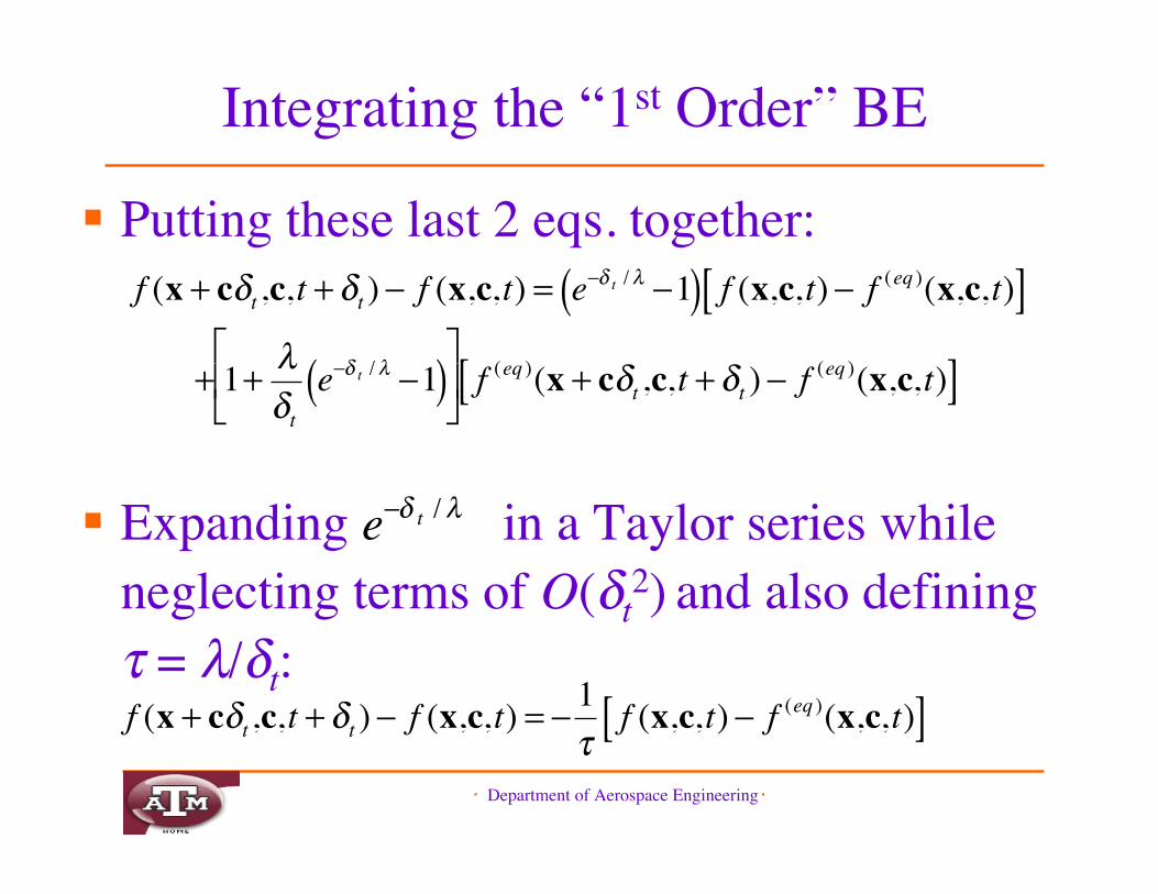
Putting these last 2 eqs. together:

Expanding in a Taylor series whileneglecting terms of O('t

2) and also defining% = */'t:

�

f (x + c!t ,c,t + !t ) " f (x,c,t) = e"! t /# "1( ) f (x,c,t) " f (eq )(x,c,t)[ ]+ 1+ #

!te"! t /# "1( )

$

% &

'

( ) f (eq )(x + c!t ,c,t + !t ) " f (eq )(x,c,t)[ ]

�

e!" t /#

�

f (x + c!t ,c,t + !t ) " f (x,c,t) = " 1#

f (x,c,t) " f (eq )(x,c,t)[ ]


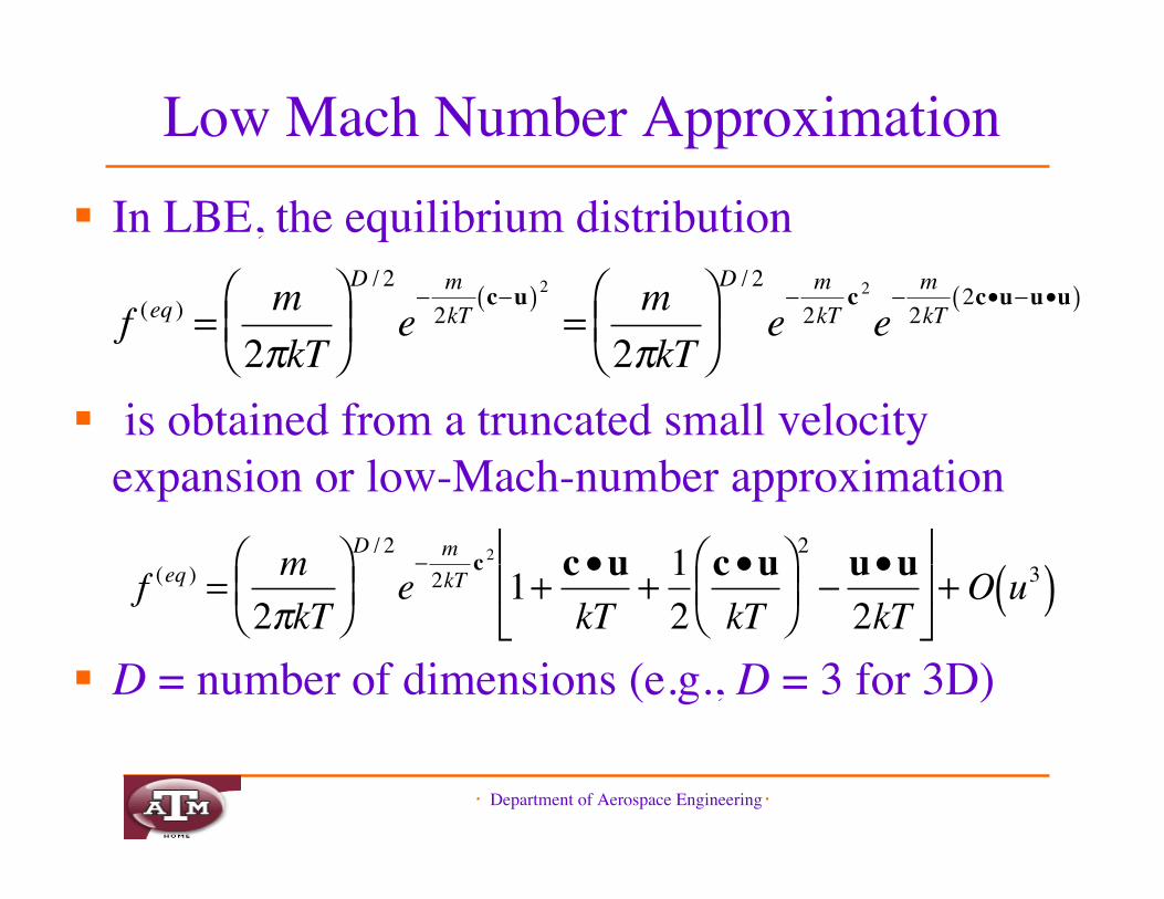
Low Mach Number Approximation In LBE, the equilibrium distribution

is obtained from a truncated small velocityexpansion or low-Mach-number approximation

D = number of dimensions (e.g., D = 3 for 3D)

�

f (eq ) = m2!kT

" # $

% & ' D / 2

e( m2kT

c(u( )2= m2!kT" # $

% & ' D / 2

e( m2kT

c 2e( m2kT

2c•u(u•u( )

�

f (eq ) = m2!kT" # $

% & ' D / 2

e( m2kT

c 21+ c •u

kT+ 12c •ukT

" # $

% & ' 2

( u•u2kT

)

* +

,

- . + O u3( )


Discretization of Phase Space Discretization of momentum space is

coupled to that of configuration space suchthat a lattice structure is obtained

This is a special characteristic of LBE Quadrature must be accurate enough to

• Preserve conservation constraints exactly• Retain necessary symmetries of Navier-Stokes


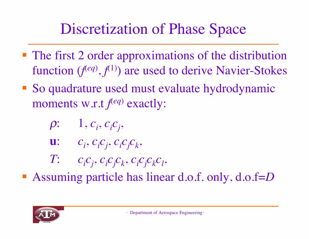
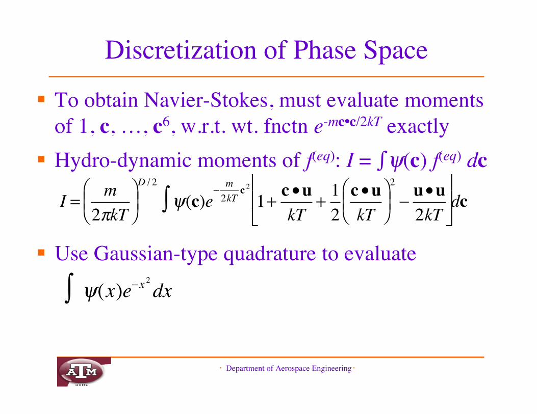
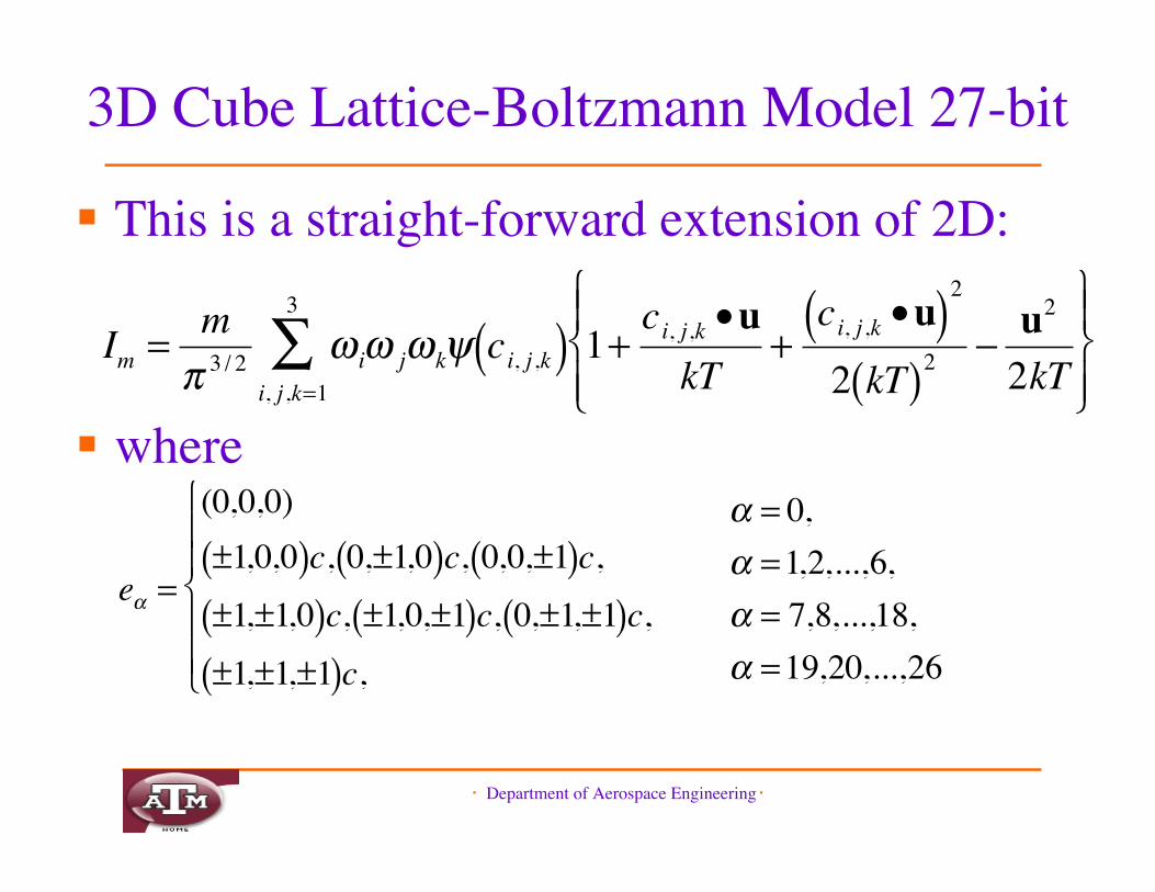
Discretization of Phase Space The first 2 order approximations of the distribution

function (f(eq), f(1)) are used to derive Navier-Stokes So quadrature used must evaluate hydrodynamic

moments w.r.t f(eq) exactly:&: 1, ci, cicj,u: ci, cicj, cicjck,T: cicj, cicjck, cicjckcl,

Assuming particle has linear d.o.f. only, d.o.f=D


Discretization of Phase Space

To obtain Navier-Stokes, must evaluate momentsof 1, c, …, c6, w.r.t. wt. fnctn e-mc•c/2kT exactly

Hydro-dynamic moments of f(eq): I = ∫ #(c) f(eq) dc

Use Gaussian-type quadrature to evaluate

�

I = m2!kT" # $

% & ' D / 2

((c)e) m2kT

c 21+ c •u

kT+ 12c •ukT

" # $

% & ' 2

) u•u2kT

*

+ ,

-

. / 0 dc

�

!(x)e"x2dx#


Square Lattice-Boltzmann Model 9-bit 2D

In Cartesian coordinates: Then

Where

�

!mn (c) = cxmcy

n

�

I = !mn (c) f (eq )dc"#

#

$ = m%

2kT( )m+n&

1" u2

2kT'

( )

*

+ , ImIn +

2 uxIm+1In + uyImIn+1( )2kT

+ux2Im+2In + 2uxuyIm+1In+1 + ux

2ImIn+2

RT

- . /

0 /

1 2 /

3 /

�

Im = e!"2" md" ,

!#

#

$ " = c/ 2kT


Square Lattice-Boltzmann Model 9-bit 2D Use 3rd order Hermite formula to evaluate

Where the 3 abscissas of the quadrature are:

And the corresponding weight coefficientsare:

�

Im = e!"2" md"

!#

#

$ = % j" jm

j=1

3

&

�

!1 = " 3/2, ! 2 = 0, ! 3 = 3/2

�

!1 = " /6, !2 = 2 " /3, !3 = " /6


Moment integral becomes

From which, parts of the equilibriumdistribution function are identified as

�

Im = m!

" i" j# ci, j( ) 1+ci, j •ukT

+ci, j •u( )22 kT( )2

$ u2

2kT

% & '

( '

) * '

+ ' i, j=1

3

,

�

fi, j(eq ) = m

!" i" j 1+

ci, j •ukT

+ci, j •u( )22 kT( )2

# u2

2kT

$ % &

' &

( ) &

* &

2D Square Lattice-Boltzmann Model 9-bit


Select possible molecular velocities on 2D squarelattice to go in as many directions of such square

The chosen velocities have a certain symmetry toaccount for molecules moving in any and alldirections independent of directions (isotropy)

For square this means sides & corners This means 9 possible velocities To go w/at least 9 terms in #mn(c) 1

2 3 4

7

e2 e 3

e1

e4

e5

e6e7 e8

5

6 8


2

3

4

56

7


The 9 possible velocities are:

�

e! =(0,0),cos"! ,sin"!( )c,2 cos"! ,sin"!( )c,

"! = (! #1)$ /2,"! = (! # 5)$ /2 + $ /4,

! = 0,! =1,2,3,4,! = 5,6,7,8

%

& '

( '


1

2 3 4

7

e2 e 3

e1

e4

e5

e6e7 e8

5

6 8

2

3

4

56

7


2D Square Lattice-Boltzmann Model 9-bit Then parts of the equilibrium distribution function are

identified as

Where the corresponding weight coefficients are now

And RT = cs2 = c2/3 or

�

f!(eq ) = mw! 1+ e! •u

c 2+e! •u( )22c 4

" u2

2c 2# $ %

& %

' ( %

) %

�

w! =" i" j

#=4 /9,1/9,1/36,

i = j = 2,i =1, j = 2,...,i = j =1,

! = 0,! =1,2,3,4,! = 5,6,7,8

$ % &

' &

�

RTr ! = 3RT = c


This is a straight-forward extension of 2D:

where

�

Im = m! 3 / 2 " i" j"k# ci, j ,k( ) 1+

ci, j,k •ukT

+ci, j ,k •u( )22 kT( )2

$ u2

2kT

% & '

( '

) * '

+ ' i, j ,k=1

3

,

�

e! =

(0,0,0)±1,0,0( )c, 0,±1,0( )c, 0,0,±1( )c,±1,±1,0( )c, ±1,0,±1( )c, 0,±1,±1( )c,±1,±1,±1( )c,

! = 0,! =1,2,...,6,! = 7,8,...,18,! =19,20,...,26

"

# $ $

% $ $

3D Cube Lattice-Boltzmann Model 27-bit


3D Cube Lattice-Boltzmann Model 27-bit

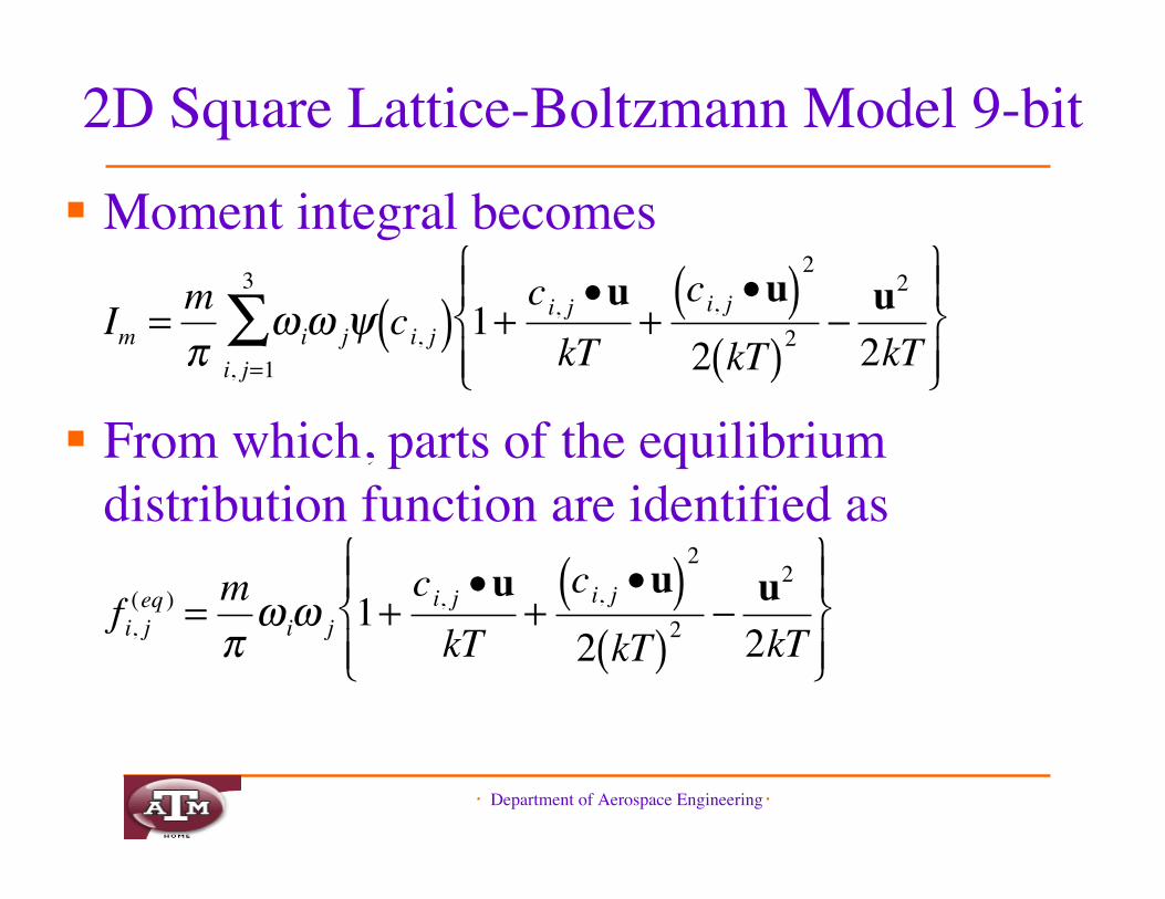
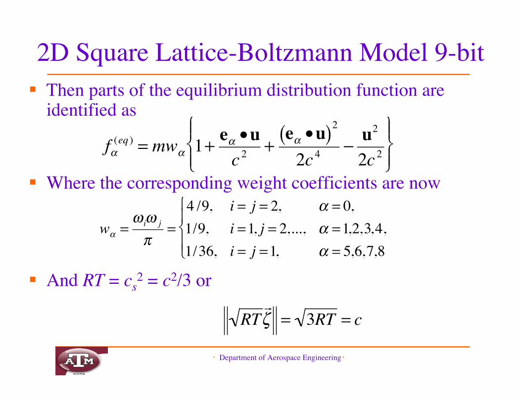
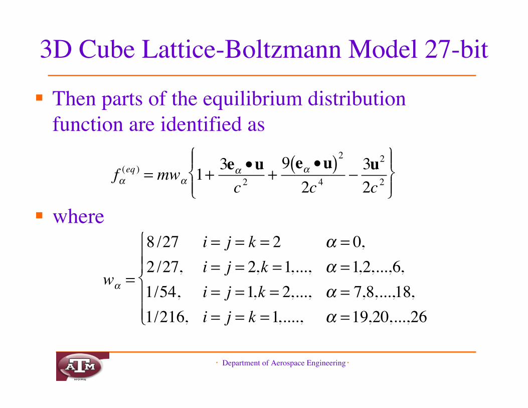
Then parts of the equilibrium distributionfunction are identified as

where

�

f!(eq ) = mw! 1+ 3e! •u

c 2+9 e! •u( )22c 4

" 3u2

2c 2# $ %

& %

' ( %

) %

�

w! =

8 /272 /27,1/54,1/216,

i = j = k = 2i = j = 2,k =1,...,i = j =1,k = 2,...,i = j = k =1,....,

! = 0,! =1,2,...,6,! = 7,8,...,18,! =19,20,...,26

"

# $ $

% $ $


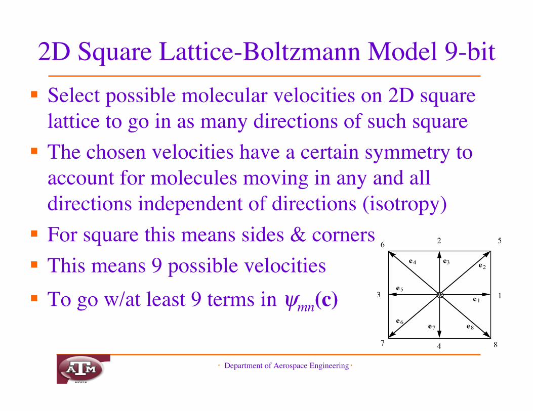
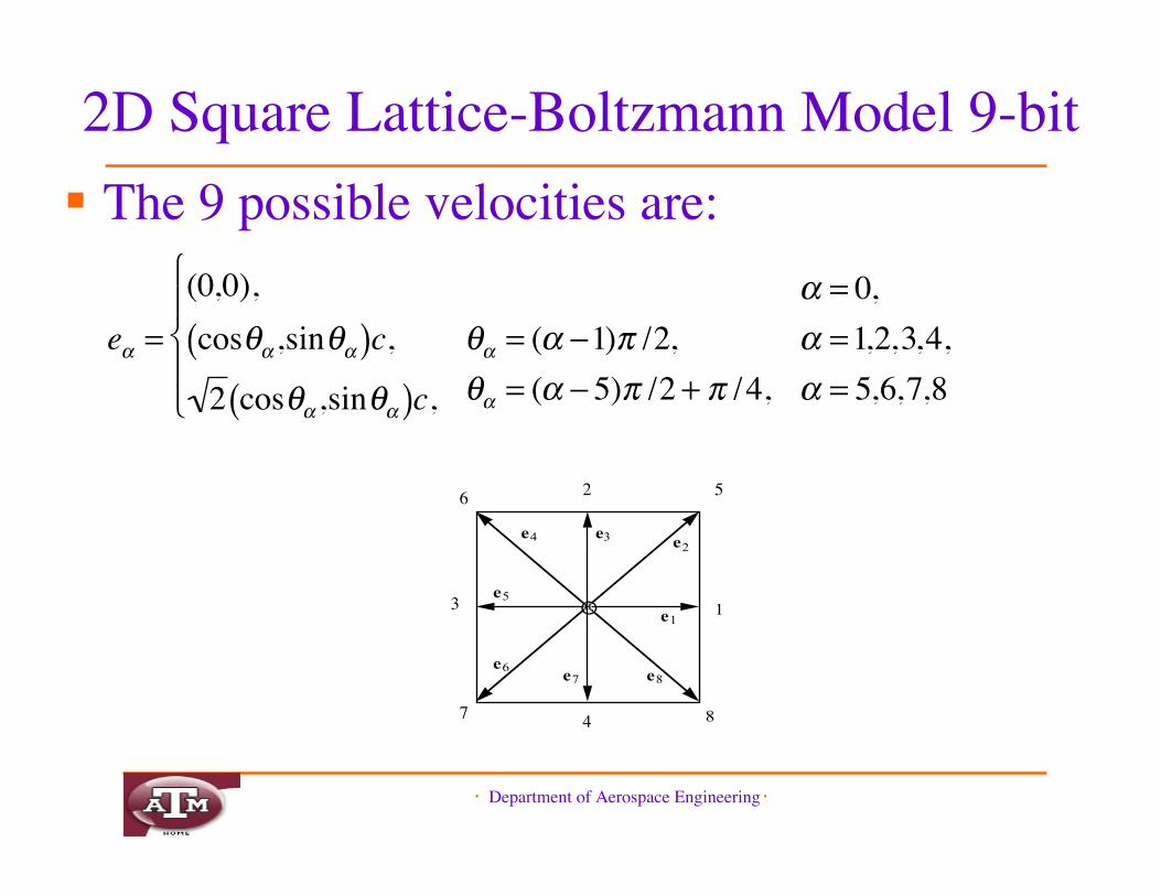
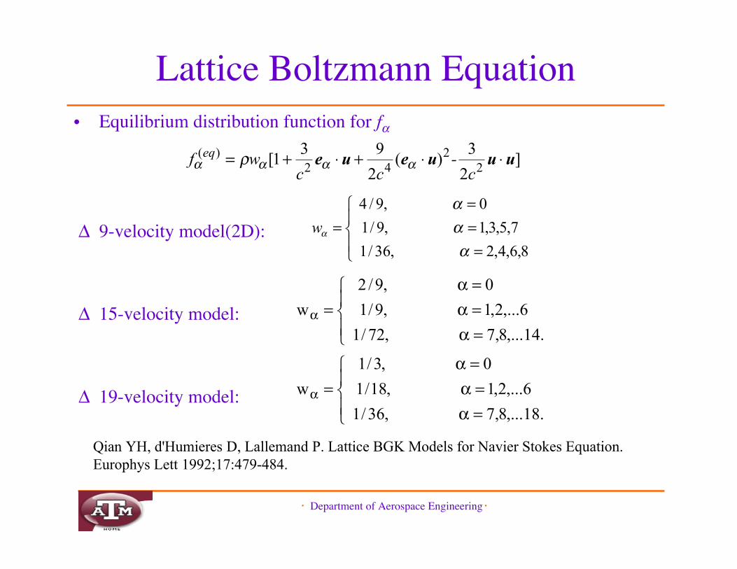
• Equilibrium distribution function for f,

! 9-velocity model(2D):

! 15-velocity model:

! 19-velocity model:

!"

!#$

=%=%=%

=%.14,...8,7,72/1

6,...2,1,9/1

0,9/2

w

]2

3)(

2

931[

22

42)( uuueue !!+!+=

c-

ccwf eq """" #

!"

!#$

=%=%=%

=%.18,...8,7,36/1

6,...2,1,18/1

0,3/1

w

Lattice Boltzmann Equation

Qian YH, d'Humieres D, Lallemand P. Lattice BGK Models for Navier Stokes Equation.Europhys Lett 1992;17:479-484.

!"

!#$

===

=8,6,4,2 ,36/1

7,5,3,1 ,9/1

0 ,9/4

%%%

%w


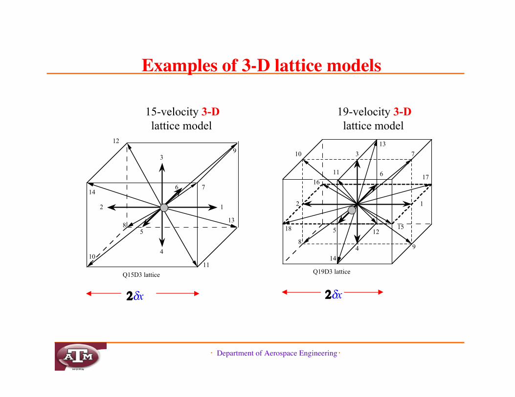
Examples of 3-D lattice models

2'x

6

8

7

9

1011

12

2 1

4

3

5

14

13

Q15D3 lattice

19-velocity 3-D lattice model

5

6

8

7

9

10

11

1215

1617

2 1

4

3

13

18

14

Q19D3 lattice

15-velocity 3-D lattice model

2'x


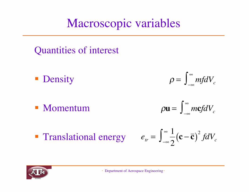
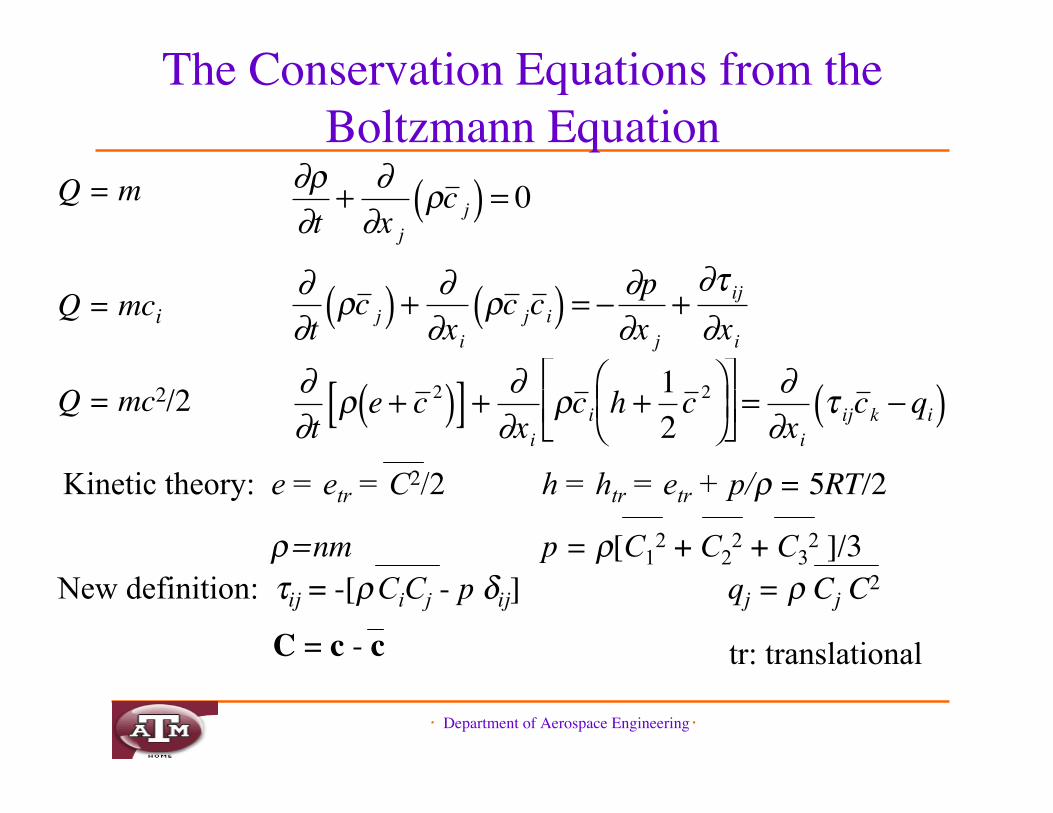
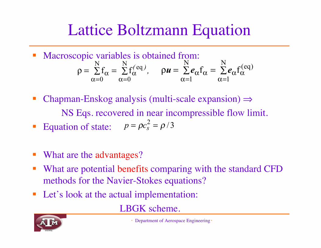
Macroscopic variables is obtained from:

Chapman-Enskog analysis (multi-scale expansion) -NS Eqs. recovered in near incompressible flow limit.

Equation of state:

What are the advantages? What are potential benefits comparing with the standard CFD

methods for the Navier-Stokes equations? Let’s look at the actual implementation:

LBGK scheme.

,)(!=!="=#

#=#

#N

0

eqN

0ff !=!="

=###

=###

N

1

)eq(N

1ff eeu

3/2 !! == scp



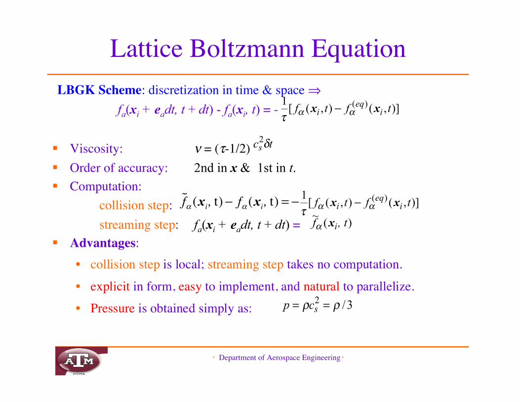
LBGK Scheme: discretization in time & space - fa(xi + eadt, t + dt) - fa(xi, t) = -

Viscosity: + = (%-1/2) Order of accuracy: 2nd in x & 1st in t. Computation:

collision step:streaming step: fa(xi + eadt, t + dt) =

Advantages:• collision step is local; streaming step takes no computation.• explicit in form, easy to implement, and natural to parallelize.• Pressure is obtained simply as:

)],(),([1 )( tftf i

eqi xx !!"

#

tcs!2

�

˜ f ! (xi, t) " f! (xi, t) = ")(

~, tf ix!

3/2 !! == scp


)],(),([1 )( tftf i

eqi xx !!"

#


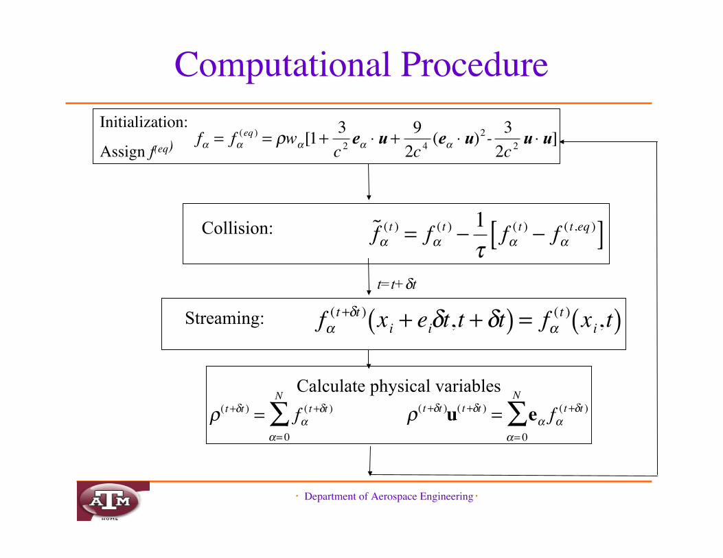
Collision:

Computational Procedure

Streaming:

t=t+'t

Calculate physical variables

�

˜ f !(t ) = f!

(t ) " 1#

f!( t ) " f!

( t,eq )[ ]

�

f!(t+"t ) xi + ei"t,t + "t( ) = f!

(t ) xi,t( )

�

!(t+"t ) = f#( t+"t )

#= 0

N

$

�

!(t+"t )u( t+"t ) = e# f#(t+"t )

#= 0

N

$

�

f! = f!(eq ) = "w![1+ 3

c 2e! # u + 9

2c 4(e! # u)2- 3

2c 2u # u]

Initialization:

Assign f(eq)


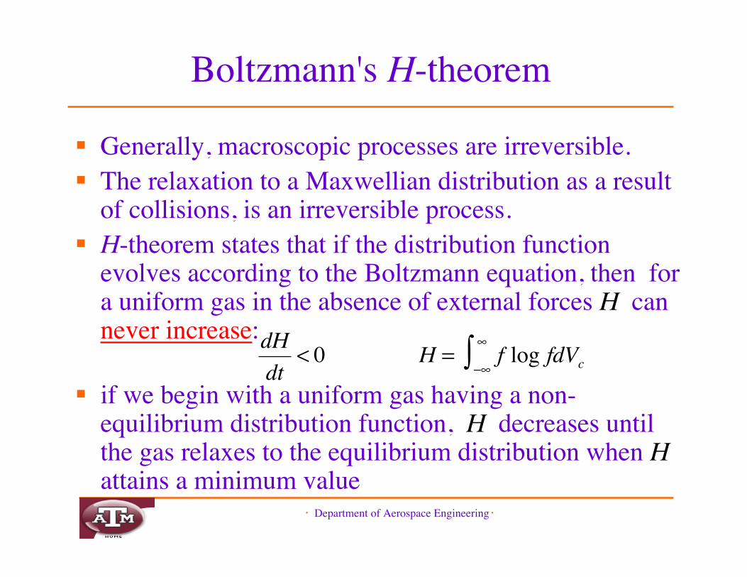
Boltzmann's H-theorem

Generally, macroscopic processes are irreversible. The relaxation to a Maxwellian distribution as a result

of collisions, is an irreversible process. H-theorem states that if the distribution function

evolves according to the Boltzmann equation, then fora uniform gas in the absence of external forces H cannever increase:

if we begin with a uniform gas having a non-equilibrium distribution function, H decreases untilthe gas relaxes to the equilibrium distribution when Hattains a minimum value�

dHdt

< 0

�

H = f log fdVc!"

"#


Applications of LBE Simulation of incompressible flows

Fully compressible and thermal flows

Multi-phase and multi-component flows

Particulate Suspensions

Turbulent Flows

Micro Flows


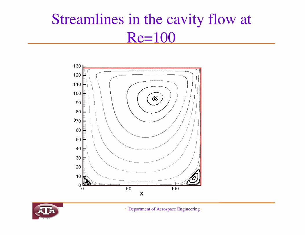
Streamlines in the cavity flow atRe=100

X

Y

0 50 1000

10

20

30

40

50

60

70

80

90

100

110

120

130


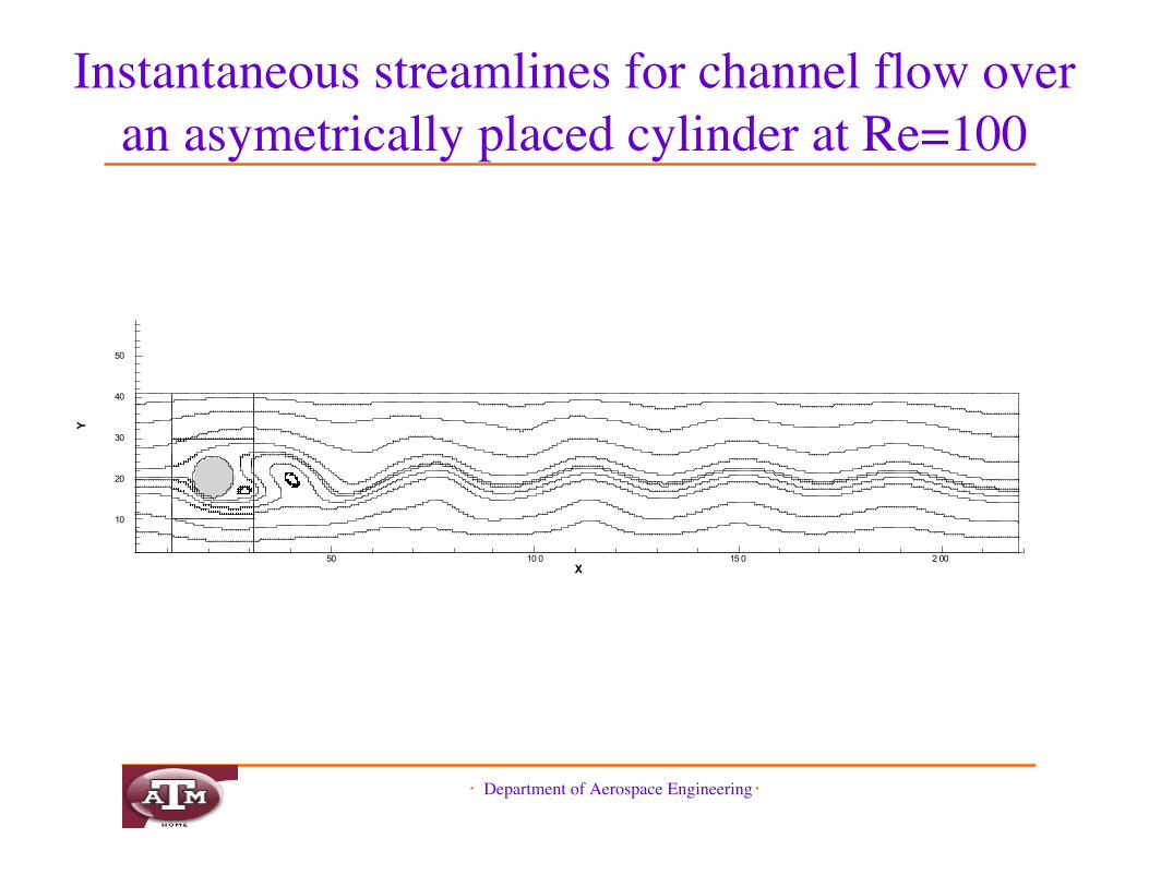
Instantaneous streamlines for channel flow overan asymetrically placed cylinder at Re=100

X

Y

50 10 0 15 0 2 00

10

20

30

40

50


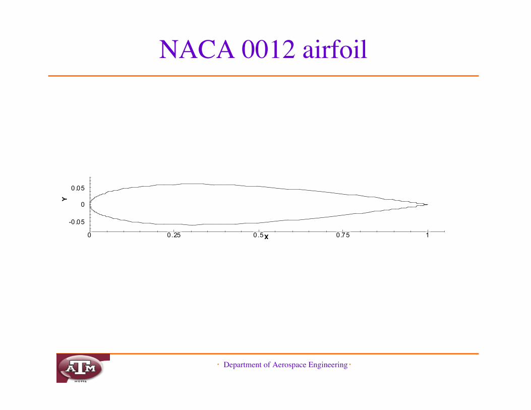
NACA 0012 airfoil

X

Y

0 0.25 0.5 0.75 1

-0.05

0

0.05


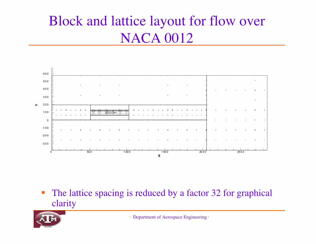
Block and lattice layout for flow overNACA 0012

The lattice spacing is reduced by a factor 32 for graphicalclarity

X

Y

0 50 0 1 00 0 1 50 0 20 0 0 25 0 0

-3 0 0

-2 0 0

-1 0 0

0

1 0 0

2 0 0

3 0 0

4 0 0

5 0 0

6 0 0


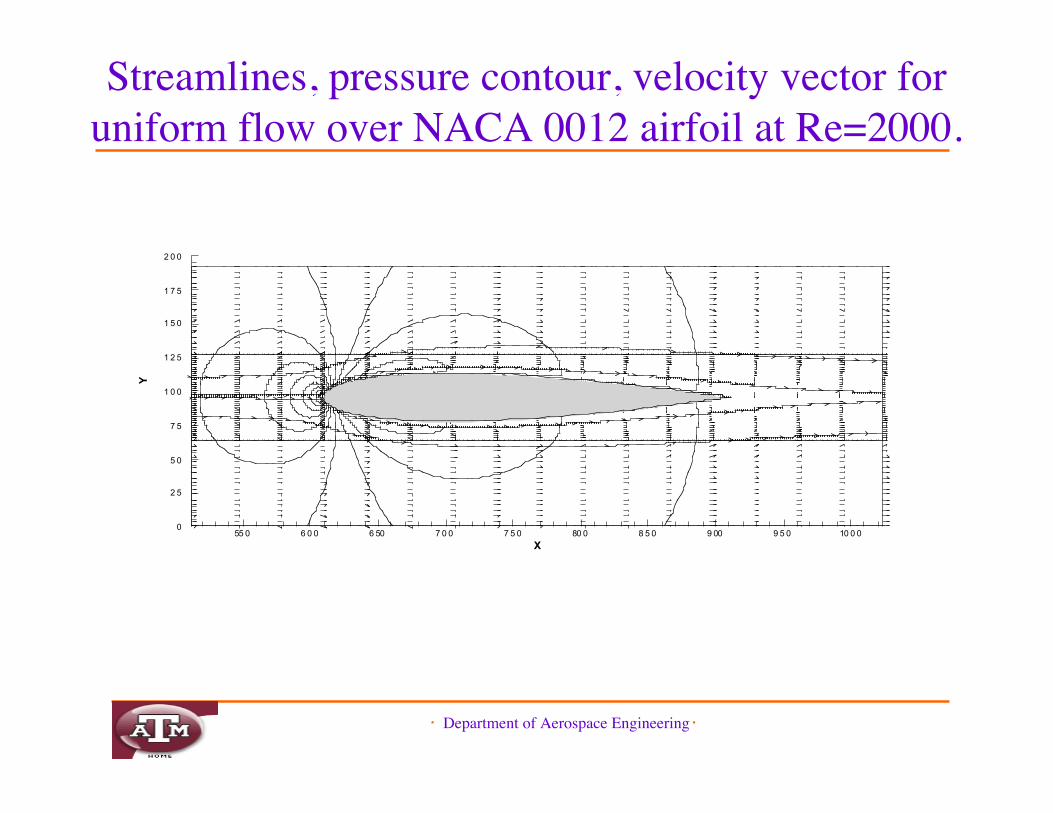
Streamlines, pressure contour, velocity vector foruniform flow over NACA 0012 airfoil at Re=2000.

X

Y

55 0 6 0 0 6 50 7 0 0 7 5 0 80 0 8 5 0 9 00 9 5 0 10 0 00

2 5

5 0

7 5

1 0 0

1 2 5

1 5 0

1 7 5

2 0 0


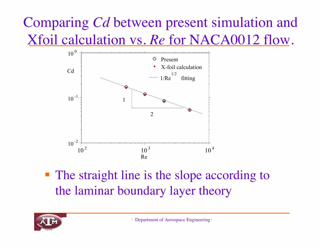
Comparing Cd between present simulation andXfoil calculation vs. Re for NACA0012 flow.

10 410 310 210 -2

10 -1

10 0

Present

1/Re fitting

X-foil calculation

Re

Cd

1

2

1/2

The straight line is the slope according tothe laminar boundary layer theory


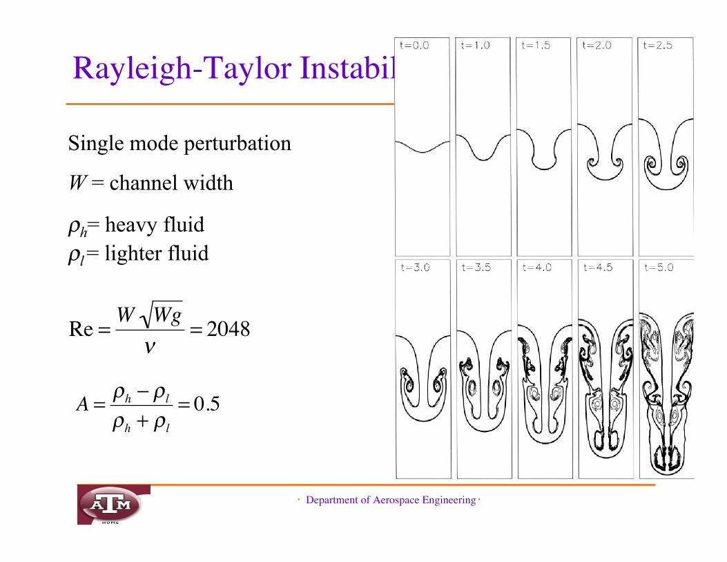
Rayleigh-Taylor Instability

Single mode perturbation

W = channel width

&h= heavy fluid&l = lighter fluid

�

Re = W Wg!

= 2048

�

A = !h " !l

!h + !l

= 0.5


Implementation of complex LBE model.

For complicated problems, new LBEmodels may need to be designed.

The number of particle velocities innew models can vary.

Hybrid modes which incorporatefinite different method in LBE needto be considered.


References for LBEMcNamara G, Zanetti G. Use of the Boltzmann equation to simulate lattice-gas automata. PhysRev Lett 1988; 61: 2332 –2335.

Higuera FJ, Jemenez J. Boltzmann approach to lattice gas simulations. Europhys Lett1989;9:663-668.

Koelman JMVA. A simple lattice Boltzmann scheme for Navier-Stokes fluid flow. EurophysLett 1991;15:603-607.

Qian YH, d'Humieres D, Lallemand P. Lattice BGK Models for Navier Stokes Equation.Europhys Lett 1992;17:479-484.

Chen H, Chen S, Matthaeus WH. Recovery of the Navier-Stokes equations using a lattice-gasBoltzmann method. Phys Rev A 1992;45:R5339-R5342.

d’Humieres D. Generalized lattice Boltzmann equations, In Rarefied Gas Dynamics: Theory andSimulations, ed. by D. Shizgal and D.P. Weaver. Prog. in Astro. Aero. 1992;159:450-458.

Bhatnagar PL, Gross EP, Krook M. A model for collision processes in gases, I. small amplitudeprocesses in charged and neutral one-component system. Phys Rev 1954;94:511-525.

He X, Luo L-S. A priori derivation of the lattice Boltzmann equation. Phys Rev E1997;55:R6333-R6336.

He X, Luo L-S. Theory of the lattice Boltzmann equation: From Boltzmann equation to latticeBoltzmann equation. Phys Rev E 1997;56:6811-6817.


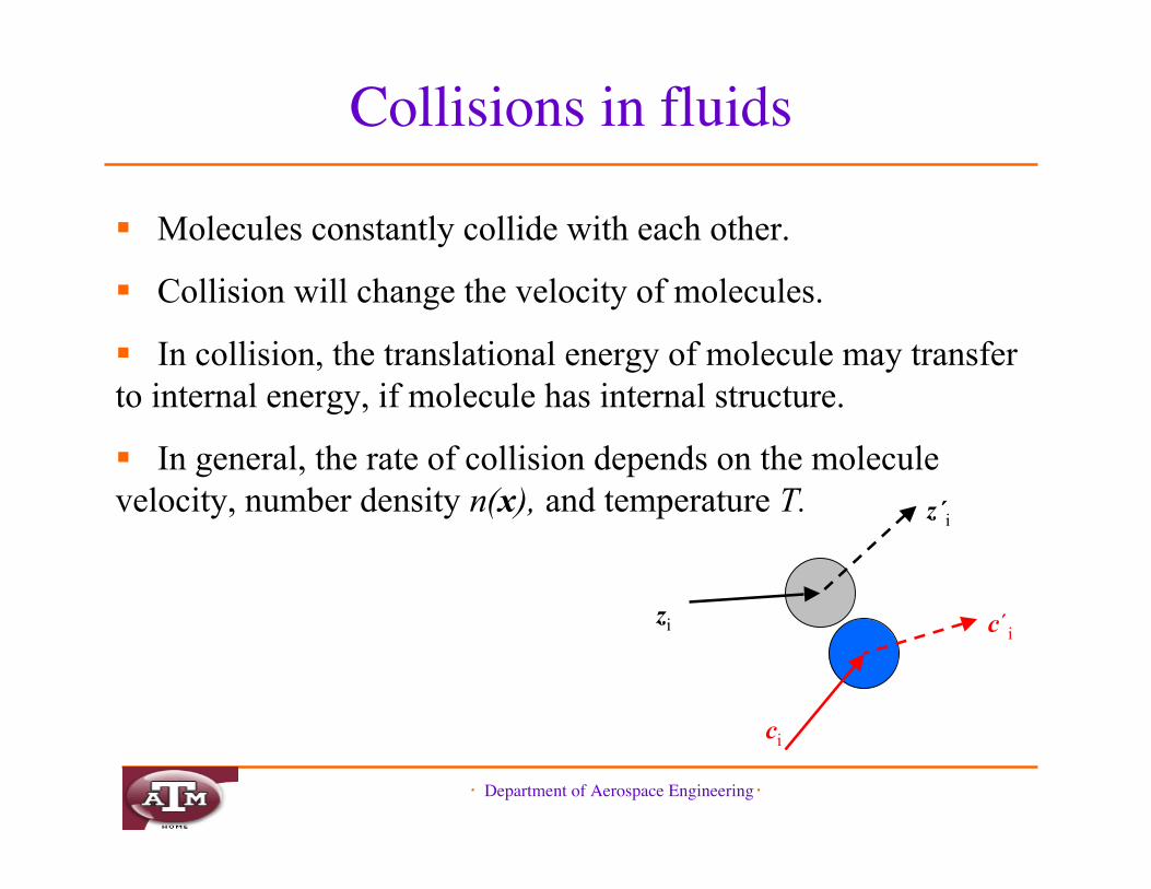
Boltzmann Equation

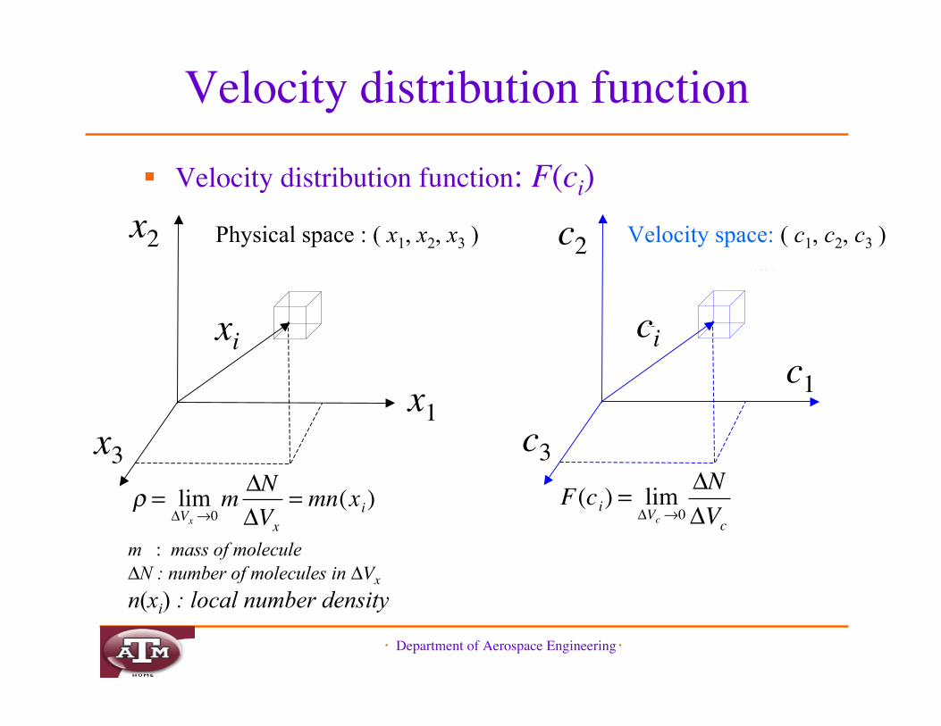
Studying molecules (class ci) inside dVx, wesee total number of molecules whose velocityis between ci and ci + dVc isnf(ci) dVx dVc

Change of number of molecules in class cimust result from convection of moleculesacross the surface of dVc and dVx or fromintermolecular collision within


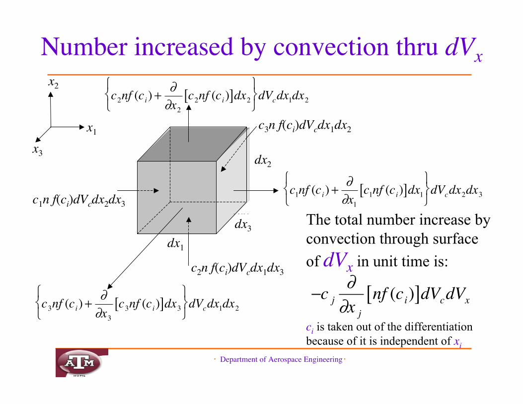
Number increased by convection thru dVx

1dx

3dxThe total number increase byconvection through surface

of dVx in unit time is:

ci is taken out of the differentiationbecause of it is independent of xi

x2

x1

x3

dx1

dx3

dx2

c3n f(ci)dVcdx1dx2

c1n f(ci)dVcdx2dx3

�

c2nf (ci) + !!x2

c2nf (ci)[ ]dx2" # $

% & ' dVcdx1dx2

�

c1nf (ci) + !!x1

c1nf (ci)[ ]dx1" # $

% & ' dVcdx2dx3

�

c3nf (ci) + !!x3

c3nf (ci)[ ]dx3" # $

% & ' dVcdx1dx2

c2n f(ci)dVcdx1dx3

�

!c j""x j

nf (ci)[ ]dVcdVx


Boltzmann Equation

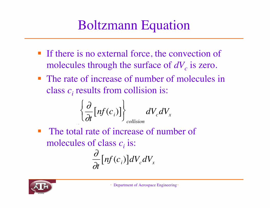
If there is no external force, the convection ofmolecules through the surface of dVc is zero.

The rate of increase of number of molecules inclass ci results from collision is:

The total rate of increase of number ofmolecules of class ci is:

ic

�

!!t

nf (ci)[ ]" # $

% & ' collision

dVcdVx

�

!!t

nf (ci)[ ]dVcdVx


Boltzmann Equation

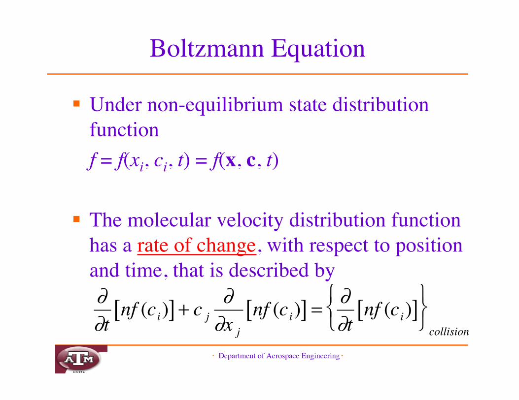
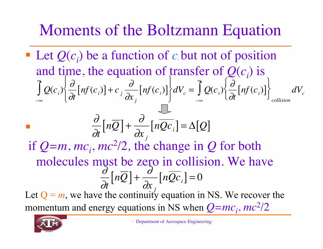
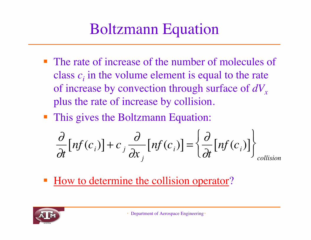
The rate of increase of the number of molecules ofclass ci in the volume element is equal to the rateof increase by convection through surface of dVxplus the rate of increase by collision.

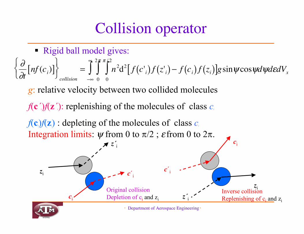
This gives the Boltzmann Equation:

How to determine the collision operator?

xdV

�

!!t

nf (ci)[ ] + c j!!x j

nf (ci)[ ] = !!t

nf (ci)[ ]" # $

% & ' collision


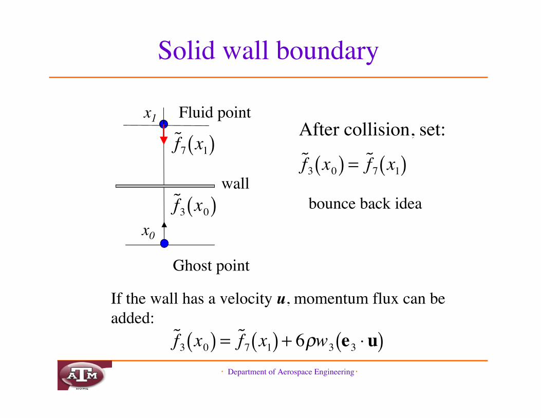
Solid wall boundary

Ghost point

wall

x1

x0

Fluid pointAfter collision, set:

bounce back idea

If the wall has a velocity u, momentum flux can beadded:

�

˜ f 7 x1( )

�

˜ f 3 x0( )

�

˜ f 3 x0( ) = ˜ f 7 x1( )

�

˜ f 3 x0( ) = ˜ f 7 x1( ) + 6!w3 e3 "u( )


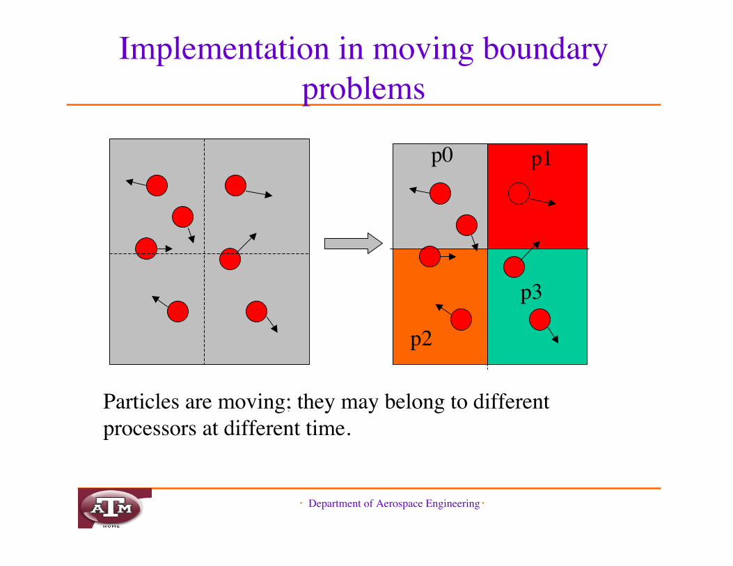
Implementation in moving boundaryproblems

p0 p1

p2

p3

Particles are moving; they may belong to differentprocessors at different time.


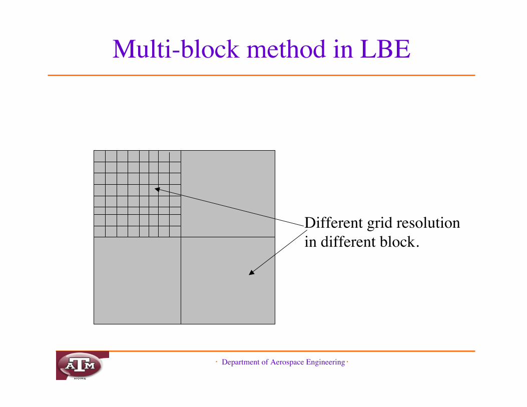
Multi-block method in LBE

Different grid resolutionin different block.


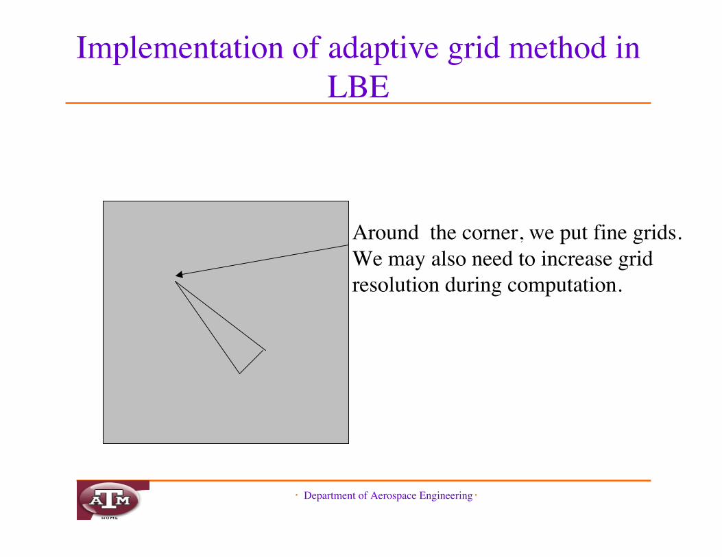
Implementation of adaptive grid method inLBE

Around the corner, we put fine grids.We may also need to increase gridresolution during computation.


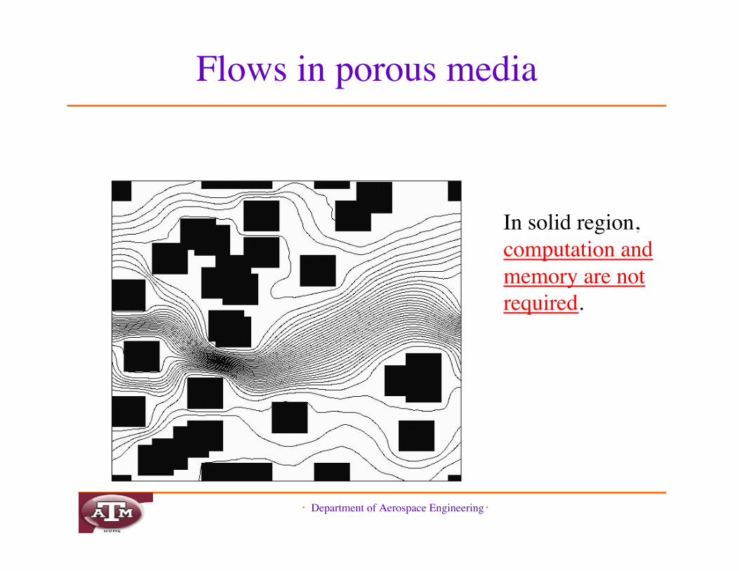
Flows in porous media

In solid region,computation andmemory are notrequired.


Boltzmann’s H Theorem Generally, entropy, S, is defined to be related to the

# of possible arrangements of molecules In other words, entropy is a function of # of

possible micro-states, . The probability distribution function provides a

way of determining the # of possible macro-states, Because . for combined systems of certain micro-

states is a product of each, .AB = .A .B And because total entropy is SAB = SA + SB

S = - k log . = - k ∫ f log f dVc,


Boltzmann’s H Theorem Differentiating H, using Boltzmann’s eq., & combining

terms:

H theorem shows why entropy is automatically satisfied ifBoltzmann’s eq. is satisfied

Many CFD schemes do not easily guarantee that they willnot violate entropy

Through solving BE,• entropy is inherently & automatically satisfied and• fluid field is found from f rather than using f to find properties to

use in Navier-Stokes eqs. derived from BE

�

dHdt

= ! 14

f (c') f (z') ! f (c) f (z)[ ] log f (c) f (z)f (c') f (z')

c ! z"d#dVz$$ % 0

Date post:	18-May-2018
Category:	Documents
Upload:	trantruc
View:	216 times
Download:	0 times

LATTICE BOLTZMANN METHOD for CFDaeweb.tamu.edu/Richard/LBE9a.ppt.pdfLATTICE BOLTZMANN METHOD for CFD...

Documents