Page 1
arX
iv:c
ond-
mat
/050
6768
v1 [
cond
-mat
.sof
t] 2
9 Ju
n 20
05
Lattice-Boltzmann Method for Non-Newtonian Fluid Flows
Susana Gabbanelli
Departamento de Matematica y Grupo de Medios Porosos,
Facultad de Ingenierıa, Universidad de Buenos Aires
German Drazer∗ and Joel Koplik†
Benjamin Levich Institute and Department of Physics,
City College of the City University of New York, New York, NY 10031
(Dated: October 30, 2018)
Abstract
We study an ad hoc extension of the Lattice-Boltzmann method that allows the simulation of
non-Newtonian fluids described by generalized Newtonian models. We extensively test the accuracy
of the method for the case of shear-thinning and shear-thickening truncated power-law fluids in
the parallel plate geometry, and show that the relative error compared to analytical solutions
decays approximately linear with the lattice resolution. Finally, we also tested the method in
the reentrant-flow geometry, in which the shear-rate is no-longer a scalar and the presence of two
singular points requires high accuracy in order to obtain satisfactory resolution in the local stress
near these points. In this geometry, we also found excellent agreement with the solutions obtained
by standard finite-element methods, and the agreement improves with higher lattice resolution.
PACS numbers: 47.11+j, 47.50.+d, 47.10.+g, 02.70.Rr
Keywords: Lattice-Boltzmann, non-Newtonian, power-law
∗Electronic address: [email protected] †Electronic address: [email protected]
1
Page 2
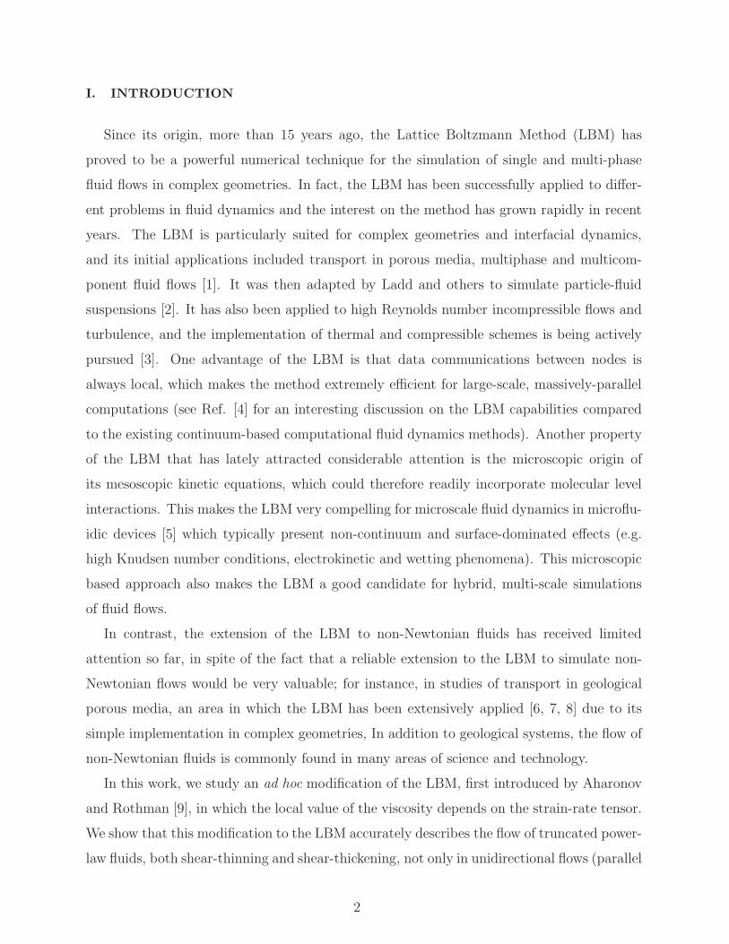
I. INTRODUCTION
Since its origin, more than 15 years ago, the Lattice Boltzmann Method (LBM) has
proved to be a powerful numerical technique for the simulation of single and multi-phase
fluid flows in complex geometries. In fact, the LBM has been successfully applied to differ-
ent problems in fluid dynamics and the interest on the method has grown rapidly in recent
years. The LBM is particularly suited for complex geometries and interfacial dynamics,
and its initial applications included transport in porous media, multiphase and multicom-
ponent fluid flows [1]. It was then adapted by Ladd and others to simulate particle-fluid
suspensions [2]. It has also been applied to high Reynolds number incompressible flows and
turbulence, and the implementation of thermal and compressible schemes is being actively
pursued [3]. One advantage of the LBM is that data communications between nodes is
always local, which makes the method extremely efficient for large-scale, massively-parallel
computations (see Ref. [4] for an interesting discussion on the LBM capabilities compared
to the existing continuum-based computational fluid dynamics methods). Another property
of the LBM that has lately attracted considerable attention is the microscopic origin of
its mesoscopic kinetic equations, which could therefore readily incorporate molecular level
interactions. This makes the LBM very compelling for microscale fluid dynamics in microflu-
idic devices [5] which typically present non-continuum and surface-dominated effects (e.g.
high Knudsen number conditions, electrokinetic and wetting phenomena). This microscopic
based approach also makes the LBM a good candidate for hybrid, multi-scale simulations
of fluid flows.
In contrast, the extension of the LBM to non-Newtonian fluids has received limited
attention so far, in spite of the fact that a reliable extension to the LBM to simulate non-
Newtonian flows would be very valuable; for instance, in studies of transport in geological
porous media, an area in which the LBM has been extensively applied [6, 7, 8] due to its
simple implementation in complex geometries, In addition to geological systems, the flow of
non-Newtonian fluids is commonly found in many areas of science and technology.
In this work, we study an ad hoc modification of the LBM, first introduced by Aharonov
and Rothman [9], in which the local value of the viscosity depends on the strain-rate tensor.
We show that this modification to the LBM accurately describes the flow of truncated power-
law fluids, both shear-thinning and shear-thickening, not only in unidirectional flows (parallel
2
Page 3
plates geometry) but also in two-dimensional flows with simultaneous shear components in
more than one direction (reentrant corner geometry).
II. LATTICE-BOLTZMANN METHOD
The LBM can be viewed as an implementation of the Boltzmann equation on a discrete
lattice and for a discrete set of velocity distribution functions [10],
fi(x+ ei∆x, t +∆t) = fi(x, t) + Ωi(f(x, t)), (1)
where fi is the particle velocity distribution function along the ith direction, Ωi(f(x, t)) is
the collision operator which takes into account the rate of change in the distribution function
due to collisions, ∆x and ∆t are the space and time steps discretization, respectively [1].
Then, the density ρ and momentum density ρu are given by the first two moments of the
distribution functions,
ρ =∑
i
fi, ρu =∑
i
fiei, (2)
where we assumed that the discretization is consistent with the Boltzmann equation, x+ ei
corresponding to the nearest neighbors of the point x. Note that in the previous equation,
and in the reminder of the article, all quantities are rendered dimensionless using ∆x and ∆t
as the characteristic space and time scales, respectively. Also note that, as we are concerned
with incompressible flows, we do not need to introduce a dimension of mass.
A. BGK Approximation
Assuming that the system is close to equilibrium the collision operator is typically lin-
earized about a local equilibrium distribution function, f eqi , and assuming further that the
local particle distribution relaxes to equilibrium with a single characteristic (relaxation) time
τ , we arrive at the Bhatnagar, Gross and Krook (BGK) approximation of the LBM [1],
fi(x + ei∆x, t +∆t) = fi(x, t) +fi(x, t)− f eq
i (x, t)
τ, (3)
where the relaxation time τ is directly related to the kinematic viscosity of the fluid, ν =
(2τ − 1)/6.
3
Page 4
B. Non-Newtonian flows
The ad hoc extension of the LBM proposed by Aharonov and Rothman [9] to simulate
non-Newtonian fluids consists of determining the value of the relaxation time τ locally,
in such a way that the desired local value of the viscosity is recovered. The viscosity is
related to the local rate-of-strain through the constitutive equation for the stress tensor. A
commonly used model of non-Newtonian fluids is the generalized Newtonian model, in which
the relation between the stress tensor, σij , and the rate-of-strain tensor, Dij , is similar to
that for Newtonian fluids, σij = 2µDij, but with µ a function of the invariants of the local
rate-of-strain tensor, µ = µ(Dij). In particular, we are interested in a widely used model:
the power-law expression [11], µ = mγn−1, where n > 0 is a constant characterizing the
fluid. The case n < 1 correspond to shear-thinning (pseudoplastic) fluids, whereas n > 1
correspond to shear-thickening (dilatant) fluids, and n = 1 recovers the Newtonian behavior.
The magnitude of the local shear-rate γ is related to the second invariant of the rate-of-strain
tensor, γ =√
DijDij , where the components of the rate-of-strain tensor, Dij , are computed
locally from the velocity field. In particular, after obtaining the instantaneous velocity field
from the LBM we then compute Dij from a first-order finite-difference approximation to the
local derivatives of the velocity.
However, there is an obvious obstacle to a direct implementation of the power-law fluid
in the LBM, in that the effective viscosity diverges for zero shear rates (γ = 0) in a shear-
thinning fluid ( n < 1). Analogously, the viscosity becomes zero for a shear-thickening fluid
at zero shear rates. In previous studies it is not clear how this problem was avoided.
Clearly, both limits are unphysical and, in fact, it is known that many non-Newtonian
fluids exhibit a power-law behavior only in some range of shear-rates, and a constant viscosity
is observed outside that range [11]. Here, we used the simplest model of such fluids: the
truncated power-law model,
ν(γ) = µ(γ)/ρ =
mγ(n−1)0 γ < γ0
mγ(n−1) γ0 < γ < γ∞
mγ(n−1)∞ γ > γ∞
(4)
Using the truncated power-law model has an additional advantage in the LBM. It is
well known that the LBM can accurately simulate viscous flows only in a limited range of
kinematic viscosities. The method becomes unstable for relaxation times close to τ >∼ 1/2
4
Page 5
[12] (small kinematic viscosities, ν <∼ 0.001) and its accuracy is very poor for τ >
∼ 1 [13]
(relatively large kinematic viscosities, ν >∼ 1/6). Therefore, we set the lower and upper
saturation values of the kinematic viscosity in Eq. (4) to νmin = 0.001 and νmax = 0.1. It is
clear that the maximum value of the viscosity corresponds to the value at zero shear rate
for shear-thinning fluids (n < 1), whereas the opposite is true for shear-thickening materials
(n > 1). Note that setting the value of the maximum model viscosity to νmax = 0.1
for a given maximum fluid viscosity ν⋆max and a spatial resolution ∆x simply corresponds
to choosing a particular value of the time step in order to satisfy, ν⋆max = νmax(∆x2/∆t)
[4]. Since the kinematic viscosity scales with ∆x2/∆t, to keep the dimensionless viscosity
constant we shall rescale ∆t according to the previous relationship when we increase the
number of lattice nodes N , that is, since ∆x ∝ 1/N then ∆t ∝ 1/N2. In what follow we use
the three-dimensional (face-centered-hypercubic) FCHC-projection model of the LBM with
19 velocities (D3Q19 following the notation in Ref. [14]).
III. FLOW BETWEEN PARALLEL PLATES
We first test the proposed LBM for non-Newtonian flows in a simple unidirectional flow,
the flow between two parallel plates separated a distance b in the z-direction (Hele-Shaw
cell) in the presence of a pressure gradient in the x-direction. We use periodic boundary
conditions in both x and y directions. The resulting flow field is unidirectional, with vx(z)
the only non-zero velocity component, the rate-of-strain is a scalar function of the local
velocity, γ = |dvx/dz|, and the Navier-Stokes equations are greatly simplified [15].
In order to compute the exact solution to the Navier-Stokes equations for a pressure driven
flow of a truncated power-law fluid in the Hele-Shaw geometry we split the system into (in
principle) three different regions. We shall describe the regions between z = 0 and z = b/2
and the analogous regions for z > b/2 follow by symmetry. The first region we consider is
the high-shear rate region close to the walls, Region H for z < zh, in which the shear rate
exceeds γ∞, and the fluid is Newtonian with effective kinematic viscosity ν∞ = mγ(n−1)∞ ; the
second one is the intermediate region in which the fluid behaves as a power law according
to Eq. (4), Region I for zh < z < zl; and the last one is the low-shear rate region close to the
center of the channel, Region L for zl < z < b/2, in which the shear rate is lower than γ0
and the fluid is again Newtonian, but with kinematic viscosity ν0 = mγ(n−1)0 . Matching then
5
Page 6
0 1 2 3 4 5 6 7 8 9 10z
0
2×10⁻⁴
4×10⁻⁴
6×10⁻⁴
8×10⁻⁴
1×10⁻³
u x
zlzl~
Parabolic profile
Power Law profile
Region L Region IRegion I
FIG. 1: Comparison between a Lattice-Boltzmann simulation and the analytical solution for the
flow between two parallel plates separated a distance b = 10. The power-law exponent of the fluid
is n = 0.50 (shear-thinning). The pressure gradient is ∇P = 6×10⁻⁶, ρ = 1, ν0 = 0.1, ν∞ = 0.001,
m = 10−3, and N = 400. The circles correspond to the Lattice-Boltzmann simulations. The
solid line corresponds to the analytical solution given by Eq. (5). Also shown, in dashed lines, are
the continuation of the Newtonian and Power-Law solutions outside their regions of applicability.
The vertical, dashed lines correspond to the transition points, zl and zl = b− zl, between the low
shear-rate region L, and the region of intermediate shear rates, I.
the solution obtained in each region with the conditions of continuity in the velocity and
the stress, we obtain the general solution to the problem, in terms of the pressure gradient
Gρ = −∇P ,
vx(z) =
(
G2ν∞
)
z(b − z) 0 ≤ z ≤ zh
nn+1
(
Gm
)1
n
[
(
b2
)n+1
n −(
b2− z
)n+1
n
]
+ α1 zh ≤ z ≤ zl(
G2ν0
)
z(b− z) + α2 zl ≤ z ≤ b/2
, (5)
6
Page 7
with the constants α1 and α2 given by,
α1 =
(
G
2ν∞
)
zh(b− zh)−n
n+ 1
(
G
m
)1
n
[
(
b
2
)n+1
n
−
(
b
2− zh
)n+1
n
]
, (6)
α2 =n
n+ 1
(
G
m
)1
n
[
(
b
2
)n+1
n
−
(
b
2− zl
)n+1
n
]
−
(
G
2ν0
)
zl(b− zl) + α1,
and the transition points, zh and zl,
zh =b
2−
( ν∞m1/n
)n
n−1 1
G=
b
2−
mγn∞
G, (7)
zl =b
2−
( ν0m1/n
)n
n−1 1
G=
b
2−
mγn0
G.
Clearly, the number of regions that coexist will depend on the magnitude of the imposed
pressure gradient G. For very small pressure gradients, G ≪ 1, both zh and zl become
negative (see the previous equation), which means that shear rates are smaller than γ0
across the entire gap and only Region L exists. As G increases, there is a range of pressure
gradients, mγn0 < (b/2)G < mγn
∞, for which zl > 0 but zh < 0, and therefore regions L and
I coexist. Finally, for G > (2/b)mγn∞ we obtain zh > 0, and all three regions are present in
the flow. Note that for large values of G both transition points converge to the center of the
cell, zl, zh → b/2. Thus, Eq. (7) allows us to choose the appropriate value of G in order to
investigate the different regimes.
We performed a large number of simulations for different values of the power-law exponent
n. Specifically, we consider two shear-thinning fluids, n = 0.50 and n = 0.75, and two shear-
thickening fluids, n = 1.25 and n = 2.00. In all cases we performed simulations for two
different magnitudes of the external forcing: one for which the region of low shear rates L is
important, that is relatively small pressure gradients for which zl ∼ b/4; and a second one
in which the fluid behaves as a power-law fluid almost in the entire gap, that is zl ∼ b/2. In
both cases the shear-rate does not exceeds γ∞. In Fig. 1 we present a comparison between the
Lattice-Boltzmann results and the analytical solution given in Eq. (5) for a shear-thinning
fluid with power-law exponent n = 0.50. The simulation corresponds to a relatively small
pressure gradient for which the region of small shear-rates is large, zl ∼ b/4. Both regions,
Region L in which the fluid behaves as a Newtonian one, and Region I in which the effective
viscosity is a power-law, are shown. The agreement with the analytical solution is excellent,
with relative error close to 0.1%. In Fig. 2 we present a similar comparison between the
7
Page 8
0 1 2 3 4 5 6 7 8 9 10z
0.0
4.0×10⁻³
8.0×10⁻³
1.2×10⁻²
1.6×10⁻²
2.0×10⁻²
u x
zl zl
Region IRegion I Reg
ion
L
~
FIG. 2: Comparison between a Lattice-Boltzmann simulation and the analytical solution for the
flow between two parallel plates separated a distance b = 10. The power-law exponent of the
fluid is n = 2.00 (shear-thickening). The pressure gradient is ∇P = 5 × 10⁻⁶, ρ = 1, ν0 = 0.001,
ν∞ = 0.1, m = 10−3, and N = 400. The circles correspond to the Lattice-Boltzmann simulations
and the solid line corresponds to the analytical solution given by Eq. (5). The vertical dashed lines
correspond to the transition points, zl and zl = b − zl, between the low shear-rate region L and
the intermediate shear rates region I.
LBM and the analytical solution, but for a shear-thickening fluid (n = 2.00) which behaves
as a power-law fluid across almost the entire channel. Again the agreement is excellent with
relative error smaller than 0.1%.
Finally, for each of these cases we run a series of simulations in which the number of
lattice nodes, N , in the direction of the gap was increased from 10 to 400, and computed the
relative error of the LBM results compared to the analytical solutions, defined as∑N
i=1(1−
vLBMi /vAnal.
i )2. In order to obtain the accuracy of the LBM as a function of the number of
nodes, we simulated the same physical problem but changed ∆x from 1 to 0.025. In addition,
8
Page 9
10 100Number of lattice nodes
10-3
10-2
10-1
Rel
ativ
e E
rror
n=0.50 Power Lawn=0.50 Intermediaten=0.75 Power Lawn=0.75 Intermediaten=1.25 Power Lawn=1.25 Intermediaten=2.00 Power Lawn=2.00 Intermediate
1/N
0.1% Error
FIG. 3: Relative error of the LBM compared to the analytical solution for the flow between parallel
plates, as a function of the number of lattice points used in the simulations. The points correspond
to simulations with the LBM for four different fluids, two shear-thinning fluids (n = 0.50 and
n = 0.75) and two shear-thickening fluids (n = 1.25 and n = 2.00). For all fluids we also present
results corresponding to two different regimes: one at high pressure gradients, in which the low-
shear-rates region, region L, is small (Power-Law) and the other one at intermediate pressure
gradients in which both regions L and I are comparable (note that with the exception of n = 0.75
both regimes give almost exactly the same relative error and, in fact, the corresponding points
overlap almost entirely). In all cases, we increased the lattice resolution until the relative error was
on the order of 0.1%. The solid line shows the general trend of the data, 1/N .
since the accuracy of the LBM depends on the model viscosity, we also changed ∆t according
to ∆t = ∆x2, so that the model viscosity remains the same, independent of the number of
nodes. Then, in order to compare the velocity field always at the same physical time since
startup, the number of time steps was increased inversely proportional to ∆t (reaching ∼ 108
9
Page 10
time steps for N = 400). In Fig. 3 we present the results obtained for the different fluids
and different pressure gradients. It is clear that, in all cases, the relative error decreases,
approximately as 1/N , as the number of nodes is increased, and eventually becomes of the
order of 0.1% (an arbitrary target accuracy that we set for our simulations). The error was
found to be independent of the pressure gradient, or the size of the non-Newtonian region
I, but strongly depends on the power-law exponent. In particular, the relative error seems
to increase as the magnitude of (1 − n)/n increases, with the error in the Newtonian case
(n = 1) decaying faster than 1/N . This is probably related to the first-order finite-difference
approximation used to compute the spatial derivatives of the fluid velocity which determine
the local viscosity through Eq. (4). It would then be possible to improve the accuracy of
the method by implementing a higher order approximation of the local shear-rates.
IV. REENTRANT CORNER FLOW
In the previous section we tested the LBM for non-Newtonian fluids in a Hele-Shaw
geometry and found excellent agreement with the analytical solutions as the number of
nodes was increased. In that case, the flow is unidirectional and therefore the shear-rate is
a scalar, which is a rather simple type of flow. In contrast, we shall now test the LBM in a
more demanding geometry, that is the reentrant corner geometry sketched in Fig. 4. In this
case, the shear-rate is no longer a scalar as in the Hele-Shaw geometry and, in addition, the
presence of two singular points, located at the entrant and reentrant corners (see Fig. 4),
requires high accuracy in order to obtain satisfactory stress resolution near these points
(although no analog to the Moffatt’s analysis near the corner is available for non-Newtonian
fluids, it is believed that not-integrable stress singularities develop in this case, and numerical
techniques do not always converge [16]). Motivated by these issues we simulated the flow
in the reentrant corner geometry using the LBM for a shear-thinning fluid with power-law
exponent n = 0.50. In Fig. 4 we present the streamlines corresponding to the computed
velocity field, obtained for a pressure gradient ∇P = 10−5, where the recirculation region
inside the cavity can be observed (note that the separation between streamlines was chosen
for visualization purposes only and it is not related to the local flow rate, since the magnitude
of the fluid velocity sharply decays inside the cavity). The corresponding Reynolds number
is Re = 4, computed with the maximum viscosity, ν0, and the measured mean velocity. In
10
Page 11
0 5 10 15 20 25 30 35 400
5
10
15
20
25
30
35
40
CornerReentrant
Corner
LineY=16
x
yLine
Entrant
X=20
FIG. 4: Streamlines in the reentrant flow geometry. The flow direction is shown at the center
of the channel. Note the asymmetry due to inertia effects. The dashed lines show the lines in
which we compare the solutions of the LBM method with the solutions obtained by finite-element
calculations.
fact, the streamlines shown in Fig. 4 are fore-aft asymmetric, due to inertia effects, which
are absent in low-Reynolds-number flows. We also computed the local magnitude of the
shear-rate, related to the local stress field through the constitutive relation given by Eq. (4).
In Fig. 5 we present a contour plot of the magnitude of the shear-rate in the reentrant
corner geometry with the lowest level in the contour plot corresponding to γ0. It can be
seen that the fluid is Newtonian in small regions at the center of the channel and inside the
recirculation region. It is also clear that, as discussed before, both the entrant and reentrant
corners are singular points where the shear-rate increases to its highest values in the system.
Finally, in order to perform a more quantitative test of the LBM, we solved the problem
11
Page 12
x
y
0 5 10 15 20 25 30 35 400
5
10
15
20
25
30
35
40
1
2
3
4
5
6
7
8
9
x 10−3
.
ReentrantCorner
γ
Entrant
0
Corner
FIG. 5: Contour-plot of the local magnitude of the shear-rate, as computed with the LBM. The
lowest level of the plot corresponds to γ0, that is the fluid behaves as Newtonian in those regions.
High shear-rates, and accordingly high shear-stresses are localized at the entrant and reentrant
corners.
numerically using the finite-element commercial software FIDAP (Fluent Inc.). In Figs. 6
and 7 we compare the solutions obtained with the LBM for different resolutions, ranging
from N = 40 × 40 to N = 320× 320, with the finite-element results obtained with FIDAP.
The comparison is made along two lines, one oriented along the flow direction (dashed line
at Y = 16 in Fig. 4) and a second one oriented in the perpendicular direction (dashed line
at X = 20 in Fig. 4). In Fig. 6 we compare the velocity along the channel, ux, in the line
perpendicular to x that is located at the center of the system (X = 20, see Fig. 4). A
velocity profile similar to that in a Hele-Shaw cell is observed for 0 < y <∼ 20, as well as
the recirculation flow inside the cavity (see the inset). In Fig. 7 we plot the velocity in the
12
Page 13
0 10 20 30 40z
0.0
1.0×10⁻²
2.0×10⁻²
3.0×10⁻²
u x
Finite-Element SolutionN = 320 x 320N = 80 x 80N = 40 x 40
20 30 40
z
0.0
1.0×10⁻³
u x
FIG. 6: Velocity component along the channel, ux, plotted in a line perpendicular to the flow
(dashed line X = 20 in Fig. 4). We compare the results of the finite-element calculations (solid
line) with the results of the LBM (points) for different lattice resolutions. In the inset we plot the
velocity profile inside the recirculation region.
vertical direction, uy, along a horizontal line close to the upper wall of the channel (Y = 16,
see Fig. 4). It is clear that there is some fluid penetration into the cavity (entrant flow)
in the first half of the channel and some reentrant flow in the second half (note that, as
mentioned before, the flow is not symmetric about x = 20 due to inertia effects). In both
cases we found an excellent agreement between the two methods, and the agreement clearly
improved as the number of lattice nodes was increased in the LBM (the number of elements
in the finite-element computations was fixed to 100× 100).
13
Page 14
0 10 20 30 40
x-3×10⁻³
-2×10⁻³
-1×10⁻³
0
1×10⁻³
2×10⁻³
3×10⁻³
u y
Finite-Element SolutionN = 320 x 320N = 80 x 80N = 40 x 40
FIG. 7: Velocity component perpendicular to the flow direction, uy, plotted in a line parallel to
the flow and close to the top wall of the channel (dashed line Y = 16 in Fig. 4). We compare
the results of the finite-element calculations (solid line) with the results of the LBM (points) for
different lattice resolutions.
V. CONCLUSIONS
We have extensively tested an ad hoc modification of the Lattice-Boltzmann Method
that extends its use to Generalized Newtonian fluids, in which the non-Newtonian character
of the fluids is modelled as an effective viscosity. Specifically, we calculated the accuracy
of the method for Truncated Power-Law fluids and showed that the relative error decays
(linearly) as the resolution of the lattice (number of lattice points) is increased. The error
was computed directly from the analytical solutions of the problem. The same trend was
observed for both shear-thinning (n < 1) and shear-thickening (n > 1) fluids, as well as for
intermediate and high shear-rates. In all cases the relative error was of the order of 0.1% for
the highest resolution employed. Finally, we also tested the method in the reentrant flow
geometry and showed that it is in excellent agreement with the solution obtained by means
14
Page 15
of finite-element calculations. Again, the accuracy of the method was shown to increase
with the number of lattice points.
Acknowledgments
This work is part of a collaboration supported by the Office of International Science and
Engineering of the National Science Foundation under Grant No. INT-0304781. This re-
search was supported by the Geosciences Research Program, Office of Basic Energy Sciences,
U.S. Department of Energy, and computational facilities were provided by the National En-
ergy Resources Scientific Computer Center.
[1] S. Chen and G. D. Doolen, Ann. Rev. Fluid Mech. 30, 329 (1998).
[2] A. J. C. Ladd and R. Verberg, J. Stat. Phys. 104, 1191 (2001).
[3] D. Z. Yu, R. W. Mei, L. S. Luo, and S. Wei, Prog. Aerosp. Sci. 39, 329 (2003).
[4] R. R. Nourgaliev, T. N. Dinh, T. G. Theofanous, and D. Joseph, Int. J. Mult. Flow 29, 117
(2003).
[5] D. Raabe, Modelling Simul. Mater. Sci. Eng. 12, R13 (2004).
[6] G. Drazer and J. Koplik, Phys. Rev. E 62, 8076 (2000).
[7] G. Drazer and J. Koplik, Phys. Rev. E 63, 056104 (2001).
[8] G. Drazer and J. Koplik, Phys. Rev. E 66, 026303 (2002).
[9] E. Aharonov and D. H. Rothman, Geophys. Res. Lett. 20, 679 (1993).
[10] D. H. Rothman and S. Zaleski, Lattice-Gas Cellular Automata, Simple Models of Complex
Hydrodynamics (Cambridge University Press, Cambridge, UK, 1997).
[11] R. B. Bird, W. E. Stewart, and E. N. Lightfoot, Transport Phenomena (Wiley Text Books,
New York, 2001), 2nd ed.
[12] X. D. Niu, C. Shu, Y. T. Chew, and T. G. Wang, J. Stat. Phys. 117, 665 (2004).
[13] O. Behrend, R. Harris, and P. B. Warren, Phys. Rev. E 50, 4586 (1994).
[14] Y. H. Qian, D. D’Humieres, and P. Lallemand, Europhys. Lett. 17, 479 (1992).
[15] L. G. Leal, Laminar Flow and Convective Transport Processes (Butterworth-Heinemann,
1992).
15
Page 16
[16] J. Koplik and J. R. Banavar, J. Rheol. 41, 787 (1997).
16