Lattice Theory Lecture 4

Non-distributive lattices

John Harding

New Mexico State Universitywww.math.nmsu.edu/∼JohnHarding.html

jharding@nmsu.edu

Toulouse, July 2017

Introduction

Here we mostly consider modular lattices, but also make somecomments on free lattices.

Understanding free lattices is key to many aspects of lattice theoryincluding projectives.

We won’t have time for these other aspects, but will describe thefree lattice FL(X ) on a set X and show that the class Lat of alllattices has decidable equational theory.

2 / 44

Free Lattices

As with free distributive lattices and free Boolean algebras, the freelattice FL(X ) is given by equivalence classes of terms T (X )/ ≡.Here equivalence

(x ∧ y) ∧ (x ∨ x) ≡ x ∧ y

means that the terms evaluate to the same in every lattice.

Unlike the distributive and Boolean case there is no test simplealgebra such as 2, so no analog of the method of truth tables. Weneed a different way to describe ≡.

3 / 44

Free Lattices

Definition Let ⊑ be the smallest relation on the set of lattice termsT (X ) using variables from X such that

1. x ⊑ x for each x ∈ X2. if p ⊑ s then p ∧ q ⊑ s

3. if q ⊑ s then p ∧ q ⊑ s

4. if p ⊑ s then p ⊑ s ∨ t

5. if p ⊑ t then p ⊑ s ∨ t

These are called Whitman’s conditions.

Note, one can construct ⊑ recursively on the complexity of terms,so can effectively tell whether p ⊑ q.

4 / 44

Free Lattices

Proposition The relation ⊑ is reflexive and transitive, hence is aquasi-order on T (X ).

Pf A bit of an onerous inductive proof. Try it!

From Lecture 1, a quasi-order ⊑ on a set P has an associatedequivalence relation θ on P given by p θq iff p ⊑ q and q ⊑ p, andthen a partial order ≤ on P/θ given by p/θ ≤ q/θ iff p ⊑ q.

Definition Let θ and ≤ be the equivalence relation and partialordering for T (X ) given by ⊑.

5 / 44

Free Lattices

Theorem (Whitman) Lattice terms s, t evaluate to the same inevery lattice iff sθt in the relation θ given by the quasi-order ⊑.

Pf “⇐” The conditions for ⊑ are very sparse, so if s ⊑ t then inany lattice L we have sL ≤ tL.

“⇒” We need that if s /θ t then sL ≠ tL in some lattice L. To dothis we show that T (X )/θ is a lattice! This is an even nastierinductive proof to show that if p,q ⊑ s, then p ∨ q ⊑ s.

Corollary The free lattice on a set X is T (X )/θ

6 / 44

Free Lattices

Remarks

• The free lattice on 2 generators is a 4-element lattice.

• The free lattice on 3 generators is infinite

• The free lattice on 3 generators contains a sublatticeisomorphic to the free lattice on countably many generators.

• The free lattice FL(X ) has no uncountable chains

Exercise Is N5 a sublattice of FL(3)? Much harder — is M5?

7 / 44

Modular Lattices

Here we try to explain why people would be interested in modularlattices.

We begin with an example, but first need a definition.

Definition An element c in a complete lattice L is compact ifwhenever c ≤ ⋁S then c ≤ ⋁S ′ for some finite S ′ ⊆ S . L isalgebraic if each element is the join of compact ones.

Proposition A closure system C forms an algebraic lattice if it isalso closed under unions of non-empty chains.

8 / 44

Vector Spaces

Definition For V a vector space over a field F , let S(V ) be thecollection of subspaces of V partially ordered by set inclusion.

Proposition For a vector space V , the poset S(V ) is

1. a complete lattice

2. atomistic

3. algebraic

4. complemented

5. directly irreducible

6. modular

Call a lattice with these properties geomodular.

9 / 44

Vector Spaces

Pf 1. The intersection of subspaces is a subspace. So S(V ) is acomplete lattice where meets are intersections. The join of twosubspaces is

S ∨T = {s + t ∶ s ∈ S , t ∈ T}

2. The atoms are 1-dimensional subspaces. Each subspace is theunion of these, hence its atomistic.

3. Algebraic since closed under unions of chains.

4. Complemented: Given a subspace S find a basis X of S .Extend this to a basis X ∪Y of V . Then for T = span Y we haveS ∩T = {0} and S ∨T = V . So T is a complement of S .

10 / 44

Vector Spaces

5. If S(V ) ≃ L1 × L2 then there would be an element (1,0) in itthat is not a bound and has exactly one complement. A subspaceS that is not a bound always has more than one complement sinceits basis X can be extended to a basis of V in many ways.

6. Let S ,T ,U be subspaces with S ⊆ U. We need

S ∨ (T ∩U) = (S ∨T ) ∩U

That ⊆ holds is trivial. For ⊇ suppose x ∈ RHS. Then x ∈ U andx = s + t for some s ∈ S , t ∈ T . Then t = x − s and since x , s ∈ U wehave t ∈ U. So x = s + t where s ∈ S , t ∈ T ∩U gives x ∈ LHS.

11 / 44

Vector spaces

Example Lets consider subspaces of R, R2, R3.

S(R) S(R2) S(R3)

lines

planes

Both S(R2) and S(R3) are infinite, we show only part.

S(R2) ∶ {0}, lines through the origin, R2

S(R3) ∶ {0}, lines through the origin, planes through the origin, R3

12 / 44

Dimension

Subspaces of a vector space and modular lattices share several keyproperties. Finite-dimensional vector spaces have a dimensionfunction. There is an analog for modular lattices of finite height.

Proposition Let M be a modular lattice where every chain is finite.Then for each x ∈M every maximal chain in [0, x] has the samenumber of elements. We define h ∶M → N by

h(x) = the length of a maximal chain in [0, x] − 1

Proposition In the appropriate setting

1. dim S + dim T = dim (S ∨T )− dim (S ∧T )2. h(x) + h(y) = h(x ∨ y) − h(x ∧ y)

13 / 44

Links to Geometry

Suppose we have a 3-dimensional vector space V . If we think ofthe 1-dimensional subspaces as points of a geometry, and the2-dimensional subspaces as lines of a geometry, we have

• any two points lie on a unique line

• any two lines intersect in a unique point

The second item is because

dim (S ∧T ) = dim S + dim T − dim (S ∨T ) = 2 + 2 − 3

This is the idea behind a projective plane. The exact definition of aprojective geometry will account for higher dimensions as well.

14 / 44

Projective Geometry

Example Consider the subspaces of (Z2)3, a three-dimensionalvector space over the 2-element field. We draw 1-dimensionalsubspaces as points, and 2-dimensional ones as lines.

Fano plane

Exercise If the corners of the triangle are the 1-dimensionalsubspaces ⟨(1,0,0)⟩, ⟨(0,1,0)⟩, ⟨(0,0,1)⟩ label the rest. Hint, themiddle is ⟨(1,1,1)⟩ and the line at bottom is the plane y = 0.

15 / 44

Projective Geometry

Definition A projective geometry G = (P,L, I) consists of a set P ofpoints, a set L of lines, and a relation I ⊆ P ×L where

1. any two distinct points lie on a unique line

2. pq′r , p′qr collinear ⇒ exists r ′ with pqr ′, p′q′r ′ collinear

Item 2 says that coplanar lines intersect.

Definition If G is a projective geometry, then a subset S ⊆ P is asubspace of G if p,q ∈ S and pqr collinear ⇒ r ∈ S .

16 / 44

The Connections

Proposition Let V be a vector space over a division ring D. Set

1. P = the one-dimensional subspaces of V

2. L = the two-dimensional subspaces of V

3. p IL ⇔ p is contained in L

Then G = (P,L, I) is a projective geometry.

Pf Two points (1-dim subspaces) span a line (2-dim subspace).Let S ,T be lines (2-dim subspaces). Having them coplanar meansdim (S ∨T ) = 3. Then

dim (S ∩T ) = dim S + dim T− dim (S ∨T ) = 2 + 2 − 3 = 1

So coplanar lines meet in a point.

17 / 44

The Connections

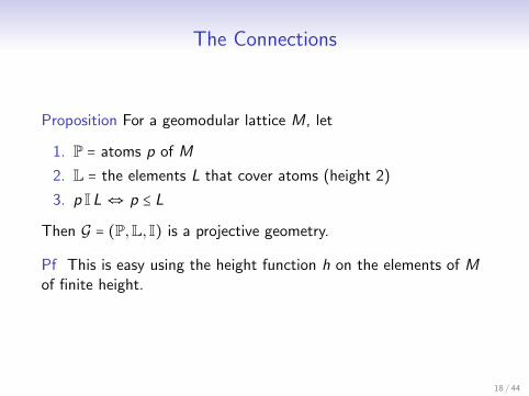
Proposition For a geomodular lattice M, let

1. P = atoms p of M

2. L = the elements L that cover atoms (height 2)

3. p IL ⇔ p ≤ L

Then G = (P,L, I) is a projective geometry.

Pf This is easy using the height function h on the elements of Mof finite height.

18 / 44

The Connections

Proposition For a projective geometry G, its subspaces S(G),partially ordered by set inclusion form a geomodular lattice.

Pf The intersection of subspaces is a subspace and the union of achain of subspaces is a subspace. This shows it is complete andalgebraic. The atoms are the singletons {p} for a point p, so it isatomistic. The other items require a description of the join of twosubspaces S ,T when neither contains the other and are similar tothe proofs for S(V ).

S ∨T = {r ∶ there are s ∈ S and t ∈ T with rst collinear}

Exercise complete the proof.

19 / 44

The Connections

So far we have shown the following relationships.

VectorSpaces

ProjectiveGeometries

GeomodularLattices

20 / 44

The Connections

Completing the equivalences doesn’t quite work. We require anadditional geometric condition on the projective geometry knownas Desargue’s law (1600’s!). Its correspondent for geomodularlattices becomes an equation known as the Arguesian equation.

Assuming this, we can construct from a Desarguesian projectivegeometry G a division ring D and vector space V over D with Gthe projective geometry built from V .

The ideas are 1000’s of years old. We briefly describe them.

21 / 44

Constructing a Vector Space from G

Step 1 Choose two distinct points O and E and let D be thepoints on the line OE .

O E

Eventually D will be the division ring and O,E will be its 0,1.

22 / 44

There are no parallel lines in a projective plane, but if we pick adistinguished line and call it the “line at infinity L∞”, then we calllines parallel if their intersection is on L∞.

Step 2 We add points A,B as follows.

O A B A +BO

O ′

23 / 44

Step 3 We multiply points as follows.

O EB A

E ′

AB

There is a lot to show that this all works, but it does if we haveDesargue’s law. Multiplication being commutative is equivalent toPappus’ law, another geometric condition.

24 / 44

The Connections

We wind up with nearly an object level equivalence. If you want tolook further at moving towards a full categorical treatment, see thebook by Faure and Frolicher.

VectorSpaces

ProjectiveGeometries

GeomodularLattices

25 / 44

Modular Lattices

Modular lattices play important roles in algebra, geometry, andcombinatorics. It would be good to have a nice theory of them aswith distributive lattices. But there are problems.

Theorem The free modular lattice on 3 generators has 28 elements,the free one on 4 or more generators is infinite.

Theorem The equational theory of modular lattices is undecidable.

Lets see how a 4-generated modular lattice can be infinite. It goesa long way to making the connection between vector spaces,modular lattices, and geometry concrete.

26 / 44

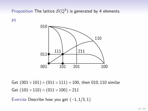
Proposition The lattice S(Q3) is generated by 4 elements.

Pf

001 101 201 100

011

010

111 211

110

Get (001 ∨ 101) ∧ (011 ∨ 111) = 100, then 010,110 similar

Get (101 ∨ 110) ∧ (011 ∨ 100) = 211

Exercise Describe how you get (−1,1/3,1)

27 / 44

Past Modular Lattices

In a somewhat mysterious way, modularity + complementation ismuch stronger than just modularity.

Theorem (Frink) Every complemented modular lattice M can beembedded into a possibly reducible geomodular one.

Pf Difficult. One constructs a geometry from the filters of M.

Corollary There is a modular lattice that cannot be embedded intoa complemented modular lattice.

Pf Take a non-Desarguesian irreducible modular lattice withheight > 3. Every geomodular lattice of height > 3 is Desarguesian.

28 / 44

Past Modular Lattices

Exercise Show that every lattice can be embedded into acomplemented lattice. Hint: if it is bounded, you only need toinclude one more element!

Exercise Show that every distributive lattice can be embedded intoa Boolean algebra. Hint: Use theorems we learned.

29 / 44

Past Modular Lattices

Subspace lattices S(V ) for a vector space V , are complemented.But often there is even more — a distinguished complement.

Definition An real inner product on a real vector space V is a map⟨ ⋅ , ⋅ ⟩ ∶ V 2 → R where

1. ⟨x , y⟩ = ⟨y , x⟩2. ⟨λx , y⟩ = λ ⟨x , t⟩3. ⟨x + y , z⟩ = ⟨x , z⟩ + ⟨y + z⟩4. ⟨x , x⟩ ≥ 0 with equality iff x = 0.

All we will say works for complex inner products as well, we usereal ones for simplicity here.

30 / 44

Past Modular Lattices

Example On Rn the familiar “dot product” is an inner productgiven by

(x1, . . . , xn) ⋅ (y1, . . . , yn) = x1y1 +⋯ + xnyn

Example On the vector space L2(X , µ) of a.e. classes of squareintegrable functions on a measure space (X , µ), there is an innerproduct given by

⟨ f , g ⟩ = ∫ f (x)g(x)dµ

This is an example of a Hilbert space, a primary ingredient inmodern physics and differential equations.

31 / 44

Past Modular Lattices

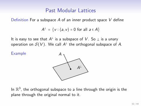
Definition For a subspace A of an inner product space V define

A⊥ = {v ∶ ⟨a, v⟩ = 0 for all a ∈ A}

It is easy to see that A⊥ is a subspace of V . So ⊥ is a unaryoperation on S(V ). We call A⊥ the orthogonal subspace of A.

Example A

A⊥

In R3, the orthogonal subspace to a line through the origin is theplane through the original normal to it.

32 / 44

Ortholattices

Definition An ortholattice is an algebra (L,∧,∨,0,1,⊥) where

1. (L,∧,∨,0,1) is a bounded lattice

2. x ∧ x⊥ = 0

3. x ∨ x⊥ = 1

4. x = x⊥⊥

5. x ≤ y ⇒ y⊥ ≤ x⊥

Example Every Boolean algebra is an ortholattice. In fact,Boolean algebras are exactly the distributive ortholattices.

33 / 44

Ortholattices

Proposition For any finite dimensional inner product space V , thelattice of subspaces (S(V ),⊥) is a modular ortholattice.

Pf Its easy to see A⊥ is a subspace and A ⊆ B ⇒ B⊥ ⊆ A⊥. Wealso have A ∩A⊥ = {0} since v in both gives ⟨v , v⟩ = 0, so v = 0.

The crucial point is that A ∨A⊥ = V . It follows from the fact thatany vector v is given by the sum of the projections

v = vA + vA⊥

That A⊥⊥ = A is then an exercise.

34 / 44

Ortholattices

For an infinite dimensional inner product space, it is not the casethat for each subspace A we have

v = vA + vA⊥

Indeed, we can’t even define the projection vA for arbitrary A.

A Hilbert space such as L2(X , µ) is a complete metric space underthe topology given by the norm and we can define the projectionvA when A is a closed subspace. It is the vector in A closest to v .

Key Lemma If A is a closed subspace of a Hilbert space H, thenA⊥ is a closed subspace and for each v we have v = vA + vA⊥ .

35 / 44

Ortholattices

Theorem Let H be a Hilbert space. Then its collection C(H) ofclosed subspaces has the following properties

1. it is complete as a lattice

2. it is an ortholattice

3. it satisfies A ⊆ B ⇒ A ∨ (A⊥ ∩B) = B

Note, C(H) is modular iff H is finite-dimensional. This is becausejoins are more complex, they are the closure of the span.

36 / 44

Orthomodular Lattices

Definition An ortholattice L is an orthomodular lattice if it satisfies

x ≤ y ⇒ x ∨ (x⊥ ∧ y) = y

Examples of orthomodular lattices include

• any Boolean algebra

• any modular ortholattice

• the closed subspaces C(H) Hilbert space

• the projections of a von Neumann algebra (from analysis)

Note modular + ortholattice ⇒ orthomodular lattice, not ⇐

37 / 44

Orthomodular Lattices

Example The following is an orthomodular lattice

0

1

a b c d e

a′ b′ c ′ d ′ e′

Note that the part at the left is an 8-element Boolean algebra, asis the part at right. Every orthomodular lattice is built by “gluingtogether” Boolean algebras in a sense we can make precise.

38 / 44

Orthomodular Lattices

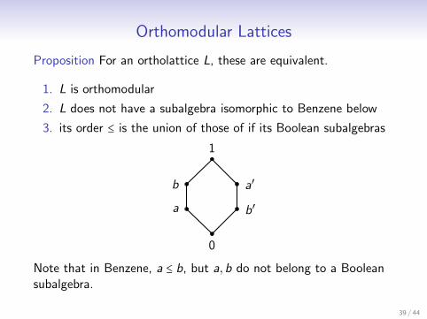
Proposition For an ortholattice L, these are equivalent.

1. L is orthomodular

2. L does not have a subalgebra isomorphic to Benzene below

3. its order ≤ is the union of those of if its Boolean subalgebras

0

1

a

b

b′

a′

Note that in Benzene, a ≤ b, but a,b do not belong to a Booleansubalgebra.

39 / 44

Orthomodular Lattices

Remark The study of orthomodular lattices has two parts. One isthe study of Boolean algebras and classical issues related to them.

The second is in how these Boolean algebras are “glued together”to form an orthomodular lattice. This second part contains thegeometric content that can be very challenging.

Example The subspaces S(R3) are built from 8-element Booleanalgebras ”glued together”. From the way they are glued, we canreconstruct R3. This gluing contains the full geometric content!

40 / 44

Orthomodular Lattices

For a Hilbert space H, the Boolean subalgebras of C(H) are key tospectral representations.

Spectral Theorem For a self-adjoint operator A on H there is aBoolean subalgebra B of C(H) and, for X = β(B) its Stone space,a representation of A by a continuous function f ∶ X → [−∞,∞].

X

−∞

∞

f

41 / 44

Orthomodular Lattices

This result was discovered in part by Marshall Stone, an analyst. Itwas the reason for his work on Boolean algebras and Stone spaces.

There is much more to all this.

Theorem (Takeuti) The self-adjoint operators affiliated with amaximal Boolean subalgebra B of C(H) correspond to the realnumbers in a B-valued model of set theory.

42 / 44

Final Comment

A growing trend is study of “quantum” or “non-commuative”versions of classical topics, such as non-commutative geometry.

Something to look for with these is the idea of versions of aclassical structure being “glued together” with the gluing providinggeometric content. Orthomodular lattices are a simple example,being a quantum, or non-commutative version of Boolean algebras.

Analogy

distributive lattices ∶∶ modular lattices

diagonal matrices ∶∶ matrices

43 / 44

Thanks for listening.

Papers at www.math.nmsu.edu/∼jharding