Laura Xiaolei Liutheinvestmentcapm.com/LiuWhitedZhang09JPE.pdfLaura Xiaolei Liu Hong Kong University...

1105

[ Journal of Political Economy, 2009, vol. 117, no. 6]� 2009 by The University of Chicago. All rights reserved. 0022-3808/2009/11706-0004$10.00

Investment-Based Expected Stock Returns

Laura Xiaolei LiuHong Kong University of Science and Technology

Toni M. WhitedUniversity of Rochester

Lu ZhangUniversity of Michigan and National Bureau of Economic Research

We derive and test q-theory implications for cross-sectional stock re-turns. Under constant returns to scale, stock returns equal leveredinvestment returns, which are tied directly to firm characteristics.When we use generalized method of moments to match average lev-ered investment returns to average observed stock returns, the modelcaptures the average stock returns of portfolios sorted by earningssurprises, book-to-market equity, and capital investment. When we tryto match expected returns and return variances simultaneously, thevariances predicted in the model are largely comparable to thoseobserved in the data. However, the resulting expected return errorsare large.

I. Introduction

We use the q-theory of investment to derive and test predictions for thecross section of stock returns. Under constant returns to scale, stock

We have benefited from helpful comments of Ilona Babenko, Nick Barberis, DavidBrown, V. V. Chari, Harry DeAngelo, Du Du, Wayne Ferson, Simon Gilchrist, Rick Green,Burton Hollifield, Liang Hu, Patrick Kehoe, Bob King, Narayana Kocherlakota, LeonidKogan, Owen Lamont, Sydney Ludvigson, Ellen McGrattan, Antonio Mello, Jianjun Miao,Mark Ready, Bryan Routledge, Martin Schneider, Jun Tu, Masako Ueda, Jiang Wang, and

1106 journal of political economy

returns equal levered investment returns. The latter returns are tied tofirm characteristics via firms’ first-order conditions for equity value max-imization. We use generalized method of moments (GMM) to matchmeans and variances of levered investment returns with those of stockreturns. We conduct the GMM tests using data on portfolios sorted byearnings surprises, book-to-market equity, and capital investment, whichare firm characteristics tied closely to cross-sectional patterns in returns.We also compare the performance of the q-theory model with the per-formance of traditional asset pricing models such as the capital assetpricing model (CAPM), the Fama-French (1993) three-factor model,and the standard consumption-CAPM with power utility.

When matching the average returns of the testing portfolios, the q-theory model outperforms the traditional models. We estimate a meanabsolute error of 0.7 percent per year for 10 equal-weighted portfoliossorted by earnings surprises. This error is lower than those from theCAPM, 5.7 percent, the Fama-French model, 4.0 percent, and the stan-dard consumption-CAPM, 3.6 percent. The error for the return on theportfolio that is long on stocks with high earnings surprises and shorton stocks with low earnings surprises (high-minus-low earnings surpriseportfolio) is �0.4 percent per year. This error is negligible comparedto the errors of 12.6 percent from the CAPM, 14.1 percent from theFama-French model, and 13.4 percent from the standard consumption-CAPM. Similarly, the q-theory model produces an error for the high-minus-low book-to-market portfolio of only 1.2 percent per year, whichis smaller than 18.6 percent from the CAPM, 7.3 percent from the Fama-French model, and 12.3 percent from the standard consumption-CAPM.Finally, the q-theory model produces an error for the high-minus-lowcapital investment portfolio of �0.5 percent per year, which is smallerthan the error of �6.3 percent from the CAPM, �6.3 percent from theFama-French model, and �8.4 percent from the standard consumption-CAPM.

other seminar participants at Boston University, Brigham Young University, Carnegie Mel-lon University, Emory University, Erasmus University Rotterdam, Federal Reserve Bank ofMinneapolis, Florida State University, Hong Kong University of Science and Technology,INSEAD, London Business School, London School of Economics, New York University,Purdue University, Renmin University of China, Shanghai Jiao Tong University, TilburgUniversity, University of Arizona, University of Lausanne, University of Southern California,University of Vienna, University of Wisconsin–Madison, Yale School of Management, So-ciety of Economic Dynamics annual meetings in 2006, University of British ColumbiaPhillips, Hager & North Centre for Financial Research Summer Finance Conference in2006, American Finance Association annual meetings in 2007, the China InternationalConference in Finance in 2007, and the Centre for Economic Policy Research Asset PricingWeek in Gerzensee in 2009. Liu acknowledges financial support from Hong Kong Uni-versity of Science and Technology (grant SBI07/08.BM04). We especially thank MonikaPiazzesi (the editor) and four anonymous referees for helpful comments. Online App. Dcontains unabridged tables and all the robustness tests not reported in the paper. Thispaper supersedes our NBER Working Paper no. 13024 titled “Regularities.”

investment-based expected stock returns 1107

When we use the q-theory model to match the average returns andvariances of the testing portfolios simultaneously, the variances pre-dicted by the model are largely comparable to stock return variances.The average stock return volatility across the earnings surprise portfoliosis 21.1 percent per year, which is close to the average levered investmentreturn volatility of 20.4 percent. The average realized and predictedvolatilities also are close for the book-to-market portfolios, 25.0 percentversus 23.6 percent, and for the capital investment portfolios, 24.8 per-cent versus 24.4 percent. However, the model falls short in two ways.First, while we find no discernible relation between volatilities and firmcharacteristics in the data, the model predicts a positive relation betweenvolatilities and book-to-market. Second, the resulting expected returnerrors vary systematically with earnings surprises and capital investmentand are comparable in magnitude to those from the traditional models.

Although q-theory originates in Brainard and Tobin (1968) and Tobin(1969), our work is built more directly on Cochrane (1991), which firstuses q-theory to study stock market returns, as well as on Cochrane(1996), which uses aggregate investment returns to parameterize thestochastic discount factor in cross-sectional tests. Several more recentarticles model cross-sectional returns based on firms’ dynamic optimi-zation problems (e.g., Berk, Green, and Naik 1999; Zhang 2005). Wediffer by doing structural estimation of closed-form Euler equations.Our work is also connected to the literature that estimates investmentEuler equations using aggregate or firm-level investment data (e.g., Sha-piro 1986; Whited 1992). Our work differs because we use this frame-work to study cross-sectional returns rather than investment dynamicsor financing constraints. Most important, our q-theory approach to un-derstanding cross-sectional returns represents a fundamental departurefrom the traditional consumption-based approach (e.g., Hansen andSingleton 1982; Lettau and Ludvigson 2001) in that we do not makeany preference assumptions.

II. The Model of the Firms

Time is discrete and the horizon infinite. Firms use capital and costlesslyadjustable inputs to produce a homogeneous output. Firms choose theselatter inputs each period, while taking their prices as given, to maximizeoperating profits. The operating profits are defined as revenues minusthe expenditures on these inputs. Taking operating profits as given,firms choose optimal investment and debt to maximize the market valueof equity.

Let denote the maximized operating profits of firm i atP(K , X )it it

time t. The profit function depends on capital, , and a vector ofKit

exogenous aggregate and firm-specific shocks, . We assume that firmXit


i has a Cobb-Douglas production function with constant returns toscale. The assumption of constant returns means that P(K , X ) pit it

. The Cobb-Douglas functional form means that theK �P(K , X )/�Kit it it it

marginal product of capital is given by , in�P(K , X )/�K p aY /Kit it it it it

which is capital’s share and is sales. This parameterization as-a 1 0 Yit

sumes that shocks to operating profits, , are reflected in sales.Xit

End-of-period capital equals investment plus beginning-of-period cap-ital net of depreciation: , in which capital de-K p I � (1 � d )Kit�1 it it it

preciates at an exogenous proportional rate of , which is firm specificdit

and time varying. Firms incur adjustment costs when investing. Theadjustment cost function, denoted , is increasing and convexF(I , K )it it

in , is decreasing in , and exhibits constant returns to scale inI K Iit it it

and : . We use a stan-K F(I , K ) p I �F(I , K )/�I � K �F(I , K )/�Kit it it it it it it it it it it

dard quadratic functional form: , in which2F(I , K ) p (a/2)(I /K ) Kit it it it it

.a 1 0Firms can finance investment with debt. We follow Hennessy and

Whited (2007) and model only one-period debt. At the beginning oftime t, firm i can issue an amount of debt, denoted , which mustBit�1

be repaid at the beginning of period . The gross corporate bondt � 1return on , denoted , can vary across firms and over time. TaxableBB rit it

corporate profits equal operating profits less capital depreciation, ad-justment costs, and interest expenses: P(K , X ) � d K � F(I , K ) �it it it it it it

, in which adjustment costs are expensed, consistent with treat-B(r � 1)Bit it

ing them as forgone operating profits. Let denote the corporate taxtt

rate at time t. The payout of firm i equals

BD { (1 � t)[P(K , X ) � F(I , K )] � I � B � r Bit t it it it it it it�1 it it

B� td K � t(r � 1)B , (1)t it it t it it

in which is the depreciation tax shield and is theBtd K t(r � 1)Bt it it t it it

interest tax shield.Let be the stochastic discount factor from t to , which isM t � 1t�1

correlated with the aggregate component of . Taking as ex-X Mit�1 t�1

ogenous, firm i maximizes its cum-dividend market value of equity:

�

V { max E M D , (2)�it t t�s it�s[ ]� sp0{I ,K ,B }it�s it�s�1 it�s�1 sp0

subject to a transversality condition that prevents firms from bor-rowing an infinite amount to distribute to shareholders:

.lim E [M B ] p 0Tr� t t�T it�T�1


Proposition 1. Firms’ equity value maximization implies that, in which is the investment return, defined asI IE [M r ] p 1 rt t�1 it�1 it�1

2Y a Iit�1 it�1Ir { (1 � t ) a � � t dit�1 t�1 t�1 it�1( ){ [ ]K 2 Kit�1 it�1

I Iit�1 it� (1 � d ) 1 � (1 � t )a 1 � (1 � t)a . (3)Zit�1 t�1 t( ) ( )[ ]} [ ]K Kit�1 it

Define the after-tax corporate bond return as Ba B Br { r � (r �it�1 it�1 it�1

; then . Define as the ex-dividendBa1)t E [M r ] p 1 P { V � Dt�1 t t�1 it�1 it it it

equity value, as the stock return, andSr { (P � D )/P w {it�1 it�1 it�1 it it

as the market leverage; then the investment return isB /(P � B )it�1 it it�1

the weighted average of the stock return and the after-tax corporatebond return:

I Ba Sr p w r � (1 � w )r . (4)it�1 it it�1 it it�1

Proof. See Appendix A.The investment return in equation (3) is the ratio of the marginal

benefit of investment at time to the marginal cost of investment att � 1t. Define marginal q as the discounted present value of the future marginalprofits from investing in one additional unit of capital (see eq. [A2] inApp. A). Optimality means that the marginal cost of investment equalsthe marginal q. In the numerator of equation (3) the term (1 �

is the marginal after-tax profit produced by an additionalt )aY /Kt�1 it�1 it�1

unit of capital, the term is the marginal after-2(1 � t )(a/2)(I /K )t�1 it�1 it�1

tax reduction in adjustment costs, the term is the marginal de-t dt�1 it�1

preciation tax shield, and the last term in the numerator is the marginalcontinuation value of the extra unit of capital net of depreciation. Inaddition, the first term in the numerator divided by the denominator isanalogous to a dividend yield. The last term in the numerator divided bythe denominator is analogous to a capital gain because this ratio is pro-portional to the growth rate of marginal q.

Equation (4) is exactly the weighted average cost of capital in cor-porate finance. Without leverage, this equation reduces to the equiva-lence between stock and investment returns, a relation first establishedby Cochrane (1991). This relation is an algebraic restatement of theequivalence between marginal q and average q from Hayashi (1982).Solving for from equation (4) givesSrit�1

I Bar � w rit�1 it it�1S Iwr p r { , (5)it�1 it�1 1 � wit

in which is the levered investment return.Iwrit�1


III. Econometric Methodology

A. Moments for GMM Estimation and Tests

To examine whether cross-sectional variation in average stock returnsmatches cross-sectional variation in firm characteristics, we test the exante restriction implied by equation (5): expected stock returns equalexpected levered investment returns,

S IwE[r � r ] p 0. (6)it�1 it�1

To examine whether the q-theory model can reproduce empirically plau-sible stock return volatilities, we also test whether stock return variancesequal levered investment return variances:

S S 2 Iw Iw 2E[(r � E[r ]) � (r � E[r ]) ] p 0. (7)it�1 it�1 it�1 it�1

As noted by Cochrane (1991), taken literally, equation (5) says thatlevered investment returns equal stock returns for every stock, everyperiod, and every state of the world. Because no choice of parameterscan satisfy these conditions, equation (5) is rejected at any level ofsignificance. However, we can test the weaker conditions in equations(6) and (7), after adding statistical assumptions about the errors thatinvalidate these two moment conditions (model errors). These errorsarise because of either measurement or specification issues. For ex-ample, components of investment returns such as the capital stock aredifficult to measure, adjustment costs might not be quadratic, and themarginal product of capital might not be proportional to the sales-to-capital ratio.

Specifically, we define the model errors from the moment conditionsas

q S Iwe { E [r � r ] (8)i T it�1 it�1

and

2j S S 2 Iw Iw 2e { E [(r � E [r ]) � (r � E [r ]) ], (9)i T it�1 T it�1 it�1 T it�1

in which is the sample mean of the series in brackets. We call qE [7] eT i

the expected return error and the variance error. Both errors are2jei

assumed to have a mean of zero. While recognizing that measurementand specification errors, unlike forecast errors, do not necessarily have


a zero mean, we note that this simple assumption underlies most Eulerequation tests.1

We estimate the parameters a and a using GMM to minimize aweighted average of or a weighted average of both and . We use

2q q je e ei i i

the identity weighting matrix in one-stage GMM. By weighting all themoments equally, the identity matrix preserves the economic structureof the testing assets (e.g., Cochrane 1996). After all, we choose testingassets precisely because the underlying characteristics are economicallyimportant in providing a wide cross-sectional spread in average stockreturns. The identity weighting matrix also gives potentially more robust,albeit less efficient, estimates. The estimates from second-stage GMMare similar to the first-stage estimates. To conduct inferences, we nev-ertheless need to calculate the optimal weighting matrix. We use a stan-dard Bartlett kernel with a window length of five. The results are in-sensitive to the window length. To test whether all (or a subset of) modelerrors are jointly zero, we use a test from Hansen (1982, lemma 4.1).2x

Appendix B provides additional econometric details.We conduct the GMM estimation and tests at the portfolio level. We

use portfolios because the stylized facts in cross-sectional returns canalways be represented at the portfolio level (e.g., Fama and French1993). The usage of portfolios therefore befits our economic question.In addition, portfolio returns have lower residual variance than indi-vidual stock returns. As such, average return spreads are more reliablestatistically across portfolios than across individual stocks. The portfolioapproach also has the advantage that portfolio investment data aresmooth, whereas firm-level investment data are lumpy because of non-convex adjustment costs (e.g., Whited 1998).2

B. Data

We construct annual levered investment returns to match with annualstock returns. Our sample of firm-level data is from the Center forResearch in Security Prices (CRSP) monthly stock file and the annualand quarterly 2005 Standard and Poor’s Compustat industrial files. We

1 Cochrane (1991, 220) articulates this point as follows: “The consumption-based modelsuffers from the same problems: unobserved preference shocks, components of con-sumption that enter nonseparably in the utility function (for example, the service flowfrom durables), and measurement error all contribute to the error term, and there is noreason to expect these errors to obey the orthogonality restrictions that the forecast errorobeys. Empirical work on consumption-based models focuses on the forecast error sinceit has so many useful properties, but the importance in practice of these other sourcesof error may be part of the reason for its empirical difficulties.”

2 Thomas (2002) shows that aggregation substantially reduces the effect of lumpy in-vestment in equilibrium business cycle models. Hall (2004) finds that nonconvexities arenot important for estimating investment Euler equations at the industry level.


select our sample by first deleting any firm-year observations with missingdata or for which total assets, the gross capital stock, debt, or sales areeither zero or negative. We include only firms with a fiscal year end inDecember. Firms with primary standard industrial classifications be-tween 4900 and 4999 or between 6000 and 6999 are omitted becauseq-theory is unlikely to be applicable to regulated or financial firms.

Portfolio Definitions

We use 30 testing portfolios: 10 standardized unexpected earnings(SUE) portfolios as in Chan, Jegadeesh, and Lakonishok (1996), 10book-to-market (B/M) portfolios as in Fama and French (1993), and10 corporate investment (CI) portfolios as in Titman, Wei, and Xie(2004). SUE is a measure of earnings surprises or shocks to earnings,B/M is the ratio of accounting value of equity divided by the marketvalue of equity, and CI is a measure of firm-level capital investment. Therelations of stock returns with SUE and B/M represent what are arguablythe two most important stylized facts in the cross section of returns (e.g.,Fama 1998). We use the CI portfolios because our framework charac-terizes optimal investment behavior. We equal-weight portfolio returnsbecause equal-weighted returns are harder for asset pricing models tocapture than value-weighted returns (e.g., Fama 1998). Our basic resultsare similar if we value-weight portfolio returns.

Ten SUE portfolios.—Following Chan et al. (1996), we define SUE asthe change in quarterly earnings (Compustat quarterly item 8) per sharefrom its value 4 quarters ago divided by the standard deviation of thechange in quarterly earnings over the prior 8 quarters. We rank all stocksby their most recent SUEs at the beginning of each month t and assignall the stocks to one of 10 portfolios using New York Stock Exchange(NYSE) breakpoints. We calculate average monthly returns over theholding period from month to . The sample is from Januaryt � 1 t � 61972 to December 2005. The starting point is restricted by the availabilityof quarterly earnings data.

Ten B/M portfolios.—Following Fama and French (1993), we sort allstocks at the end of June of year t into 10 groups based on NYSE break-points for B/M. The sorting variable for June of year t is book equityfor the fiscal year ending in calendar year divided by the markett � 1value of common equity for December of year . Book equity ist � 1common equity (Compustat annual item 60) plus balance sheet de-ferred tax (item 74). The market value of common equity is the closingprice per share (item 199) times the number of common shares out-standing (item 25). We calculate equal-weighted annual returns fromJuly of year t to June of year for the resulting portfolios, which aret � 1


rebalanced at the end of each June. The sample is from January 1963to December 2005.

Ten CI portfolios.—Following Titman et al. (2004), we define , theCIt�1

sorting variable in the portfolio formation year t, as CE /[(CE �t�1 t�2

, in which is capital expenditures (CompustatCE � CE )/3] CEt�3 t�4 t�1

annual item 128) scaled by sales (item 12) for the fiscal year ending incalendar year . The prior 3-year moving average of CE aims tot � 1measure the benchmark investment level. At the end of June of year twe sort all stocks on into 10 portfolios using breakpoints based onCIt�1

NYSE, American Stock Exchange, and Nasdaq stocks. Equal-weightedannual portfolio returns are calculated from July of year t to June ofyear . The sample is from January 1963 to December 2005.t � 1

Variable Measurement

Capital, investment, output, debt, leverage, and depreciation.—The capitalstock, , is gross property, plant, and equipment (Compustat annualKit

item 7), and investment, , is capital expenditures minus sales of prop-Iit

erty, plant, and equipment (the difference between items 128 and 107).We set sales of property, plant, and equipment to be zero when item107 is missing. Our basic results are similar when we measure the capitalstock as the net property, plant, and equipment (item 8) or investmentas item 128. Output, , is sales (item 12), and total debt, , is long-Y Bit it

term debt (item 9) plus short-term debt (item 34). Our basic resultsare similar when we use the Bernanke and Campbell (1988) algorithmto convert the book value of debt into the market value of debt. Wemeasure market leverage as the ratio of total debt to the sum of totaldebt and the market value of equity. The depreciation rate, , is thedit

amount of depreciation (item 14) divided by capital stock.Both stock and flow variables in Compustat are recorded at the end

of year t. However, the model requires stock variables subscripted t tobe measured at the beginning of year t and flow variables subscriptedt to be measured over the course of year t. We take, for example, forthe year 1993 any beginning-of-period stock variable (such as )Ki1993

from the 1992 balance sheet and any flow variable measured over theyear (such as ) from the 1993 income or cash flow statement.Ii1993

We follow Fama and French (1995) in aggregating firm-specific char-acteristics to portfolio-level characteristics: is the sum of salesY /Kit�1 it�1

in year for all the firms in portfolio i formed in June of year tt � 1divided by the sum of capital stocks at the beginning of for thet � 1same firms; in the numerator of is the sum of investmentII /K rit�1 it�1 it�1

in year for all the firms in portfolio i formed in June of year tt � 1divided by the sum of capital stocks at the beginning of for thet � 1same firms; in the denominator of is the sum of investmentII /K rit it it�1


in year t for all the firms in portfolio i formed in June of year t dividedby the sum of capital stocks at the beginning of year t for the samefirms; and is the total amount of depreciation for all the firms indit�1

portfolio i formed in June of year t divided by the sum of capital stocksat the beginning of for the same firms.t � 1

Corporate bond returns.—Firm-level corporate bond data are rather lim-ited, and few or none of the firms in several portfolios have corporatebond ratings. To construct bond returns, , for firms without bondBrit�1

ratings, we follow Blume, Lim, and MacKinlay’s (1998) approach forimputing bond ratings not available in Compustat. First, we estimate anordered probit model that relates categories of credit ratings to observedexplanatory variables. We estimate the model using all the firms thathave data on credit ratings (Compustat annual item 280). Second, weuse the fitted value to calculate the cutoff value for each rating. Third,for firms without credit ratings we estimate their credit scores using thecoefficients estimated from the ordered probit model and impute bondratings by applying the cutoff values for the different credit ratings.Finally, we assign the corporate bond returns for a given credit ratingfrom Ibbotson Associates as the corporate bond returns to all the firmswith the same credit rating.

The explanatory variables in the ordered probit model are interestcoverage defined as the ratio of operating income after depreciation(Compustat annual item 178) plus interest expense (item 15) to interestexpense, the operating margin as the ratio of operating income beforedepreciation (item 13) to sales (item 12), long-term leverage as the ratioof long-term debt (item 9) to assets (item 6), total leverage as the ratioof long-term debt plus debt in current liabilities (item 34) plus short-term borrowing (item 104) to assets, and the natural log of the marketvalue of equity deflated to 1973 by the consumer price index (item 24times item 25). Following Blume et al. (1998), we also include the marketbeta and residual volatility from the market regression. For each cal-endar year we estimate the beta and residual volatility for each firm withat least 200 daily returns. Daily stock returns and value-weighted marketreturns are from CRSP. We adjust for nonsynchronous trading with oneleading and one lagged value of the market return.

The corporate tax rate.—We measure as the statutory corporate incomett

tax rate. From 1963 to 2005, the tax rate is on average 42.3 percent.The statutory rate starts at around 50 percent in the beginning yearsof our sample, drops from 46 percent to 40 percent in 1987 and furtherto 34 percent in 1988, and stays at that level afterward. The source isthe Commerce Clearing House, annual publications.3

3 We have experimented with firm-specific tax rates using the trichotomous variableapproach of Graham (1996). The trichotomous variable is equal to (i) the statutory cor-


Timing Alignment

To match levered investment returns with stock returns, we need toalign their timing. As noted, we use the Fama-French portfolio approachin forming B/M and CI portfolios at the end of June of each year t.Portfolio stock returns are calculated from July of year t to June of year

. To calculate the matching investment returns, we use stock vari-t � 1ables at the beginning of years t and and flow variables for thet � 1years t and . As such, the timing of the investment returns ap-t � 1proximately matches with the timing of stock returns. Appendix C con-tains further details including the timing for the monthly rebalancedSUE portfolios and for the after-tax corporate bond returns.

IV. Empirical Results

Subsection A reports tests of the CAPM, the Fama-French model, andthe standard consumption-CAPM on our portfolios. Subsection B re-ports tests of the q-theory model in matching expected returns, andsubsection C reports tests in matching expected returns and variancessimultaneously.

A. Testing Traditional Asset Pricing Models

To test the CAPM, we regress annual portfolio returns in excess of therisk-free rate on market excess returns. The risk-free rate, denoted

, is the annualized return on the 1-month Treasury bill from Ibbotsonrft�1

Associates. The regression intercept measures the model error from theCAPM. To test the Fama-French model, we regress annual portfolioexcess returns on annual returns of the market factor, a size factor, anda book-to-market factor (the factor returns data are from KennethFrench’s Web site). The intercept measures the error of the Fama-French model. We also estimate the standard consumption-CAPM withthe pricing kernel , in which b is time preference,�gM p b(C /C )t�1 t�1 t

g is risk aversion, and is annual per capita consumption of nondu-Ct

rables and services from the Bureau of Economic Analysis. We use one-

porate income tax rate if the taxable income defined as pretax income (Compustat annualitem 170) minus deferred taxes (item 50) divided by the statutory tax rate is positive andnet operating loss carryforward (item 52) is nonpositive; (ii) one-half of the statutory rateif one and only one condition in part i is violated; and (iii) zero otherwise. The trichot-omous variable does not vary much across our testing portfolios. The portfolio-level taxrate is on average 36.0 percent for the low SUE portfolio, 37.9 percent for the high SUEportfolio, 34.8 percent for the low CI portfolio, and 37.4 percent for the high CI portfolio.The spread across the B/M portfolios is slightly larger: the tax rate is 40.2 percent in thelow B/M portfolio and 35.1 percent in the high B/M portfolio. As such, we use time-varying but portfolio-invariant tax rates for simplicity. The results are largely similar usingportfolio-specific tax rates.


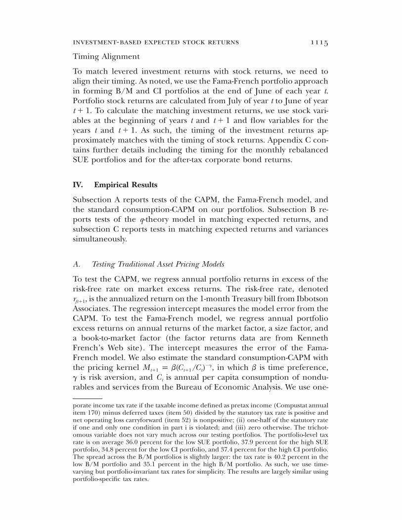
TABLE 1Descriptive Statistics of Testing Portfolio Returns

Low 5 High H�L m.a.e. [p]

A. 10 SUE PortfoliosSr̄i 10.9 19.0 23.4 12.5Sji 22.4 22.5 21.1 8.5

ei �1.7 6.6 10.9 12.6 5.7 [.0][�.7] [2.2] [5.0] [12.7]

FFei �4.6 2.0 9.5 14.1 4.0 [.0][�2.2] [1.0] [6.7] [8.1]

Cei �8.1 �.0 5.3 13.4 3.6 [.0][�1.3] [.0] [1.4] [.6]

B. 10 B/M PortfoliosSr̄i 8.7 17.9 25.8 17.1Sji 27.9 24.9 27.0 20.5

ei �4.9 5.2 13.7 18.6 6.3 [.0][�1.8] [2.3] [3.8] [6.0]

FFei �.5 1.8 6.8 7.3 2.8 [.0][�.2] [1.8] [2.6] [2.5]

Cei �5.4 .3 6.9 12.3 2.4 [.0][�.7] [.1] [2.4] [.2]

C. 10 CI PortfoliosSr̄i 22.1 18.1 15.2 �7.0Sji 32.4 22.3 26.7 11.4

ei 8.2 5.9 1.9 �6.3 5.7 [.0][2.4] [2.6] [.7] [�4.5]

FFei 6.5 1.5 .1 �6.3 2.2 [.0][2.9] [1.6] [.1] [�6.5]

Cei 4.0 .5 �4.3 �8.4 1.8 [.0][.7] [.1] [�.8] [�.4]

Note.—For testing portfolio i, we report in annual percent the average stock return, , the stock return volatility,Sr̄i

, the intercept from the CAPM regression, , the intercept from the Fama-French three-factor regression, , and theS FFj e ei i i

model error from the standard consumption-CAPM, . In each panel we report results for only three (low, 5, andCei

high) out of 10 portfolios to save space. The H–L portfolio is long in the high portfolio and short in the low portfolio.The heteroscedasticity- and autocorrelation-consistent t-statistics for the model errors are reported in brackets beneaththe corresponding errors. m.a.e. is the mean absolute error in annual percent for a given set of 10 testing portfolios.For the CAPM and the Fama-French model, the p-values in brackets in the last column in each panel are for the Gibbonset al. (1989) tests of the null hypothesis that the intercepts for a given set of 10 portfolios are jointly zero. For theconsumption-CAPM the p-values are for the test from one-stage GMM that the moment restrictions for all 10 portfolios2xare jointly zero. In panel A for the consumption-CAPM the estimate of the time preference coefficient is b p 2.8(standard error 0.9) and the estimate of risk aversion is (54.9). In panel B (1.2) andg p 127.6 b p 3.3 g p 142.1(58.5). In panel C (1.2) and (57.6).b p 3.3 g p 143.3

stage GMM with the identity weighting matrix to estimate the moments. We also include as an addi-SE[M (r � r )] p 0 E[M r ] p 1t�1 it�1 ft�1 t�1 ft�1

tional moment condition to identify b. The error of the standard con-sumption-CAPM is calculated as .SE [M (r � r )]/E [M ]T t�1 it�1 ft�1 T t�1

The SUE, B/M, and CI effects cannot be captured by the traditionalmodels. Panel A of table 1 shows that from the low SUE to the highSUE portfolio the average return increases monotonically from 10.9percent to 23.4 percent per year. The portfolio volatilities are largelyflat at around 22 percent. The CAPM error of the high-minus-low SUE


portfolio is 12.6 percent per year ( ), and the (annualized)t p 12.7mean absolute error, denoted m.a.e., is 5.7 percent. The Gibbons, Ross,and Shanken (1989) statistic, which tests the null hypothesis that allthe 10 individual intercepts are jointly zero, rejects the CAPM. (Theintercepts do not add up to zero because we equal-weight the portfolioreturns.) The performance of the Fama-French model is similar: them.a.e. is 4.0 percent per year and the Gibbons et al. test rejects themodel. The error of the high-minus-low SUE portfolio from the Fama-French model is 14.1 percent per year ( ). The consumption-t p 8.1CAPM error increases from �8.1 percent for the low SUE portfolioto 5.3 percent per year for the high SUE portfolio. Although the errorsare not individually significant, probably because of large measure-ment errors in consumption data, the test rejects the null hypothesis2x

that the pricing errors are jointly zero at the 1 percent significancelevel. In addition, the parameter estimates are high: the time pref-erence estimate is 2.8, and the risk aversion estimate is 127.6.

Panel B of table 1 shows that value stocks with high B/M ratios earnhigher average stock returns than growth stocks with low B/M ratios,25.8 percent versus 8.7 percent per year. The difference of 17.1 percentis significant ( ). There is no discernible relation between B/Mt p 5.5and stock return volatility: both the value and the growth portfolios havevolatilities around 27 percent. The CAPM error increases monotonicallyfrom �4.9 percent for growth stocks to 13.7 percent for value stocks.The average magnitude of the errors is 6.3 percent per year, and theGibbons et al. test strongly rejects the CAPM. Even the Fama-Frenchmodel fails to capture the equal-weighted returns: the high-minus-lowportfolio has an error of 7.3 percent ( ). The consumption-CAPMt p 2.5error increases from �5.4 percent for growth stocks to 6.9 percent forvalue stocks with an average magnitude of 2.4 percent, and the modelis rejected by the test.2x

From panel C, high CI stocks earn lower average stock returns thanlow CI stocks: 15.2 percent versus 22.1 percent per year, and the dif-ference is more than four standard errors from zero. The high-minus-low CI portfolio has an error of �6.3 percent ( ) from the CAPMt p �4.5and an error of �6.3 percent ( ) from the Fama-French model.t p �6.5Both models are rejected by the Gibbons et al. test. The consumption-CAPM error decreases from 4.0 percent for the low CI portfolio to �4.3percent for the high CI portfolio with an average magnitude of 1.8percent, and the test rejects the model.2x


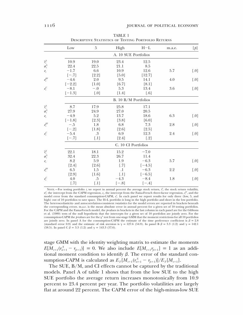
TABLE 2Parameter Estimates and Tests of Overidentification

SUE B/M CI

A. Matching Expected Returns

a 7.7 22.3 1.0[1.7] [25.5] [.3]

a .3 .5 .2[.0] [.3] [.0]

x2 4.4 6.0 6.5d.f. 8 8 8p .8 .7 .6m.a.e. .7 2.3 1.5

B. Matching Expected Returns andVariances

a 28.9 11.5 16.2[16.3] [4.8] [5.5]

a .6 .4 .4[.3] [.1] [.1]

2x(2) 5.1 6.2 6.1d.f.(2) 8 8 8p(2) .7 .6 .6m.a.e.(2)#100 2.5 4.1 2.2

2x(1) 5.2 4.4 4.8d.f.(1) 8 8 8p(1) .7 .8 .8m.a.e.(1) 3.5 2.6 2.2x2 5.5 6.2 6.6d.f. 18 18 18p 1.0 1.0 1.0

Note.—Results are from one-stage GMM with an identity weighting matrix. Inpanel A the moment conditions are . a is the adjustment cost pa-S IwE[r � r ] p 0it�1 it�1

rameter, and a is capital’s share. Their standard errors are in brackets beneath theestimates. , d.f., and p are the statistic, the degrees of freedom, and the p-value2xtesting that the moment conditions are jointly zero, respectively. m.a.e. is the meanabsolute error in annual percent, , in which is the sample mean,S IwE [r � r ] ET it�1 it�1 T

across a given set of testing portfolios. In panel B the moment conditions areand . , d.f.(2), andS Iw S S 2 Iw Iw 2 2E[r � r ] p 0 E[(r � E[r ]) � (r � E[r ]) ] p 0 xit�1 it�1 it�1 it�1 it�1 it�1 (2)

are the statistic, degrees of freedom, and p-value for the test that the variance2p(2) xerrors, defined as , are jointly zero. m.a.e.(2)S S 2 Iw Iw 2E [(r � E [r ]) � (r � E [r ]) ]T it�1 T it�1 it�1 T it�1

is the mean absolute variance error. , d.f.(1), and are the statistic, degrees2x p(1)(1)

of freedom, and p-value for the test that the expected return errors are jointly2xzero. m.a.e.(1) is the mean absolute expected return error in annual percent. ,2xd.f., and p are the statistic, degrees of freedom, and p-value of the test that the expectedreturn errors and the variance errors are jointly zero.

B. The q-Theory Model: Matching Expected Returns

Point Estimates and Overall Model Performance

We estimate only two parameters in our parsimonious model: the ad-justment cost parameter, a, and capital’s share, a. Panel A of table 2provides estimates of a ranging from 0.2 to 0.5. These estimates arelargely comparable to the approximate 0.3 figure for capital’s share inRotemberg and Woodford (1992). The estimates of a are not as stableacross the different sets of testing portfolios. We find significant esti-


mates of 7.7 and 1.0 for the SUE and CI portfolios, respectively. Theestimate is 22.3 for the B/M portfolios but with a high standard errorof 25.5. These estimates fall within the wide range of estimates fromstudies using quantity data. The evidence implies that firms’ optimiza-tion problem has an interior solution: the positive estimates of a meanthat the adjustment cost function is increasing and convex in .Iit

Panel A of table 2 also reports two measures of overall model per-formance: the mean absolute error, m.a.e., and the test. The model2x

does a good job in accounting for the average returns of the 10 SUEportfolios. The m.a.e. is 0.7 percent per year, which is lower than thosefrom the CAPM, 5.7 percent, the Fama-French model, 4.0 percent, andthe standard consumption-CAPM, 3.6 percent. Unlike the traditionalmodels that are rejected using the SUE portfolios, the q-theory modelis not rejected by the test. The overall performance of the model is2x

more modest in capturing the average B/M portfolio returns. Althoughthe model is not formally rejected by the test, the m.a.e. is 2.3 percent2x

per year, which is comparable to that from the Fama-French model, 2.8percent, and that from the standard consumption-CAPM, 2.4 percent,but is lower than that from the CAPM, 6.3 percent. The model doesbetter in pricing the 10 CI portfolios. The m.a.e. is 1.5 percent per year,which is lower than those from the CAPM, 5.7 percent, the Fama-Frenchmodel, 2.2 percent, and the standard consumption-CAPM, 1.8 percent.The q-theory model is again not rejected by the test.2x

Euler Equation Errors

The m.a.e.’s and tests indicate only overall model performance. To2x

provide a more complete picture, we report each individual portfolioerror, , defined in equation (8), in which levered investment returnsqei

are constructed using the estimates from panel A of table 2. We alsoreport the t-statistic, described in Appendix B, testing that an individualerror equals zero.

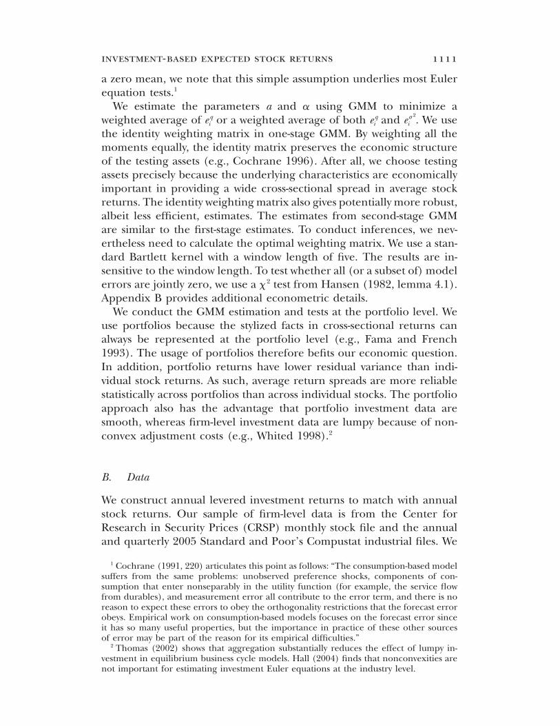
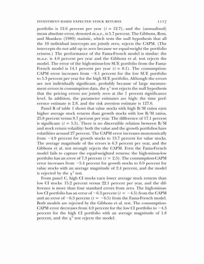
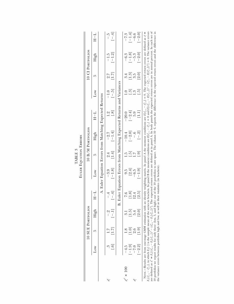
The magnitude of the individual errors varies from 0.1 percent to 1.7percent per year across 10 SUE portfolios, and none of the errors aresignificant. In particular, panel A of table 3 shows that the high-minus-low SUE portfolio has an error of �0.4 percent per year ( ).t p �0.4This error is negligible compared to the large errors from the traditionalmodels: 12.6 percent for the CAPM, 14.1 percent for the Fama-Frenchmodel, and 13.4 percent for the standard consumption-CAPM. Figure1 offers a visual presentation of the fit. Figure 1a plots the averagelevered investment returns of the 10 SUE portfolios against their averagestock returns. If the model performs perfectly, all the observationsshould lie on the 45-degree line. From figure 1a, the scatter plot fromthe q-theory model is largely aligned with the 45-degree line. The re-

TA

BL

E3

Eu

ler

Eq

uat

ion

Err

ors

10SU

EPo

rtfo

lio

s10

B/M

Port

foli

os

10C

IPo

rtfo

lio

s

Low

5H

igh

H�

LL

ow5

Hig

hH

�L

Low

5H

igh

H�

L

A.

Eul

erE

quat

ion

Err

ors

from

Mat

chin

gE

xpec

ted

Ret

urn

sq e i

.31.

7�

.2�

.4�

3.9

2.4

�2.

71.

2�

1.0

2.7

�1.

5�

.5[.

6][1

.7]

[�.1

][�

.4]

[�1.

8][1

.4]

[�1.

4][.

8][�

.5]

[1.7

][�

1.2]

[�.4

]

B.

Eul

erE

quat

ion

Err

ors

from

Mat

chin

gE

xpec

ted

Ret

urn

san

dV

aria

nce

s2

j e#

100

i�

4.5

1.8

3.1

7.6

9.5

1.5

�10

.4�

20.0

1.0

3.4

�6.

3�

7.3

[�1.

9][1

.0]

[1.5

][1

.8]

[2.4

][.

5][�

2.0]

[�2.

4][.

3][1

.3]

[�1.

8][�

1.4]

q e i�

7.0

2.6

5.4

12.4

�6.

51.

7�

.65.

91.

33.

5�

5.3

�6.

6[�

2.2]

[1.9

][2

.0]

[2.5

][�

1.9]

[.9]

[�.2

][1

.1]

[.5]

[2.0

][�

2.0]

[�2.

0]

No

te.—

Res

ults

are

from

one-

stag

eG

MM

esti

mat

ion

wit

han

iden

tity

wei

ghti

ng

mat

rix.

Inpa

nel

Ath

em

omen

tco

ndi

tion

sar

e.

Th

eex

pect

edre

turn

erro

rsar

ede

fin

edas

SIw

qE[

r�

r]

p0

e{

it�

1it�

1i

,in

wh

ich

isth

esa

mpl

em

ean

ofth

ese

ries

inbr

acke

ts.I

npa

nel

Bth

em

omen

tco

ndi

tion

sar

ean

d.T

he

vari

ance

erro

rsS

IwS

IwS

S2

IwIw

2E

[r�

r]

E[7

]E[

r�

r]

p0

E[(r

�E[

r])

�(r

�E[

r])

]p

0T

it�

1it�

1T

it�

1it�

1it�

1it�

1it�

1it�

1

are

defi

ned

as.

Th

eex

pect

edre

turn

erro

rsar

ede

fin

edas

inpa

nel

A.

Inbo

thpa

nel

sth

eex

pect

edre

turn

erro

rsar

ein

ann

ual

perc

ent.

Inea

chse

tof

2j

SS

2Iw

Iw2

e{

E[(

r�

E[r

])�

(r�

E[r

])]

iT

it�

1T

it�

1it�

1T

it�

1

10po

rtfo

lios

we

repo

rtre

sult

sfo

ron

lyth

ree

(low

,5,

and

hig

h)

out

ofth

e10

port

folio

sto

save

spac

e.T

he

colu

mn

H�

Lre

port

sth

edi

ffer

ence

inth

eex

pect

edre

turn

erro

rsan

dth

edi

ffer

ence

inth

eva

rian

ceer

rors

betw

een

port

folio

sh

igh

and

low,

asw

ell

asth

eir

t-sta

tist

ics

(in

brac

kets

).


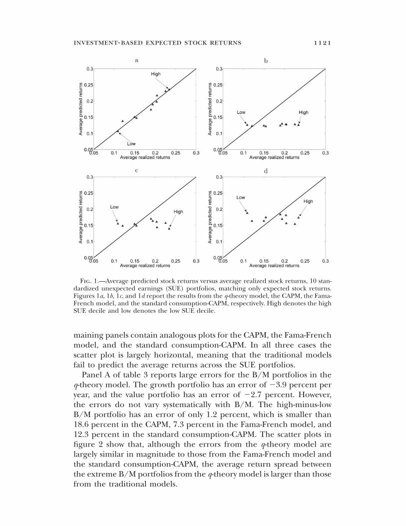
Fig. 1.—Average predicted stock returns versus average realized stock returns, 10 stan-dardized unexpected earnings (SUE) portfolios, matching only expected stock returns.Figures 1a, 1b, 1c, and 1d report the results from the q-theory model, the CAPM, the Fama-French model, and the standard consumption-CAPM, respectively. High denotes the highSUE decile and low denotes the low SUE decile.

maining panels contain analogous plots for the CAPM, the Fama-Frenchmodel, and the standard consumption-CAPM. In all three cases thescatter plot is largely horizontal, meaning that the traditional modelsfail to predict the average returns across the SUE portfolios.

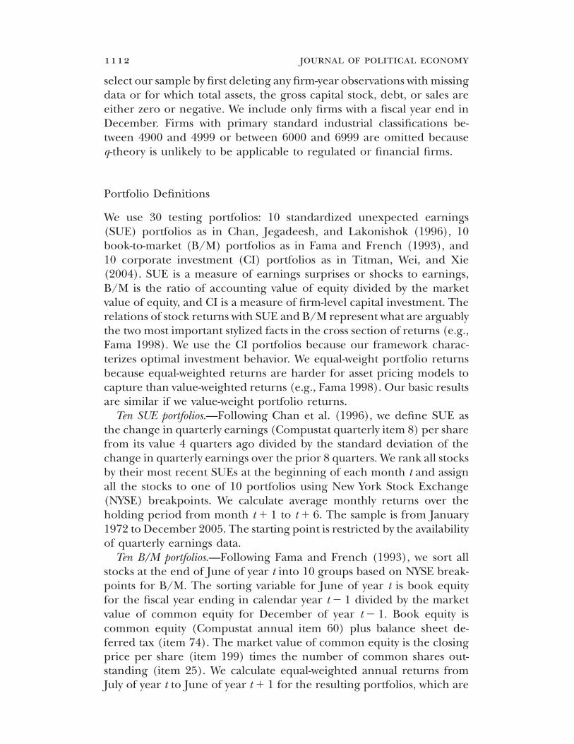
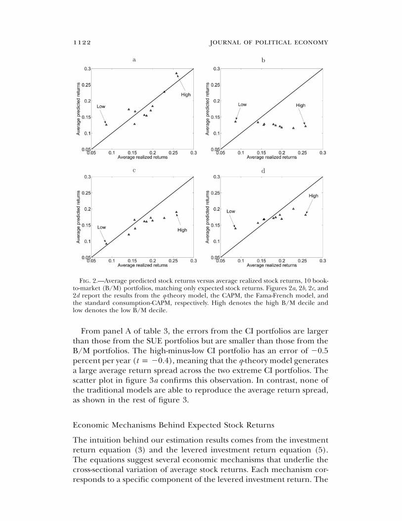
Panel A of table 3 reports large errors for the B/M portfolios in theq-theory model. The growth portfolio has an error of �3.9 percent peryear, and the value portfolio has an error of �2.7 percent. However,the errors do not vary systematically with B/M. The high-minus-lowB/M portfolio has an error of only 1.2 percent, which is smaller than18.6 percent in the CAPM, 7.3 percent in the Fama-French model, and12.3 percent in the standard consumption-CAPM. The scatter plots infigure 2 show that, although the errors from the q-theory model arelargely similar in magnitude to those from the Fama-French model andthe standard consumption-CAPM, the average return spread betweenthe extreme B/M portfolios from the q-theory model is larger than thosefrom the traditional models.


Fig. 2.—Average predicted stock returns versus average realized stock returns, 10 book-to-market (B/M) portfolios, matching only expected stock returns. Figures 2a, 2b, 2c, and2d report the results from the q-theory model, the CAPM, the Fama-French model, andthe standard consumption-CAPM, respectively. High denotes the high B/M decile andlow denotes the low B/M decile.

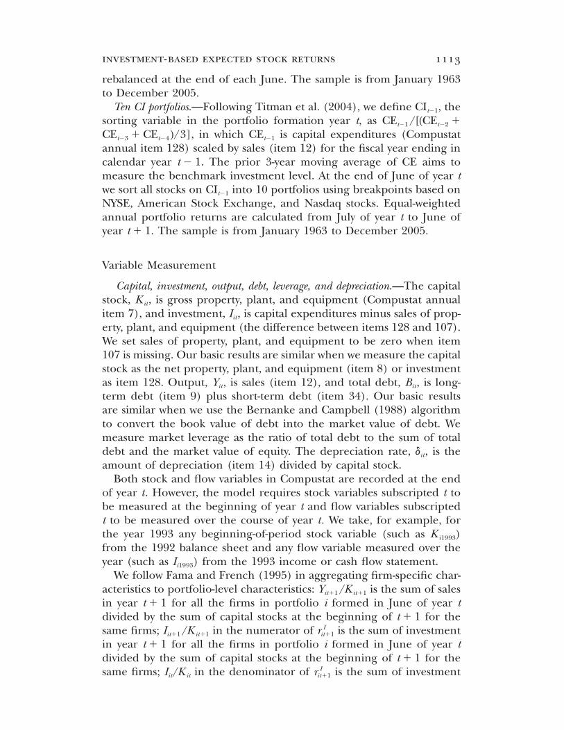
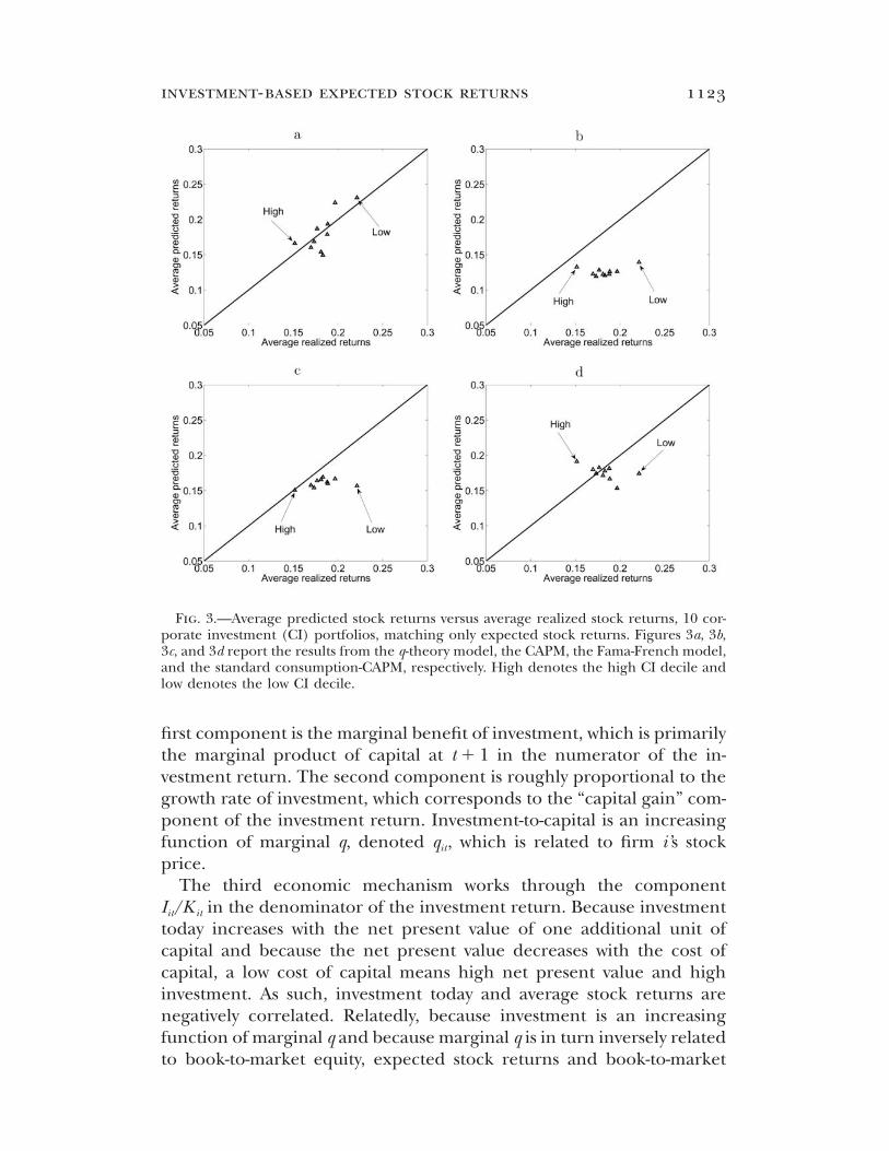
From panel A of table 3, the errors from the CI portfolios are largerthan those from the SUE portfolios but are smaller than those from theB/M portfolios. The high-minus-low CI portfolio has an error of �0.5percent per year ( ), meaning that the q-theory model generatest p �0.4a large average return spread across the two extreme CI portfolios. Thescatter plot in figure 3a confirms this observation. In contrast, none ofthe traditional models are able to reproduce the average return spread,as shown in the rest of figure 3.

Economic Mechanisms Behind Expected Stock Returns

The intuition behind our estimation results comes from the investmentreturn equation (3) and the levered investment return equation (5).The equations suggest several economic mechanisms that underlie thecross-sectional variation of average stock returns. Each mechanism cor-responds to a specific component of the levered investment return. The


Fig. 3.—Average predicted stock returns versus average realized stock returns, 10 cor-porate investment (CI) portfolios, matching only expected stock returns. Figures 3a, 3b,3c, and 3d report the results from the q-theory model, the CAPM, the Fama-French model,and the standard consumption-CAPM, respectively. High denotes the high CI decile andlow denotes the low CI decile.

first component is the marginal benefit of investment, which is primarilythe marginal product of capital at in the numerator of the in-t � 1vestment return. The second component is roughly proportional to thegrowth rate of investment, which corresponds to the “capital gain” com-ponent of the investment return. Investment-to-capital is an increasingfunction of marginal q, denoted , which is related to firm i’s stockqit

price.The third economic mechanism works through the component

in the denominator of the investment return. Because investmentI /Kit it

today increases with the net present value of one additional unit ofcapital and because the net present value decreases with the cost ofcapital, a low cost of capital means high net present value and highinvestment. As such, investment today and average stock returns arenegatively correlated. Relatedly, because investment is an increasingfunction of marginal q and because marginal q is in turn inversely relatedto book-to-market equity, expected stock returns and book-to-market


equity are positively correlated. The fourth component is the rate ofdepreciation, . Collecting terms involving in the numerator ofd dit�1 it�1

equation (3) yields , meaning that high�(1 � t )[1 � a(I /K )]dt�1 it�1 it�1 it�1

rates of depreciation tomorrow imply lower average returns. The fifthcomponent is market leverage: taking the first-order derivative of equa-tion (5) with respect to shows that expected stock returns shouldwit

increase with market leverage today.In short, all else equal, firms should earn lower average stock returns

if they have high investment-to-capital today, low expected investmentgrowth, low sales-to-capital tomorrow, high rates of depreciation to-morrow, or low market leverage today.

Expected Returns Accounting

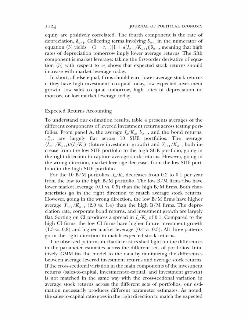
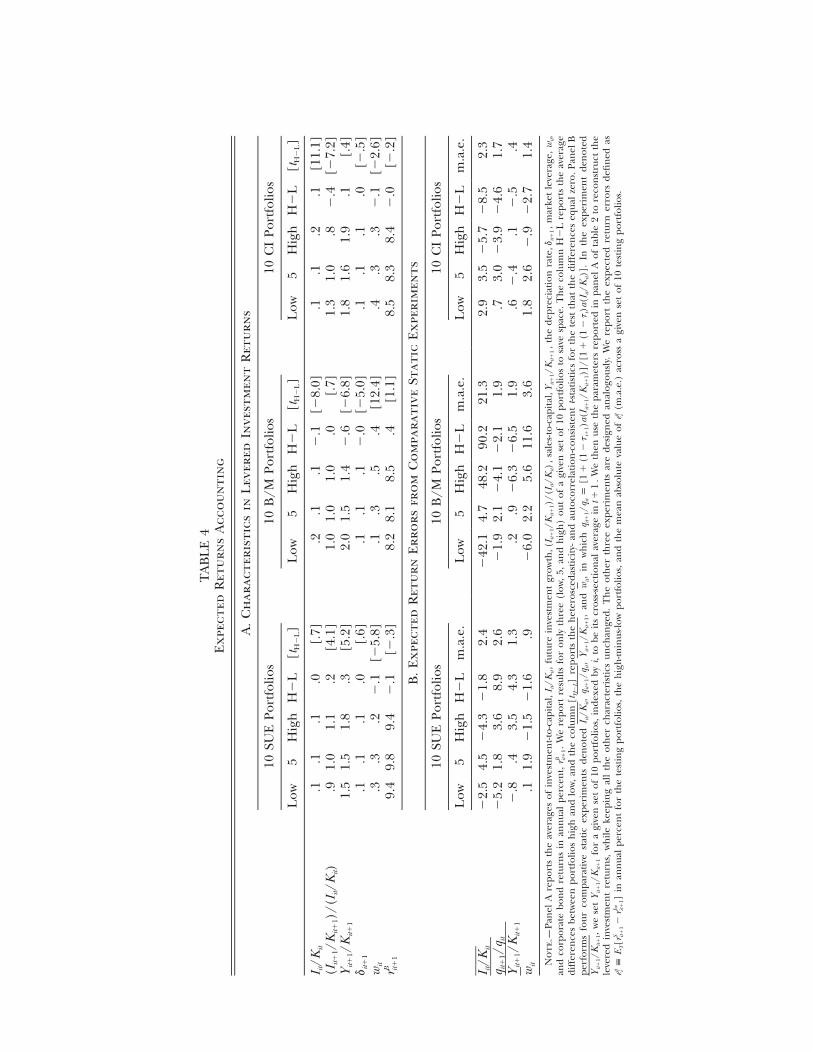
To understand our estimation results, table 4 presents averages of thedifferent components of levered investment returns across testing port-folios. From panel A, the average , , and the bond returns,I /K dit it it�1

, are largely flat across 10 SUE portfolios. The averageBrit�1

(future investment growth) and both in-(I /K )/(I /K ) Y /Kit�1 it�1 it it it�1 it�1

crease from the low SUE portfolio to the high SUE portfolio, going inthe right direction to capture average stock returns. However, going inthe wrong direction, market leverage decreases from the low SUE port-folio to the high SUE portfolio.

For the 10 B/M portfolios, decreases from 0.2 to 0.1 per yearI /Kit it

from the low to the high B/M portfolio. The low B/M firms also havelower market leverage (0.1 vs. 0.5) than the high B/M firms. Both char-acteristics go in the right direction to match average stock returns.However, going in the wrong direction, the low B/M firms have higheraverage (2.0 vs. 1.4) than the high B/M firms. The depre-Y /Kit�1 it�1

ciation rate, corporate bond returns, and investment growth are largelyflat. Sorting on CI produces a spread in of 0.1. Compared to theI /Kit it

high CI firms, the low CI firms have higher future investment growth(1.3 vs. 0.8) and higher market leverage (0.4 vs. 0.3). All three patternsgo in the right direction to match expected stock returns.

The observed patterns in characteristics shed light on the differencesin the parameter estimates across the different sets of portfolios. Intu-itively, GMM fits the model to the data by minimizing the differencesbetween average levered investment returns and average stock returns.If the cross-sectional variation in the main components of the investmentreturns (sales-to-capital, investment-to-capital, and investment growth)is not matched in the same way with the cross-sectional variation inaverage stock returns across the different sets of portfolios, our esti-mation necessarily produces different parameter estimates. As noted,the sales-to-capital ratio goes in the right direction to match the expected

TA

BL

E4

Ex

pect

edR

etu

rns

Acc

ou

nti

ng

A.

Ch

arac

teri

stic

sin

Lev

ered

Inve

stm

ent

Ret

urn

s

10SU

EPo

rtfo

lios

10B

/MPo

rtfo

lios

10C

IPo

rtfo

lios

Low

5H

igh

H�

L[t

H�

L]

Low

5H

igh

H�

L[t

H�

L]

Low

5H

igh

H�

L[t

H�

L]

I/K

itit

.1.1

.1.0

[.7]

.2.1

.1�

.1[�

8.0]

.1.1

.2.1

[11.

1](I

/K)/

(I/K

)it�

1it�

1it

it.9

1.0

1.1

.2[4

.1]

1.0

1.0

1.0

.0[.

7]1.

31.

0.8

�.4

[�7.

2]Y

/Kit�

1it�

11.

51.

51.

8.3

[5.2

]2.

01.

51.

4�

.6[�

6.8]

1.8

1.6

1.9

.1[.

4]d i

t�1

.1.1

.1.0

[.6]

.1.1

.1�

.0[�

5.0]

.1.1

.1.0

[�.5

]w

it.3

.3.2

�.1

[�5.

8].1

.3.5

.4[1

2.4]

.4.3

.3�

.1[�

2.6]

B r it�

19.

49.

89.

4�

.1[�

.3]

8.2

8.1

8.5

.4[1

.1]

8.5

8.3

8.4

�.0

[�.2

]

B.

Ex

pect

edR

etu

rnE

rro

rsfr

om

Co

mpa

rati

veSt

atic

Ex

peri

men

ts

10SU

EPo

rtfo

lios

10B

/MPo

rtfo

lios

10C

IPo

rtfo

lios

Low

5H

igh

H�

Lm

.a.e

.L

ow5

Hig

hH

�L

m.a

.e.

Low

5H

igh

H�

Lm

.a.e

.

I/K

itit

�2.

54.

5�

4.3

�1.

82.

4�

42.1

4.7

48.2

90.2

21.3

2.9

3.5

�5.

7�

8.5

2.3

q/q

it�

1it

�5.

21.

83.

68.

92.

6�

1.9

2.1

�4.

1�

2.1

1.9

.73.

0�

3.9

�4.

61.

7Y

/Kit�

1it�

1�

.8.4

3.5

4.3

1.3

.2.9

�6.

3�

6.5

1.9

.6�

.4.1

�.5

.4w

it.1

1.9

�1.

5�

1.6

.9�

6.0

2.2

5.6

11.6

3.6

1.8

2.6

�.9

�2.

71.

4

No

te.—

Pan

elA

repo

rts

the

aver

ages

ofin

vest

men

t-to-

capi

tal,

,fu

ture

inve

stm

ent

grow

th,

,sa

les-

to-c

apit

al,

,th

ede

prec

iati

onra

te,

,mar

ket

leve

rage

,,

I/K

(I/K

)/(I

/K)

Y/K

dw

itit

it�

1it�

1it

itit�

1it�

1it�

1it

and

corp

orat

ebo

nd

retu

rns

inan

nua

lpe

rcen

t,.

We

repo

rtre

sult

sfo

ron

lyth

ree

(low

,5,

and

hig

h)

out

ofa

give

nse

tof

10po

rtfo

lios

tosa

vesp

ace.

Th

eco

lum

nH

�L

repo

rts

the

aver

age

B r it�

1

diff

eren

ces

betw

een

port

folio

sh

igh

and

low,

and

the

colu

mn

repo

rts

the

het

eros

ceda

stic

ity-

and

auto

corr

elat

ion

-con

sist

ent

t-sta

tist

ics

for

the

test

that

the

diff

eren

ces

equa

lzer

o.Pa

nel

B[t

]H

�L

perf

orm

sfo

urco

mpa

rati

vest

atic

expe

rim

ents

den

oted

,,

,an

d,

inw

hic

h.

Inth

eex

peri

men

tde

not

edI

/Kq

/qY

/Kw

q/q

p[1

�(1

�t

)a(I

/K)]

/[1

�(1

�t

)a(I

/K)]

itit

it�

1it

it�

1it�

1it�

1it

t�1

it�

1it�

1t

itit

it

,w

ese

tfo

ra

give

nse

tof

10po

rtfo

lios,

inde

xed

byi,

tobe

its

cros

s-se

ctio

nal

aver

age

in.

We

then

use

the

para

met

ers

repo

rted

inpa

nel

Aof

tabl

e2

tore

con

stru

ctth

eY

/KY

/Kt�

1it�

1it�

1it�

1it�

1

leve

red

inve

stm

ent

retu

rns,

wh

ileke

epin

gal

lth

eot

her

char

acte

rist

ics

unch

ange

d.T

he

oth

erth

ree

expe

rim

ents

are

desi

gned

anal

ogou

sly.

We

repo

rtth

eex

pect

edre

turn

erro

rsde

fin

edas

inan

nua

lpe

rcen

tfo

rth

ete

stin

gpo

rtfo

lios,

the

hig

h-m

inus

-low

port

folio

s,an

dth

em

ean

abso

lute

valu

eof

(m.a

.e.)

acro

ssa

give

nse

tof

10te

stin

gpo

rtfo

lios.

qS

Iwq

e{

E[r

�r

]e

iT

it�

1it�

1i


returns of the SUE portfolios but goes in the wrong direction to matchthe expected returns of the B/M portfolios. The different estimatesimply different economic mechanisms underlying the cross section ofexpected returns across the different sets of portfolios.

To quantify the role of each component of the investment return inmatching expected returns, we conduct the following accounting ex-ercises. We set a given component equal to its cross-sectional averagein each year. We then use the parameter estimates in panel A of table2 to reconstruct levered investment returns, while keeping all the othercharacteristics unchanged. In the case of investment growth, we holdconstant the capital gain component of the investment return, whichis given by

1 � (1 � t )a(I /K ) qt�1 it�1 it�1 it�1p . (10)1 � (1 � t)a(I /K ) qt it it it

We focus on the resulting change in the magnitude of the expectedreturn errors: a large change would suggest that the component inquestion is quantitatively important.

Panel B of table 4 reports several insights. First, the most importantcomponent for the SUE portfolio returns is : eliminating its cross-q /qit�1 it

sectional variation makes the q-theory model underpredict the averagestock return of the high-minus-low SUE portfolio by 8.9 percent peryear. In contrast, this error is only �0.4 percent in the benchmarkestimation. Without the cross-sectional variation of , the errorY /Kit�1 it�1

of the high-minus-low SUE portfolio becomes 4.3 percent. Second, in-vestment and leverage are both important for the B/M portfolios. Fixing

to its cross-sectional average produces an error of 90.2 percentI /Kit it

per year for the high-minus-low B/M portfolio. This huge error reflectsthe large estimate of the parameter a for the B/M portfolios. Setting

to its cross-sectional average produces an error of 11.6 percent forwit

the high-minus-low B/M portfolio. The terms and areY /K q /qit�1 it�1 it�1 it

less important. Third, the dominating force in driving the average stockreturns across the CI portfolios is . Eliminating its cross-sectionalI /Kit it

variation gives rise to an error of �8.5 percent per year for the high-minus-low CI portfolio. Fixing produces an error of 4.6 percent,q /qit�1 it

and fixing produces an error of 2.7 percent per year. The effect ofwit

is negligible.Y /Kit�1 it�1

C. Matching Expected Returns and Variances Simultaneously

Point Estimates and Overall Model Performance

Panel B of table 2 reports the point estimates and overall model per-formance when we use the q-theory model to match both the expected


returns and variances of the testing portfolios. Capital’s share, a, isestimated from 0.4 to 0.6, and all estimates are significant. The estimatesof the adjustment cost parameter, a, are on average higher than thosereported in panel A. The estimates are 11.5 and 16.2 for the B/M andCI portfolios, and both are significant. The estimate of a for the SUEportfolios is 28.9, but with a large standard error of 16.3.

As explained in Erickson and Whited (2000), it can be misleading tointerpret the parameter a in terms of adjustment costs or speeds. Wefollow their suggestion of gauging the economic magnitude of this pa-rameter in terms of the elasticity of investment with respect to marginalq. Evaluated at the sample mean, this elasticity is given by times the1/aratio of the mean of to the mean of . The estimates in panel Bq I /Kit it it

imply elasticities that range from 0.4 to 0.7. A similar inelastic responseof 0.1 is implied by the estimate of a for the B/M portfolios in panelA. However, the implied elasticity for the SUE portfolios is greater thanone, and that for the CI portfolios is over 10. Although this last estimateseems large, the others fall in a reasonable range between zero and 1.3.The general inference is that investment responds to q inelastically.

Panel B of table 2 reports three tests of overall model performance:is the test that all the variance errors are jointly zero, is the2 2 2x x x(2) (1)

test that all the expected return errors are jointly zero, and the statistic2x

labeled tests that all the model errors are jointly zero. The tests2 2x x(2)

do not reject the model, and the mean absolute variance errors, denotedm.a.e.(2), are small. To better interpret their economic magnitude, weuse the parameter estimates from panel B of table 2 to calculate theaverage levered investment return volatility (instead of variance). At 20.4percent, this average predicted volatility is close to the average realizedvolatility, 21.1 percent, across the 10 SUE portfolios. For the 10 B/Mportfolios, the average stock return volatility is 25.0 percent, and theaverage levered investment return volatility is 23.6 percent. Finally, forthe 10 CI portfolios the average stock return volatility is 24.8 percent,and their average levered investment return volatility is 24.4 percent.

Cochrane (1991) reports that the aggregate investment return vola-tility is only about 60 percent of the value-weighted stock market vola-tility. Our results complement Cochrane’s in several ways. First, weaccount for leverage, whereas Cochrane does not. Second, we use port-folios as testing assets, in which firm-specific shocks are unlikely to bediversified away entirely, whereas Cochrane studies the stock marketportfolio. Third, we formally choose parameters to match variances,whereas Cochrane calibrates his parameters to match expected returnsexactly but allows variances to vary.

Although the tests on the expected return errors do not reject2x(1)

the model, the mean absolute expected return errors, denotedm.a.e.(1), are large. The m.a.e.(1) for the SUE portfolios is 3.5 percent


per year, up from 0.7 percent when matching only expected returns.The m.a.e.(1) for the B/M portfolios increases from 2.3 percent to 2.6percent, whereas that for the CI portfolios goes up from 1.5 percent to2.2 percent. This increase is to be expected because we are asking moreof the model by matching more moments.

Euler Equation Errors

Panel B of table 3 reports individual variance errors, defined as in equa-tion (9), and expected return errors, defined as in equation (8), inwhich levered investment returns, , are constructed using the esti-Iwrit�1

mates from panel B of table 2. The t-statistics of the errors, describedin Appendix B, are calculated using the variance-covariance matrix fromone-stage GMM.

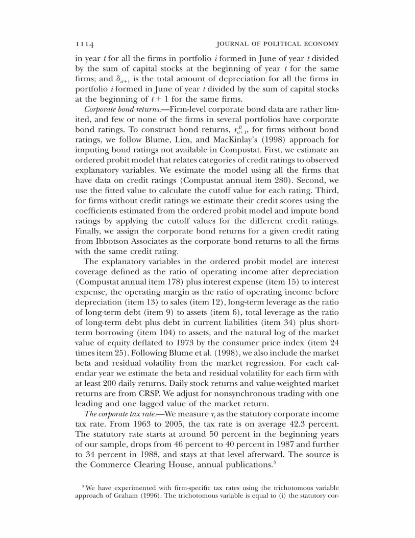
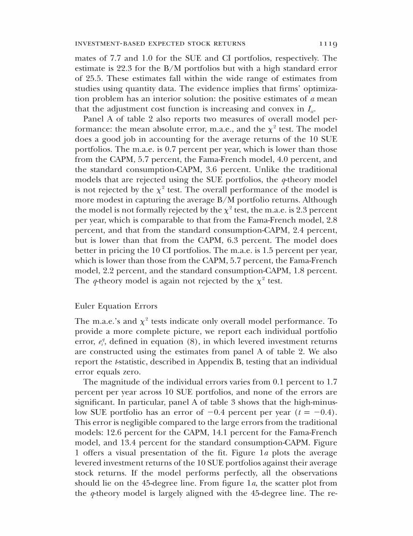
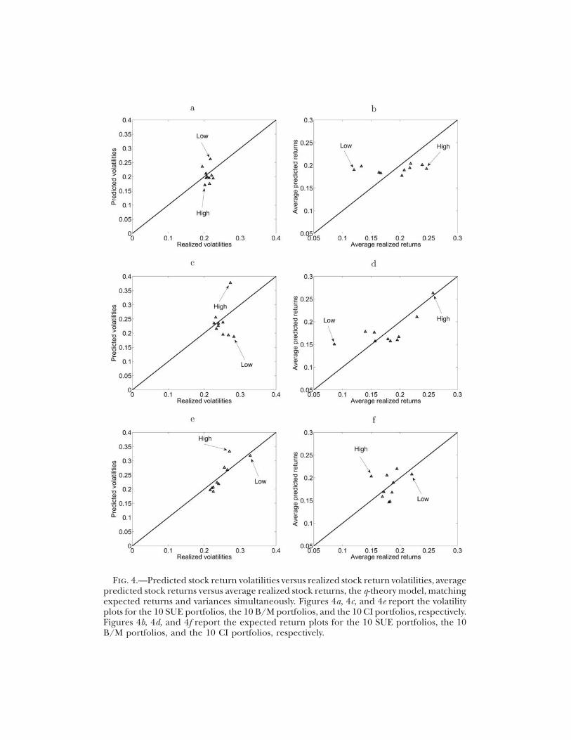
Panel B of table 3 shows that the magnitude of the variance errorsis small relative to stock return variances. Most variance errors are in-significant. The left panels in figure 4 plot levered investment returnvolatilities against stock return volatilities for the testing portfolios. (Tofacilitate interpretation, we plot volatilities instead of variances.) Thepoints in the scatter plot are generally aligned with the 45-degree line.However, while there is no discernible relation between stock returnvolatilities and the characteristics in the data, the model predicts a neg-ative relation between levered investment return volatilities and SUE(fig. 4a) and a positive relation between the predicted volatilities andB/M (fig. 4c). Panel B of table 3 also shows that the variance errorsincrease with SUE and decrease with B/M. The difference in the vari-ance errors is ( ) between the high and low SUE port-7.6/100 t p 1.8folios and is ( ) between the high and low B/M�20/100 t p �2.4portfolios.

Panel B of table 3 shows that the expected return errors vary system-atically with SUE, increasing from �7.0 percent per year for the lowSUE portfolio to 5.4 percent for the high SUE portfolio. The differenceof 12.4 percent ( ) is similar in magnitude to those from thet p 2.5traditional models. Figure 4b plots the average levered investment re-turns against the average stock returns. The pattern is largely horizontal,similar to those from the traditional models.

The expected return errors for the B/M portfolios in panel B of table3 also are larger than those in panel A from matching only expectedreturns. However, the model still predicts an average return spread of11.3 percent per year between the extreme B/M portfolios. The ex-pected return error for the high-minus-low B/M portfolio is 5.9 percentper year in the q-theory model, which is lower than 7.3 percent fromthe Fama-French model. The CAPM and the standard consumption-CAPM produce even higher errors, 18.6 percent and 12.3 percent, re-

Fig. 4.—Predicted stock return volatilities versus realized stock return volatilities, averagepredicted stock returns versus average realized stock returns, the q-theory model, matchingexpected returns and variances simultaneously. Figures 4a, 4c, and 4e report the volatilityplots for the 10 SUE portfolios, the 10 B/M portfolios, and the 10 CI portfolios, respectively.Figures 4b, 4d, and 4f report the expected return plots for the 10 SUE portfolios, the 10B/M portfolios, and the 10 CI portfolios, respectively.


spectively. The q-theory model’s performance in reproducing the av-erage returns of the CI portfolios deteriorates to the same level as inthe traditional models. The difference in the expected return errorsbetween the extreme CI portfolios is �6.6 percent, which is similar tothose from the CAPM and the Fama-French model. From figure 4f, thescatter plots of average returns from the q-theory model are largelyhorizontal.

The evidence shows that the q-theory model does a poor job of match-ing expected returns and variances simultaneously in the SUE and CIportfolios but a somewhat better job in the B/M portfolios. For the SUEand CI portfolios, when we match only expected returns, the predictedinvestment return variances are lower than observed stock return vari-ances because investment and output are not as volatile as stock returns.As such, to minimize model errors, the joint estimation of expectedreturns and variances produces empirically plausible variances by pick-ing large estimates of the adjustment cost parameter and of capital’sshare. These large estimates in turn cannot produce small expectedreturn errors. For the B/M portfolios, when we match only expectedreturns, the predicted variances are no longer low because of the highadjustment cost parameter estimate required to match expected returns.As such, the mean absolute expected return error does not deteriorateas much as it does in the case of the SUE and CI portfolios when wedo the joint estimation.

A Correlation Puzzle

As noted, equation (5), taken literally, predicts that stock returns shouldequal levered investment returns at every data point. We have so farexamined the first and second moments of returns that are the focusof much work in financial economics. We can explore yet another, evenstronger, prediction of the model: stock returns should be perfectlycorrelated with levered investment returns.

Table 5 reports that the contemporaneous time-series correlationsbetween stock and levered investment returns are weakly negative,whereas those between one-period-lagged stock returns and levered in-vestment returns are positive. When we pool all the observations in theSUE portfolios together, the contemporaneous correlation is �.1, whichis significant at the 5 percent level. However, the correlation betweenone-period-lagged stock returns and levered investment returns is .2,which is significant at the 1 percent level. Replacing levered investmentreturns with investment growth yields similar results, meaning that thecorrelations are insensitive to the investment return specifications.

Investment lags (lags between the decision to invest and the actualinvestment expenditure) can temporally shift the correlations between

TA

BL

E5

Co

rrel

atio

ns

A.

10SU

EPo

rtfo

lio

sB

.10

B/M

Port

foli

os

C.

10C

IPo

rtfo

lio

s

Low

5H

igh

All

Low

5H

igh

All

Low

5H

igh

All

SIw

r(r

,r

)it�

1it�

1�

.3�

.2�

.3�

.1**

�.2

�.2

�.1

�.1

**.2

�.3

**�

.3*

�.1

SIw

r(r

,r

)it

it�

1.2

.0.1

.2**

*.1

.2.3

***

.2**

*.4

***

.2.3

*.2

***

Sr(r

,I

/I)

it�

1it�

1it

�.3

�.2

�.2

�.1

�.1

�.1

�.1

�.2

***

�.3

*�

.3**

�.1

�.0

Sr(r

,I

/I)

itit�

1it

.2.0

�.0

.1**

.1.2

.3*

.1**

*.2

.1.3

.2**

*

No

te.—

We

repo

rtti

me-

seri

esco

rrel

atio

ns

ofst

ock

retu

rns

(con

tem

pora

neo

us,

,an

don

e-pe

riod

-lagg

ed,

)w

ith

leve

red

inve

stm

ent

retu

rns,

,an

dw

ith

inve

stm

ent

grow

th,

.In

each

SS

Iwr

rr

I/I

it�

1it

it�

1it�

1it

pan

elw

ere

port

resu

lts

for

only

thre

e(l

ow,5

,an

dh

igh

)ou

tof

10po

rtfo

lios

tosa

vesp

ace.

den

otes

the

corr

elat

ion

betw

een

the

two

seri

esin

the

pare

nth

eses

.In

the

last

colu

mn

ofea

chpa

nel

r(7

,7)

(all)

we

repo

rtth

eco

rrel

atio

ns

and

thei

rsi

gnifi

can

ceby

pool

ing

all

the

obse

rvat

ion

sfo

ra

give

nse

tof

10te

stin

gpo

rtfo

lios.

Th

ele

vere

din

vest

men

tre

turn

sar

eco

nst

ruct

edus

ing

the

para

met

ers

inpa

nel

Aof

tabl

e2.

*Si

gnifi

can

tat

the

10pe

rcen

tle

vel.

**Si

gnifi

can

tat

the

5pe

rcen

tle

vel.

***

Sign

ifica

nt

atth

e1

perc

ent

leve

l.


investment growth and stock returns (e.g., Lamont 2000). Lags preventfirms from adjusting investment immediately in response to discountrate changes. Consider a 1-year lag. A discount rate fall in year t increasesinvestment only in year . When stock returns rise in year t (becauset � 1of the discount rate fall), investment growth rises in year : laggedt � 1stock returns should be positively correlated with investment growth.The discount rate fall in year t also means low average stock returns inyear , coinciding with high investment growth in year . As such,t � 1 t � 1the contemporaneous correlation between stock returns and investmentgrowth should be negative. These lead-lag correlations are consistentwith the evidence in table 5.

V. Conclusion

We use GMM to estimate a structural model of cross-sectional stockreturns derived from the q-theory of investment. The model is parsi-monious with only two parameters. We construct empirical first- andsecond-moment conditions based on the q-theory prediction that stockreturns equal levered investment returns. The latter can be constructedfrom firm characteristics. When matching the first moments only, themodel captures the average stock returns of portfolios sorted by earningssurprises, book-to-market equity, and capital investment. When match-ing the first and the second moments simultaneously, the volatilitiesfrom the model are empirically plausible, but the resulting expectedreturns errors are large. Finally, the model also falls short in reproducingthe correlation structure between stock returns and investment growth.We conclude that, on average, portfolios of firms do a good job ofaligning investment policies with their costs of capital and that thisalignment drives many stylized facts in cross-sectional returns. However,because we do not parameterize the stochastic discount factor, our workis silent about why average return spreads across characteristics-sortedportfolios are not matched with spreads in covariances empirically.

Appendix A

Proof of Proposition 1

Let be the Lagrangian multiplier associated with . Theq K p I � (1 � d )Kit it�1 it it it

optimality conditions with respect to , , and from maximizing equationI K Bit it�1 it�1

(2) are, respectively,

�F(I , K )it itq p 1 � (1 � t) , (A1)it t�Iit


�P(K , X ) �F(I , K )it�1 it�1 it�1 it�1q p E M (1 � t ) �it t t�1 t�1[ { [ ]�K �Kit�1 it�1

� t d � (1 � d )q , (A2)t�1 it�1 it�1 it�1}]and

B B1 p E [M [r � (r � 1)t ]]. (A3)t t�1 it�1 it�1 t�1

Equation (A1) equates the marginal purchase and adjustment costs of investingto the marginal benefit, . Equation (A2) is the investment Euler condition,qit

which describes the evolution of . The termq (1 � t )�P(K , X )/�Kit t�1 it�1 it�1 it�1

captures the marginal after-tax profit generated by an additional unit of capitalat , the term captures the marginal after-taxt � 1 �(1 � t )�F(I , K )/�Kt�1 it�1 it�1 it�1

reduction in adjustment costs, the term is the marginal depreciation taxt dt�1 it�1

shield, and the term is the marginal continuation value of an extra(1 � d )qit�1 it�1

unit of capital net of depreciation. Discounting these marginal profits of in-vestment dated back to t using the stochastic discount factor yields .t � 1 qit

Dividing both sides of equation (A2) by and substituting equation (A1),qit

we obtain , in which is the investment return, defined asI IE [M r ] p 1 rt t�1 it�1 it�1

�P(K , X ) �F(I , K )it�1 it�1 it�1 it�1Ir { (1 � t ) � � t dit�1 t�1 t�1 it�1{ [ ]�K �Kit�1 it�1

�F(I , K ) �F(I , K )it�1 it�1 it it� (1 � d ) 1 � (1 � t ) 1 � (1 � t) . (A4)Zit�1 t�1 t[ ]} [ ]�I �Iit�1 it

The investment return is the ratio of the marginal benefit of investment at timeto the marginal cost of investment at t. Substitutingt � 1 �P(K ,it�1

and into equation (A4)2X )/�K p aY /K F(I , K ) p (a/2)(I /K ) Kit�1 it�1 it�1 it�1 it it it it it

yields the investment return equation (3).Equation (A3) says that . Intuitively, be-B BE [M r ] p 1 � E [M (r � 1)t ]t t�1 it�1 t t�1 it�1 t�1

cause of the tax benefit of debt, the unit price of the pretax bond return,, is higher than one. The difference is precisely the present value ofBE [M r ]t t�1 it�1

the tax benefit. Because we define the after-tax corporate bond return, Bar {it�1

, equation (A3) says that the unit price of the after-tax cor-B Br � (r � 1)tit�1 it�1 t�1

porate bond return is one: .BaE [M r ] p 1t t�1 it�1

To prove equation (4), we first show that under constantq K p P � Bit it�1 it it�1


returns to scale. We start with and expand using equations (1)P � D p V Vit it it it

and (2):

BP � (1 � t)[P(K , X ) � F(I , K ) � r B ] � t B � I � B � td Kit t it it it it it it t it it it�1 t it it

�F(I , K ) �F(I , K )it it it it Bp (1 � t) P(K , X ) � I � K � r Bt it it it it it it[ ]�I �Kit it

� t B � I � B � td K � q [K � (1 � d )K � I ]t it it it�1 t it it it it�1 it it it

�F(I , K )it�1 it�1� E M (1 � t) P(K , X ) � It t�1 t it�1 it�1 it�1[ { [ �Iit�1

�F(I , K )it�1 it�1 B� K � r B � t B � I � Bit�1 it�1 it�1 t�1 it�1 it�1 it�2]�Kit�1

…� t d K � q [K � (1 � d )K � I ] � . (A5)t�1 it�1 it�1 it�1 it�2 it�1 it�1 it�1 }]

Recursively substituting equations (A1), (A2), and (A3), and simplifying, weobtain

BP � (1 � t)[P(K , X ) � F(I , K ) � r B ] � t B � I � B � td K pit t it it it it it it t it it it�1 t it it

�F(I , K )it it B(1 � t) P(K , X ) � K � r B � t B � q (1 � d )K � td K .t it it it it it t it it it it t it it[ ]�Kit

(A6)

Simplifying further and using the linear homogeneity of , we obtainF(I , K )it it

�F(I , K )it itP � B p (1 � t) I � I � q (1 � d )K p q K . (A7)it it�1 t it it it it it it it�1�Iit


Finally, we are ready to prove equation (4):

Ba Sw r � (1 � w )rit it�1 it it�1

Bp {(1 � t )r B � t B � Pt�1 it�1 it�1 t�1 it�1 it�1

B� (1 � t )[P(K , X ) � F(I , K ) � r B ]t�1 it�1 it�1 it�1 it�1 it�1 it�1

� t B � I � B � t d K }/(P � B )t�1 it�1 it�1 it�2 t�1 it�1 it�1 it it�1

1p {q [I � (1 � d )K ]it�1 it�1 it�1 it�1q Kit it�1

� (1 � t )[P(K , X ) � F(I , K )] � I � t d K }t�1 it�1 it�1 it�1 it�1 it�1 t�1 it�1 it�1

�P(K , X ) �F(I , K )it�1 it�1 it�1 it�1p q (1 � d ) � (1 � t ) �it�1 it�1 t�1{ [ ]�K �Kit�1 it�1

� t d qZt�1 it�1 it}Ip r . (A8)it�1

Appendix B

Estimation Details

Following the standard GMM procedure (e.g., Hansen and Singleton 1982), weestimate the parameters to minimize a weighted combination of theb { (a, a)sample moments (8) or (8) and (9). Specifically, let be the sample moments.gT

The GMM objective function is a weighted sum of squares of the model errorsacross assets, , in which we use , the identity matrix. Let′g Wg W p I D pT T

and S equal a consistent estimate of the variance-covariance matrix of�g /�bT

the sample errors . We estimate S using a standard Bartlett kernel with agT

window length of five.The estimate of b, denoted , is asymptotically normal with variance-covarianceb̂

matrix

1 ′ �1 ′ ′ �1ˆVar (b) p (D WD) D WSWD(D WD) . (B1)T

To construct standard errors for the model errors on individual portfolios orgroups of model errors, we use the variance-covariance matrix for the modelerrors, :gT

1 ′ �1 ′ ′ �1 ′ ′Var (g ) p [I � D(D WD) D W]S[I � D(D WD) D W] . (B2)T T


Fig. C1.—Timing alignment between stock returns and investment returns. is theIrit�1

annualized investment return from July of year t to June of year . and are thet � 1 t It it

corporate income tax rate and investment for year t, respectively. and are thed Yit�1 it�1

rate of depreciation and sales for year , respectively. is capital at the beginning oft � 1 Kit

year t. , , and are the stock return, the pretax corporate bond return, and theS B Bar r rit�1 it�1 it�1

after-tax corporate bond return, all annualized, from July of year t to June of year ,t � 1respectively.

In particular, the test whether all model errors are jointly zero is given by2x

′ � 2g [Var (g )] g ∼ x (no. moments � no. parameters). (B3)T T T

The superscript � denotes pseudo-inversion.

Appendix C

Details of Timing Alignment

Figure C1 illustrates our timing convention. We use the Fama-French portfolioapproach to form the B/M and CI portfolios by sorting stocks at the end ofJune of each year t on the basis of characteristics for the fiscal year ending incalendar year . Portfolio stock returns, , are calculated from July of yearSt � 1 rit�1

t to June of year . To construct the annual investment returns in equationt � 1(3), , we use the tax rate and investment observed at the end of year t (Ir tit�1 t

and ) and other variables at the end of year ( , , , and ).I t � 1 t Y I dit t�1 it�1 it�1 it�1

Because stock variables are measured at the beginning of the year and becauseflow variables are realized over the course of the year, the investment returnsgo roughly from the middle of year t to the middle of year . As such, thet � 1investment return timing largely matches the stock return timing.

The changes in stock composition in a given portfolio from portfolio rebal-ancing raise further subtleties. In the Fama-French portfolio approach, for the


annually rebalanced B/M and CI portfolios, the set of firms in a given portfolioformed in year t is fixed when we aggregate returns from July of year t to Juneof . The stock composition changes only at the end of June of yeart � 1 t � 1when we rebalance. As such, we fix the set of firms in a given portfolio in theformation year t when aggregating characteristics, dated both t and , acrosst � 1firms in the portfolio. In particular, to construct the numerator of , we useIrit�1

from the portfolio formation year t, which is different from theI /Kit�1 it�1

from the formation year used to construct the denominator ofI /K t � 1it�1 it�1

.Irit�2

The SUE portfolios are initially formed monthly. We time-aggregate monthlyreturns of the SUE portfolios from July of year t to June of to obtain annualt � 1returns. Constructing the matching annual investment returns, , requiresIrit�1

care because the composition of the SUE portfolios changes from month tomonth. First, consider the 12 low SUE portfolios formed in each month fromJuly of year t to June of . For each month we calculate portfolio-level char-t � 1acteristics by aggregating individual characteristics over the firms in the low SUEportfolio. We use the following specific characteristics: and observed at theI tit t

end of year t, at the beginning of year t, at the beginning of , andK K t � 1it it�1

, , , and at the end of year . Because the portfolio compositiont Y I d t � 1t�1 it�1 it�1 it�1

changes from month to month, these portfolio-level characteristics also changefrom month to month. Accordingly, we average these portfolio characteristicsover the 12 monthly low SUE portfolios and use these averages to construct

, which is in turn matched with the annual from July of t to June ofI Sr rit�1 it�1

. We then repeat this procedure for the remaining SUE portfolios.t � 1The after-tax corporate bond return, , depends on the tax rate and theBarit�1

pretax bond return, , which we measure as the observed corporate bondBrit�1

returns in the data. The timing of is the same as that of stock returns: afterBrit�1

sorting stocks on characteristics for the fiscal year ending in calendar year t �, we measure as the equal-weighted corporate bond return from July ofB1 rit�1

year t to June of . However, calculating is lessBa B Bt � 1 r p r � (r � 1)tit�1 it�1 it�1 t�1

straightforward: is applicable from January to December of year , butt t � 1t�1

is applicable from July of year t to June of . We deal with this timingBr t � 1it�1

mismatch by replacing in the calculation of with the average of andBat r tt�1 it�1 t

in the data. This timing mismatch matters little for our results because thett�1

tax rate exhibits little time-series variation. In particular, we have experimentedwith time-invariant tax rates in calculating , and the results are largely similar.Barit�1

References

Berk, Jonathan B., Richard C. Green, and Vasant Naik. 1999. “Optimal Invest-ment, Growth Options, and Security Returns.” J. Finance 54 (October): 1553–1607.

Bernanke, Ben S., and John Y. Campbell. 1988. “Is There a Corporate DebtCrisis?” Brookings Papers Econ. Activity (1): 83–125.

Blume, Marshall E., Felix Lim, and A. Craig MacKinlay. 1998. “The DecliningCredit Quality of U.S. Corporate Debt: Myth or Reality?” J. Finance 53 (August):1389–1413.


Brainard, William C., and James Tobin. 1968. “Pitfalls in Financial Model Build-ing.” A.E.R. Papers and Proc. 58 (May): 99–122.

Chan, Louis K. C., Narasimhan Jegadeesh, and Josef Lakonishok. 1996. “Mo-mentum Strategies.” J. Finance 51 (December): 1681–1713.

Cochrane, John H. 1991. “Production-Based Asset Pricing and the Link betweenStock Returns and Economic Fluctuations.” J. Finance 46 (March): 209–37.

———. 1996. “A Cross-Sectional Test of an Investment-Based Asset PricingModel.” J.P.E. 104 (June): 572–621.

Erickson, Timothy, and Toni M. Whited. 2000. “Measurement Error and theRelationship between Investment and q.” J.P.E. 108 (October): 1027–57.

Fama, Eugene F. 1998. “Market Efficiency, Long-Term Returns, and BehavioralFinance.” J. Financial Econ. 49 (September): 283–306.

Fama, Eugene F., and Kenneth R. French. 1993. “Common Risk Factors in theReturns on Stocks and Bonds.” J. Financial Econ. 33 (February): 3–56.

———. 1995. “Size and Book-to-Market Factors in Earnings and Returns.” J.Finance 50 (March): 131–55.

Gibbons, Michael R., Stephen A. Ross, and Jay Shanken. 1989. “A Test of theEfficiency of a Given Portfolio.” Econometrica 57 (September): 1121–52.

Graham, John R. 1996. “Proxies for the Corporate Marginal Tax Rate.” J. Fi-nancial Econ. 42 (October): 187–221.

Hall, Robert E. 2004. “Measuring Factor Adjustment Costs.” Q.J.E. 119 (August):899–927.

Hansen, Lars Peter. 1982. “Large Sample Properties of Generalized Method ofMoments Estimators.” Econometrica 40 (July): 1029–54.

Hansen, Lars Peter, and Kenneth J. Singleton. 1982. “Generalized InstrumentalVariables Estimation of Nonlinear Rational Expectations Models.” Econometrica50 (September): 1269–88.

Hayashi, Fumio. 1982. “Tobin’s Marginal q and Average q: A Neoclassical Inter-pretation.” Econometrica 50 (January): 213–24.

Hennessy, Christopher A., and Toni M. Whited. 2007. “How Costly Is ExternalFinancing? Evidence from a Structural Estimation.” J. Finance 62 (August):1705–45.

Lamont, Owen. 2000. “Investment Plans and Stock Returns.” J. Finance 55 (De-cember): 2719–45.

Lettau, Martin, and Sydney C. Ludvigson. 2001. “Resurrecting the (C)CAPM: ACross-Sectional Test When Risk Premia Are Time-Varying.” J.P.E. 109 (Decem-ber): 1238–87.

Rotemberg, Julio J., and Michael Woodford. 1992. “Oligopolistic Pricing andthe Effects of Aggregate Demand on Economic Activity.” J.P.E. 100 (Decem-ber): 1153–1207.

Shapiro, Matthew. 1986. “The Dynamic Demand for Labor and Capital.” Q.J.E.101 (August): 513–42.

Thomas, Julia K. 2002. “Is Lumpy Investment Relevant for the Business Cycle?”J.P.E. 110 (June): 508–34.

Titman, Sheridan, K. C. John Wei, and Feixue Xie. 2004. “Capital Investmentsand Stock Returns.” J. Financial and Quantitative Analysis 39 (December): 677–700.

Tobin, James. 1969. “A General Equilibrium Approach to Monetary Theory.” J.Money, Credit, and Banking 1 (February): 15–29.

Whited, Toni M. 1992. “Debt, Liquidity Constraints, and Corporate Investment:Evidence from Panel Data.” J. Finance 47 (September): 1425–60.


———. 1998. “Why Do Investment Euler Equations Fail?” J. Bus. and Econ. Statis.16 (October): 479–88.

Zhang, Lu. 2005. “The Value Premium.” J. Finance 60 (February): 67–103.

Date post:	04-Jul-2020
Category:	Documents
Upload:	others
View:	2 times
Download:	0 times

Laura Xiaolei Liutheinvestmentcapm.com/LiuWhitedZhang09JPE.pdfLaura Xiaolei Liu Hong Kong University...

Documents