The findings and conclusions of this Working Paper reflect the views of the author(s) and have not been subject to a detailed review by the staff of the
Lincoln Institute of Land Policy.
Contact the Lincoln Institute with questions or requests for permission to reprint this paper. [email protected]
Lincoln Institute Product Code: WP10LB1
Abstract Markets are efficient when prices and quantities are free to respond to shocks. Does this type of efficiency hold for urban land markets? We ask whether the amount of land assembled – the quantity of individual pieces of land legally joined together – is consistent with that of a competitive market. If economic forces cannot modify the size and shape of land – and the roads, buildings and homes that land borders dictate – cities forfeit economic growth. Our simple theoretical framework describes land assembly under the assumption of perfect competition in the market for assembly. We compare this equilibrium to an environment in which frictions, such as holdouts and public regulation, inhibit market forces. The model yields two empirically testable hypotheses. First, the price of land sold for assembly should not exceed the price of land sold for other uses. Second, because the opportunity cost of assembling large parcels exceeds that of small parcels, small parcels should be more likely to assemble. We test these conjectures using a novel dataset: we follow each of the 2.2 million parcels in Los Angeles County over an eleven year period and observe all instances of assembly. We find that to-be-assembled land trades at a 50 to 65 percent premium, and developers prefer to assemble larger, not smaller, parcels. This robust repudiation of efficiency in land assembly suggests a sclerosis in urban development and a rejection of an efficient model of urban land markets.
About the Authors Leah Brooks Department of Economics University of Toronto Max Gluskin House, Rm. 326 100 St. George St. Toronto, ON M5S 3G7 CANADA [email protected]
Byron Lutz Research Division Federal Reserve Board of Governors Stop # 83 20th and C Streets, NW Washington, DC 20551-0001 USA [email protected]
Acknowledgements We are extremely grateful to Bulmaro Borrero, Rex Hartline, and Alan Santos at the Los Angeles County Assessors office for providing data and guidance while we endlessly assembled the dataset for this paper. We are also appreciative to the Lincoln Institute of Land Policy, McGill University and the John Randolph Haynes and Dora Haynes Foundation, all of which contributed funds towards the construction of the dataset. We thank Robert Inman, Jaren Pope, Raven Saks, Hui Shan, and participants at the Lincoln Institute’s October 2010 conference for helpful suggestions. This paper would not exist but for the superior research assistance of Brian McGuire. The analysis and conclusions set forth are those of the authors and do not indicate concurrence by the Board of Governors of the Federal Reserve.
Table of Contents Introduction 1 Theoretical Framework 6 Empirical Approach 11 Land Assembly Definitions and Instructions 16 Data 18 Results 20
First Test: Surplus Value of Assembly 20 Second Test: The Influence of Lot Size on the Probability of Assembly 23 Third Test: Influence of Lot Size on Price of To-Be-Assembled Parcels 24
Conclusion 25 References 27 Tables 30 Data Appendix (38)
Cities are composed of individual pieces of land called parcels. Just as atoms constrain
the shape of matter, parcel delineations constrain the size and shape of cities’ built infras-
tructure: roads, buildings and homes. Fundamental changes in this infrastructure cannot
occur without changes to parcel boundaries. In already built areas, infrastructure changes
require the assembly of individually-owned parcels into one singely-owned parcel. This pro-
cess of joining individual parcels together into one legally-defined piece of land is known as
land assembly.
Any understanding of the long-run economic development in cities must therefore contend
with whether parcel delineations respond efficiently to market conditions. In this paper, we
ask whether the amount of land assembled is efficient: do assemblies that result in more
profitable use of land take place? At its heart, we ask whether prices and quantities in the
urban land market respond to market forces.
Economic historians give us many reasons to believe that the ability to assemble or con-
centrate land ownership is a crucial pre-requisite for economic growth. Rosenthal (1990)
shows that fragmented powers of eminent domain in pre-Revolutionary France inhibited
profitable irrigation projects. Bogart and Richardson (2009) contend that the British Par-
liament’s willingness to “assemble” ownership interests in land following the Glorious Revo-
lution of 1688 yielded dividends in economic growth. In a more recent period, Field (1992)
argues that the land subdivision boom of the 1920s and the subsequent problems of land
assembly it caused in the 1930s exacerbated the United States’s exit from the Great Depres-
sion.1
In the modern city, failure to assemble land can impede growth along many pathways. If
insufficiently little land is assembled, cities may become sub-optimally dense at the center.
This causes cities to expand at the edge, yielding congestions and assorted environmental ills
1Relatedly, Libecap et al. (2010) argue that differences in systems of land demarcation across formerBritish colonies yield divergent economic outcomes.
1
(Miceli and Sirmans, 2007). Many urban planners advocate “transit oriented development”
– denser housing near transit hubs. An inability to assemble means that public transport
systems may fail to generate denser housing. As a further consequence, the transit system
then lacks the high ridership that yields economies of scale and makes transit viable. Jane
Jacobs argues that insufficiently dense cities do not benefit from agglomeration economies
(Jacobs, 1961). Such misallocation also means that land is not put to its highest and best
use and is thus undervalued.
Our work has important implications for land taxation. First, the taxation of land
is predicated on the belief that the value of land is, or can be, efficiently priced by the
market. If the price revealed in the marketplace is distorted, the base – and premise – of
land value taxation is called into question. Second, it has been argued that regulations
impose a significant tax on land (Glaeser et al. (2005) and Glaeser and Gyourko (2002)).
The methodology used to estimate this regulatory tax assumes that the wedge between
actual land prices and land prices under perfect competition arises solely due to regulation.
Our work, though, suggests that private market frictions – such as holdouts – may be an
important contributing factor to the wedge.
Theorists have long been interested in the question of land assembly and suggest that
the amount of land assembly is inefficiently low. Strange (1995) highlights inefficiencies due
to asymmetric information and sellers who hold out for higher prices. Eckart (1985) also
suggests that holdouts may prevent profitable assemblies. O’Flaherty (1994) highlights inef-
ficiency due to the external effects neighboring parcels – potential members of the assembly
– receive when an assembly occurs.2
2Other theoretical work on land assembly includes Asami (1988) and Grossman et al. (2010). Cadiganet al. (2010) conduct experimental research on the potential private market inefficiencies in land assembly.A distinct literature explores whether the price per square foot of land increases in the size of the plot andis indirectly related to assembly (Colwell and Munneke, 1999, 1997; Colwell and Sirmans, 1993; Brownstoneand DeVany, 1991). A positive relationship between the per square foot price and the size of the lot is anecessary condition for assembly, as we discuss in detail in section 1.
2
Practitioners concur with this dour assessment: Nelson and Lang (2007) write that land
assembly is the “single biggest obstacle to central city redevelopment.” Shigley (2007) agrees,
writing that Florida “has a number of very old cities, and some of them are crowded with
dilapidated buildings on tiny lots. In addition, the state is crisscrossed with antiquated sub-
divisions drawn up during the first half of the 20th century that do not come close to meeting
today’s standards.” Thus, problems with land assembly prevent land being put to produc-
tive use. Similarly, Philadelphia has almost 60,000 vacant parcels and most are too small
to be redeveloped. Land assembly is therefore crucial “to the stabilization and rebuilding of
Despite this theoretical and practical interest, there is extremely limited empirical evi-
dence on land assembly, and none that directly addresses the central question of whether
there is an efficient amount of assembly. Munch (1976) analyzes how land taken by eminent
domain in Chicago is priced relative to market prices by the court. Cunningham (2010)
and Fu and Somerville (2002) document that the final seller in a land assembly receives a
premium.3
Our limited understanding of the efficiency, or lack thereof, of land assembly is a major
gap in our understanding of urban areas. Figure 1 presents the total number of assemblies
in Los Angeles County divided by the total number of permits issued for residential con-
struction by year from 1999 to 2008. We expect that this number actually underestimates
the importance of land assembly. While one permit allows for construction of one unit, one
assembly may (and frequently does) result in more than one unit. For instance, three parcels
of land may be assembled to construct a multi-story 30-unit condo building. Thus, while
three parcels are assembled, permits are given for 30 units.4 Even given this likelihood of
3Harding et al. (2003) provide evidence of more general deviations from the competitive equilibrium inthe market for housing.
4It is also possible that this number overstates the impact of assembly, since permits include only res-
3
underestimation, assemblies account for between 6 and 16 percent of residential permits per
year.
Our paper makes three primary contributions. First, we directly address the question
of central economic concern: is there an efficient amount of land assembly? Second, we use
what is, to the best of our knowledge, the best existing dataset to study such a question.
We have assembled a panel dataset that traces each of the 2.2 million parcels in Los Angeles
County across an 11-year period. The dataset is based on annual cross-sections containing
all parcels in the county and a database, provided by the county assessor, which identifies
all instances of changes to parcel boundaries and provides a mapping between parcels which
have changed. Our dataset allows us to follow each individual piece of land in the county over
this entire period. Third, we use novel, theoretically motivated tests to evaluate whether
there is inefficiently little land assembly.
We begin with a simple model of the decision to assembly land. The heart of the model
is the intuition that parcel definitions were decided long ago, and now no longer represent
the optimal division of land. Prices of land are now such that larger pieces of land are worth
more, per square foot, than smaller pieces of land. We assume free entry into the market
for assembly and that, correspondingly, developers earn zero profits and all surplus from
assembly goes to the landowner. This model yields two assertions about outcomes when
land assembly is efficient.5 First, in a market free of frictions, the price of land sold for
assembly should not differ from the price of land that is sold not for assembly. Regardless of
the final use, any differences in price per square foot across land since should be arbitraged
away. Second, the model suggests that absent frictions, all else equal, small parcels should
be more likely to assemble than large parcels because the opportunity cost of assembling is
idential construction and our data include all land for assembly. However, the majority of assembly land(like all land) is used for residential purposes.
5Clearly, assembly is also a function of the value and vintage of the capital on a given lot. We addressthis issue both theoretically and empirically below.
4
lower for smaller parcels.
To evaluate the first contention – that the price of land sold for assembly does not differ
from the price of land sold not for assembly – we require a method to value land. We rely on
the technique pioneered by Rosenthal and Helsley (1994) and refined by Dye and McMillen
(2007) that identifies the price of land as the price of parcels sold when the structure is torn
down. Because the structure is worthless to the new owner, the sale value represents only
the land value. We compare the price of properties sold as “teardowns” to properties sold for
assembly, conditional on small neighborhood (tract or block group) fixed effects that net out
the main component of land value: location. In addition, we control for intra-neighborhood
differences in amenities. We find that land sold for assembly exceeds the price of land sold
for teardown by 50 to 65 percent. We interpret this as evidence of inefficiently low levels of
land assembly.
To evaluate the second contention – that in a competitive market developers should
prefer to assemble smaller parcels – we use a cross-section of all parcels existing at the
beginning of our sample (1999) and ask whether future assembly is a function of initial
parcel size. Specifically, we ask whether a parcel will be assembled in the future, controlling
for small neighborhood (tract or block group) fixed effects, capital vintage and structure
size effects, and even for intra-neighborhood amenities. Regardless of controls, we find that,
within a small neighborhood, a 10 percent increase in lot size yields a 0.1 percent increase
in the likelihood of assembly. This is a very large effect, given that the baseline probability
of assembly is one percent. Such a finding, like the previous one, is inconsistent with a
competitive market for land assembly.
Finally, given our resounding rejection of land assembly as an efficient process, we offer
suggestive evidence about the sources of this inefficiency. Deviations from the competitive
equilibrium could result from imperfections in either the public or private markets. Public
market failures are due to the regulation of land by local government, such as zoning restric-
5
tions, development fees, and building codes. Private market failures stem from bargaining
problems between the developer of the assembled land and the land sellers. We find com-
pelling evidence that private market imperfections are substantial: we show that developers
prefer to assemble larger parcels suggesting that the transaction costs or bargaining costs in
assembly are substantial. Furthermore, we find that smaller parcels sold for assembly com-
mand a higher price per square foot than larger properties, consistent with Strange (1995)
and Eckart (1985). Although these two findings together suggest that private market failures
are substantial, we do not interpret them as evidence against an equally substantially role
of public market failures.6
1 Theoretical Framework
We begin our analysis with a simple theoretical framework to generate testable predictions
about the efficiency of land assembly. We first consider the case where the market for land
is perfectly competitive and where no frictions preventing land prices or quantities from
reaching the competitive equilibrium. This competitive equilibrium case is our baseline for
an “efficient” outcome.7 Thus, in our terms, an efficient level of land assembly is the level
of assembly consistent with competitive clearing of the land market. We then consider cases
where frictions prevent the a competitive equilibrium and call these outcomes “inefficient.”
Assume that land was developed at time t− j (j > 0) into identical parcels of size p. The
parcel size optimally reflected market conditions at time t− j and was initially immutable.
At time t, however, a new technology is developed which allows two parcels to be assembled
into one. We use this framework as a rough approximation for a neighborhood where parcels
are defined at the time of substantive residential development. As time passes, those initial
6We plan to return to the relative importance of public and private market failures in future work.7Efficiency is a broad concept. We emphasize that we use “efficient” only as a label for the case in which
the market for assembly reaches a competitive equilibrium.
6
parcel definitions may become sub-optimal. In this vein, we further assume that market
conditions have evolved such that larger assembled parcels sized 2p command a premium
relative to smaller parcels. In other words, the relationship between land value and parcel
size has become convex, such that
V (2p) > 2V (p), (1)
where V (x) is the market price of a parcel of size x. Consistent with our empirical approach,
which focuses on the value of land and not capital, we assume that any capital placed on
the land at time t − j has depreciated to zero by time t. The convexity of land prices is
presented graphically in figure 2.
Land values tend to become convex when the optimal capital to land ratio increases.
Convexity arises because the density implied by high capital to land ratios requires large
lots. Builders may require large lots for technical reasons; e.g. a footprint of a given size
may be required to construct a building of a given height. Similarly, builders may require
large lots in order for buildings to be of sufficient size to absorb fixed costs such as elevators.
The optimal capital to land ratio in a metropolitan area may increase for any number of
reasons. Population growth will tend to increase the optimal capital to land ratio (Henderson
(1977)). Similarly, increased commute times in an urban area may push the optimal ratio
up in the urban core. Convexity may also arise when the optimal use of land use shifts
with time. For instance, land initially developed into small single family lots may eventually
become more valuable for commercial purposes. Commercial uses typically require larger
buildings and thus lot sizes, introducing convexity in the land value function.
The convexity in the land value function implies that assembly generates a surplus relative
to the land in its current state. The surplus value, s, is defined as
s = V (2p)− δ − 2V (p), (2)
7
where δ is equal to the cost of assembly and captures factors such as transaction costs and
conversion costs (e.g. demolition, grading to-be assembled parcels with different slopes).
Convexity in land price function is a necessary condition for land assembly to occur (see
Colwell and Munneke (1999)). The cost of assembly, δ, can only be covered when the value
of the assembled parcel, V (2p), exceeds the value of the unassembled parcels, 2V (p).
In a frictionless, competitive world arbitrage ensures that all surplus is realized and that
assemblies continue until the market price of land has adjusted such that any surplus is
eliminated. Specifically, as assemblies occur the supply of lots sized 2p expands and the
price of these lots falls. Assembly ceases when the return to assembled and unassembled lots
has equalized: V (2p) = δ + 2V (p) and s = 0. It is also possible that the market reaches a
corner solution such that all parcels have been assembled. As we do not see this solution in
practice, we do not further analyze this case.
The no-surplus situation detailed above is the competitive equilibrium. In an imper-
fectly competitive world, all surplus available from assembly may not be arbitraged away.
For instance, holdouts may ask excessive prices for their parcel and thereby make projects in-
feasible for the developer (Eckart, 1985; Strange, 1995). Similarly, strategic delay on the part
of individual landowners may cause assemblies to fail (Menezes and Pitchford, 2004; Miceli
and Segerson, 2007; Miceli and Sirmans, 2007). The public goods aspect of land assembly
– the fact that assembly may increase the value of neighboring parcels not participating in
the assembly – may also block arbitrage opportunities (O’Flaherty, 1994). Finally, land use
regulations may systematically block arbitrage opportunities. For example, regulation could
bar a large building that would optimally occupy an assembled site.
Given this framework, we now lay out three strategies for assessing whether the level
of land assembly is consistent with competitive equilibrium. Our first test estimates the
magnitude of the surplus s accruing to successful assemblies in order to obtain a rough
sense of the magnitude of the frictions in the market for assembly. A large estimate of s is
8
consistent with substantial frictions in the market for assembly. This approach is similar in
spirit to the work of Glaeser et al. (2005) and Glaeser and Gyourko (2002) on the regulatory
tax. Glaeser et. al. reason that in the absence of regulation the extensive value of land –
the value of land with a house on it – will equal the intensive value of land – the value of
a marginal increase in the area of a lot. If the extensive value exceeds the intesive value,
landowners should optimally choose to subdivide their land and sell a portion of it. Our
approach applies what is, in essence, the reverse of this logic: in the absence of market
imperfections, if land is worth more combined than divided, owners will choose to assemble
land.
This first test requires two assumptions. The first assumption is free entry into the
market for development (or assembly). Developers earn zero profits and the owners of the
initial parcels size p therefore capture any surplus s available from assembly. The value
of an assembled parcel is V (2p) + K, where K is the level of capital placed on the newly
assembled parcel. If the developer earns zero profits, this post-assembly value must equal his
costs. The developer’s costs are capital (K), assembly costs (δ), and the purchase price of
the unassembled land, pu. Thus, V (2p) + K = K + δ + pu which yields pu = V (2p)− δ. We
can therefore estimate surplus as the difference between the sales price of to-be-assembled
parcels, V (2p)− δ, and the sales price of not assembled parcels, 2V (p): V (2p)− δ − 2V (p).
The second assumption is that the frictions in the urban land market operate purely as a
supply constraint on assembly. This occurs if regulation prohibits assembly or if landowners
cause assemblies to fail by asking prices that drive the developer profits below zero. These
supply restraints prevents arbitrage from eliminating the surplus to assembly.
If these two assumptions fail to hold we will likely understate frictions in the market
for assembly. First, if there are barriers to entering the market for development, developers
may capture a portion of the assembly surplus. The portion of the surplus accruing to the
developer is reflected in the post-assembly sales price of the newly assembled parcel, not
9
in the pre-assembly price we use to infer surplus. As a result, our estimate of s would be
biased downward. Second, although the frictions described above almost certainly act as
supply constraints on assembly, there may be other types of market frictions. For instance,
frictions such as regulatory costs (e.g. the time spent getting approval for a project) and
strategic delay may increase the developer’s cost of assembly, δ. An increase in δ reduces
our measured value of surplus. A given assembly may have no measurable surplus under our
methodology, but a much larger surplus in the absence of the friction-induced increase in δ.
Thus, even a finding of no price premium paid for to-be-assembled parcels does not rule out
the possibility of an inefficiently low level of land assembly.
Our second and third strategies analyze the size of parcels assembled. Assume that at
time t parcels of size p2
and p exist. Assembly technology allows for generating parcels of
size 2p through any combination of parcels yielding an area of 2p. The convexity of the land
value function suggests that
V (p) > 2V (p
2). (3)
The assembly surplus is therefore higher for assemblies involving only parcels of size p2
because
the opportunity cost suffered by the initial land owner is lower. In essence, smaller parcels
are cheaper. (Returning to equation 2 and concentrating on the negative final term which
represent the opportunity cost, we see that 2V (p) > 4V (p2)). As a result, in a competitive
market small parcels should be more likely to be assembled than larger parcels.
However, small parcels may also tend to increase the likelihood of private market ineffi-
ciencies. Theoretical work argues that owners of small parcels are more likely to ask excessive
prices (Eckart 1985, Strange 1995). Similarly, the greater number of parcel owners involved
in an assembly, the greater the odds of strategic delay (Miceli and Sirmans 2007). Both
these factors may cause assemblies with positive surplus to fail. Our second test therefore
examines the influence that parcel size has on the probability of assembly. A finding that
10
larger parcels are more likely to be assembled suggests that private market inefficiencies
cause an inefficiently low level of assembly.8
Our third test examines the relative sales prices of to-be-assembled parcels by size. Evi-
dence that small parcels command a significant price premium over large ones would support
the theoretical predictions that small parcels owners are unusually likely to ask excessive
prices and engage in strategic delay. An attractive aspect of these final two tests are that
they shed light on the causes of the inefficiency, as both focus on frictions likely caused by
private market failures.
2 Empirical Approach
Our first test compares the land value of assembled and unassembled parcels. To estimate
s, we must recover the land value of both types of parcels. V (p), the land value of an
unassembled parcel, can be recovered using the technique pioneered by Rosenthal and Helsley
(1994) and refined by Dye and McMillen (2007). This technique recovers the value of land
using the sales of homes to be torn down. The value of such a teardown sale reflects only
the value of the underlying land, since the capital is discarded.
A similar logic can be applied to valuing the land used in assemblies. Most assemblies
discard the existing capital and place new capital on the assembled site to take advantage
of the larger building area. Intuitively, if the capital on the initial parcels were retained,
there would be no gain from assembly.9 As a result, parcels that are to be assembled can
themselves be considered teardowns and their sales price used as a measure of the value
of the land. We therefore recover the value of assembled land, V (2p) − δ, and estimate
the incremental value that to-be-assembled parcels command relative to teardown parcels.
8We view this as very suggestive evidence of private market failures, but acknowledge that there are alsopublic market frictions (zoning changes, regulatory hurdles) that could be dampened by assembling fewerparcels.
9Gains from assembly come from placing capital on the new site that was not viable on the old site.
11
The larger this incremental value, the larger the surplus earned by landowners selling to an
assembler and the greater the implied frictions in the market for assembly.
One possible objection to the strategy of comparing to-be-assembled parcels to unassem-
bled parcels is that many plots are constrained from assembly. For instance, physical barri-
ers such as steep slopes may prevent assembly. Public capital, such as roads, may separate
parcels and prevent assembly. A parcel ready for redevelopment may be next to a parcel
with a lot of capital, making redevelopment as part of an assembly economically infeasible.
These factors are reasonably viewed as materially different from factors such as zoning and
holdouts which may also prevent assembly. It would be unreasonable to label the failure to
assemble two parcels separated by a road as “inefficient.” However, arbitrage opportunities
should cause the price of assembled and unassembled teardown parcels to converge as long
as a corner solution is not reached in which no feasible assemblies exist. In other words,
as long as there are available assembly opportunities, arbitrage should drive the assembly
surplus to zero. At least in Los Angeles it seems clear that ample assembly opportunities
remain and that a corner solution has not been reached.
We estimate the first test with a panel specification
log(real sale price
lot square footage)i,g,t = β10 + β11assembly i + year*quarter t
+ neighborhood g + β12amenities i + εi,g,t. (4)
wherereal sale price
lot square footage i,g,tis the per-square foot price of land for parcel i in neighborhood
g at time t and assembly i equals one for an assembly and zero for a teardown. β11 captures
the surplus to assembly versus redeveloping within the existing boundaries of the parcel and
is the coefficient of interest. The estimation sample includes only teardown and assembly
sales.
Assembly may be correlated with the unobservable determinants of price, εi,g,t, for at
12
least two reasons. First, rising land values often dictate increasing the capital-to-land ratio
and assembly may be required to increase this ratio. Thus, land with a particularly high
value may be more likely to assemble than less valuable land. Second, some of the very
frictions we are attempting to quantify, such as zoning, may make high value land less likely
to assemble. For instance, more stringent zoning in Malibu may make assembly less likely
there than in Watts. Because land is more valuable in Malibu than in Watts for reasons
having nothing to do with the likelihood of assembly, this may introduce bias.
We tackle the above endogeneity concerns by observing that the value of land, virtually
by definition, is a function of location. We therefore include a very fine set of geographic
fixed-effects, either census tract indicators or census block group indicators, neighborhood g.
The comparison of land price between assemblies and teardowns is therefore made only
within very small areas, either a census tract or census block group. There are 2,054 census
tracts and 6,346 block groups in Los Angeles County. The median tract contains 985 parcels,
and the median block group 290.
Of course, some elements of location vary even within small geographic areas. For in-
stance, access to a highway may differ within a neighborhood. We therefore control for
distance to a major highway and distance to urban and commuter rail with the amenities i
vector. Finally, to control for market-wide evolution in price over time we include a full
set of indicators for each quarter in our sample, year*quarter t (i.e., indicators for 1999Q1,
1999Q2, etc, are included).
Our approach departs from the teardown literature in one important regard. The tear-
down literature controls for selection into redevelopment using a standard Heckman two-stage
procedure. Accordingly, coefficient estimates yield marginal effects for the untruncated, la-
tent dependent variable. As the goal of the teardown literature is to recover the value of
all land, whether redeveloped or not, this is clearly the correct empirical approach. Because
our aim differs, we estimate equation (4) using OLS. Two points bear emphasis. First, the
13
OLS coefficients recover marginal effects for the truncated, observed dependent variable.
These effects are precisely those required for the first test. Specifically, the OLS estimate
of β11 answers the question: among redeveloped parcels (i.e. in the observed portion of the
distribution), is there excess value to assembly? The arbitrage argument underlying the test
is only valid for parcels actually undergoing redevelopment. Arbitrage should not eliminate
the surplus to assembly for parcels containing capital too valuable for redevelopment. Sec-
ond, although the conditional expectation function is non-linear, OLS provides a well-defined
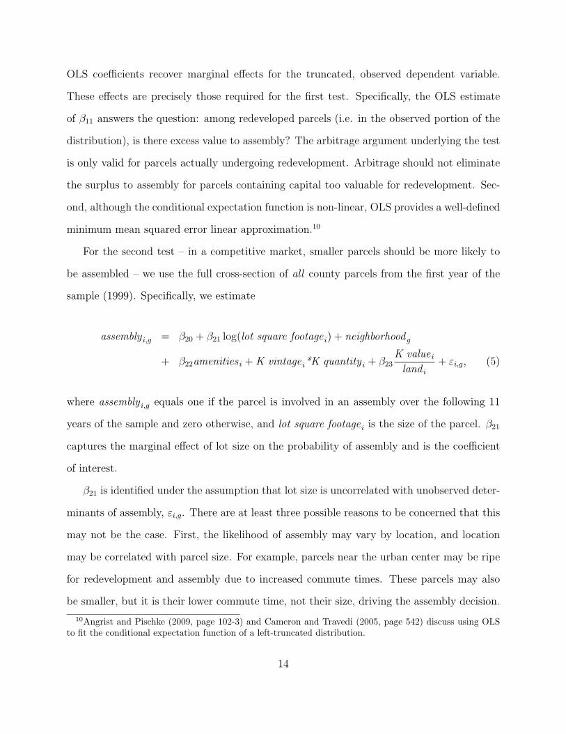
minimum mean squared error linear approximation.10
For the second test – in a competitive market, smaller parcels should be more likely to
be assembled – we use the full cross-section of all county parcels from the first year of the
+ β22amenities i + K vintage i*K quantity i + β23K value i
land i
+ εi,g, (5)
where assembly i,g equals one if the parcel is involved in an assembly over the following 11
years of the sample and zero otherwise, and lot square footage i is the size of the parcel. β21
captures the marginal effect of lot size on the probability of assembly and is the coefficient
of interest.
β21 is identified under the assumption that lot size is uncorrelated with unobserved deter-
minants of assembly, εi,g. There are at least three possible reasons to be concerned that this
may not be the case. First, the likelihood of assembly may vary by location, and location
may be correlated with parcel size. For example, parcels near the urban center may be ripe
for redevelopment and assembly due to increased commute times. These parcels may also
be smaller, but it is their lower commute time, not their size, driving the assembly decision.
10Angrist and Pischke (2009, page 102-3) and Cameron and Travedi (2005, page 542) discuss using OLSto fit the conditional expectation function of a left-truncated distribution.
14
As in the first test, we net out such neighborhood-specific factors with tract or block group
fixed effects, so that all our comparisons are made within a given, limited geographic area.
The second threat to the credibility of the identifying assumption is the possibility that
large plots tend to have more valuable capital per square foot of land than smaller parcels. All
else equal, the more valuable the capital on a parcel, the less likely the capital is scrapped to
allow for redevelopment and the less likely is assembly. Larger lots may very well have more
valuable capital. For instance, if small lots tend to contain two-story single family homes,
whereas large lots tend to contain multi-story buildings, larger lots will have systematically
more capital. We therefore control for the presence of capital in a flexible, relatively non-
parametric manner by including a full set of interaction terms between indicator variables
for the vintage of the existing capital, K vintage i, and indicator variables for the size or
quantity of the capital per square foot of land, K quantity i. This approach fails to account
for both differences in depreciation across properties and differences in the initial quality of
the capital given its size. We therefore also control for the ratio of the value of improvements
(i.e. capital) to the value of land, K value i
land i. Unfortunately, as discussed below, this variable
suffers from measurement error concerns.
A third reason lot size may be correlated with the error term is because not all lots are
“assemble-able,” and “assemble-ability” may be correlated with lot size. To be assembled, a
parcel needs a contiguous neighbor, one not separated by an existing road or other physical
barrier. The most extreme example of an “un-assemble-able” parcel would be one that takes
up an entire city block. Such a parcel cannot be assembled given the existing structure of
roads. In general, larger parcels should be more likely to be unable to assemble for such
reasons. However, this possibility will tend to bias our estimation toward failing to reject
the hypothesis that smaller parcels are more likely to be assembled (and hence make it less
likely we will conclude the market for assembly is inefficient).
We implement the third test – in an efficient market, small parcels should not sell into
15
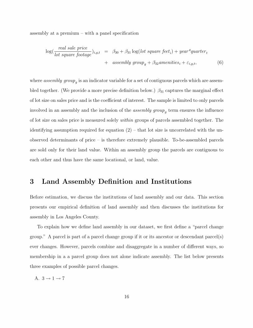
assembly at a premium – with a panel specification
log(real sale price
lot square footage)i,g,t = β30 + β31 log(lot square feet i) + year*quarter t
+ assembly groupg + β32amenities i + εi,g,t, (6)
where assembly groupg is an indicator variable for a set of contiguous parcels which are assem-
bled together. (We provide a more precise definition below.) β31 captures the marginal effect
of lot size on sales price and is the coefficient of interest. The sample is limited to only parcels
involved in an assembly and the inclusion of the assembly groupg term ensures the influence
of lot size on sales price is measured solely within groups of parcels assembled together. The
identifying assumption required for equation (2) – that lot size is uncorrelated with the un-
observed determinants of price – is therefore extremely plausible. To-be-assembled parcels
are sold only for their land value. Within an assembly group the parcels are contiguous to
each other and thus have the same locational, or land, value.
3 Land Assembly Definition and Institutions
Before estimation, we discuss the institutions of land assembly and our data. This section
presents our empirical definition of land assembly and then discusses the institutions for
assembly in Los Angeles County.
To explain how we define land assembly in our dataset, we first define a “parcel change
group.” A parcel is part of a parcel change group if it or its ancestor or descendant parcel(s)
ever changes. However, parcels combine and disaggregate in a number of different ways, so
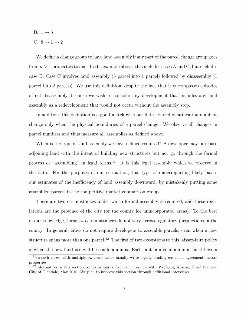
membership in a a parcel group does not alone indicate assembly. The list below presents
three examples of possible parcel changes.
A. 3 → 1 → 7
16
B. 1 → 5
C. 8 → 1 → 2
We define a change group to have land assembly if any part of the parcel change group goes
from n > 1 properties to one. In the example above, this includes cases A and C, but excludes
case B. Case C involves land assembly (8 parcel into 1 parcel) followed by disassembly (1
parcel into 2 parcels). We use this definition, despite the fact that it encompasses episodes
of net disassembly, because we wish to consider any development that includes any land
assembly as a redevelopment that would not occur without the assembly step.
In addition, this definition is a good match with our data. Parcel identification numbers
change only when the physical boundaries of a parcel change. We observe all changes in
parcel numbers and thus measure all assemblies as defined above.
When is the type of land assembly we have defined required? A developer may purchase
adjoining land with the intent of building new structures but not go through the formal
process of “assembling” in legal terms.11 It is this legal assembly which we observe in
the data. For the purposes of our estimation, this type of underreporting likely biases
our estimates of the inefficiency of land assembly downward, by mistakenly putting some
assembled parcels in the competitive market comparison group.
There are two circumstances under which formal assembly is required, and these regu-
lations are the province of the city (or the county for unincorporated areas). To the best
of our knowledge, these two circumstances do not vary across regulatory jurisdictions in the
county. In general, cities do not require developers to assemble parcels, even when a new
structure spans more than one parcel.12 The first of two exceptions to this laissez-faire policy
is when the new land use will be condominiums. Each unit in a condominium must have a
11In such cases, with multiple owners, owners usually write legally binding easement agreements acrossproperties.
12Information in this section comes primarily from an interview with Wolfgang Krause, Chief Planner,City of Glendale, May 2010. We plan to improve this section through additional interviews.
17
separate parcel, as each unit may have a unique legal owner. Therefore, any land combined
for condos must be assembled.
The second exception from the laissez-faire policy is a function of the use of the property.
Suppose that a city’s zoning requires two parking spaces for each multi-family unit, and that
the developer has purchased two parcels upon which to build a new multi-family development.
If the developer builds the parking on one parcel and the structure on the other, he is required
to legally assemble the parcels. Cities make such a requirement to ensure that all future sales
keep parcels in compliance with zoning regulations. The developer can avoid the requirement
to legally assemble by building a structure that spans both parcels.
Even if it is not legally required, a developer may still wish to assemble parcels. Selling
an assembled parcel, rather than multiple unassembled parcels reduces uncertainty in future
transactions. Assembly also yields a reduction in legal paperwork.
It is important to note that the legal land assembly process does not trigger a reassessment
under California’s Proposition 13. Proposition 13 limits the increase of a property’s assessed
value to two percent per year, and the assessed value raises to market value at sale. Thus,
a developer may face a increase assessment due to property purchase, but does not face an
increased assessment due to the legal act of assembly.13
4 Data
Our project relies on multiple sources of data. We summarize the data here, and refer
interested readers to our lengthy Data Appendix for full details on all data inputs and data
construction details. The three key components of our data are the annual property-level
data for Los Angeles County, sales data for properties, and census neighborhood measures.
Our annual property data consist of three key parts: (i) ten annual cross-sectional obser-
13This information comes from the Special Investigations Section, Los Angeles County Assessor.
18
vations of the 2.2 million parcels in the County of Los Angeles, (ii) a dataset listing all parcels
that change, and the number of the parcel(s) to which they change, and (iii) electronic maps
with geographic information on all properties.
The annual cross-sections are the heart of the dataset. In each year from 1999 to 2010
(except for 200314) we observe attributes about each individual piece of property in the
88 cities and the large unincorporated area of Los Angeles County. We observe too many
attributes to list here, but briefly the data include attributes about the property itself (e.g.,
size and location); attributes about the building on the property (e.g., building size); and
attributes about the legal regime that governs the property (i.e., the use and zoning rules
for each property). Thus, this part of the dataset includes somewhat more than 24 million
observations with many descriptive variables.
The second part of the data is a file that allows us to take the 11 cross-sections and make
them into a true panel by linking property identification numbers over time. Though most
properties retain a constant identification number throughout the sample, some properties
split or merge. Our dataset of all property identification number changes allows us to follow
each initial piece of land to its current, perhaps aggregated or disaggregated, form. While
this task is conceptually simple, it has mechanically been quite difficult, and the bulk of our
data assembly has been devoted to making sure that we have built these linkages correctly.
The third and final part of the annual property data is electronic maps of all parcels.
These maps, which we have from 2006 onward, allow us to pinpoint the exact location of
each individual property and calculate distances from one property to another, or from a
given property to key urban amenities, such as light rail stops or freeways. These maps also
allow us to assign each property to an unique census block group.15
We combine this panel of all properties in the county with all property transactions by
14We were never able to get access to this cross-section.15On average, populated block groups in Los Angeles contain approximately 1,400 people.
19
property identifier. Specifically, we observe the last three sales on each property as of 2006,
and sales in the last two years from 2009 and 2010. This leaves a small gap of sales in 2006.
We limit the sample of transactions to include only arms’ length transactions and make other
small adjustments as defined in the Data Appendix.
We measure neighborhood economic and demographic factors with data from the 1990
and 2000 Decennial Censuses at the block group level. To use the 1990 block group data,
we use GIS mapping to make a correspondence from 1990 to 2000 census block groups.
5 Results
We now turn to describing the results of each our three tests in turn.
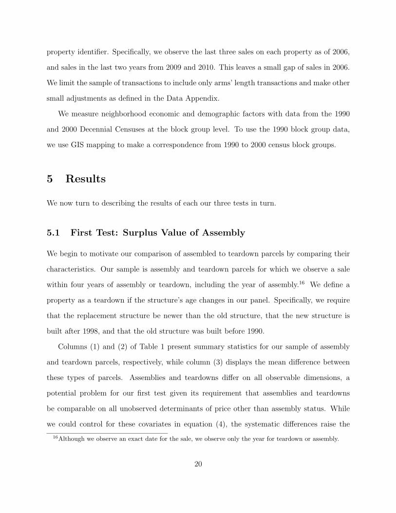
5.1 First Test: Surplus Value of Assembly
We begin to motivate our comparison of assembled to teardown parcels by comparing their
characteristics. Our sample is assembly and teardown parcels for which we observe a sale
within four years of assembly or teardown, including the year of assembly.16 We define a
property as a teardown if the structure’s age changes in our panel. Specifically, we require
that the replacement structure be newer than the old structure, that the new structure is
built after 1998, and that the old structure was built before 1990.
Columns (1) and (2) of Table 1 present summary statistics for our sample of assembly
and teardown parcels, respectively, while column (3) displays the mean difference between
these types of parcels. Assemblies and teardowns differ on all observable dimensions, a
potential problem for our first test given its requirement that assemblies and teardowns
be comparable on all unobserved determinants of price other than assembly status. While
we could control for these covariates in equation (4), the systematic differences raise the
16Although we observe an exact date for the sale, we observe only the year for teardown or assembly.
20
possibility that assembly and teardown parcels differ on unobserved dimensions.
Column (4), however, presents regression-adjusted mean differences conditioned on census
tract fixed effects.17 In this and all following regressions, we report standard errors clustered
at the tract level. With the comparison between the two parcel types made only within
small neighborhoods, differences are very small and imprecise. The notable exception is the
probability of being a single family parcel. Overall, we view the results of column (4) as
supportive of our identification strategy which relies on geographic fixed effects to control
for unobservable differences between the two types of parcels. The right half of the table
repeats this exercise for neighborhood demographic variables which are expressed as the level
difference between 1990 and 2000 values. The same pattern of no difference conditional on
tract-level fixed effects holds.
Given the results in Table 1, we take care below to address the difference in single family
status. Most specifications include a control for use type. We also present specifications
that restrict the sample to only single family parcels or non-residential parcels to make the
teardowns and assemblies as comparable as possible.
Table (2) presents the results for our first test (in a competitive equilibrium, the price of
teardowns and assembly parels should equate), implemented by estimating equation (4) on
the panel of teardowns and assemblies. The coefficient estimate in column (1) indicates that
being in an assembly is associated with an almost 65 percent sales price premium relative
to being sold for redevelopment without a change in parcel boundaries. The extremely large
magnitude of the assembly surplus suggests substantial frictions in the market for assembly.
Columns (2) - (4) present alternative specifications. Column (2) addresses within neigh-
borhood variation by adding neighborhood demographic controls at the block group level
and controls for local amenities. Column (3) further addresses intra-neighborhood variation
17The demographic characteristics, such as the poverty rate, are from the census and are measured at theblock group level. The census tracts in the sample on Table 1 have an average of 2.5 block groups withinthem.
21
by controlling for very finely grained neighborhood effects. Instead of tract fixed effects,
we use block group fixed effects. Column (4) controls for the evolution in price specific
to each tract by using tract fixed effects and tract-level linear trend terms. Regardless of
specification, the magnitude of the surplus estimate falls only slightly.
The remaining columns use different subsets of the sample. Column (5) includes assem-
blies only if we observe that the existing capital is torn down and replaced with new capital
following assembly. It is possible that assemblies may occur with the aim of redeveloping
at some point in the future, not immediately. If so, the sales price of the to-be-assembled
parcels reflects the return to any existing capital over the period before redevelopment. Such
a scenario would bias our surplus estimates upward. In this case, estimates in Columns (1)
to (4) should be interpreted as upper bounds.
However, we can identify assemblies that lead to immediate new construction. Due to
the nature of our data, we under-identify these parcels. For a given assembly, pre-assembly,
we observe attributes for one structure per parcel, though a parcel may, in fact, contain more
than one parcel. For each parcel change group before assembly, we find the minimum and
maximum of the age of the structure on each parcel: max(agec,before) and min(agec,before) (c
indicates a parcel change group). We observe similar ages post-assembly: max(agec,after) and
min(agec,,after). We define parcels as being assembly teardowns only if max(agec,before) <
min(agec,after). This is likely too restrictive, so we interpret results from this sample as lower
bound estimates of the surplus. Though these results are smaller, the magnitude is similar
to the unrestricted sample.
To address the concern that assembled parcels are systematically less likely to be single
family than are teardowns, Columns (6) and (7) restrict the sample to single family parcels
only. The results increase in magnitude somewhat. Columns (8) and (9) restrict the sample
to non-residential properties only and report estimates similar to that produced by the full
sample.
22
5.2 Second Test: The Influence of Lot Size on the Probability of
Assembly
Our second test states that in an efficient market, developers should prefer to assemble larger
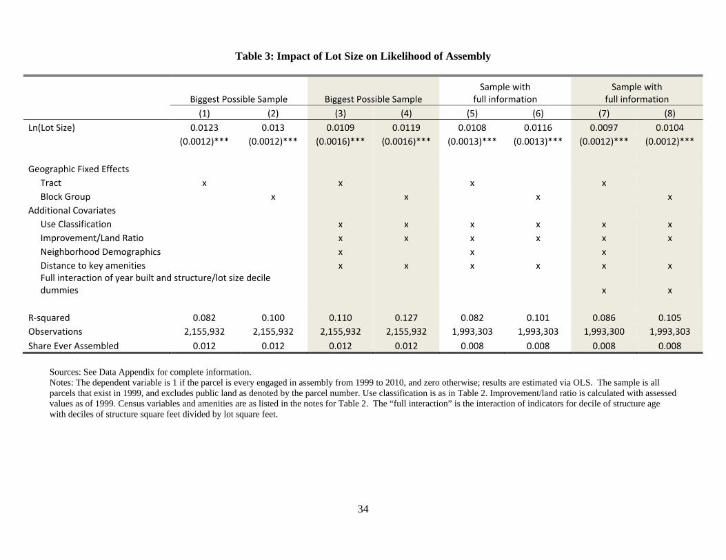
parcels. Table 3 presents the results for this second test, implemented by estimating equation
(5) on the 1999 cross-section of all parcels.18 The coefficient in column (1) indicates that a
10 percent increase in the size of a parcel increases the probability of ever being assembled
by 0.1 percent. This is a large effect, equal to 10 percent of the sample mean probability of
ever assembling (see the bottom row of the table). The estimate can also be interpreted as
indicating that the elasticity of the probability of assembly with respect to lot size is roughly
1.
Columns (2) - (4) present specification permutations which result in very little change
in the lot size coefficient. In column (2), the estimates are robust to conditioning on the
extremely finely grained block group fixed-effect. To better purge intra-neighborhood varia-
tion, Columns (3) and (4) add parcel- and neighborhood-specific covariates. Parcel-specific
covariates are dummies for use type (four categories), the improvement to land ratio (from
1999 reported assessed values for each) and the distance to key amenities as above. The im-
provement to land ratio is measured with error, as Proposition 13 caps increases in assessed
values to 2 percent per year until sale. Neighborhood demographics are as in the first test.
As neighborhood demographics are observed at the block group level, we omit them in all
specifications with block group fixed effects.
Across specifications, and despite the fact that the model argues that the surplus to
assembly is largest for small parcels, large parcels are more likely to assemble. Thus, this
evidence is consistent with the theory that holdouts and strategic delay impede the market
for assembly.
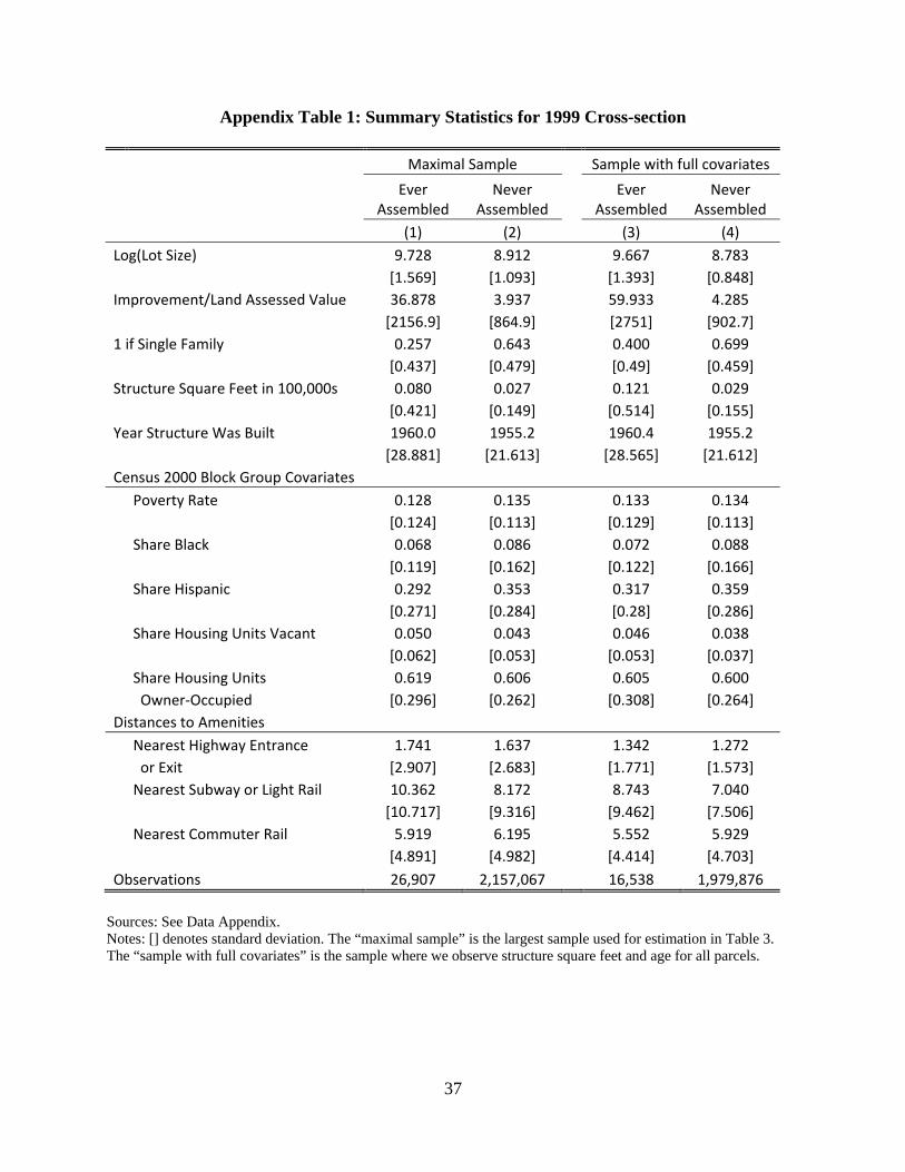
18Summary statistics for this sample are in Appendix Table 1.
23
The K vintage i ∗K quantity i terms (full interactions of decile dummies for structure size
per lot square foot and structure age) are not included in columns (1) - (4). We are interested
in results conditional on these variables, because they are a relatively non-parametric method
of capturing the quantity and quality of capital per parcel. Including these terms, which
are not available for all parcels, truncates the sample. For comparison purposes, columns
(5) and (6) replicate columns (3) and (4) using the truncated sample without adding the
K vintage i ∗ K quantity i terms. Although around one-third of the assemblies are lost from
the sample – see the bottom row – the lot size coefficient is essentially unchanged. Columns
(7) and (8) add in the K vintage i∗K quantity i terms and again the coefficient is little altered.
Table 4 presents robustness checks based on columns (7) and (8) of Table 3. To examine
whether effects differ by initial use, consistent with the concern raised in Table 1, columns
(1) and (2) restrict the sample to only single family parcels, while columns (3) and (4)
restrict the sample to only non-residential parcels. The marginal effect of lot size on the
likelihood of assembly is remarkable consistent across these use categories. The remaining
columns exclude the least dense block groups in order to ensure our results are driven by
outcomes in a dense urban setting. The parcels excluded are generally located in outlying
areas of the county where land subdivision and new development, as opposed to assembly
and redevelopment, are likely more prevalent. Again, the results are little changed.
5.3 Third Test: Influence of Lot Size on Price of To-Be-Assembled
Parcels
Given our finding that the amount of land assembly is inefficiently low, we now move to
our third test: in an efficient equilibrium, small parcels should not sell into assembly at
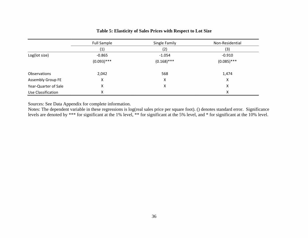
a premium. Table 5 presents the results for this third test, implemented by estimating
equation (6) on the panel of parcels ever involved in an assembly and for which we observe a
24
sale either in the year of or in the three years prior to the assembly. Column (1) includes all
use types, while columns (2) and (3) restrict the sample to single family and non-residential.
The results indicate that a 10 percent increase in parcel size reduces the sales price of a
to-be-assembled parcel by roughly 9 to 10 percent. Alternatively, the results suggest an
elasticity of price with respect to lot size of around 1. The substantial premium to small
parcels supports the hypothesis that owners of small parcels of land tend to hold out and
demand higher than average prices for their land – behavior which works to reduce the
number of successful assemblies.
6 Conclusion
In sum, the evidence offers a robust rejection of the conjecture that the market for land
assembly functions efficiently. This rejection occurs despite the fact that land ownership is
clearly defined, a precondition for an efficient transaction. Our evidence on the premium
paid to small parcels suggests that at least part of this inefficiency is due to private market
failures, and not to governmental regulation of land. These findings speak to the workings
of land value taxation, the literature on the regulatory tax, and the historiography of urban
renewal.
Rejecting the efficiency of land assembly means that the price of land sold for assembly is
not the “true” competitive market price. This calls into question the literal base of land value
taxation. Within a jurisdiction, this excess price for assembled land means that assembled
land pays a larger share of the jurisdiction’s tax revenue, further lowering the likelihood of
land assembly. The excess price also means that the efficiency of land value taxation is also
called into question.
Glaeser and Gyourko (2002) and Glaeser et al. (2005), and a following literature, defines
the regulatory tax as the difference between the competitive market price for land and
25
the observed price for land. It then attributes this difference to market failures due to
government regulation. This paper points out that the wedge between the competitive and
observed prices contains – at least in the case of parcels purchased for assembly, which we
know to be a non-trivial amount of new construction – the effects of both public and private
market failures. Thus, this methodology may overstate the impact of the regulatory tax. In
future work, we hope to examine the role of public market constraints on the likelihood of
assembly.
If land assembly indeed operates as inefficiently as we suggest in this work, it is natural
to look to government for remediation. The most recent large-scale government action to
assemble land is what is known as “urban renewal,” a process in the United States, Canada
and in some parts of Europe in the 1960s and 70s. Urban renewal used the government’s
power of eminent domain to assemble small parcels of land, predominantly in the urban
core. While readers may associate renewal with tall towers of public housing, this was
not its predominant output. Urban renewal generated substantial high and middle income
housing, as well as non-residential construction. Copley Place in Boston, and the “new
downtown” atop Bunker Hill in Los Angeles are both examples of urban renewal. Urban
renewal ended amid charges of developer cronyism and racism, and has largely been judged
harshly by historians (Cord, 1974). Our results suggest that urban renewal may have been
a bad but best solution to a very difficult problem.
26
References
Angrist, Joshua and Pischke, Jorn-Steffen, 2009. Mostly Harmless Econometrics: An Em-piricist’s Companion. Princeton: Princeton University Press.
Asami, Y., 1988. “A game-theoretic approach to the division of profits from economic landdevelopment.” Regional Science and Urban Economics 18: 233–246.
Bogart, Dan and Richardson, Gary, 2009. “Making property productive: reorganizing rightsto real and equitable estates in Britain, 1660-1830.” European Review of Economic History13: 3–30.
Brownstone, David and DeVany, Arthur, 1991. “Zoning, Returns to Scale, and the Value ofUndeveloped Land.” Review of Economics and Statistics 73(4): 699–704.
Cadigan, John, Schmitt, Pamela, Shupp, Robert, and Swope, Kurtis, 2010. “The HoldoutProblem and Urban Sprawl: Experimental Evidence.”
Cameron, A. Colin and Travedi, Pravin K., 2005. Microeconometrics: Methods and Appli-cations. Cambridge: Cambridge University Press.
Colwell, Peter and Sirmans, C. F., 1993. “A Comment on Zoning, Returns to Scale and theValue of Undeveloped Land.” Review of Economics and Statistics 75(4): 783–786.
Colwell, Peter F. and Munneke, Henry J., 1997. “The structure of urban land prices.”Journal of Urban Economics 14: 321–336.
Colwell, Peter F. and Munneke, Henry J., 1999. “Land Prices and Land Assembly in theCBD.” Journal of Real Estate Finance and Economics 18(2): 163–180.
Cord, Steven, 1974. “Urban Renewal: Boon or Boondoggle?” American Journal of Eco-nomics and Sociology 33(2): 184–186.
Cunningham, Christopher, 2010. “Estimating the holdout problem in land assembly.” Fed-eral Reserve Bank of Atlanta Working Paper.
Dye, Richard F. and McMillen, Daniel P., 2007. “Teardowns and land values in the Chicagometropolitan area.” Journal of Urban Economics 61: 45–63.
Eckart, Wolfgang, 1985. “On The land assembly problem.” Journal of Urban Economics 18:364–378.
Field, Alexander James, 1992. “Uncontrolled Land Development and the duration of theDepression in the United States.” Journal of Economic History 52(4): 785–805.
Fu, Daniel P. McMillen, Yuming and Somerville, Tsur, 2002. “Land Assembly: MeasuringHoldup.” University of British Columbia Centre for Urban Economics Working Paper02-08.
27
Glaeser, Edward and Gyourko, Joseph, 2002. “The Impact of Zoning on Housing Afford-ability.” NBER Working Paper No. 8835.
Glaeser, Edward, Gyourko, Joseph, and Saks, Raven, 2005. “Why is Manhattan so Expen-sive? Regulation and the Rise in Housing Prices.” Journal of Law and Economics XLVIII:331–369.
Grossman, Zachary, Pincus, Jonathan, and Shapiro, Perry, 2010. “A Second-Best Mechanismfor Land Assembly.”
Harding, John P., Rosenthal, Stuart, and Sirmans, C. F., 2003. “Estimating BargainingPower in the Market for Existing Homes.” Review of Economics and Statistics 85(1):178–188.
Henderson, J. Vernon, 1977. Economic Theory and the Cities. New York: Academic Press.
Jacobs, Jane, 1961. The Death and Life of Great American Cities. New York: VintageBooks.
Libecap, Gary D., Lueck, Dean, and O’Grady, Trevor, 2010. “Large Scale InstitutionalChanges: Land Demarcation Within the British Empire.” NBER Working Paper No.15820.
Menezes, Flavio and Pitchford, Rohan, 2004. “The land assembly problem revisited.” Re-gional Science and Urban Economics 34: 155–162.
Miceli, Thomas and Segerson, Kathleen, 2007. “A bargaining model of holdouts and takings.”American Law and Economics Review 9(1): 160–174.
Miceli, Thomas J and Sirmans, C. F., 2007. “The holdout problem, urban sprawl, andeminent Domain.” Journal of Housing Economics 16: 209–219.
Munch, Patricia, 1976. “An Economic Analysis of Eminent Domain.” Journal of PoliticalEconomy 84(3): 473–497.
Nelson, Arthur and Lang, Robert, 2007. “The Next 100 million.” Planning 73(1): 4–6.
Rosenthal, Jean-Laurent, 1990. “The Development of Irrigation in Provence, 1700-1860: TheFrench Revolution and Economic Growth.” Journal of Economic History 50(3): 615–638.
Rosenthal, Stuart and Helsley, Robert W., 1994. “Redevelopment and the Urban Land PriceGradient.” Journal of Urban Economics 35: 182–200.
Shoup, Donald, 2008. “Graduated Density Zoning.” Journal of Planning Education andResearch 28(2): 161–179.
Strange, William C., 1995. “Information, Holdouts and Land Assembly.” Journal of UrbanEconomics 38: 317–332.
29
30
Figure 1: Ratio of Assemblies to Permits
Sources: Permit data from Census Bureau, assemblies calculated from authors’ dataset. See Data Appendix for details. Notes: While the Census Bureau counts one permit for each new unit, one assembly (in our terms) may result in more than one unit. This means that our measure in the chart understates the importance of assembly. However, the Census Bureau counts residential permits only, while our measure of assemblies includes assemblies that result in non-residential construction. This leads to this measure overstating the importance of assembly. Because we do not have a cross-section of properties from 2003, we all assemblies in 2002 and 2003 are attributed to 2002; for the purposes of this chart, we split the assemblies in 2002 evenly between 2002 and 2003. Though our assembly information continues through 2010, this chart ends in 2008 when our permit data ends.
31
Figure 2: Price Per Square Foot is Convex in Lot Size
Notes: This picture shows that the price per square foot of land increases with lot size at an increasing rate.
32
Table 1: Summary Statistics for Price Analysis
Levels Change from 1990 to 2000
Assembled Teardown Difference Difference conditional on tract FE
Assembled Teardown Difference Difference conditional on tract FE
Sources: See Data Appendix for complete information. Notes: Columns (1), (2), (5) and (6) present means. Columns (3) and (7) present equality of means test for the means presented in columns (1) and (2), and (5) and (6), respectively. Columns (4) and (8) present coefficient estimates from a regression of the variable in the row on an indicator variable for assembly and a set of census tract fixed-effects. [] denotes standard deviation and () denotes standard error. Significance levels are denoted by *** for significant at the 1% level, ** for significant at the 5% level, and * for significant at the 10% level.
33
Table 2: Excess Value of Land in Assembly
Full Sample Single Family Non‐Residential
(1) (2) (3) (4) (5) (6) (7) (8) (9) 1 if Parcel is in an assembly 0.638 0.550 0.532 0.534 0.484 0.782 0.808 0.581 0.501
Geographic Fixed Effects Tract X X X X X X X X Block Group X Additional Covariates Year‐Quarter of Sale X X X X X X X X X Use Classifications X X X X X X X X X Cubic in Lot Size X X X X X X X X X Neighborhood Demographics X X X X Distance to Key Amenities X X X X Linear Tract Trends X
Assembly Teardowns X
Sources: See Data Appendix for complete information. Notes: The dependent variable in these regressions is log(real sales price per square foot). () denotes standard error. Significance levels are denoted by *** for significant at the 1% level, ** for significant at the 5% level, and * for significant at the 10% level. Neighborhood demographics, obtained from the census, include the following variables in both 2000 level form and as changes between 1990 and 2000 levels: poverty rate, neighborhood share black, neighborhood share hispanic, share of housing units vacant and share of housing units owner-occupied. Use classifications include indicator variables for: single family, non-condo multi-family, condo, vacant and other. Distance to key amenities include measures for the shortest distance from each parcel to three amenities: a highway entrance or exit, a metrolink stop (commuter rail), and a metrorail stop (subway or light rail).
34
Table 3: Impact of Lot Size on Likelihood of Assembly
Biggest Possible Sample Biggest Possible Sample Sample with
Additional Covariates Use Classification x x x x x x Improvement/Land Ratio x x x x x x Neighborhood Demographics x x x Distance to key amenities x x x x x x Full interaction of year built and structure/lot size decile dummies x x
Sources: See Data Appendix for complete information. Notes: The dependent variable is 1 if the parcel is every engaged in assembly from 1999 to 2010, and zero otherwise; results are estimated via OLS. The sample is all parcels that exist in 1999, and excludes public land as denoted by the parcel number. Use classification is as in Table 2. Improvement/land ratio is calculated with assessed values as of 1999. Census variables and amenities are as listed in the notes for Table 2. The “full interaction” is the interaction of indicators for decile of structure age with deciles of structure square feet divided by lot square feet.
35
Table 4: Robustness Results for Impact of Lot Size on Likelihood of Assembly
By Use Type Parcel is in a Block Group with Density is Greater Than
Single‐Family Residential Only Non‐Residential Only
Additional Covariates x x x x x x x x R‐squared 0.057 0.078 0.203 0.265 0.086 0.105 0.079 0.093 Observations 1,389,272 1,389,272 148,411 148,414 1,993,300 1,993,303 1,759,088 1,759,091
Sources: See Data Appendix for complete information. Notes: The dependent variable is 1 if the parcel is every engaged in assembly from 1999 to 2010, and zero otherwise; results are estimated via OLS. The sample is all parcels that exist in 1999, and excludes public land as denoted by the parcel number. All covariates are as in final column of the previous table. Results estimated when using the biggest possible sample and omitting controls for structure year built and structure square feet per lot square feet are very similar.
36
Table 5: Elasticity of Sales Prices with Respect to Lot Size
Full Sample Single Family Non‐Residential
(1) (2) (3) Log(lot size) ‐0.865 ‐1.054 ‐0.910
(0.093)*** (0.168)*** (0.085)***
Observations 2,042 568 1,474 Assembly Group FE X X X
Year‐Quarter of Sale X X X
Use Classification X X
Sources: See Data Appendix for complete information. Notes: The dependent variable in these regressions is log(real sales price per square foot). () denotes standard error. Significance levels are denoted by *** for significant at the 1% level, ** for significant at the 5% level, and * for significant at the 10% level.
37
Appendix Table 1: Summary Statistics for 1999 Cross-section
Sources: See Data Appendix. Notes: [] denotes standard deviation. The “maximal sample” is the largest sample used for estimation in Table 3. The “sample with full covariates” is the sample where we observe structure square feet and age for all parcels.
Data Appendix
This appendix describes how we created the Los Angeles County parcel dataset. Section
1 describes the input datasets. Section 2 describes how we join these datasets, and reports
statistics on the uncleaned data. Section 3 describes how we clean the joined dataset, and
Section 4 reports statistics on the quality of the final dataset.
1 Data Sources
The basic unit of analysis is the parcel, which is an individual property as legally defined by
the Los Angeles County Assessor and Recorder. In any year, there are roughly 2.3 million
parcels in the County of Los Angeles. We rely on a number of different sources for information
about parcels.
1.1 Parcel-Level Data
For detailed property information on parcels, we rely on data from three separate vendors:
DataQuick, Applied Geodetics, and the Los Angeles County Assessor directly.
1.1.1 DataQuick: 1999 - 2002
Dataquick is a property information vendor. It purchases property information from the Los
Angeles County Assessor to sell to real estate professionals. We rely on Dataquick data for
1999-2002, and data are reported as of January of each year.
As far as we can ascertain, the Dataquick data are a slightly modified version of the
“Secured Basic File” that the Assessor prepares. Dataquick modifies the data from the
original Los Angeles County format, and we re-modify it to be consistent with the two
following datasets. We discuss modifications at length in Section 3. This data vendor is
abbreviated in tables as DQ.
1
1.1.2 Applied Geodetics: 2004 - 2006
Applied Geodetics is a mapping firm in Los Angeles County. Applied Geodetics sold us
data for 2004 (April), 2004 (February) and 2005 (May). To the best of our knowledge,
these data are the unmodified Assessor’s “Secured Basic File,” which is the most complete
record of property attributes available to the public from the Assessor. This data vendor is
abbreviated in tables as AG.
1.1.3 Los Angeles County Assessor, Local Roll: 2007 - 2009
From 2007 through 2009, we have purchased data directly from the Assessor. Due to financial
constraints we purchased the “Local Roll” database (roughly $400) instead of the “Secured
Basic File” (roughly $13,000). The Local Roll has fewer parcel attributes than the Secured
Basic File, and comes out annually in July. This data source is abbreviated in tables as LR.
1.1.4 Los Angeles County Assessor, Secured Basic File: 2010
In 2010, we purchased the Secured Basic File, which is the County’s most complete publicly
available dataset about properties. These data are from July 2010, and this data source is
abbreviated in tables as SB.
1.2 Sales Data
1.2.1 Last Three Sales, 1980 to 2006
In 2006, Brooks purchased a file from the County Assessor that contains information on the
last three transactions for each property in the county. For each transaction, we observe
transaction type, sale amount (if applicable), and date of transaction.
2
1.2.2 Sales Within Two Years: 2008, 2009, and 2010 Files
In 2008, 2009, and 2010, we purchased additional lists of sales data from the County Assessor.
These contain information on all transactions in the prior two years. For each transaction,
we observe transaction type, sale amount (if applicable), and date of transaction.
These files leave a small gap from May through December 2006 which we have not been
able to obtain.
1.3 Parcel Change Database
At our request, the Assessor made a special file that includes all parcel changes from July
1999 January 2009. Specifically, for each change, this file includes the old parcel number(s),
the new parcel number(s), and the effective date of the change. The County has electronic
records for parcel changes starting in July 1999 and continuing to the end of our data.
This change database allows us to isolate land assembly and disassembly. The California
Assessor’s Handbook mentions only one reason for a parcel number to change: if the physical
boundaries of a parcel are modified (California State Board of Equalization, 1997, page 26).
We purchased this change database again in July 2009 and 2010 (covering all changes in
the past two years) to allow us to link all later parcels with previous parcels.
1.4 Digital Parcel Maps
For each year since 2006, we have an electronic map of all parcels that exist in that year.
These maps have a boundary (a polygon) for each individual parcel. For each parcel, we
use ArcGIS to calculate the x- and y-coordinates (latitude and longitude) of the polygon’s
geographic center (centroid).
3
1.5 Census Tract and Block Group Indentification
The Census provides census tract and block group boundaries in shapefile format online.1
We use ArcGIS to intersect the 2000 census boundaries and the 2006 parcel boundaries to
assign each parcel to a census block group.
The majority – 96% – of ever-existing parcels have block group identifiers.
1.6 Block Group Data
We use block group level data from the 2000 Decennial Census (ICPSR file 13346, summary
level 150), and from the 1990 Decennial Census (ICPSR 9782, summary level 150, but
California file is damaged so we used a similar file downloaded from UCLA ATS).
We use ArcGIS and the Census’s electronic maps to make a linkage between 1990 and
2000-based block groups, where relationships are based on land area overlap.
1.7 Assorted Non-Parcel Digital Maps
• Parks: Information from 2008 ESRI files of local and national parks for California
– parks displayed on maps are only those more than 1.25 square miles
• Freeways: Data from State of California Cal-Atlas Geospatial Clearinghouse
– website is http://www.atlas.ca.gov/download.html
– transportation → Census 2000 → state highways.* and us highways.*
• Freeway Entrances and Exits
– Tele-Atlas US Data, contains federal interstate highway entrances and exits
• Coastline
– layer of points every 1000 feet along LA County coastline
– created by taking Census 2000 county map and deleting non-coastline portions
– used X-tools feature to points to convert coastline line to points
1Files are at http://www.census.gov/geo/www/cob/bdy files.html.
4
• Metrolink Stations
– Commuter rail stations
– File received from Javier Minjares, Southern California Association of Govern-ments, 2010
• Metro Rail Stations
– Intra-urban rail stations
– File received from Javier Minjares, Southern California Association of Govern-ments, 2010
• Major Roads
– Tele-Atlas US Data, version 9.3
– Major roads only
2 Initial Data Linking
Each parcel is identified by a 10-digit number: MMMM-PPP-XXX. The first four digits are
the “map book” number – literally the number of the “book” in which the parcel appears.
The second three digits are the map book page. Each map book page contains a set of
geographically contigious parcels. The last three digits identify individual parcels on the
map book page.
We began the data assembly by attempting to link all the annual cross-sections described
above (1999-2009, without the missing 2003) using the parcel change database. Panel A of
Table 1 presents the results of this original linkage. Slightly fewer than 2 million parcels never
change their number throughout the sample (column 2). Column 3 reports the number of
ever-changing parcels; this number varies by year as a changer could be 3 parcels in 1999,
but 12 (or 1) parcels in 2009. The number of changes in any given year varies from 28,996
to 58,557. Column 4 reports the number of parcels that exist in this year of the sample,
but not in all years of the sample. Column 4 shows a striking number of parcels that exist
5
after 2004, but not before. These missing, or “phantom,” observations are due to DataQuick
editing. We discuss how we deal with these discrepancies in the next section.
We also analyze the total amount of land area, measured in square feet, in each category
as a check on our data assembly process. We report annual totals in Panel B of Table 1.
Columns 2 through 4 report the total amount of parcel square footage in each of the parcel
assembly categories by year. Sadly, for 2004 and 2005 we do not observe parcel size in the
data. It is very clear that across all categories, but particularly in the “phantom” category,
that the total land area is drastically smaller in the earlier data source (DataQuick). The
California Department of Water Resources measures the total land area of Los Angeles
County as 132,487,077,888 square feet, which is clearly much closer to the later data source
(143 billion square feet) than the earlier one (22 billion square feet).2
Table 2 shows the total number of parcels (Panel A) and total land area (Panel B) by
four categories of use types and by year. The Assessor assigns each property a “use code”
that describes how the property is currently used (as distinct from how it is zoned). We
use this code to make four major categories of use: single-family, multi-family, vacant, and
other. The number of vacant parcels by year (column 4) shows a large break concomitant
with the break in data sources, and similar to the break for the “phantom” parcels of the
previous table.3 The bottom panel of the table shows that this discrepancy appears across
types.
3 Cleaning and Consistency Changes
This section details the work we did to make the property data consistent across data sources
and time. The main issues in cleaning the data were how to give a measure of land area to
2Parcels cover all land and water area of the county with the exception of public roadways. We discusslater how the latter datasets “overcount” the county’s land area.
3Vacant parcels may be coded vacant residential, vacant commercial, or simply vacant. “Vacant” appearsto refer to habitation or use, and not to the presence of structures.
6
parcels in 2004 and 2005, how to count the land area of parcels that were vertically stacked,
how to account for parcels present in later years and missing in the earlier years, how to
account for lack of consistency between the change database and the cross-sectional data,
how to deal with reported changes in lot size for parcels that do not change, how to deal
with consistently reporting land area for parcels that make complicated changes, and how
to impute geographic information for parcels pre-dating our electronic maps.
3.1 Defining the Parcel Group
For ease of analysis, we define a “parcel group” to include all parcels linked by a change.
For example, consider a change where parcels A and B combine to C, parcel C splits to D
and E, and E splits to F and G. All parcels A through G would have one parcel group. We
create a unique identifer for each group.
3.2 No Observation of Land Area in 2004 and 2005
The data source we use for 2004 and 2005 does not contain information on parcel land area.
We assume that all 2004 parcels existing in 2002 have the same land area that they did in
2002, and all 2005 parcels existing in 2006 have the same land area they will have in 2006.
These are very reasonable assumptions, as lot size changes only when parcel number does.
As we describe in greater detail below, we use a variety of methods to evaluate and clean lot
size across time.
If a 2004 or 2005 parcel is also missing lot size information in 2002 or 2006, we take lot
size from the closest year for which it is available.
7
3.3 Vertically Stacked Parcels
The assessor draws the boundary for a piece of land with multiple owners, such as a con-
dominium, so that each owner’s parcel has the land area of the entire lot. This type of
separate ownership of the same piece of land is distinct from joint ownership of a single
property. Condominium-type ownership parcels are “stacked” vertically on the Assessor’s
map, in the same way you would stack checkers. In this case, think of each checker as the
condominium of an individual owner. A 100-unit condominium will consist of 100 parcels,
one for each legally distinct unit of ownership. Stacked parcels are usually, but not always,
condominiums.
In the DataQuick data, the land area of each condominium unit is the land area of the
lot divided by the number of parcels covering that lot. In the remaining datasets, when units
and parcels are co-terminous, each unit is assigned the land area of the entire lot. This leads
to much of the discrepancy in land area between the 1999 to 2002 and 2003 to 2010 periods
in Tables 1 and 2. We correct for this problem by modifying all parcels to have a land area
consistent with the method in the DataQuick data (land area of a parcel = total land area of
parcel / number of parcels occupying that lot). We prefer this method of measuring land area
because the net land area remains unchanged even if one parcel becomes three condos. The
method used in the later datasets suggests that the total land area of the county increases
when condominiums are created.
We identify vertically stacked parcels by calculating the centroid of every parcel on each
map we have (annual maps, 2006-2010). In any given year, all parcels that share the same x-
and y-coordinates are “stacked,” and their land area requires correction. On average, a map-
year has 250,562 unique parcels that are stacked, 14,400 stacks, and a mean of 17 parcels
per stack. Unfortunately, we do not have maps for years before 2006, so this correction is
incomplete for 2004 and 2005. Specifically, we can correct all stacked parcels that exist in
2004 and 2005 and which continue to exist in 2006. We cannot correct stacked parcels that
8
exist in 2004 or 2005 and not in 2006.
3.4 “Phantom” Parcels
The third data challenge we faced was the presence of parcels that did not appear in all
years, and the disappearance of which could not be explained by any observation in the
parcel change database. We call these appearing and disappearing parcels “phantoms.”
Table 1 suggests that the DataQuick data do not include all parcels that exist in the
county. We strongly suspect that, in an effort to satisfy customers primarily interested in
residential (or at least tradeable property) property, DataQuick deletes parcels that will not
be transacted.
Table 3 describes the appearance of phantoms across the years of the dataset. The
horizontal axis has one column for each year of the dataset. The vertical axis has one row
for each year of phantom non-appearance. The (1999,2000) cell says that 516 parcels that
exist in the 1999 dataset do not exist in the 2000 dataset and are not accounted for by any
parcel changes. The diagonal axis is by definition zero, since a parcel cannot be missing
in the year in which it exists. The clear and striking pattern in this table is that the vast
majority of phantom parcels are missing in in the years 1999 to 2002, and come from datasets
in years 2004 to 2010.
To resolve this problem, we say that any parcel that ever exists in the dataset is a “true”
parcel. Because these parcels are not in the change database, we assume that their shape
is constant over the period of interest and that they exist in all years. Roughly 200,000 of
these parcels truly exist from 2004 to 2010 and do not appear from 1999 to 2002. Only
about 20,000 parcels appear from 1999 to 2002 and not from 2004 to 2010. Were we not to
make this adjustment, we would have an severely unbalanced panel, and the early years of
the panel would not account for a substantial amount of the land area of the County.
9
3.5 Relating Parcel Change to Parcel Cross-sectional Databases
We use the assessor’s parcel change database to link parcels across years. The assessor
reports on changes of four types: one to many, one to one, many to one, zero to one and one
to zero. These last two changes (zero to one and one to zero) are the least frequent of all
change types. They are used to move land in and out of the county. Land in use by roads
does not have parcels, so the addition of a road from existing land could cause a zero to one
change. A one to zero change could occur when a parcel becomes part of a road.
Table 4 reports on the quality of the match between the datasets. Across all years, we are
able to match 89 percent of parcels in the change database with parcels in the cross-sectional
databases (column 9). The table reports statistics for all changing parcels, and by change
type. Columns 2 and 3 show that more parcels enter the county than leave over the period,
according to the change database. Columns 4 and 5 report the number of parcels from the
change database that find a match in the cross-sectional database, and shows whether these
parcels are entering or leaving the county. Columns 7 through 10 report the share of parcels
from the change database that find a match in the cross sectional databases.
Panel B reports these same statistics for a later year in the sample. In general, match
rates between the parcel match dataset and the cross-sectional datasets improve over time,
but fall off in the final year. In the final year, all new parcels may not yet have appeared
in the cross-sectional dataset. This seems reasonable, as column 10 tells us that it takes an
average of a year from the date of appearance in the change database for the new parcel to
appear in the cross-sectional data.
To give a specific date to a parcel change, we must make a choice. We decided that
in cases where the parcel change database and the cross-sectional databases did not agree,
we would defer to the change database. The change database records an administrative, or
policy change, while the cross-sectional data more likely reflects what is actually physically
changing. Since we are most interested in policy choices regarding land use, the date of the
10
decision to change a parcel seemed more relevant than the physical change itself.
3.6 Reported Changes in Land Area for Non-Changing Parcels
We check the internal consistency of the data by examining whether there are changes in
land area for parcels that do not change identification number across the years of the sample.
By construction, such parcels should have the same land area for all years of the sample.
For each parcel, we calculate the percentage difference between the largest land area and the
smallest land area reported (relative to the mean lot size of the entire period). The median
change is 0.7 percent, but changes at the ninetieth percentile and above can be quite large.
Given this, we make two of adjustments to clean the land area variable. First, if a parcel’s
land area changes by less than 20 percent from 1999 to 2010, we give the parcel the 2010 land
area value for each year. We rely on data from the later years of the sample because by all
measures we describe here it is more reliable than the DataQuick data. This change modifies
the values for virtually all of the parcels that remain in the dataset. Of the modified parcels,
slightly more than 20 percent of them have very minor differences of less than 0.1 percent,
which seem to be due to rounding differences between the different datasets. Another 61
percent have differences between 0.1 and 5 percent of land area over time, and the remaining
18 percent have differences of between 5 and 20 percent.
The second adjustment to clean the land area variable uses the same rule to clean parcels
that are vertically stacked (if the percentage change in land area for the same parcel is less
than 20 percent, replace the area for all years with the 2009 value).
Finally, we delete 109,923 unique parcels, between 2 and 4 percent of the observations
in each cross-section, that have land area changes of more than 20 percent, or which have
always-missing values for land area. These parcels account for roughly three percent of each
cross-section
11
3.7 Land Area Adjustments for Parcel Changes
When parcels change, the total lot initial lot size of changing parcels should equal the final
total lot size of the changing parcels. Unfortunately, this is not always the case.
For example, if one parcel changes number and becomes only one new parcel, the parcel’s
geographic area does not change by construction. However, due to dataset breaks and other
inconsistencies, differences in lot size sometimes appear. These create inconsistencies in
geographical areas over time that do not reflect actual changes to parcels.
We resolve this problem by inflating or deflating each parcel’s lot size so that the total
lot size for parcels that change is the same for each year of data. Let g be the parcel group,
which is all parcels ever associated with a given change. The adjustment is
lot sizei,g,t = reported lot sizei,t ∗average total lot sizeg
total lot sizeg,t
.
The final value for parcel i in year t (lot sizei,t) is equal to parcel i’s reported square
footage in year t (reported lot sizei,t) multiplied by the ratio of the average of the parcel
group’s total square feet (average total lot sizeg) divided by the current year total square
feet (total lot sizeg,t). By adjusting at the parcel group level, this method allows us to
account for both simple and very complex changes.
The result of this adjustment is that each parcel group has a constant lot square footage.
This better reflects the reality of a parcel change. Square footage at the beginning should
equal square footage at the end, regardless of how the land is parceled.
3.8 Missing Values for Parcel Attributes
In addition to the work with lot square feet that we do above, we fill in missing values for
parcel attributes to a limited extent. For non-geographic information, we edit parcels that
do not change number, and for which a later observation of the parcel exists. In these cases,
12
we attribute the later parcel characteristics to the earlier parcel if the structure on the parcel
was built before the year of the data. For example, imagine parcel A exists from 1999 to
2009, but we observe attributes starting only in 2005. If the structure on parcel A was built
in 1995, we fill in the missing values for parcel A from 1999 through 2004 with the 2005
values. If the structure on parcel A was built built in 2005, we do not fill in missing values
(save lot square footage as described above).
Geographic identifying information – tract and block group information, and latitude
and longitude information – come from merging the panel data with information generated
from electronic maps. We have these electronic maps starting only in 2006. For parcels
that do not change, the physical border has not changed and therefore the 2006 geographic
information is still valid.
For for parcels that existed before 2006 and not afterward we impute geographic informa-
tion. This is relatively straightforward. For parcels that change, we assign old parcels to the
same block group or tract as the later-existing parcels (no parcel change groups cross block
groups). For the latitude and longitude, we give the old parcels the average of the latitude
and longitude of the later-existing parcels. This should be a very close approximation to the
actual location.
For parcels that do not have a block group through these methods (changing or not),
we interpolate to find the block group. Specifically, if a parcel is missing a block group, we
assign the parcel to have the block group of all other parcels on that map book page. A
map book page is identifiable by the first seven digits of the parcel number. Map book pages
have very few parcels and very rarely cross block group boundaries.
3.9 Preparing Sales Data
To prepare the sales data, we restrict our analysis to arms-length transactions. We drop
sales with dates not on any calendar (e.g., day 45; this is a problem only for the 2006
13
dataset), sales with values of 10 or less (which the assessor uses as a special code for adjoining
pools or structures), and sale amounts equal to 999,999,999. Because data appear to be
collected electronically only from 1964 onward, we drop sales before 1964. We keep only one
observation if the data report two sales on the same day of the same amount. A small share
of observations have two sales on the same day of differing amounts. In this case, we drop
both observations.
4 Cleaning and Consistency Results
Tables 5 and 6 present the results of the data cleaning. In the first of these tables, Panel
A shows that the overall pattern of the number of parcels over time no longer exhibits any
breaks when we change data sources. The number of phantom parcels and never-changing
parcels is now consistent across all years. The number of changing parcels increases over
time: there are roughly 30,000 of these parcels in 1999 and 55,000 of them in 2010. This
means that, on net, more parcels have split than merged. Panel B shows that this increase
is not driven by substantial changes in land area. This table no longer shows discontinuous
patterns across dataset breaks.
Panel A of Table 6 shows that, from 1999 to 2009, the number of single- and multi-family
parcels increased, while the number of vacant and “other” parcels decreased. This pattern
holds for land area as well, as shown in Panel B, though the percentage changes are not as
large. As in the previous table, these results no longer show sharp discontinuities related to
dataset breaks. Total land area increases over time, since individually-owned properties in
condominiums are separately parceled, and each parcel contains the lot size of the entire lot.
14
References
California State Board of Equalization, 1997. “Assessor’s Handbook 215: Assessment MapStandards.” Tech. rep., California State Board of Equalization.
15
16
Table 1: Original Dataset: By Type of Appearance in Dataset
(1) (2) (3) (4) Panel A: Parcels
Year Source Total Never‐Changers Changers Phantoms 1999 DQ 2,054,630 1,974,322 28,996 6,118 2000 DQ 2,062,666 1,974,322 30,067 13,115 2001 DQ 2,087,854 1,974,322 32,516 33,727 2002 DQ 2,087,416 1,974,322 36,928 29,120 2004 AG 2,311,387 1,974,322 37,083 247,115 2005 AG 2,319,526 1,974,322 40,027 250,095 2006 AG 2,337,233 1,974,322 43,856 254,809 2007 LR 2,354,414 1,974,322 51,827 254,104 2008 LR 2,366,832 1,974,322 56,164 251,744 2009 LR 2,376,360 1,974,322 57,947 251,048 2010 SB 2,380,386 1,974,322 58,757 249,355
Panel B: Land Area, Square Feet
Year Source Total Never‐Changers Changers Phantoms 1999 DQ 27,764,230,819 19,645,546,954 977,750,276 448,460,263 2000 DQ 22,403,685,543 19,645,922,629 846,283,090 601,903,930 2001 DQ 23,929,788,784 19,645,923,464 854,822,086 1,931,672,544 2002 DQ 22,411,729,309 19,645,957,949 869,685,087 540,404,227 2004 AG . . . . 2005 AG . . . . 2006 AG 138,025,141,417 49,445,296,763 3,040,095,062 77,568,380,188 2007 LR 141,249,361,785 50,825,703,096 3,478,861,722 77,157,371,619 2008 LR 142,126,764,819 50,824,750,529 4,026,210,983 76,883,380,642 2009 LR 142,791,412,096 50,824,661,151 4,284,048,431 76,667,836,617 2010 SB 143,083,855,131 50,800,757,455 4,624,977,833 76,579,664,196
Note: Columns 2, 3 and 4 do not add up to the total in column 1, as we drop some parcels as described in this appendix. Because these parcels are dropped, they are not classified under this scheme.
17
Table 2: Original Dataset: Use Type By Year
(1) (2) (3) (4) (5) Panel A: Parcels
Year Source Total Single‐Family Multi‐Family Vacant Other 1999 DQ 2,054,630 1,659,917 243,386 135,153 16,069 2000 DQ 2,062,666 1,666,775 243,564 136,015 16,205 2001 DQ 2,087,854 1,675,331 243,991 139,845 28,354 2002 DQ 2,087,416 1,686,514 244,490 137,462 18,589 2004 AG 2,311,387 1,705,031 245,497 226,280 131,992 2005 AG 2,319,526 1,713,035 245,518 226,943 132,034 2006 AG 2,337,233 1,731,829 245,862 227,397 129,918 2007 LR 2,354,414 1,749,070 246,454 227,303 129,600 2008 LR 2,366,832 1,761,984 247,136 228,564 127,129 2009 LR 2,376,360 1,772,071 247,755 228,860 125,511 2010 SB 2,380,386 1,777,436 248,097 228,791 123,751
Panel B: Land Area, Square Feet
Year Source Total Single‐Family Multi‐Family Vacant Other 1999 DQ 27,764,230,819 16,456,132,388 3,164,288,059 7,314,122,805 809,916,239 2000 DQ 22,403,685,543 14,688,828,290 2,647,621,527 4,610,112,501 450,069,675 2001 DQ 23,929,788,784 14,754,694,550 2,662,660,428 5,242,808,095 1,258,558,401 2002 DQ 22,411,729,309 14,806,880,026 2,677,849,069 4,481,695,438 437,417,990 2004 AG 2005 AG 2006 AG 138,025,141,417 49,477,666,919 3,358,135,088 46,790,566,956 13,670,675,727 2007 LR 141,249,361,785 51,697,344,419 3,373,264,623 47,139,052,348 13,895,134,582 2008 LR 142,126,764,819 52,429,447,269 3,404,275,216 47,380,322,248 13,770,460,036 2009 LR 142,791,412,096 53,111,200,572 3,419,191,304 47,470,576,152 13,625,541,866 2010 SB 143,083,855,131 53,320,804,684 3,421,321,560 47,600,112,590 13,653,776,642
Note: Columns 2 through 5 do not add up to the total in column 1, as a very few parcels do not have an intelligible use code.
18
Table 3: Phantom Parcels Across Years
(1) (2) (3) (4) (5) (6) (7) (8) (9) (10) (11) Year of Data
Notes: This table reports a count of only phantom parcels. Each cell reports the number of parcels in the year of the horizontal axis (year of data) that are “phantoms” that we have added in other years. For example, cell (20004,1999) has a value of 230,407, which means that 230,407 parcels that at some point started (or stopped appearing) without a matching change in the change database appear in the original data from year 2004. By construction, the diagonal is zero – a parcel that we add to the database because it does not appear (a phantom) cannot exist in the original data in that year.
19
Table 4: Cleaned Dataset: By Type of Appearance in Dataset
(1) (2) (3) (4) Panel A: Parcels
Year Source Total Never‐Changers Changers Phantoms 1999 DQ 2,238,337 1,974,322 28,994 235,021 2000 DQ 2,245,080 1,974,322 29,276 241,482 2001 DQ 2,250,420 1,974,322 28,590 247,508 2002 DQ 2,257,824 1,974,322 29,944 253,558 2004 AG 2,266,664 1,974,322 35,541 256,801 2005 AG 2,272,612 1,974,322 37,851 260,439 2006 AG 2,275,776 1,974,322 42,504 258,950 2007 LR 2,281,750 1,974,322 50,702 256,726 2008 LR 2,283,392 1,974,322 54,832 254,238 2009 LR 2,284,011 1,974,322 56,554 253,135 2010 SB 2,281,702 1,974,322 56,778 250,602
Panel B: Land Area, Square Feet
Year Source Total Never‐Changers Changers Phantoms 1999 DQ 101,141,388,368 20,104,375,427 1,521,589,117 79,515,423,823 2000 DQ 101,139,463,687 20,104,375,427 1,409,035,164 79,626,053,096 2001 DQ 101,123,335,380 20,104,375,427 1,574,991,288 79,443,968,664 2002 DQ 101,087,643,094 20,104,375,427 1,678,513,494 79,304,754,172 2004 AG 101,106,061,329 20,104,375,427 2,012,482,403 78,989,203,498 2005 AG 101,094,721,056 20,104,375,427 2,122,474,399 78,867,871,230 2006 AG 101,092,256,000 20,104,375,427 2,888,466,390 78,099,414,183 2007 LR 101,091,124,053 20,104,375,427 3,341,035,624 77,645,713,001 2008 LR 101,090,900,770 20,104,375,427 3,846,494,494 77,140,030,848 2009 LR 101,092,046,083 20,104,375,427 4,087,266,349 76,900,404,307 2010 SB 101,091,736,639 20,104,375,427 4,413,714,704 76,573,646,507
20
Table 5: Cleaned Dataset: Use Type By Year
(1) (2) (3) (4) (5) Panel A: Parcels
Year Source Total Single‐Family Multi‐Family Vacant Other 1999 DQ 2,238,337 1,418,826 463,900 176,344 179,180 2000 DQ 2,245,080 1,422,936 466,436 177,197 178,392 2001 DQ 2,250,420 1,426,788 467,734 179,080 176,712 2002 DQ 2,257,824 1,432,413 469,829 178,679 176,788 2004 AG 2,266,664 1,439,064 473,384 188,326 165,885 2005 AG 2,272,612 1,443,011 475,036 188,302 166,255 2006 AG 2,275,776 1,449,644 475,649 184,932 165,548 2007 LR 2,281,750 1,455,515 477,137 183,788 165,307 2008 LR 2,283,392 1,457,763 478,612 181,672 165,345 2009 LR 2,284,011 1,459,218 479,000 180,202 165,591 2010 SB 2,281,702 1,459,232 478,676 178,400 165,394
Panel B: Land Area, Square Feet
Year Source Total Single‐Family Multi‐Family Vacant Other 1999 DQ 101,141,388,368 15,220,405,675 3,329,124,339 42,481,518,355 40,051,723,892 2000 DQ 101,139,463,687 15,738,700,778 3,357,013,177 42,288,988,008 39,701,786,975 2001 DQ 101,123,335,380 16,850,694,605 3,440,125,295 41,110,698,633 39,668,229,961 2002 DQ 101,087,643,094 16,561,419,196 3,739,242,848 41,034,330,369 39,706,498,431 2004 AG 101,106,061,329 16,802,756,545 3,767,608,880 41,408,767,780 39,125,157,636 2005 AG 101,094,721,056 16,870,449,564 3,758,195,623 41,314,648,352 39,148,160,367 2006 AG 101,092,256,000 16,864,368,220 3,811,098,267 41,264,820,826 39,148,716,613 2007 LR 101,091,124,053 16,975,553,582 3,922,783,968 41,010,639,560 39,178,894,869 2008 LR 101,090,900,770 17,046,810,448 3,933,788,985 40,895,764,867 39,214,536,470 2009 LR 101,092,046,083 17,072,064,613 3,961,136,451 40,779,823,552 39,279,021,466 2010 SB 101,091,736,639 17,082,857,623 3,972,777,866 40,760,459,053 39,275,642,097
Note: Columns 2 through 5 do not add up to the total in column 1, as a very few parcels do not have an intelligible use code.
21
Table 6: Parcels in Change Database by Type of Appearance
(1) (2) (3) (4) (5) (6) (7) (8) (9) (10)
Parcels in Change Database
Parcels in the Cross‐Section with match in
parcel change database Share of all parcels in Change Database
Change Type Entering County
Leaving County
Entering County
Leaving County
Match in Cross‐
sectional database
Temporary parcels, not matched, but subsequent parcel in change