Learning and Policy Search in StochasticDynamical Systems with Bayesian

Neural Networks

Jose Miguel Hernandez–LobatoDepartment of Engineering

University of Cambridge

http://jmhl.org, jmh233@cam.ac.uk

Joint work with Stefan Depeweg, Finale Doshi-Velezand Steffen Udluft.

1 / 29

We address the problem policy search in stochastic dynamical systems.

For example, to operate industrial systems such as gas turbines:

2 / 29

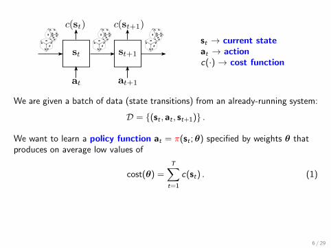
st → current stateat → actionc(·) → cost function

We are given a batch of data (state transitions) from an already-running system:

D = {(st , at , st+1)} .

We want to learn a policy function at = π(st ;θ) specified by weights θ thatproduces on average low values of

cost(θ) =T∑t=1

c(st) . (1)

Approach:

1 Learn a model for p(st+1|st , at = π(st ;θ)).

2 Minimize (1) across state trajectories (rollouts) generated by the model.

3 / 29

st → current stateat → actionc(·) → cost function

We are given a batch of data (state transitions) from an already-running system:

D = {(st , at , st+1)} .

We want to learn a policy function at = π(st ;θ) specified by weights θ thatproduces on average low values of

cost(θ) =T∑t=1

c(st) . (1)

Approach:

1 Learn a model for p(st+1|st , at = π(st ;θ)).

2 Minimize (1) across state trajectories (rollouts) generated by the model.

4 / 29

st → current stateat → actionc(·) → cost function

We are given a batch of data (state transitions) from an already-running system:

D = {(st , at , st+1)} .

We want to learn a policy function at = π(st ;θ) specified by weights θ thatproduces on average low values of

cost(θ) =T∑t=1

c(st) . (1)

Approach:

1 Learn a model for p(st+1|st , at = π(st ;θ)).

2 Minimize (1) across state trajectories (rollouts) generated by the model.

5 / 29

st → current stateat → actionc(·) → cost function

We are given a batch of data (state transitions) from an already-running system:

D = {(st , at , st+1)} .

We want to learn a policy function at = π(st ;θ) specified by weights θ thatproduces on average low values of

cost(θ) =T∑t=1

c(st) . (1)

Approach:

1 Learn a model for p(st+1|st , at = π(st ;θ)).

2 Minimize (1) across state trajectories (rollouts) generated by the model.

6 / 29

st → current stateat → actionc(·) → cost function

We are given a batch of data (state transitions) from an already-running system:

D = {(st , at , st+1)} .

We want to learn a policy function at = π(st ;θ) specified by weights θ thatproduces on average low values of

cost(θ) =T∑t=1

c(st) . (1)

Approach:

1 Learn a model for p(st+1|st , at = π(st ;θ)).

2 Minimize (1) across state trajectories (rollouts) generated by the model.

7 / 29

What model to use for the stochastic dynamics?

Classic control theory assumes the most general of dynamical systems:

st+1 = f (st , at , zt ;W) , zt → stochastic disturbance ,

where f is a deterministic function parameterized by W.

In practice most works assume additive Gaussian noise:

st+1 = f (st , at ;W) + εt , εt ∼ N (0,Γ) .

We instead keep full generality and do not remove zt :

st+1 = f (st , at , zt ;W) + εt , zt ∼ N (0, 1), εt ∼ N (0,Γ) .

8 / 29

What model to use for the stochastic dynamics?

Classic control theory assumes the most general of dynamical systems:

st+1 = f (st , at , zt ;W) , zt → stochastic disturbance ,

where f is a deterministic function parameterized by W.

In practice most works assume additive Gaussian noise:

st+1 = f (st , at ;W) + εt , εt ∼ N (0,Γ) .

We instead keep full generality and do not remove zt :

st+1 = f (st , at , zt ;W) + εt , zt ∼ N (0, 1), εt ∼ N (0,Γ) .

9 / 29

What model to use for the stochastic dynamics?

Classic control theory assumes the most general of dynamical systems:

st+1 = f (st , at , zt ;W) , zt → stochastic disturbance ,

where f is a deterministic function parameterized by W.

In practice most works assume additive Gaussian noise:

st+1 = f (st , at ;W) + εt , εt ∼ N (0,Γ) .

We instead keep full generality and do not remove zt :

st+1 = f (st , at , zt ;W) + εt , zt ∼ N (0, 1), εt ∼ N (0,Γ) .

10 / 29

Noise can have a significant effect in the optimal control. The drunken spider:

In industrial systems noise can arisefrom partial observability.

The zt are unobserved factors thataffect the dynamics in complex ways.

With no noise (alcohol), the optimal trajectory is to walk over the bridge.When noise is present, the optimal control is to walk around the lake.

Figure source H. J. Kappen, Path integrals and symmetry breaking for optimal control theory, 2008.

11 / 29

Noise can have a significant effect in the optimal control. The drunken spider:

In industrial systems noise can arisefrom partial observability.

The zt are unobserved factors thataffect the dynamics in complex ways.

With no noise (alcohol), the optimal trajectory is to walk over the bridge.When noise is present, the optimal control is to walk around the lake.

Figure source H. J. Kappen, Path integrals and symmetry breaking for optimal control theory, 2008.

12 / 29

Noise can have a significant effect in the optimal control. The drunken spider:

In industrial systems noise can arisefrom partial observability.

The zt are unobserved factors thataffect the dynamics in complex ways.

With no noise (alcohol), the optimal trajectory is to walk over the bridge.When noise is present, the optimal control is to walk around the lake.

Figure source H. J. Kappen, Path integrals and symmetry breaking for optimal control theory, 2008.

13 / 29

st+1 = f (st , at , zt ;W) + εt , zt ∼ N (0, 1), εt ∼ N (0,Γ) .

Model f using Bayesian neural network, learn posterior distribution for W and the zt .

Likelihood:

p(Y |X,Γ,W, z) =N∏

n=1

[N (yn | f (xn, zn;W),Γ) ] .

Priors:

p(W) = N (W | 0, I) , p(z) = N (z |0, I) .

Posterior:

p(W,z |Y,X,Γ) = p(Y |X,Γ,W, z)p(W)p(z)

p(Y |X,Γ) .

Predictive distribution:

p(y? | x?,Y,X,Γ) =

∫N (y? | f (x?, z?;W),Γ)N (z?|0, 1)p(W,z |Y,X,Γ) dW dz dz? .

14 / 29

st+1 = f (st , at , zt ;W) + εt , zt ∼ N (0, 1), εt ∼ N (0,Γ) .

Model f using Bayesian neural network, learn posterior distribution for W and the zt .

Likelihood:

p(Y |X,Γ,W, z) =N∏

n=1

[N (yn | f (xn, zn;W),Γ) ] .

Priors:

p(W) = N (W | 0, I) , p(z) = N (z |0, I) .

Posterior:

p(W,z |Y,X,Γ) = p(Y |X,Γ,W, z)p(W)p(z)

p(Y |X,Γ) .

Predictive distribution:

p(y? | x?,Y,X,Γ) =

∫N (y? | f (x?, z?;W),Γ)N (z?|0, 1)p(W,z |Y,X,Γ) dW dz dz? .

15 / 29

st+1 = f (st , at , zt ;W) + εt , zt ∼ N (0, 1), εt ∼ N (0,Γ) .

Model f using Bayesian neural network, learn posterior distribution for W and the zt .

Likelihood:

p(Y |X,Γ,W, z) =N∏

n=1

[N (yn | f (xn, zn;W),Γ) ] .

Priors:

p(W) = N (W | 0, I) , p(z) = N (z |0, I) .

Posterior:

p(W,z |Y,X,Γ) = p(Y |X,Γ,W, z)p(W)p(z)

p(Y |X,Γ) .

Predictive distribution:

p(y? | x?,Y,X,Γ) =

∫N (y? | f (x?, z?;W),Γ)N (z?|0, 1)p(W,z |Y,X,Γ) dW dz dz? .

16 / 29

st+1 = f (st , at , zt ;W) + εt , zt ∼ N (0, 1), εt ∼ N (0,Γ) .

Model f using Bayesian neural network, learn posterior distribution for W and the zt .

Likelihood:

p(Y |X,Γ,W, z) =N∏

n=1

[N (yn | f (xn, zn;W),Γ) ] .

Priors:

p(W) = N (W | 0, I) , p(z) = N (z |0, I) .

Posterior:

p(W,z |Y,X,Γ) = p(Y |X,Γ,W, z)p(W)p(z)

p(Y |X,Γ) .

Predictive distribution:

p(y? | x?,Y,X,Γ) =

∫N (y? | f (x?, z?;W),Γ)N (z?|0, 1)p(W,z |Y,X,Γ) dW dz dz? .

17 / 29

st+1 = f (st , at , zt ;W) + εt , zt ∼ N (0, 1), εt ∼ N (0,Γ) .

Model f using Bayesian neural network, learn posterior distribution for W and the zt .

Likelihood:

p(Y |X,Γ,W, z) =N∏

n=1

[N (yn | f (xn, zn;W),Γ) ] .

Priors:

p(W) = N (W | 0, I) , p(z) = N (z |0, I) .

Posterior:

p(W,z |Y,X,Γ) = p(Y |X,Γ,W, z)p(W)p(z)

p(Y |X,Γ) .

Predictive distribution:

p(y? | x?,Y,X,Γ) =

∫N (y? | f (x?, z?;W),Γ)N (z?|0, 1)p(W,z |Y,X,Γ) dW dz dz? .

18 / 29

st+1 = f (st , at , zt ;W) + εt , zt ∼ N (0, 1), εt ∼ N (0,Γ) .

Model f using Bayesian neural network, learn posterior distribution for W and the zt .

Likelihood:

p(Y |X,Γ,W, z) =N∏

n=1

[N (yn | f (xn, zn;W),Γ) ] .

Priors:

p(W) = N (W | 0, I) , p(z) = N (z |0, I) .

Posterior:

p(W,z |Y,X,Γ) = p(Y |X,Γ,W, z)p(W)p(z)

p(Y |X,Γ) .

Predictive distribution:

p(y? | x?,Y,X,Γ) =

∫N (y? | f (x?, z?;W),Γ)N (z?|0, 1)p(W,z |Y,X,Γ) dW dz dz? .

19 / 29

We approximate p(W,z |Y,X,Γ) with a factorized Gaussian distribution q(W, z).

The marginal means and variances of q are adjusted by minimizing α-divergences:

VariationalBayes

0.5 10

q tends to fit a mode of p q tends to fit p globally

Expectationpropagation

20 / 29

We approximate p(W,z |Y,X,Γ) with a factorized Gaussian distribution q(W, z).

The marginal means and variances of q are adjusted by minimizing α-divergences:

VariationalBayes

0.5 10

q tends to fit a mode of p q tends to fit p globally

Expectationpropagation

21 / 29

We approximate p(W,z |Y,X,Γ) with a factorized Gaussian distribution q(W, z).

The marginal means and variances of q are adjusted by minimizing α-divergences:

VariationalBayes

0.5 10

q tends to fit a mode of p q tends to fit p globally

Expectationpropagation

22 / 29

Predictions on toy problems

23 / 29

Results on wetchicken problem

24 / 29

Results on industrial benchmark

0 20 40 60 80Time

118

299

480

R(t

)

MLPsamples

sample mean

ground truth

0 20 40 60 80Time

118

299

480

R(t

)

V Bsamples

sample mean

ground truth

0 20 40 60 80Time

118

299

480

R(t

)

α = 0.5samples

sample mean

ground truth

0 20 40 60 80Time

196

514

831

R(t

)

MLPsamples

sample mean

ground truth

0 20 40 60 80Time

196

514

831

R(t

)

V Bsamples

sample mean

ground truth

0 20 40 60 80Time

196

514

831

R(t

)

α = 0.5samples

sample mean

ground truth

25 / 29

Test log-likelihood and policy performance

Average test log-likelihood:

Dataset MLP VB α=0.5 α=1.0 GPWetChicken -1.755±0.003 -1.140±0.033 -1.057±0.014 -1.070±0.011 -1.722±0.011Turbine -0.868±0.007 -0.775±0.004 -0.746±0.013 -0.774±0.015 -2.663±0.131Industrial 0.767±0.047 1.132±0.064 1.328±0.108 1.326±0.098 0.724±0.04Avg. Rank 4.3±0.12 2.6±0.16 1.3±0.15 2.1±0.18 4.7±0.12

Average policy reward:

Dataset MLP VB α=0.5 α=1.0 GPWetchicken -2.71±0.09 -2.67±0.10 -2.37±0.01 -2.42±0.01 -3.05±0.06Turbine -0.65±0.14 -0.45±0.02 -0.41±0.03 -0.55±0.08 -0.64±0.18Industrial -183.5±4.1 -180.2±0.6 -174.2±1.1 -171.1±2.1 -285.2±20.5Avg. Rank 3.6±0.3 3.1±0.2 1.5±0.2 2.3±0.3 4.5±0.3

26 / 29

Test log-likelihood and policy performance

Average test log-likelihood:

Dataset MLP VB α=0.5 α=1.0 GPWetChicken -1.755±0.003 -1.140±0.033 -1.057±0.014 -1.070±0.011 -1.722±0.011Turbine -0.868±0.007 -0.775±0.004 -0.746±0.013 -0.774±0.015 -2.663±0.131Industrial 0.767±0.047 1.132±0.064 1.328±0.108 1.326±0.098 0.724±0.04Avg. Rank 4.3±0.12 2.6±0.16 1.3±0.15 2.1±0.18 4.7±0.12

Average policy reward:

Dataset MLP VB α=0.5 α=1.0 GPWetchicken -2.71±0.09 -2.67±0.10 -2.37±0.01 -2.42±0.01 -3.05±0.06Turbine -0.65±0.14 -0.45±0.02 -0.41±0.03 -0.55±0.08 -0.64±0.18Industrial -183.5±4.1 -180.2±0.6 -174.2±1.1 -171.1±2.1 -285.2±20.5Avg. Rank 3.6±0.3 3.1±0.2 1.5±0.2 2.3±0.3 4.5±0.3

27 / 29

Conclusions

Flexible models for stochastic dynamics are important for policy learning.

In particular,

1 flexibility and scalability can be achieved by using Bayesian neuralnetworks (BNNs) with stochastic input disturbances.

2 accurate approximate Bayesian inference can be obtained by minimizingα-divergences with α = 0.5.

3 we obtain state-of-the-art policies in industrial problems by optimizingacross rollouts sampled from our BNNs.

28 / 29

Thanks!

29 / 29