Learning by Appraising:

An Emotion-based Approach to Intrinsic Reward Design ∗

Pedro Sequeira Francisco S. Melo Ana Paiva

INESC-ID / Instituto Superior Tecnico, University of Lisbon

2744-016 Porto Salvo, Portugal

Tel: +351 214 233 553

pedro.sequeira@gaips.inesc-id.pt,

{fmelo,ana.paiva}@inesc-id.pt

Abstract

In this paper, we investigate the use of emotional information in the learning process of autonomous agents.

Inspired by four dimensions that are commonly postulated by appraisal theories of emotions, we construct a

set of reward features to guide the learning process and behaviour of a reinforcement learning (RL) agent

that inhabits an environment of which it has only limited perception. Much like what occurs in biological

agents, each reward feature evaluates a particular aspect of the (history of) interaction of the agent history

with the environment, thereby in a sense replicating some aspects of appraisal processes observed in humans

and other animals. Our experiments in several foraging scenarios demonstrate that by optimising the relative

contributions of each reward feature, the resulting “emotional” RL agents perform better than standard goal-

oriented agents, particularly in consideration of their inherent perceptual limitations. Our results support

the claim that biological evolutionary adaptive mechanisms such as emotions can provide crucial clues in

creating robust, general-purpose reward mechanisms for autonomous artificial agents, thereby allowing them

to overcome some of the challenges imposed by their inherent limitations.

1 Introduction

From a computational perspective, reinforcement learning (RL) is concerned with providing efficient algorithms

that enable artificial agents to acquire new tasks through trial and error (Kaelbling et al., 1996; Sutton and Barto,

1998). Through a process of repeated interactions with its environment, an RL agent experiments with different

actions, observes their effect on the environment, and receives evaluative feedback (in the form of a numerical

reinforcement signal) about how well it is performing with respect to some unknown target task. Inspired by

∗Accepted manuscript version. The final publication, DOI 10.1177/1059712314543837, is available online athttp://adb.sagepub.com/content/early/2014/09/18/1059712314543837.

1

behaviourist psychology theories, RL algorithms are a natural choice when designing autonomous agents that

must adapt their behaviour to their environment (Sutton and Barto, 1998).

However, in deploying an RL agent, the agent designer is faced with a number of design challenges that

critically impact the performance of the agent. The first (and perhaps most fundamental) challenge is an agent-

modelling challenge: RL agents are characterised by their state in the environment, and the state should contain

all relevant information for the agent to select the best possible action. Then, at each decision step, the agent

should observe the current state, select one possible action from its repertoire, observe the impact of this action

in terms of both the resulting state and the received reinforcement signal, and adjust its action selection strategy

accordingly (Sutton and Barto, 1998). Unfortunately, it is often not possible for the agent designer to provide

the agent with the ability to observe the whole state. Considering this limitation, the designer may decide to

either consider a more complex model that explicitly accommodates for the perceptual limitations of the agent

(Kaelbling et al., 1998) or to ignore these limitations and treat whatever information is available as the agents

complete state (Jaakkola et al., 1995).

A second challenge that the designer faces is a task-modelling challenge: given the adopted representation

for the (state of the) agent, the designer must design the reinforcement signal that enables the agent to learn

the intended task as efficiently as possible. The design of reward functions is a difficult endeavour and has been

the topic of intense research in the RL literature, which has lead to interesting results regarding both inverse

reinforcement learning (Ng and Russell, 2000; Ramachandran and Amir, 2007) and reward shaping (Ng et al.,

1999; Wiewiora, 2003).

Recent research regarding the origin of rewards in nature (Singh et al., 2009) and intrinsically motivated

reinforcement learning (IMRL, Singh et al., 2010) has led to the formulation of the optimal reward problem (ORP)

to address the task-modelling challenge discussed above. Roughly speaking, the ORP involves the discovery of a

reward function from a set of possible rewards, which should induce the best “lifelong behaviour” possible for the

agent in a set of environments of interest, as measured in terms of a target task.

Interestingly, results have indicated that by selecting the reward that best “solves” the ORP, it is often the

case that both the agent- and task-modelling challenges can be successfully addressed (Sorg et al., 2010b). In

particular, it is often possible to select a reward that not only enables the agent to learn the desired task in an

efficient manner but also, as part of that process, mitigates the impact of the agent’s inherent limitations on

its ability to successfully perform the task. Intuitively, the reward is used to provide the agent with implicit

information about (parts of) the state that the agent would be unable to perceive otherwise. The ORP thus

provides an appealing framework within which the RL agent designer can reason about rewards while alleviating

part of the modelling burden associated with selecting good state representations.

However, the ORP raises a new design challenge: that of designing a rich set of possible rewards for the task

at hand from which to select such an informative reward. Such an endeavour often involves significant domain

knowledge, and several possibilities have been considered in the literature, which require varying levels of manual

adjustments (Bratman et al., 2012; Niekum et al., 2010; Singh et al., 2010; Sorg et al., 2010a).

2

In this paper, we investigate the nature of the rewards to be considered in addressing the ORP. In particular,

we want to construct a set of possible rewards that is general enough to alleviate the need for excessive adjustments

across domains and also informative enough to provide useful information for each specific domain. We address the

ORP within the framework of intrinsically motivated RL (IMRL), in which the process of reward optimisation is

interpreted as a computational counterpart to the evolutionary process that crafted reinforcement mechanisms in

animals (Singh et al., 2010). Drawing inspiration from natural systems, we consider intrinsic reward mechanisms

inspired by appraisal theories of emotions.

In a previous paper (Sequeira et al., 2011a), we performed a preliminary study of the impact of emotion-based

rewards on intrinsically motivated agents. In this paper, we focus on the design of a general-purpose reward

mechanism and its impact on alleviating the demand for having to design specific rewards for different domains.

The main technical contribution is the integration of a mechanism within IMRL that provides a reward built from

a set of four domain-independent emotion-based features, namely, novelty, valence, goal relevance and control, each

of which are inspired by a dimension of appraisal of the emotional significance of events and are commonly found

in the psychology literature (Ellsworth and Scherer, 2003; Lazarus, 2001; Leventhal and Scherer, 1987; Roseman

and Smith, 2001; Scherer, 2001). We perform such a mapping regardless of its validity in terms of appraisal

theories, but we redesigned many of the previously proposed features to focus on emotions as a plausible source of

such general-purpose and domain-independent intrinsic reward and discuss possible alternatives for each feature.

We illustrate the usefulness of the proposed reward design by comparing the performance of our “emotion-

driven” RL agents with that of standard, goal-driven RL agents in several experiments that feature foraging

scenarios. In addition, we extend our previous work by investigating the impact of maladaptive behaviours on

the agent’s performance and the emergence of “universal” agents that behave well, on average, in all scenarios.

2 Related Work

Early artificial intelligence (AI) research was mostly focused on the reproduction of human reasoning processes,

e.g., by building systems that could prove theorems (Newell and Simon, 1956), solve algebra word problems

(Bobrow, 1964) or understand English sentences (Winograd, 1971). Pioneering AI researchers also emphasised

the role of emotional processes as an attention-focusing, task-prioritising mechanism that is crucial to any system

that is to be regarded as intelligent (Minsky, 1986; Simon, 1967). Developments in neurophysiology brought

prominence to the role of emotions in cognition (Damasio, 1994) and prompted in the AI community to develop

computational models of emotions, which are usually based on appraisal theories of emotions (Marsella et al.,

2010). Many works in the area of affective computing (AC) address the impact of emotional processes on decision-

making to create more engaging interactive artificial agents (Picard, 2000).

Within the area of AC, several works combine learning and emotional mechanisms in a complementary manner

to create artificial agents that exhibit richer behaviour. For example, the FLAME model uses RL to build

emotion-object associations and predict the user’s actions (El-Nasr et al., 2000). Another example is the work

3

of Armony et al. (1997), in which connectionist learning is used to emulate effects that are commonly associated

with fear conditioning. The artificial creatures of Canamero (1997) also use “low-level” emotional signals that

drive behaviour selection. Jacobs et al. (2014) derive emotions of “joy”, “distress”, “hope” and “fear” from signals

generated by the RL algorithm and demonstrate that the results of agent-based simulations are able to replicate

psychological and behavioural dynamics of emotion.

Another line of work, which is more closely related to our own, uses emotions to actually influence decision-

making within RL. Gadanho (2003) propose a bottom-up approach to emotion elicitation. Their system uses

artificial neural networks to determine a dominant emotional state. A measure of wellbeing (or valence) is

calculated for each state by computing the relative change in the value of a set of homeostatic variables (energy,

welfare and activity) and also accounting for predictions associated with that state. RL is used to learn state-

behaviour associations, and the rewards are provided by the intensity and valence of the current dominant emotion.

Salichs and Malfaz (2006) propose a set of basic emotions to control the behaviour of an RL agent. In their

model, the reward depends on variations of the agent’s wellbeing. Their behaviour-selection mechanism uses

a predefined level of “dare” that determines a preference for conservative (high-valued) actions over bad (low-

valued) actions due to “fear”. Marinier et al. (2009) propose an intrinsic reward signal based on the appraisal of

conduciveness that determines the sign of the reward value, whereas the intensity of the agent’s current feeling

determines the magnitude of the signal. An experiment conducted in a grid-world scenario demonstrated that

intermediate, emotion-based rewards lead to learning the task faster. Broekens et al. (2007) propose associating

positive affective states with exploitation and negative states with exploration. They demonstrated that this

model provides adaptive benefits for RL agents in specific scenarios.1 The affective state and reward depend on

the relation between the short and long-term running averages of past reinforcement signals. Following this work,

Hogewoning et al. (2007) use a chi-square statistical test to compute the significance of the differences between

these two averages to influence action selection.

The work that is most similar to our proposed approach is that of Ahn and Picard (2006). In that work, the

authors consider the use of extrinsic and intrinsic rewards both to improve the learning performance of the agent

and to influence decision-making. The extrinsic reward relates to external goals, and the paper proposes a model

for an affective anticipatory reward that is based on valence and arousal levels.

Much like in the work of Ahn and Picard (2006), our approach complements the (extrinsic) reward signal

provided by the environment with an intrinsic reward signal that is constructed from a set of features based

on major dimensions of emotional appraisal. In a sense, these features provide, at each time-step, a dynamical

representation of the “emotional state” of the agent. This aspect is in contrast with most surveyed works, which

rely either on a predefined set of discrete emotions or scalar evaluations of the emotional state of the agent.2

Additionally, unlike Ahn and Picard (2006), we do not treat the external and internal rewards differently.

1Interestingly, such results contrast with common RL approaches, such as UCB (Auer et al., 2002), E3 (Kearns and Singh, 2002),and R-MAX (Brafman, 2003), that rely on the principle of “optimism in the face of uncertainty”.

2We note that, in this paper, we are not concerned with labelling the emotional state of the agent as “happy”, “sad” or “angry”.However, one can envisage a labelling mechanism that partitions the agent’s “emotional space” into regions, with each correspondingto a specific emotional label.

4

Instead, they are harmoniously combined to yield a single reward signal that guides the agent’s behaviour. The

trade-off between such external and internal rewards is “fit” for the class of environments that the agent expects

to encounter. A related optimisation can be found in biological agents, which process emotional states differently

depending on their survival needs (Frijda and Mesquita, 1998; Roseman and Smith, 2001; Smith and Kirby, 2009).

Moreover, we do not rely on predefined associations between emotional states and actions. Instead, the agent

learns from the (combined) intrinsic rewards an action selection rule that optimises the balanced benefit that

arises from the environment and the agent’s internal state.

We also refer to our work in (Sequeira et al., 2014), which complements this paper. In that work, we test the

emergence of emotion-related rewards by using evolutionary computation mechanisms. In other words, in this

paper, we depart from the emotional appraisal literature to manually design reward features that have evaluative

characteristics that are similar to those ascribed by some appraisal dimensions, whereas in (Sequeira et al., 2014),

we use genetic programming to determine a set of domain-independent reward features and then analyse the

dynamical and structural properties of those features in consideration of appraisal theories.

3 Background

This section describes the decision-theoretic framework within which we introduce our contributions. We discuss

the models used throughout the paper to describe our agents and present the basic nomenclature and notation.

3.1 (Partially Observable) Markov Decision Problems

In its most general form, the sequential decision problem faced by RL agents can be modelled as a partially

observable Markov decision problem (POMDP) (Kaelbling et al., 1998), which is denoted as a tuple M =

(S,A,Z,P,O, r, γ). At each discrete time-step t = 0, 1, 2, 3, . . ., the environment is described by some state,

which is represented as a random variable (r.v.) St that takes values from a finite set of possible states, S. The

agent makes an observation, which is denoted as a r.v. Zt that takes values from a set of possible observations,

Z, that depends on the state St but that is often insufficient for the agent to unambiguously infer St. The

agent then performs some action (which is denoted as a r.v. At ∈ A), and the environment transitions to state

St+1. This transition is governed by the probabilities P [St+1 = s′ | St = s,At = a] = P(s′ | s, a). The agent then

receives a numerical reward, r(St, At), that represents the desirability of executing action At in state St (in terms

of the target task) and makes a new observation Zt+1, after which the process repeats. The observations Zt of

the agent are governed by the probabilities P [Zt+1 = z | St+1 = s,At = a] = O(z | s, a). Traditional approaches

to RL mainly focus on scenarios in which the observations Zt allow the agent to unambiguously determine the

underlying state St. Such scenarios are said to have full observability, and the POMDP parameters Z and O can

be safely ignored. The resulting model, which is represented as a tuple M = (S,A,P, r, γ), is simply referred to

as a Markov decision problem (MDP).

5

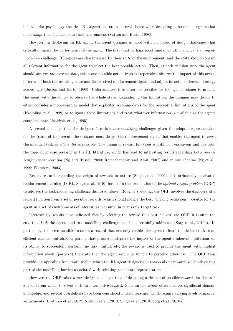
In the traditional view of RL, the reward r(s, a)3 “evaluates” the agent’s behaviour with respect to the task

it must (learn to) perform, thereby acting as a critic that resides in the (external) environment, as depicted in

Fig. 1(a) (Singh et al., 2010). The goal of the agent is to select its actions to gather as much reward as possible

during its lifetime, where the reward is discounted by some factor (Kaelbling et al., 1996; Sutton and Barto, 1998).

In an MDP, a policy is a decision-rule π : S → A that determines the action to be executed in each state

s ∈ S. We can associate with each MDP policy π a value function, V π : S → R, that determines, for each initial

state s ∈ S, the value that the agent expects to receive by choosing its actions according to π. The value function

is

V π(s) = Eπ

[∑t

γtr(St, At) | S0 = s

], (1)

where γ is a positive discount value such that γ < 1. An optimal policy is defined as any policy π∗ such that

V π∗(s) ≥ V π(s) for any state s ∈ S and policy π. The existence of one such policy can be guaranteed under mild

assumptions regarding the MDP (Puterman, 1994). We can also associate with π∗ a function Q∗ : S × A → R

that verifies the recursive relation

Q∗(s, a) = r(s, a) + γ∑s′∈S

P(s′ | s, a) maxa′∈A

Q∗(s′, a′). (2)

Q∗ determines how good (in the long-run) each action is in each possible state faced by the agent, given that the

latter performs optimally afterwards, and can be computed by iterating over (2) using a dynamic programming

approach that is known as value iteration. Computation of Q∗ using value iteration requires knowledge of the

MDP parameters, namely, r and P. Reinforcement learning typically addresses situations in which one or both

of these parameters are unknown. In those situations, the agent must learn the optimal policy by relying on data

collected from the environment, either online (Watkins, 1989) or offline (Ernst et al., 2005).

In this paper, we consider RL agents that follow the prioritised sweeping algorithm (Moore and Atkeson,

1993), which is an online RL algorithm that uses the data collected from the environment to construct estimates

P and r of the parameters of the MDP. Such estimates are then used to perform, at each time-step, multiple value

iteration updates using a well-defined update schedule (which is implemented using a priority queue).

3.2 Intrinsically Motivated RL and the ORP

The RL paradigm described in Section 3.1 departs from a (PO)MDP model by describing a sequential problem

faced by a decision-maker in a dynamic and uncertain world in which the task is implicitly encoded in the reward

r. The performance of the agent depends on the ability of r to convey information about the task to be learned,

and several works in the literature have addressed the problem of reward design. One approach relies on the idea

of shaping (Mataric, 1994; Ng et al., 1999; Randløv and Alstrøm, 1998): given a reward r that encodes some

target task, shaping consists of applying some transformation to r, thereby yielding a second reward, r′, that

encodes the same task but is more informative for a learning agent. A second and more recent approach is to first

3When there is no danger of confusion, we abusively refer to a reward function r simply as a reward.

6

Environment

Agent

RL

Sensors

State Action

Perceptions

Critic

Rewards

(a) Traditional RL framework

Environment

Agent

RL

Sensors

State

Rewardsignals

Action

Perceptions

Int. env.

Critic

r

(b) IMRL framework

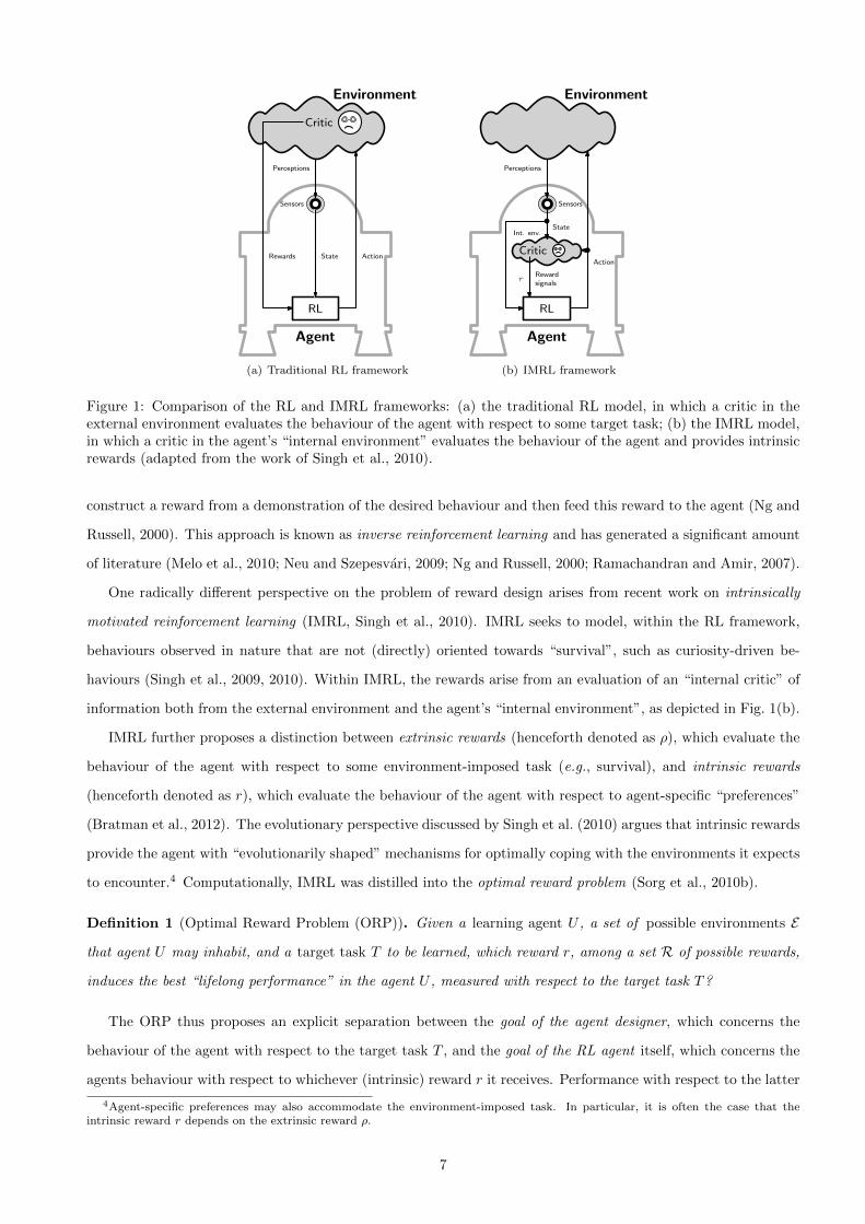
Figure 1: Comparison of the RL and IMRL frameworks: (a) the traditional RL model, in which a critic in theexternal environment evaluates the behaviour of the agent with respect to some target task; (b) the IMRL model,in which a critic in the agent’s “internal environment” evaluates the behaviour of the agent and provides intrinsicrewards (adapted from the work of Singh et al., 2010).

construct a reward from a demonstration of the desired behaviour and then feed this reward to the agent (Ng and

Russell, 2000). This approach is known as inverse reinforcement learning and has generated a significant amount

of literature (Melo et al., 2010; Neu and Szepesvari, 2009; Ng and Russell, 2000; Ramachandran and Amir, 2007).

One radically different perspective on the problem of reward design arises from recent work on intrinsically

motivated reinforcement learning (IMRL, Singh et al., 2010). IMRL seeks to model, within the RL framework,

behaviours observed in nature that are not (directly) oriented towards “survival”, such as curiosity-driven be-

haviours (Singh et al., 2009, 2010). Within IMRL, the rewards arise from an evaluation of an “internal critic” of

information both from the external environment and the agent’s “internal environment”, as depicted in Fig. 1(b).

IMRL further proposes a distinction between extrinsic rewards (henceforth denoted as ρ), which evaluate the

behaviour of the agent with respect to some environment-imposed task (e.g., survival), and intrinsic rewards

(henceforth denoted as r), which evaluate the behaviour of the agent with respect to agent-specific “preferences”

(Bratman et al., 2012). The evolutionary perspective discussed by Singh et al. (2010) argues that intrinsic rewards

provide the agent with “evolutionarily shaped” mechanisms for optimally coping with the environments it expects

to encounter.4 Computationally, IMRL was distilled into the optimal reward problem (Sorg et al., 2010b).

Definition 1 (Optimal Reward Problem (ORP)). Given a learning agent U , a set of possible environments E

that agent U may inhabit, and a target task T to be learned, which reward r, among a set R of possible rewards,

induces the best “lifelong performance” in the agent U , measured with respect to the target task T?

The ORP thus proposes an explicit separation between the goal of the agent designer, which concerns the

behaviour of the agent with respect to the target task T , and the goal of the RL agent itself, which concerns the

agents behaviour with respect to whichever (intrinsic) reward r it receives. Performance with respect to the latter

4Agent-specific preferences may also accommodate the environment-imposed task. In particular, it is often the case that theintrinsic reward r depends on the extrinsic reward ρ.

7

goal, as is standard in RL, is usually measured in terms of the total discounted (intrinsic) reward accumulated

over time. As for the former goal, we start by observing that the behaviour of the agent is defined by (i) the

POMDP used to model the environment with which the agent interacts and (ii) the decision algorithm used by

the agent. Together, they specify the set of possible interactions that the agent can experience.

Formally, let H denote the set of all possible finite histories that the agent can experience throughout its

lifetime. In particular, we consider an element h ∈ H as a sequence h1:t = {z1, a1, ρ1, z2, . . . , at−1, ρt−1, zt}, where

zτ , aτ and ρτ denote, respectively, the observation at time-step τ , the action selected at time-step τ , and the

extrinsic reward at time-step τ . Referring back to Fig. 1(b), the internal critic is responsible for processing the

agent’s perceptions into a history h that contains information about the environment (in the form of a sequence

{z1, . . . , zt}) and information about the extrinsic reward (in the form of a sequence {ρ1, . . . , ρt−1}).

Additionally, let r denote the intrinsic reward that drives the behaviour of the agent (which is modelled as a

POMDPM = (S,A,Z,P,O, r, γ)). We refer to the remaining parameters of the POMDP as the environment of

interest, e, and write P [h | r, e] to denote the probability of observing history h ∈ H given r and e.

We define the fitness function, f : H → R, that maps each history h ∈ H into a numerical value that evaluates

the performance of the agent with respect to the target task T . Given a space of possible rewards, R, and a

distribution penv over the set of environments, E , the ORP can thus be formulated as the problem of determining

the optimal reward r∗ ∈ R such that

r∗ = argmaxr∈R

F(r) , Ee∼penv [f(h) | r, e] , (3)

where F(r) is the expected fitness associated with reward r. In this paper, we consider the fitness of an agent U

throughout a particular history as the total extrinsic reward accumulated therein, i.e.,

f(h1:t) =

t∑τ=1

ρτ . (4)

This particular choice of fitness function implicitly indicates that ρ directly measures the fitness of the agent and,

therefore, we interchangeably refer to ρ as the extrinsic reward and the fitness-based reward.

4 Designing Emotion-based Rewards

This section introduces our main technical contribution, which consists of a set of reward features that are inspired

by four common dimensions of emotional appraisal within the IMRL framework.

4.1 Appraisal Theories of Emotions

Given the potential advantages of emotional processing mechanisms in artificial agents (Picard, 2000), we now

investigate how to port such mechanisms to the IMRL framework by considering well-established appraisal theories

of emotion (ATEs) (Arnold, 1960; Ellsworth and Scherer, 2003; Roseman and Smith, 2001).

8

Environment

Individual

Stimuli

Physiologicalreactions

Action tendencies

Emotional Response

Goals, beliefsintentions

Appraisal

Appraisaloutcome

Bodilyexpressions

Belief/desire revision

Emotion-relatedbehaviors

Person-env.relation

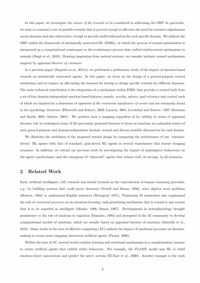
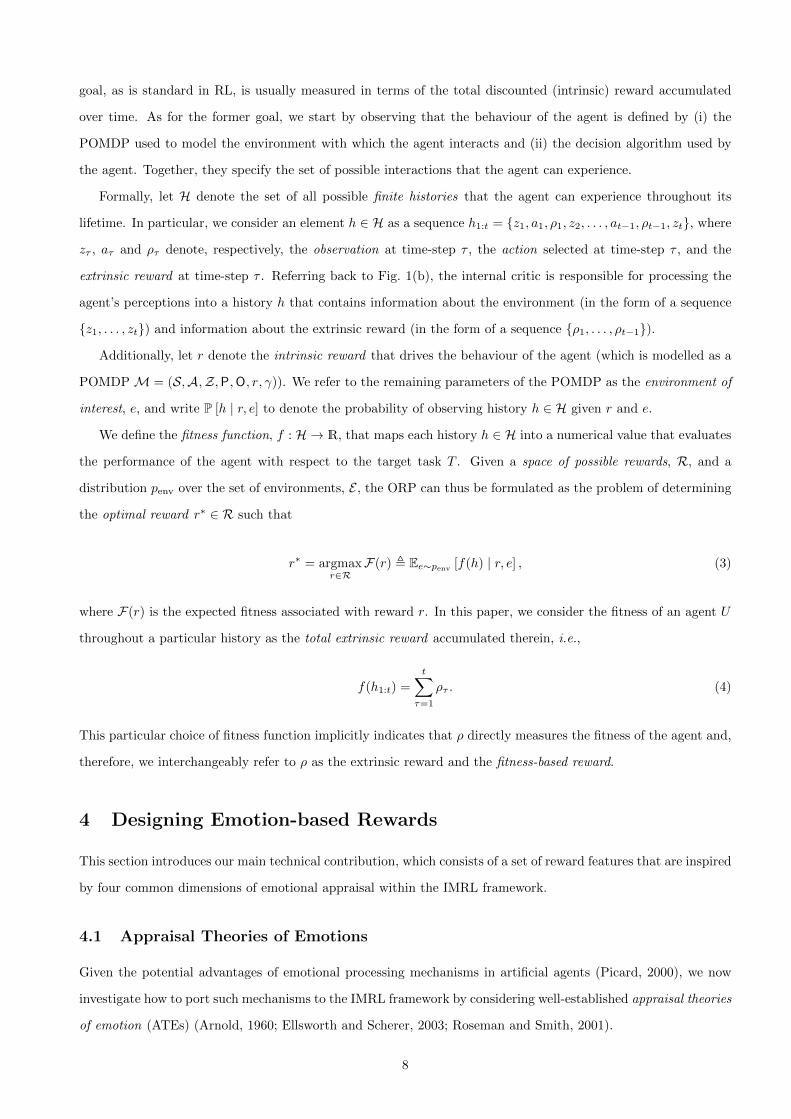
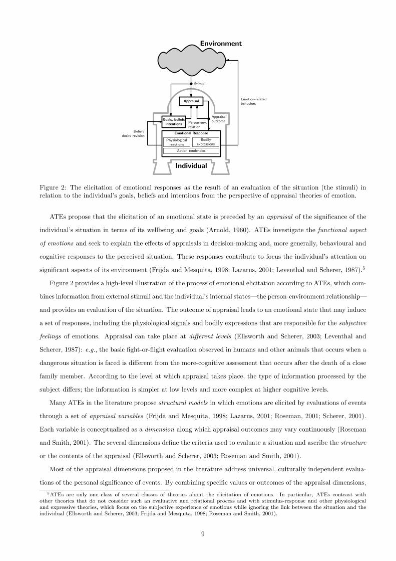
Figure 2: The elicitation of emotional responses as the result of an evaluation of the situation (the stimuli) inrelation to the individual’s goals, beliefs and intentions from the perspective of appraisal theories of emotion.

ATEs propose that the elicitation of an emotional state is preceded by an appraisal of the significance of the

individual’s situation in terms of its wellbeing and goals (Arnold, 1960). ATEs investigate the functional aspect

of emotions and seek to explain the effects of appraisals in decision-making and, more generally, behavioural and

cognitive responses to the perceived situation. These responses contribute to focus the individual’s attention on

significant aspects of its environment (Frijda and Mesquita, 1998; Lazarus, 2001; Leventhal and Scherer, 1987).5

Figure 2 provides a high-level illustration of the process of emotional elicitation according to ATEs, which com-

bines information from external stimuli and the individual’s internal states—the person-environment relationship—

and provides an evaluation of the situation. The outcome of appraisal leads to an emotional state that may induce

a set of responses, including the physiological signals and bodily expressions that are responsible for the subjective

feelings of emotions. Appraisal can take place at different levels (Ellsworth and Scherer, 2003; Leventhal and

Scherer, 1987): e.g., the basic fight-or-flight evaluation observed in humans and other animals that occurs when a

dangerous situation is faced is different from the more-cognitive assessment that occurs after the death of a close

family member. According to the level at which appraisal takes place, the type of information processed by the

subject differs; the information is simpler at low levels and more complex at higher cognitive levels.

Many ATEs in the literature propose structural models in which emotions are elicited by evaluations of events

through a set of appraisal variables (Frijda and Mesquita, 1998; Lazarus, 2001; Roseman, 2001; Scherer, 2001).

Each variable is conceptualised as a dimension along which appraisal outcomes may vary continuously (Roseman

and Smith, 2001). The several dimensions define the criteria used to evaluate a situation and ascribe the structure

or the contents of the appraisal (Ellsworth and Scherer, 2003; Roseman and Smith, 2001).

Most of the appraisal dimensions proposed in the literature address universal, culturally independent evalua-

tions of the personal significance of events. By combining specific values or outcomes of the appraisal dimensions,

5ATEs are only one class of several classes of theories about the elicitation of emotions. In particular, ATEs contrast withother theories that do not consider such an evaluative and relational process and with stimulus-response and other physiologicaland expressive theories, which focus on the subjective experience of emotions while ignoring the link between the situation and theindividual (Ellsworth and Scherer, 2003; Frijda and Mesquita, 1998; Roseman and Smith, 2001).

9

these theories can model discrete emotions (such as joy, sadness, and fear) and predict the particular physiological

responses and action tendencies that are associated with each of them (Ellsworth and Scherer, 2003; Frijda and

Mesquita, 1998; Roseman and Smith, 2001). Therefore, most ATEs largely agree regarding which dimensions

are necessary to evaluate a given situation. Ellsworth and Scherer (2003) compared the most common ATEs

and identified the following set of five major dimensions of appraisal, for which there is broad consensus in the

community and on which our approach is based: novelty, pleasantness/valence, goal relevance, power/coping

potential and normative/social significance.

4.2 Learning and Partial Observability

The presentation in Section 3 focused mostly on the benign situation in which the agent, at each time-step, is

able to completely observe the state St of the environment. However, in real-world scenarios, this is seldom the

case. For example, a robot’s perception about the state of the world is limited to the accuracy and resolution of

its sensors. The POMDP model briefly discussed above enables the agent to reason about information that its

observations yield about the actual state of the environment. Unfortunately, POMDP models are significantly

more elaborate than MDPs, both conceptually and algorithmically. In fact, while MDPs are efficiently solvable,

i.e., an optimal policy for an MDP can be computed rather efficiently (Puterman, 1994), their partially observable

counterparts were proven to be undecidable in the worst case (Madani et al., 1999).

Given the difficulty inherent in reasoning about partial observability, one possible approach is to ignore partial

observability altogether and reason about the observations of the agent as if they were actual states (Jaakkola

et al., 1995). Another approach is to rely on the agent observations to track the most likely state of the environment

and select the actions accordingly (Littman et al., 1995). In highly structured problems (e.g., robotic navigation),

this simple approach can actually yield good results (Cassandra, 1998). However, in general, such simplified

solutions are bound to lead to poor performance, as demonstrated by the work of Singh et al. (1994). Moreover,

computing the best such solution is typically a difficult problem (Littman, 1994). Other approaches to address

partial observability in RL settings that build into the agent prior knowledge that can somehow alleviate its

perceptual limitations have been proposed (Aberdeen, 2003). Examples include approaches that are based on

some form of memory (McCallum, 1995). However, such approaches typically require very specific algorithms

that are tailored to leverage information from particular aspects of the agents history (Aberdeen, 2003).

The IMRL framework discussed in Section 3.2 provides an elegant framework within which it is possible to

implicitly “supply” prior knowledge to the learning agent. In fact, by properly tuning the reward, it is possible

to induce in the agent behaviours that may not be directly related to the target task but which, in time, can

mitigate the impact of the agent’s limitations on its performance (Sorg et al., 2010b). However, as discussed in

Section 3.2, an adequately informative reward is critically dependent on the considered set of rewards, R, which

yields a new design challenge—that of designing the set R of possible rewards for a desired task. As discussed

above, this challenge often requires significant domain knowledge, and several possibilities have been considered

in the literature (Bratman et al., 2012; Niekum et al., 2010; Sorg et al., 2010a).

10

Below, we propose a set of domain-independent reward features that are inspired by appraisal theories of

emotions and can be used as building blocks to construct richer sets of reward functions.

4.3 Emotion-based Reward Design

We are now in position to introduce our main technical contribution. We depart from the discussion of ATEs in

Section 4.1 and propose a set of reward features that are inspired by each of the major dimensions of appraisal.

Going back to the IMRL agent architecture in Fig. 1(b), we recall that the internal critic provides the RL

decision-making component with reward information. This reward is, in turn, constructed using information

both from the external environment (the sensations, including the extrinsic reward) and the agent’s internal

environment. Drawing a parallel with the process of appraisal depicted in Fig. 2, we can approximately identify

the internal critic in our IMRL agent as the module in which appraisal occurs. The reward r used for learning

and decision-making approximately corresponds to the outcome of such a process.

We treat the agent’s perceptions as state, which is a common simplifying approach that was already dis-

cussed in Section 4.2. This approach is equivalent to considering, in the POMDP model, that S = Z and

P [St = s | Zt = s] = P [Zt = s | St = s] = 1. Therefore, we henceforth omit any explicit references to observations,

with the understanding that “states”, as perceived by the agent, actually correspond to POMDP observations.

In practice, as discussed above, it is seldom the case that S = Z, and our assumption will provide an opportunity

to assess the ability of our approach to overcome the impact of disregarding partial observability issues.

We consider a set of possible rewards R in which each reward r is a linear combination of some pre-defined

reward features, {φi, i = 1, . . . , N}. Each feature φi maps perception-action-history triplets (which are abusively

denoted as (s, a, h), given our treatment of perceptions as state) to a scalar value φi(s, a, h) ∈ R. For every r ∈ R,

r(s, a, h) =

N∑i=1

φi(s, a, h)θi = φ>(s, a, h)θ,

where θi is the linear coefficient that is associated with feature φi in r.

We propose that each appraisal dimension maps to a corresponding reward feature φi, i = 1, . . . , N . Much

like appraisal dimensions in biological agents, our reward features evaluate the significance of the agent’s current

situation for its “wellbeing” according to specific criteria (Singh et al., 2009, 2010). Our approach thus follows

the perspective that appraisal corresponds to a multi-dimensional, continuous-valued evaluation (Ellsworth and

Scherer, 2003; Scherer, 2001). Given the simplicity of the RL agent model considered here, our emotion-based

reward features rely on low-level statistical “summaries” of the agent’s history of interaction with the environment.

Because we are focusing on single-agent scenarios, we adopt only four of the aforementioned major dimensions

of appraisal, namely, novelty, valence, goal relevance and control (Ellsworth and Scherer, 2003).6 Our features

are constructed from information that is usually available to RL agents and are therefore general and domain-

independent. The value of each reward feature φi(s, a, h) somehow indicates the degree of activation/significance

6We refer to the work of Sequeira et al. (2011b) for a treatment of the multiagent case.

11

of dimension i associated with the execution of action a after perceiving s and given a history of interaction h.

Formally, our set of rewards, R, is the linear span of the set {φn, φr, φc, φv, φρ}, where

• φn(s, a, h) denotes the novelty associated with performing action a after observing s, given the history h;

• φr(s, a, h) denotes the goal relevance of performing action a after observing s, given h;

• φc(s, a, h) denotes the degree of control over the outcome of executing action a after observing s, given h;

• φv(s, a, h) denotes the expected valence of executing a after observing s, given history h;

• Finally, φρ(s, a, h) = ρ(s, a) is not an emotion-based feature. Rather, it corresponds to the estimated

fitness-based reward for executing a after observing s,7 ρ(s, a) = E [ρt | St = s,At = a].

Below, we describe each of the aforementioned features in detail.

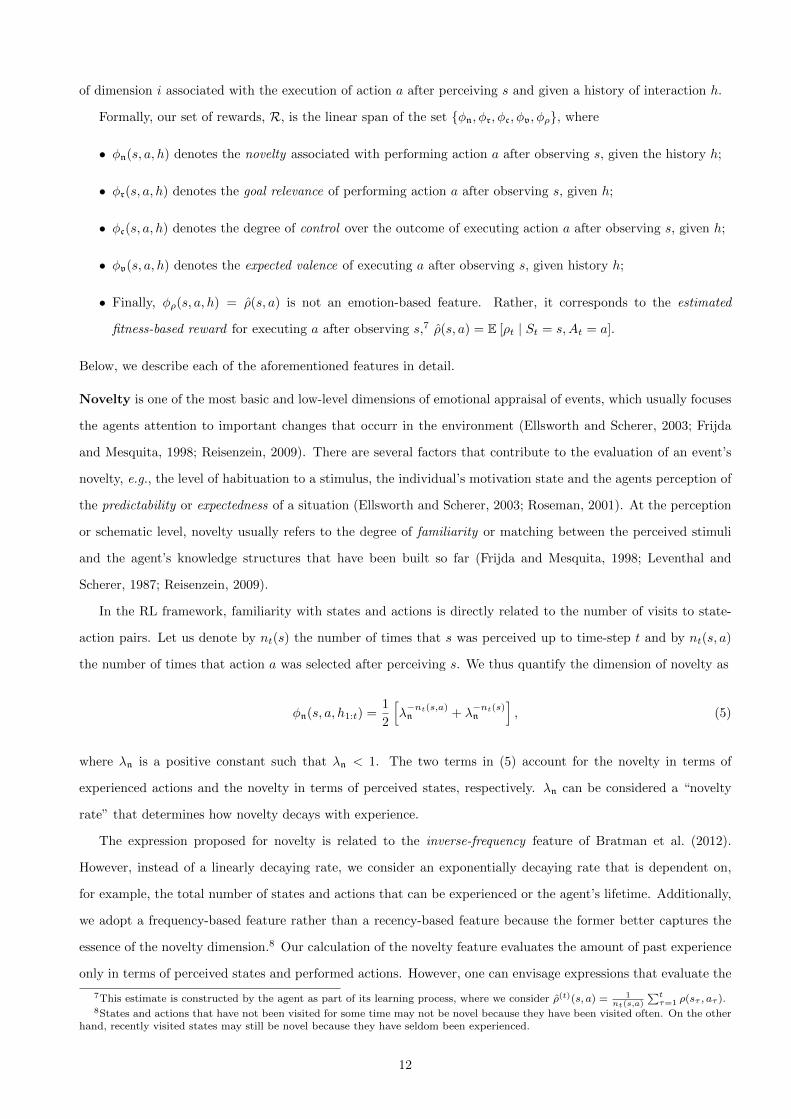
Novelty is one of the most basic and low-level dimensions of emotional appraisal of events, which usually focuses

the agents attention to important changes that occurr in the environment (Ellsworth and Scherer, 2003; Frijda

and Mesquita, 1998; Reisenzein, 2009). There are several factors that contribute to the evaluation of an event’s

novelty, e.g., the level of habituation to a stimulus, the individual’s motivation state and the agents perception of

the predictability or expectedness of a situation (Ellsworth and Scherer, 2003; Roseman, 2001). At the perception

or schematic level, novelty usually refers to the degree of familiarity or matching between the perceived stimuli

and the agent’s knowledge structures that have been built so far (Frijda and Mesquita, 1998; Leventhal and

Scherer, 1987; Reisenzein, 2009).

In the RL framework, familiarity with states and actions is directly related to the number of visits to state-

action pairs. Let us denote by nt(s) the number of times that s was perceived up to time-step t and by nt(s, a)

the number of times that action a was selected after perceiving s. We thus quantify the dimension of novelty as

φn(s, a, h1:t) =1

2

[λ−nt(s,a)n + λ

−nt(s)n

], (5)

where λn is a positive constant such that λn < 1. The two terms in (5) account for the novelty in terms of

experienced actions and the novelty in terms of perceived states, respectively. λn can be considered a “novelty

rate” that determines how novelty decays with experience.

The expression proposed for novelty is related to the inverse-frequency feature of Bratman et al. (2012).

However, instead of a linearly decaying rate, we consider an exponentially decaying rate that is dependent on,

for example, the total number of states and actions that can be experienced or the agent’s lifetime. Additionally,

we adopt a frequency-based feature rather than a recency-based feature because the former better captures the

essence of the novelty dimension.8 Our calculation of the novelty feature evaluates the amount of past experience

only in terms of perceived states and performed actions. However, one can envisage expressions that evaluate the

7This estimate is constructed by the agent as part of its learning process, where we consider ρ(t)(s, a) = 1nt(s,a)

∑tτ=1 ρ(sτ , aτ ).

8States and actions that have not been visited for some time may not be novel because they have been visited often. On the otherhand, recently visited states may still be novel because they have seldom been experienced.

12

predictability of stimuli or the probability of actions outcomes that are consistent with the corresponding novelty

dimension in biological agents (Ellsworth and Scherer, 2003; Leventhal and Scherer, 1987).

Goal Relevance assesses the relevance of a perceived event in terms of the attainment of the agent’s long-term

goals or the satisfaction of its needs (Ellsworth and Scherer, 2003; Lazarus, 2001; Leventhal and Scherer, 1987).

Also related to the notions of desire-congruence (Reisenzein, 2009) and motive-consistence (Roseman, 2001), goal

relevance is essential for the survival and adaptation of an individual to its environment (Ellsworth and Scherer,

2003; Reisenzein, 2009). Therefore, goal relevance has a motivational basis and is influenced by the importance

of the event and the consistency of its outcomes in relation to the goals or needs under consideration (Roseman,

2001). Broadly speaking, the goal relevance of an event increases if such event is consistent with or conductive

to the achievement of the individual’s goals and decreases when the consequences of the event are obstructive to

reaching those goals (Ellsworth and Scherer, 2003; Reisenzein, 2009).

At a very low level, the goal of an individual is to attain maximum fitness throughout its lifetime. Let V(t)ρ

denote the estimate, at time-step t, of the value function associated with only the fitness-based reward, φρ, which

satisfies the fixed-point relation V(t)ρ (s) = maxa∈AQ

(t)ρ (s, a), where Q

(t)ρ denotes the estimate of the action-value

function associated with only the fitness-based reward. States for which V(t)ρ is high should then be preferable over

those with a low value of V(t)ρ . We define the estimated goal state at time-step t, s

(t)ρ , as s

(t)ρ = argmaxs∈S V

(t)ρ (s)

and let dt(s) denote the estimate, at time-step t, of the number of steps needed to reach s(t)ρ from s, given the

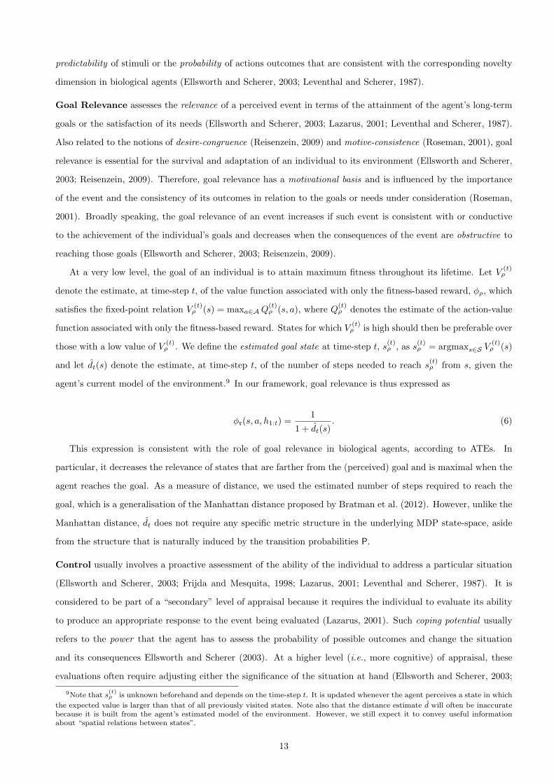
agent’s current model of the environment.9 In our framework, goal relevance is thus expressed as

φr(s, a, h1:t) =1

1 + dt(s). (6)

This expression is consistent with the role of goal relevance in biological agents, according to ATEs. In

particular, it decreases the relevance of states that are farther from the (perceived) goal and is maximal when the

agent reaches the goal. As a measure of distance, we used the estimated number of steps required to reach the

goal, which is a generalisation of the Manhattan distance proposed by Bratman et al. (2012). However, unlike the

Manhattan distance, dt does not require any specific metric structure in the underlying MDP state-space, aside

from the structure that is naturally induced by the transition probabilities P.

Control usually involves a proactive assessment of the ability of the individual to address a particular situation

(Ellsworth and Scherer, 2003; Frijda and Mesquita, 1998; Lazarus, 2001; Leventhal and Scherer, 1987). It is

considered to be part of a “secondary” level of appraisal because it requires the individual to evaluate its ability

to produce an appropriate response to the event being evaluated (Lazarus, 2001). Such coping potential usually

refers to the power that the agent has to assess the probability of possible outcomes and change the situation

and its consequences Ellsworth and Scherer (2003). At a higher level (i.e., more cognitive) of appraisal, these

evaluations often require adjusting either the significance of the situation at hand (Ellsworth and Scherer, 2003;

9Note that s(t)ρ is unknown beforehand and depends on the time-step t. It is updated whenever the agent perceives a state in which

the expected value is larger than that of all previously visited states. Note also that the distance estimate d will often be inaccuratebecause it is built from the agent’s estimated model of the environment. However, we still expect it to convey useful informationabout “spatial relations between states”.

13

Roseman, 2001) or the individual’s goals to cope with the possible outcomes of the event (Lazarus, 2001; Smith

and Kirby, 2009). At a lower level of processing, these evaluations simply assess the extent to which an event

or its outcomes are controllable and whether the individual has the ability to change the situation to its benefit

(Frijda and Mesquita, 1998; Roseman, 2001).

We adopt the perspective that control over a situation is often directly related to the degree of predictability

of the outcomes under consideration (Ellsworth and Scherer, 2003; Leventhal and Scherer, 1987; Roseman, 2001).

The ability of an RL agent to control its environment is directly related to the accuracy of its world model.

Accurate world models allow the agent to reason correctly about which actions maximise its reward/fitness,

whereas inaccurate world models may cause the agent to often select suboptimal actions.10

To measure the accuracy of the agent’s world model, we determine how well Q(t)ρ satisfies the relation (2) given

estimates ρ of the fitness-based reward. Specifically, we measure how the most recent information perceived by

the agent impacts its current estimate by defining the prediction error associated with Q(t)ρ (s, a) whenever s, a

are experienced at time-step t as ∆Q(t)ρ (s, a) = k · |Q(t)

ρ (s, a) − Q(t−1)ρ (s, a)|, where k is a normalising constant

and Q(t−1)ρ (s, a) corresponds to the previous value computed for Qρ(s, a), i.e., t− 1 corresponds to the previous

time-step in which action a was executed given state s. Denoting by Ts,a the set of all time-steps in which the

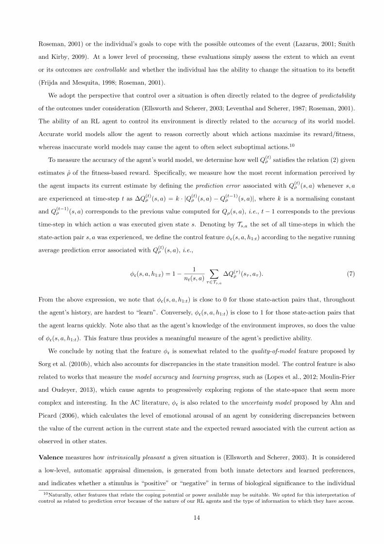
state-action pair s, a was experienced, we define the control feature φc(s, a, h1:t) according to the negative running

average prediction error associated with Q(t)ρ (s, a), i.e.,

φc(s, a, h1:t) = 1− 1

nt(s, a)

∑τ∈Ts,a

∆Q(τ)ρ (sτ , aτ ). (7)

From the above expression, we note that φc(s, a, h1:t) is close to 0 for those state-action pairs that, throughout

the agent’s history, are hardest to “learn”. Conversely, φc(s, a, h1:t) is close to 1 for those state-action pairs that

the agent learns quickly. Note also that as the agent’s knowledge of the environment improves, so does the value

of φc(s, a, h1:t). This feature thus provides a meaningful measure of the agent’s predictive ability.

We conclude by noting that the feature φc is somewhat related to the quality-of-model feature proposed by

Sorg et al. (2010b), which also accounts for discrepancies in the state transition model. The control feature is also

related to works that measure the model accuracy and learning progress, such as (Lopes et al., 2012; Moulin-Frier

and Oudeyer, 2013), which cause agents to progressively exploring regions of the state-space that seem more

complex and interesting. In the AC literature, φc is also related to the uncertainty model proposed by Ahn and

Picard (2006), which calculates the level of emotional arousal of an agent by considering discrepancies between

the value of the current action in the current state and the expected reward associated with the current action as

observed in other states.

Valence measures how intrinsically pleasant a given situation is (Ellsworth and Scherer, 2003). It is considered

a low-level, automatic appraisal dimension, is generated from both innate detectors and learned preferences,

and indicates whether a stimulus is “positive” or “negative” in terms of biological significance to the individual

10Naturally, other features that relate the coping potential or power available may be suitable. We opted for this interpretation ofcontrol as related to prediction error because of the nature of our RL agents and the type of information to which they have access.

14

(Leventhal and Scherer, 1987). Unlike the other dimensions, valence is considered a feature of the stimulus itself

and is mostly independent of the momentary situation of the individual (Ellsworth and Scherer, 2003).

At such a low level, in our IMRL framework, valence is perhaps best represented as the fitness-based reward

itself, φρ, because it provides an immediate direct evaluation of the perceived states and executed actions in terms

of the associated fitness. However, as observed in Section 3.2, φρ is external to the agent and fails to take into

account any experience that the agent may accumulate. Alternatively, we adopt the idea that the implicit value

of things can change throughout time according to experience (Cardinal et al., 2002; Ellsworth and Scherer, 2003;

Leventhal and Scherer, 1987). Bearing this idea in mind, and to account for the integration of experience in the

valence dimension of appraisal, we evaluate the value of the agent’s current situation (with respect to fitness),

both in terms of the perceived state and in terms of the experienced action.

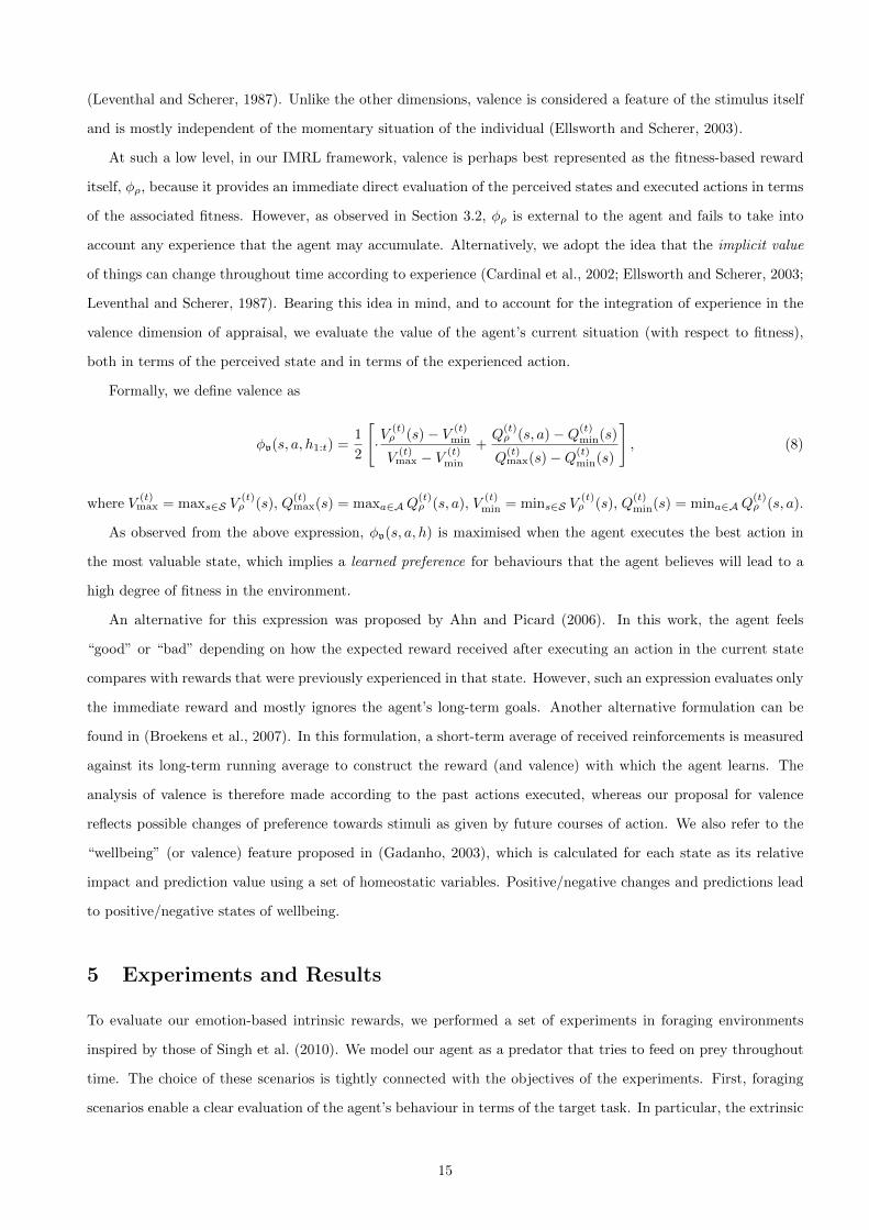
Formally, we define valence as

φv(s, a, h1:t) =1

2

[·V

(t)ρ (s)− V (t)

min

V(t)max − V (t)

min

+Q

(t)ρ (s, a)−Q(t)

min(s)

Q(t)max(s)−Q(t)

min(s)

], (8)

where V(t)max = maxs∈S V

(t)ρ (s), Q

(t)max(s) = maxa∈AQ

(t)ρ (s, a), V

(t)min = mins∈S V

(t)ρ (s), Q

(t)min(s) = mina∈AQ

(t)ρ (s, a).

As observed from the above expression, φv(s, a, h) is maximised when the agent executes the best action in

the most valuable state, which implies a learned preference for behaviours that the agent believes will lead to a

high degree of fitness in the environment.

An alternative for this expression was proposed by Ahn and Picard (2006). In this work, the agent feels

“good” or “bad” depending on how the expected reward received after executing an action in the current state

compares with rewards that were previously experienced in that state. However, such an expression evaluates only

the immediate reward and mostly ignores the agent’s long-term goals. Another alternative formulation can be

found in (Broekens et al., 2007). In this formulation, a short-term average of received reinforcements is measured

against its long-term running average to construct the reward (and valence) with which the agent learns. The

analysis of valence is therefore made according to the past actions executed, whereas our proposal for valence

reflects possible changes of preference towards stimuli as given by future courses of action. We also refer to the

“wellbeing” (or valence) feature proposed in (Gadanho, 2003), which is calculated for each state as its relative

impact and prediction value using a set of homeostatic variables. Positive/negative changes and predictions lead

to positive/negative states of wellbeing.

5 Experiments and Results

To evaluate our emotion-based intrinsic rewards, we performed a set of experiments in foraging environments

inspired by those of Singh et al. (2010). We model our agent as a predator that tries to feed on prey throughout

time. The choice of these scenarios is tightly connected with the objectives of the experiments. First, foraging

scenarios enable a clear evaluation of the agent’s behaviour in terms of the target task. In particular, the extrinsic

15

(a) Hungry-Thirsty (b) Lairs (c) Moving-Prey (d) Persistence (e) “Seasons”

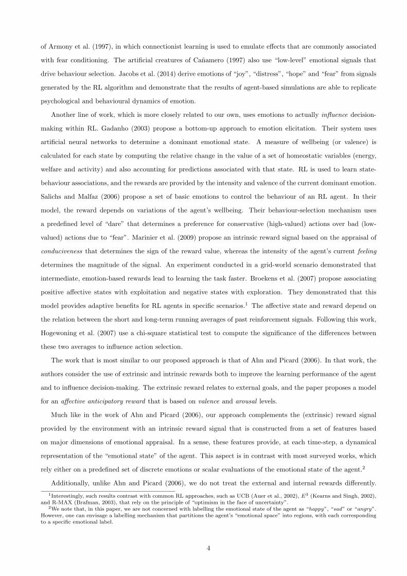
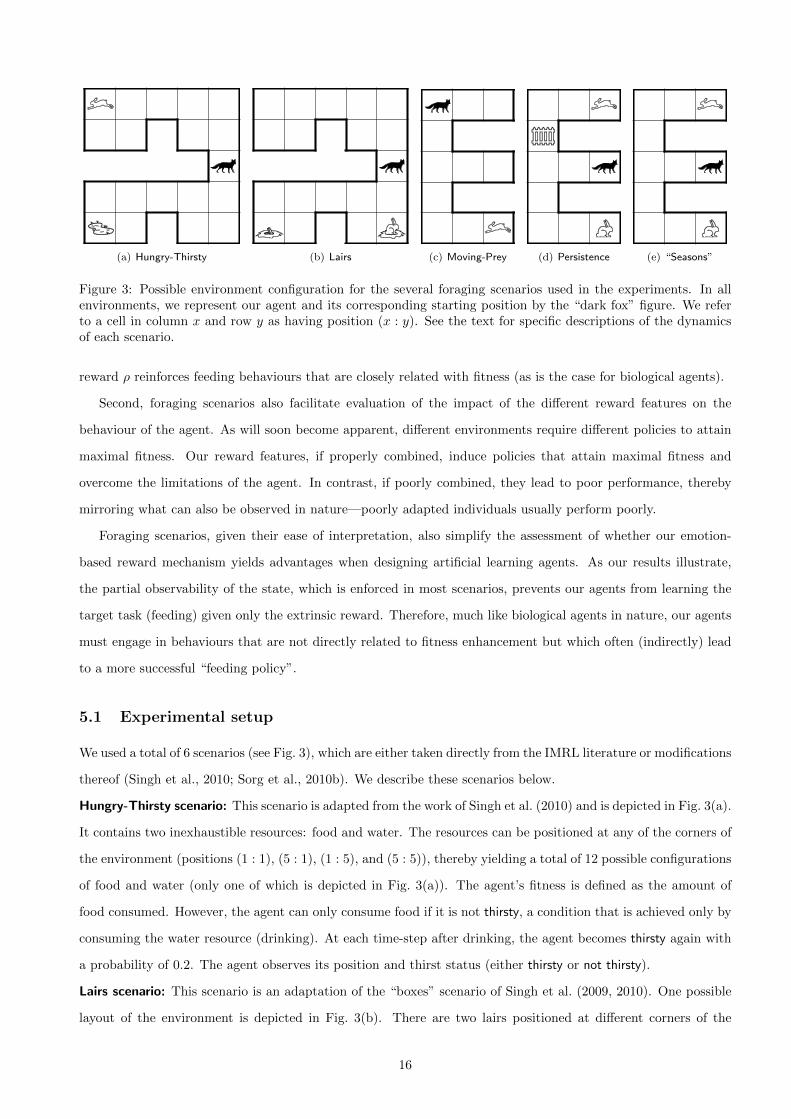
Figure 3: Possible environment configuration for the several foraging scenarios used in the experiments. In allenvironments, we represent our agent and its corresponding starting position by the “dark fox” figure. We referto a cell in column x and row y as having position (x : y). See the text for specific descriptions of the dynamicsof each scenario.

reward ρ reinforces feeding behaviours that are closely related with fitness (as is the case for biological agents).

Second, foraging scenarios also facilitate evaluation of the impact of the different reward features on the

behaviour of the agent. As will soon become apparent, different environments require different policies to attain

maximal fitness. Our reward features, if properly combined, induce policies that attain maximal fitness and

overcome the limitations of the agent. In contrast, if poorly combined, they lead to poor performance, thereby

mirroring what can also be observed in nature—poorly adapted individuals usually perform poorly.

Foraging scenarios, given their ease of interpretation, also simplify the assessment of whether our emotion-

based reward mechanism yields advantages when designing artificial learning agents. As our results illustrate,

the partial observability of the state, which is enforced in most scenarios, prevents our agents from learning the

target task (feeding) given only the extrinsic reward. Therefore, much like biological agents in nature, our agents

must engage in behaviours that are not directly related to fitness enhancement but which often (indirectly) lead

to a more successful “feeding policy”.

5.1 Experimental setup

We used a total of 6 scenarios (see Fig. 3), which are either taken directly from the IMRL literature or modifications

thereof (Singh et al., 2010; Sorg et al., 2010b). We describe these scenarios below.

Hungry-Thirsty scenario: This scenario is adapted from the work of Singh et al. (2010) and is depicted in Fig. 3(a).

It contains two inexhaustible resources: food and water. The resources can be positioned at any of the corners of

the environment (positions (1 : 1), (5 : 1), (1 : 5), and (5 : 5)), thereby yielding a total of 12 possible configurations

of food and water (only one of which is depicted in Fig. 3(a)). The agent’s fitness is defined as the amount of

food consumed. However, the agent can only consume food if it is not thirsty, a condition that is achieved only by

consuming the water resource (drinking). At each time-step after drinking, the agent becomes thirsty again with

a probability of 0.2. The agent observes its position and thirst status (either thirsty or not thirsty).

Lairs scenario: This scenario is an adaptation of the “boxes” scenario of Singh et al. (2009, 2010). One possible

layout of the environment is depicted in Fig. 3(b). There are two lairs positioned at different corners of the

16

environment, thereby resulting in 6 possible configurations. The fitness of the agent is defined as the number of

prey captured. Whenever a lair is occupied by a prey, the agent can drive the prey out by means of a Pull action.

The state of the lair transitions to prey outside, and the agent has exactly one time-step to capture the prey with

a Capture action before the prey runs away. In either case, the state of the lair transitions to empty. At every

time-step, there is a probability of 0.1 that a prey will appear in an empty lair. The agent is able to observe its

position and the state of both lairs (occupied, empty, or prey outside).

Moving-Prey scenario: This scenario is also adapted from the work of Singh et al. (2010), and one possible

configuration is depicted in Fig. 3(c). In this scenario, at any time-step, there is exactly one prey available, and

the prey is located at one of the end-of-corridor locations (positions (3 : 1), (3 : 3) or (3 : 5)). The agent’s fitness

is again defined as the number of prey captured. Whenever the agent captures a prey, the latter disappears from

the current location and a new prey randomly appears at one of the two other possible prey locations.

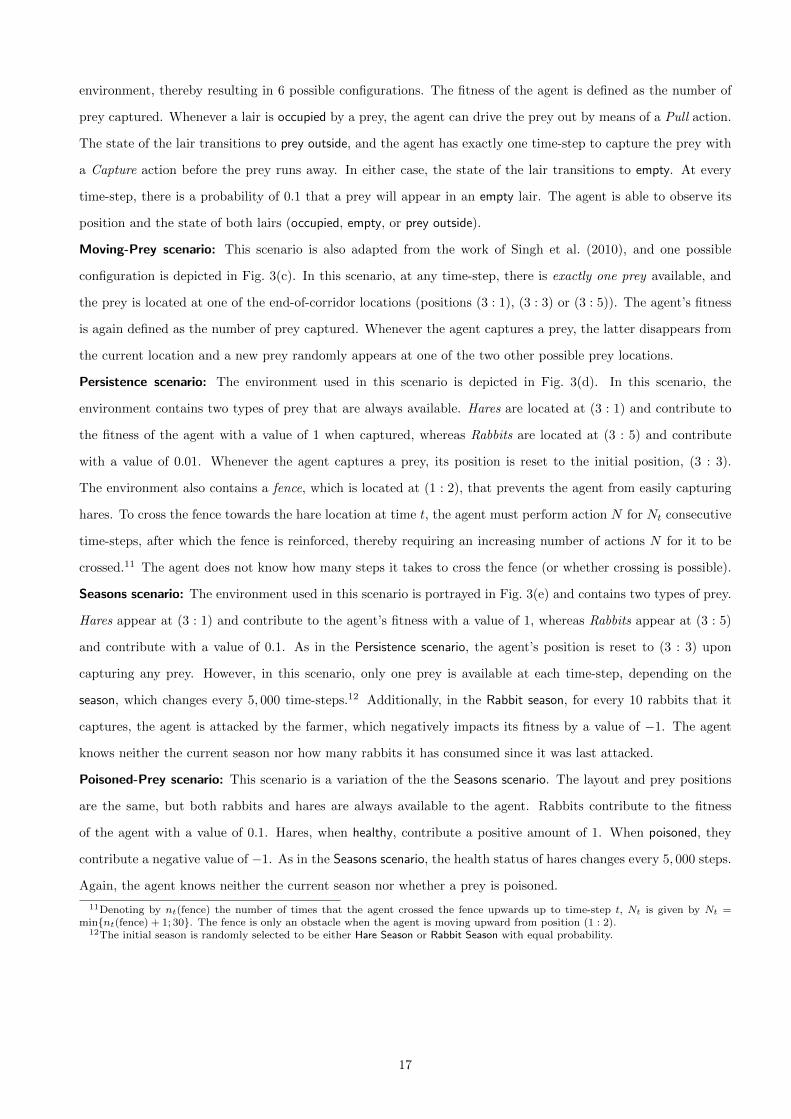
Persistence scenario: The environment used in this scenario is depicted in Fig. 3(d). In this scenario, the

environment contains two types of prey that are always available. Hares are located at (3 : 1) and contribute to

the fitness of the agent with a value of 1 when captured, whereas Rabbits are located at (3 : 5) and contribute

with a value of 0.01. Whenever the agent captures a prey, its position is reset to the initial position, (3 : 3).

The environment also contains a fence, which is located at (1 : 2), that prevents the agent from easily capturing

hares. To cross the fence towards the hare location at time t, the agent must perform action N for Nt consecutive

time-steps, after which the fence is reinforced, thereby requiring an increasing number of actions N for it to be

crossed.11 The agent does not know how many steps it takes to cross the fence (or whether crossing is possible).

Seasons scenario: The environment used in this scenario is portrayed in Fig. 3(e) and contains two types of prey.

Hares appear at (3 : 1) and contribute to the agent’s fitness with a value of 1, whereas Rabbits appear at (3 : 5)

and contribute with a value of 0.1. As in the Persistence scenario, the agent’s position is reset to (3 : 3) upon

capturing any prey. However, in this scenario, only one prey is available at each time-step, depending on the

season, which changes every 5, 000 time-steps.12 Additionally, in the Rabbit season, for every 10 rabbits that it

captures, the agent is attacked by the farmer, which negatively impacts its fitness by a value of −1. The agent

knows neither the current season nor how many rabbits it has consumed since it was last attacked.

Poisoned-Prey scenario: This scenario is a variation of the the Seasons scenario. The layout and prey positions

are the same, but both rabbits and hares are always available to the agent. Rabbits contribute to the fitness

of the agent with a value of 0.1. Hares, when healthy, contribute a positive amount of 1. When poisoned, they

contribute a negative value of −1. As in the Seasons scenario, the health status of hares changes every 5, 000 steps.

Again, the agent knows neither the current season nor whether a prey is poisoned.

11Denoting by nt(fence) the number of times that the agent crossed the fence upwards up to time-step t, Nt is given by Nt =min{nt(fence) + 1; 30}. The fence is only an obstacle when the agent is moving upward from position (1 : 2).

12The initial season is randomly selected to be either Hare Season or Rabbit Season with equal probability.

17

Agent Description

In all scenarios, the agent is modelled as a POMDP whose state dynamics follow from the above descriptions.

In all scenarios, the agent has 4 available actions, A = {N,S,E,W}, that deterministically move it in the

corresponding direction. In the Lairs scenario, the agent has also Pull and Capture actions available. Prey are

captured automatically whenever they are co-located with the agent. In all but the Hungry-Thirsty and Lairs

scenarios, the agent is only able to observe its current (x : y) position and whether it is collocated with a prey.

In all scenarios, we treat observations as states and use prioritised sweeping to learn a policy that maps

observations to actions (Moore and Atkeson, 1993). As discussed in Section 3, prioritised sweeping constructs

a model of the environment and uses this model to perform value-iteration updates. Specifically, our agent

maintains an estimate P(t)(s′ | s, a) of the transition probabilities as perceived by the agent, which is given by

P(t)(s′ | s, a) = 1nt(s,a)

∑tτ=1 I(s,a,s′)(sτ , aτ , sτ+1). The reward features discussed in Section 4.3 are then used to

build the intrinsic reward and thus compute the associated optimal Q-function, Q∗. In our experiments, prioritised

sweeping updates the Q-values of up to 10 state-action pairs in each iteration using a learning rate of α = 0.3.

During its lifetime, the agent uses an ε-greedy exploration strategy with a decaying exploration parameter εt = λt,

where λ = 0.999. We use a novelty rate λn = 1.001 for the computation of the novelty reward-feature in (5). In

all experiments, we consider a discount of γ = 0.9.

Reward parameter optimization

We consider the space of rewards, R, as the set of all rewards of the form r(s, a, h) = φ(s, a, h)>θ, where φ(s, a, h)

is the set of all reward features described in Section 4.3 and θ is the vector that contains the corresponding

parameters that represent the weight or contribution of each feature to the overall reward. To determine the

optimal reward function r∗ (or, equivalently, the corresponding optimal parameter vector θ∗) for each of the

different (set of) environments considered, we adopt the simple approach of Singh et al. (2010). In particular, we

restrict the parameter vector to lie in the 5-dimensional hypercube I = [−1; 1]5 and sample a total of K = 14, 003

uniformly distributed parameter vectors from I, where we enforce ‖θk‖1 = 1, k = 1, . . . ,K.

As discussed in Section 3.2, we consider the fitness function defined in (4). To evaluate the fitness of an agent

driven by reward rk = φ>θk, k = 1, . . . ,K,, we perform a total of N = 200 independent Monte Carlo trials,

each of which consisting of a continuous run of 100, 000 learning steps. During each trial, the agent is allowed

to interact with and learn from the environment. The fitness of the agent given a reward function rk is then

measured as the average fitness across the N trials, i.e., F (rk) ≈ 1N

∑Ni=1 f(hi), where hi is the history of the

agent at trial i. Finally, we select the optimal parameter vector, θ∗, such that θ∗ = argmaxθk,k=1,...,K F(rk).

5.2 Results

We now describe the results of our experiments, which are detailed in Table 1. For each scenario, we indicate the

optimal parameter vector, θ∗, that results from the parameter optimisation procedure described in Section 5.1.

We then compare the fitness attained by our “emotion-driven” RL agent, which is driven by r∗ = φ>θ∗, with

18

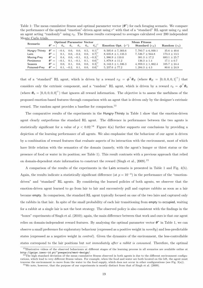
Table 1: The mean cumulative fitness and optimal parameter vector (θ∗) for each foraging scenario. We comparethe performance of the optimal “emotion”-driven agent using r∗ with that of a “standard” RL agent using rE andan agent acting “randomly” using r0. The fitness results correspond to averages calculated over 200 independentMonte Carlo trials.

ScenarioOptimal Parameter Vector Mean Fitness

θ∗ = [ θn, θr, θc, θv, θρ]> Emotion Opt. (r∗) Standard (rE) Random (r0)

Hungry-Thirsty θ∗ = [ −0.4, 0.0, 0.0, 0.5, 0.1]> 9, 505.6 ± 7, 303.6 7, 783.7 ± 6, 930.1 35.6 ± 40.6Lairs θ∗ = [ 0.1, 0.0, −0.2, 0.0, 0.7]> 8, 635.8 ± 1, 133.3 7, 536.7 ± 944.8 173.3 ± 13.5Moving-Prey θ∗ = [ 0.4, 0.0, −0.1, 0.2, −0.3]> 1, 986.9 ± 110.0 381.3 ± 17.2 683.1 ± 25.7Persistence θ∗ = [ −0.1, 0.1, −0.1, 0.1, 0.6]> 1, 879.8 ± 11.2 136.3 ± 1.4 17.1 ± 0.7Seasons θ∗ = [ 0.0, 0.1, 0.6, 0.0, 0.3]> 6, 142.3 ± 1, 336.3 4, 959.3 ± 1, 862.4 105.7 ± 24.4Poisoned-Prey θ∗ = [ 0.1, −0.2, 0.1, 0.0, 0.6]> 5, 237.6 ± 77.2 1, 284.3 ± 4.3 80.6 ± 24.9

that of a “standard” RL agent, which is driven by a reward rE = φ>θE (where θE = [0, 0, 0, 0, 1]>) that

considers only the extrinsic component, and a “random” RL agent, which is driven by a reward r0 = φ>θ0

(where θ0 = [0, 0, 0, 0, 0]>) that ignores all reward information. The objective is to assess the usefulness of the

proposed emotion-based features through comparison with an agent that is driven only by the designer’s extrinsic

reward. The random agent provides a baseline for comparison.13

The comparative results of the experiments in the Hungry-Thirsty in Table 1 show that the emotion-driven

agent clearly outperforms the standard RL agent. The difference in performance between the two agents is

statistically significant for a value of p < 0.02.14 Figure 4(a) further supports our conclusions by providing a

depiction of the learning performance of all agents. We also emphasise that the behaviour of our agent is driven

by a combination of reward features that evaluate aspects of its interaction with the environment, most of which

have little relation with the semantics of the domain (namely, with the agent’s hunger or thirst status or the

presence of food or water in its position; see Table 1). This result contrasts with a previous approach that relied

on domain-dependent state information to construct the reward (Singh et al., 2009).15

A comparison of the results of the experiments in the Lairs scenario is presented in Table 1 and Fig. 4(b).

Again, the results indicate a statistically significant difference (at p = 10−4) in the performance of the “emotion-

driven” and “standard” RL agents. By considering the learned policies of both agents, we observer that the

emotion-driven agent learned to go from lair to lair and successively pull and capture rabbits as soon as a lair

became empty. In comparison, the standard RL agent typically focused on one of the two lairs and captured only

the rabbits in that lair. In spite of the small probability of each lair transitioning from empty to occupied, waiting

for a rabbit at a single lair is not the best strategy. The observed policy is also consistent with the findings in the

“boxes” experiments of Singh et al. (2010); again, the main difference between that work and ours is that our agent

relies on domain-independent reward features. By analysing the optimal parameter vector θ∗ in Table 1, we can

observe a small preference for exploratory behaviour (expressed as a positive weight in novelty) and less-predictable

states (expressed as a negative weight in control). Given the dynamics of the environment, the less-controllable

states correspond to the lair positions but not immediately after a rabbit is consumed. Therefore, the optimal

13Illustrative videos of the observed behaviours at different stages of the learning process in all scenarios are available online athttp://gaips.inesc-id.pt/~psequeira/emot-design/.

14The high standard deviation of the mean cumulative fitness observed in both agents is due to the different environment configu-rations, which lead to very different fitness values. For example, when the food and water are both located on the left, the agent musttraverse the environment to move from the water to the food supply, which does not occur in other configurations (see Fig. 3(a)).

15We note, however, that the purpose of our experiments is mostly distinct from that of Singh et al. (2009).

19

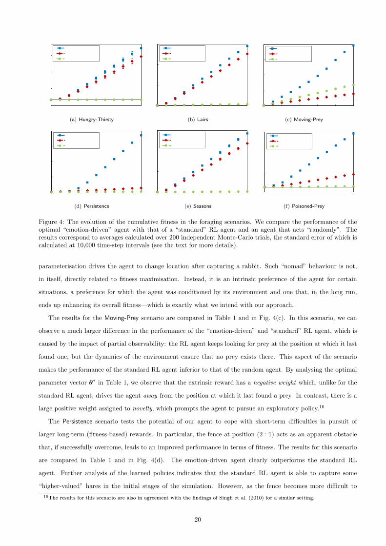
(a) Hungry-Thirsty (b) Lairs (c) Moving-Prey

(d) Persistence (e) Seasons (f) Poisoned-Prey

Figure 4: The evolution of the cumulative fitness in the foraging scenarios. We compare the performance of theoptimal “emotion-driven” agent with that of a “standard” RL agent and an agent that acts “randomly”. Theresults correspond to averages calculated over 200 independent Monte-Carlo trials, the standard error of which iscalculated at 10,000 time-step intervals (see the text for more details).

parameterisation drives the agent to change location after capturing a rabbit. Such “nomad” behaviour is not,

in itself, directly related to fitness maximisation. Instead, it is an intrinsic preference of the agent for certain

situations, a preference for which the agent was conditioned by its environment and one that, in the long run,

ends up enhancing its overall fitness—which is exactly what we intend with our approach.

The results for the Moving-Prey scenario are compared in Table 1 and in Fig. 4(c). In this scenario, we can

observe a much larger difference in the performance of the “emotion-driven” and “standard” RL agent, which is

caused by the impact of partial observability: the RL agent keeps looking for prey at the position at which it last

found one, but the dynamics of the environment ensure that no prey exists there. This aspect of the scenario

makes the performance of the standard RL agent inferior to that of the random agent. By analysing the optimal

parameter vector θ∗ in Table 1, we observe that the extrinsic reward has a negative weight which, unlike for the

standard RL agent, drives the agent away from the position at which it last found a prey. In contrast, there is a

large positive weight assigned to novelty, which prompts the agent to pursue an exploratory policy.16

The Persistence scenario tests the potential of our agent to cope with short-term difficulties in pursuit of

larger long-term (fitness-based) rewards. In particular, the fence at position (2 : 1) acts as an apparent obstacle

that, if successfully overcome, leads to an improved performance in terms of fitness. The results for this scenario

are compared in Table 1 and in Fig. 4(d). The emotion-driven agent clearly outperforms the standard RL

agent. Further analysis of the learned policies indicates that the standard RL agent is able to capture some

“higher-valued” hares in the initial stages of the simulation. However, as the fence becomes more difficult to

16The results for this scenario are also in agreement with the findings of Singh et al. (2010) for a similar setting.

20

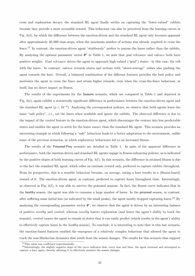
cross and exploration decays, the standard RL agent finally settles on capturing the “lower-valued” rabbits

because they provide a more accessible reward. This behaviour can also be perceived from the learning curves in

Fig. 4(d), for which the difference between the emotion-driven and the standard RL agent only becomes apparent

after approximately 20, 000 time-steps, when the maximum number of actions was already required to cross the

fence.17 In contrast, the emotion-driven agent “stubbornly” prefers to pursue the hares rather than the rabbits.

By analysing the optimal parameter vector θ∗ in Table 1, we note that goal relevance and valence both have

positive weights. Goal relevance drives the agent to approach high-valued (“goal”) states—in this case, the cell

with the hares. In contrast, valence rewards states and actions with “above-average” values also pushing the

agent towards the hare. Overall, a balanced combination of the different features provides the best policy and

motivates the agent to cross the fence and attain higher rewards, even when the cross-the-fence behaviour, in

itself, has no direct impact on fitness.

The results of the experiments for the Seasons scenario, which are compared in Table 1 and depicted in

Fig. 4(e), again exhibit a statistically significant difference in performance between the emotion-driven agent and

the standard RL agent (p < 10−4). Analysing the correspondent policies, we observe that both agents learn the

same “safe policy”, i.e., eat the hares when available and ignore the rabbits. The observed difference is due to

the impact of the control feature in the emotion-driven agent, which discourages the venture into less predictable

states and enables the agent to settle for the hares sooner than the standard RL agent. This scenario provides an

interesting example in which following a “safe” behaviour leads to a better adaptation to the environment, unlike

some of the previous scenarios, in which exploratory behaviours led to an increased fitness.

The results of the Poisoned-Prey scenario are detailed in Table 1. In spite of the apparent difference in

performance, both the emotion-driven and standard RL agents engage in fitness-enhancing policies, as is indicated

by the positive slopes of both learning curves of Fig. 4(f). In this scenario, the difference in attained fitness is due

to the fact the standard RL agent, which relies on extrinsic reward only, preferred to capture rabbits throughout.

From its perspective, this is a sensible behaviour because, on average, eating a hare results in a (fitness-based)

reward of 0. The emotion-driven agent, in contrast, preferred to capture hares throughout time. Interestingly,

as observed in Fig. 4(f), it was able to survive the poisoned seasons. In fact, the fitness curve indicates that in

the healthy season, the agent was able to consume a large number of hares. In the poisoned season, in contrast,

after suffering some initial loss (as indicated by the small peaks), the agent mostly stopped capturing hares.18 By

analysing the corresponding parameter vector θ∗, we observe that the agent is driven by an interesting balance

of positive novelty and control ; whereas novelty fosters exploration (and hence the agent’s ability to track the

seasons), control causes the agent to remain in states that it can easily predict (which results in the agent’s ability

to effectively capture hares in the healthy season). To conclude, it is interesting to note that in this last scenario,

the emotion-based features enabled the emergence of a relatively complex behaviour that allowed the agent to

track the non-Markovian dynamics that result from the season changes. The results for this scenario thus support

17This value was confirmed experimentally.18Interestingly, the slightly negative slope of the curve indicates that, every now and then, the agent returned and attempted to

capture a hare again, thereby allowing it to effectively monitor the season changes.

21

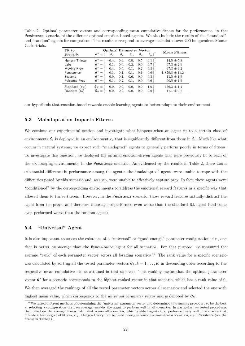
Table 2: Optimal parameter vectors and corresponding mean cumulative fitness for the performance, in thePersistence scenario, of the different optimal emotion-based agents. We also include the results of the “standard”and “random” agents for comparison. The results correspond to averages calculated over 200 independent MonteCarlo trials.

Fit to Optimal Parameter VectorMean Fitness

Scenario θ∗ = [ θn, θr, θc, θv, θρ ]>

Hungry-Thirsty θ∗ = [ −0.4, 0.0, 0.0, 0.5, 0.1 ]> 14.5 ± 5.8Lairs θ∗ = [ 0.1, 0.0, −0.2, 0.0, 0.7 ]> 67.3 ± 2.1Moving-Prey θ∗ = [ 0.4, 0.0, −0.1, 0.2, −0.3 ]> 47.3 ± 4.2Persistence θ∗ = [ −0.1, 0.1, −0.1, 0.1, 0.6 ]> 1, 879.8 ± 11.2Seasons θ∗ = [ 0.0, 0.1, 0.6, 0.0, 0.3 ]> 11.5 ± 1.5Poisoned-Prey θ∗ = [ 0.1, −0.2, 0.1, 0.0, 0.6 ]> 60.5 ± 1.5

Standard (rE) θE = [ 0.0, 0.0, 0.0, 0.0, 1.0 ]> 136.3 ± 1.4Random (r0) θ0 = [ 0.0, 0.0, 0.0, 0.0, 0.0 ]> 17.1 ± 0.7

our hypothesis that emotion-based rewards enable learning agents to better adapt to their environment.

5.3 Maladaptation Impacts Fitness

We continue our experimental section and investigate what happens when an agent fit to a certain class of

environments E1 is deployed in an environment e2 that is significantly different from those in E1. Much like what

occurs in natural systems, we expect such “maladapted” agents to generally perform poorly in terms of fitness.

To investigate this question, we deployed the optimal emotion-driven agents that were previously fit to each of

the six foraging environments, in the Persistence scenario. As evidenced by the results in Table 2, there was a

substantial difference in performance among the agents: the “maladapted” agents were unable to cope with the

difficulties posed by this scenario and, as such, were unable to effectively capture prey. In fact, these agents were

“conditioned” by the corresponding environments to address the emotional reward features in a specific way that

allowed them to thrive therein. However, in the Persistence scenario, those reward features actually distract the

agent from the preys, and therefore these agents performed even worse than the standard RL agent (and some

even performed worse than the random agent).

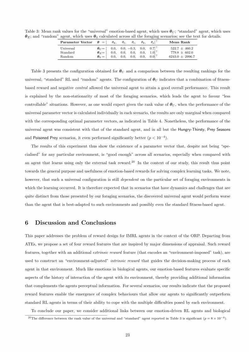
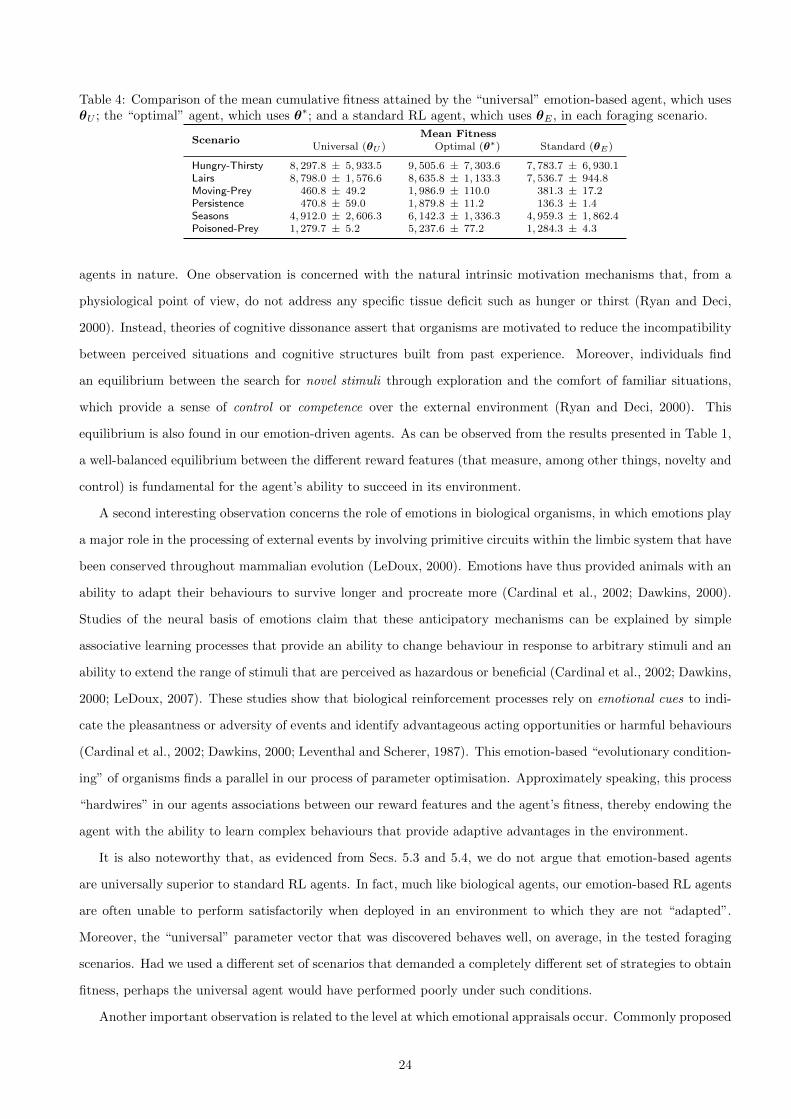
5.4 “Universal” Agent

It is also important to assess the existence of a “universal” or “good enough” parameter configuration, i.e., one

that is better on average than the fitness-based agent for all scenarios. For that purpose, we measured the

average “rank” of each parameter vector across all foraging scenarios.19 The rank value for a specific scenario

was calculated by sorting all the tested parameter vectors θk, k = 1, . . . ,K in descending order according to the

respective mean cumulative fitness attained in that scenario. This ranking means that the optimal parameter

vector θ∗ for a scenario corresponds to the highest ranked vector in that scenario, which has a rank value of 0.

We then averaged the rankings of all the tested parameter vectors across all scenarios and selected the one with

highest mean value, which corresponds to the universal parameter vector and is denoted by θU .

19We tested different methods of determining the “universal” parameter vector and determined this ranking procedure to be the bestat selecting a configuration that, on average, enables the agent to perform well in all scenarios. In particular, we tested proceduresthat relied on the average fitness calculated across all scenarios, which yielded agents that performed very well in scenarios thatprovide a high degree of fitness, e.g., Hungry-Thirsty, but behaved poorly in lower maximal-fitness scenarios, e.g., Persistence (see thefitness in Table 1).

22

Table 3: Mean rank values for the “universal” emotion-based agent, which uses θU ; “standard” agent, which usesθE ; and “random” agent, which uses θ0 calculated across all the foraging scenarios; see the text for details.

Parameter Vector θ = [ θn, θr, θc, θv, θρ]> Mean Rank

Universal θU= [ 0.0, 0.0, −0.3, 0.0, 0.7]> 522.7 ± 460.2Standard θE= [ 0.0, 0.0, 0.0, 0.0, 1.0]> 779.8 ± 602.0Random θ0 = [ 0.0, 0.0, 0.0, 0.0, 0.0]> 6243.0 ± 2996.7

Table 3 presents the configuration obtained for θU and a comparison between the resulting rankings for the

universal, “standard” RL and “random” agents. The configuration of θU indicates that a combination of fitness-

based reward and negative control allowed the universal agent to attain a good overall performance. This result

is explained by the non-stationarity of most of the foraging scenarios, which leads the agent to favour “less

controllable” situations. However, as one would expect given the rank value of θU , when the performance of the

universal parameter vector is calculated individually in each scenario, the results are only marginal when compared

with the corresponding optimal parameter vectors, as indicated in Table 4. Nonetheless, the performance of the

universal agent was consistent with that of the standard agent, and in all but the Hungry-Thirsty, Prey Seasons

and Poisoned Prey scenarios, it even performed significantly better (p < 10−4).

The results of this experiment thus show the existence of a parameter vector that, despite not being “spe-

cialised” for any particular environment, is “good enough” across all scenarios, especially when compared with

an agent that learns using only the external task reward.20 In the context of our study, this result thus point

towards the general purpose and usefulness of emotion-based rewards for solving complex learning tasks. We note,

however, that such a universal configuration is still dependent on the particular set of foraging environments in

which the learning occurred. It is therefore expected that in scenarios that have dynamics and challenges that are

quite distinct from those presented by our foraging scenarios, the discovered universal agent would perform worse

than the agent that is best-adapted to such environments and possibly even the standard fitness-based agent.

6 Discussion and Conclusions

This paper addresses the problem of reward design for IMRL agents in the context of the ORP. Departing from

ATEs, we propose a set of four reward features that are inspired by major dimensions of appraisal. Such reward

features, together with an additional extrinsic reward feature (that encodes an “environment-imposed” task), are

used to construct an “environment-adjusted” intrinsic reward that guides the decision-making process of each

agent in that environment. Much like emotions in biological agents, our emotion-based features evaluate specific

aspects of the history of interaction of the agent with its environment, thereby providing additional information

that complements the agents perceptual information. For several scenarios, our results indicate that the proposed

reward features enable the emergence of complex behaviours that allow our agents to significantly outperform

standard RL agents in terms of their ability to cope with the multiple difficulties posed by each environment.

To conclude our paper, we consider additional links between our emotion-driven RL agents and biological

20The difference between the rank value of the universal and “standard” agent reported in Table 3 is significant (p = 8× 10−4).

23

Table 4: Comparison of the mean cumulative fitness attained by the “universal” emotion-based agent, which usesθU ; the “optimal” agent, which uses θ∗; and a standard RL agent, which uses θE , in each foraging scenario.

ScenarioMean Fitness

Universal (θU ) Optimal (θ∗) Standard (θE)

Hungry-Thirsty 8, 297.8 ± 5, 933.5 9, 505.6 ± 7, 303.6 7, 783.7 ± 6, 930.1Lairs 8, 798.0 ± 1, 576.6 8, 635.8 ± 1, 133.3 7, 536.7 ± 944.8Moving-Prey 460.8 ± 49.2 1, 986.9 ± 110.0 381.3 ± 17.2Persistence 470.8 ± 59.0 1, 879.8 ± 11.2 136.3 ± 1.4Seasons 4, 912.0 ± 2, 606.3 6, 142.3 ± 1, 336.3 4, 959.3 ± 1, 862.4Poisoned-Prey 1, 279.7 ± 5.2 5, 237.6 ± 77.2 1, 284.3 ± 4.3

agents in nature. One observation is concerned with the natural intrinsic motivation mechanisms that, from a

physiological point of view, do not address any specific tissue deficit such as hunger or thirst (Ryan and Deci,

2000). Instead, theories of cognitive dissonance assert that organisms are motivated to reduce the incompatibility

between perceived situations and cognitive structures built from past experience. Moreover, individuals find

an equilibrium between the search for novel stimuli through exploration and the comfort of familiar situations,

which provide a sense of control or competence over the external environment (Ryan and Deci, 2000). This

equilibrium is also found in our emotion-driven agents. As can be observed from the results presented in Table 1,

a well-balanced equilibrium between the different reward features (that measure, among other things, novelty and

control) is fundamental for the agent’s ability to succeed in its environment.

A second interesting observation concerns the role of emotions in biological organisms, in which emotions play

a major role in the processing of external events by involving primitive circuits within the limbic system that have

been conserved throughout mammalian evolution (LeDoux, 2000). Emotions have thus provided animals with an

ability to adapt their behaviours to survive longer and procreate more (Cardinal et al., 2002; Dawkins, 2000).

Studies of the neural basis of emotions claim that these anticipatory mechanisms can be explained by simple

associative learning processes that provide an ability to change behaviour in response to arbitrary stimuli and an

ability to extend the range of stimuli that are perceived as hazardous or beneficial (Cardinal et al., 2002; Dawkins,

2000; LeDoux, 2007). These studies show that biological reinforcement processes rely on emotional cues to indi-

cate the pleasantness or adversity of events and identify advantageous acting opportunities or harmful behaviours

(Cardinal et al., 2002; Dawkins, 2000; Leventhal and Scherer, 1987). This emotion-based “evolutionary condition-

ing” of organisms finds a parallel in our process of parameter optimisation. Approximately speaking, this process

“hardwires” in our agents associations between our reward features and the agent’s fitness, thereby endowing the

agent with the ability to learn complex behaviours that provide adaptive advantages in the environment.

It is also noteworthy that, as evidenced from Secs. 5.3 and 5.4, we do not argue that emotion-based agents

are universally superior to standard RL agents. In fact, much like biological agents, our emotion-based RL agents

are often unable to perform satisfactorily when deployed in an environment to which they are not “adapted”.

Moreover, the “universal” parameter vector that was discovered behaves well, on average, in the tested foraging

scenarios. Had we used a different set of scenarios that demanded a completely different set of strategies to obtain

fitness, perhaps the universal agent would have performed poorly under such conditions.

Another important observation is related to the level at which emotional appraisals occur. Commonly proposed

24

ATEs focus on appraisals that rely on high-level cognitive concepts and mental representations (Ellsworth and

Scherer, 2003; Lazarus, 2001; Leventhal and Scherer, 1987; Scherer, 2001). However, appraisal theorists also

suggest that many appraisals, especially in the case of young children and nonhuman animals, require little

cognitive processing or even simple judgments of the event (Frijda and Mesquita, 1998; Leventhal and Scherer,

1987; Scherer, 2001). Such multilevel ATEs explain emotions as an adaptive mechanism that develops from simple,

reflex-like innate responses into more complex cognitive patterns (Leventhal and Scherer, 1987). Our emotion-

based reward features rely on rather low-level statistical “summaries” of the agent’s history of interaction with

the environment. In this multilevel perspective of appraisal, our emotion-based reward features in fact perform

low-level evaluations that are similar to those made by different appraisal dimensions. In spite of their simplicity,

however, they still allow for the individual and cross-cultural differences that are observed in human emotional

experience (see Section 4.1): our features depend both on individual characteristics of the agent, i.e., the particular

parameter vector used to construct the intrinsic reward, and on experience because the reward features are

constructed from the agent’s particular history of interaction.

In the future, we plan to extend this research to multiagent settings. In particular, we are interested in ad-

dressing the ORP in multiagent settings within IMRL. For that purpose, we intend to design domain-independent

reward features that assess the social-acceptability of behaviours to achieve cooperation between learning agents

in the context of resource-sharing scenarios.

In conclusion, we believe that the success of our approach stems from the fact that—much like the emotional

processes in biological agents—our emotion-based rewards accommodate both the specificity of the agent (its

learning algorithm and exploration policy, for example) and its environment to complement the agent’s percep-

tions. In this sense, the optimisation procedure that is required in the context of the ORP to determine the

optimal reward resembles the environmental pressures that biological organisms have been subject to throughout

evolution. And, in the case of our emotion-based rewards, just as evolution favours behaviours that seem to

enhance the fitness of the agent in the long run, the optimisation of our biologically inspired reward mechanism

enables our agents to behave, learn, and “live” much like biological organisms do.

Acknowledgments

This work was partially supported by the Portuguese Fundao para a Cincia e a Tecnologia (FCT) under project

PEst-OE/EEI/LA0021/2013.

References

Aberdeen, D. (2003). A (revised) survey of approximate methods for solving partially observable Markov decision processes.Technical report, National ICT Australia.

Ahn, H. and Picard, R. (2006). Affective cognitive learning and decision making: The role of emotions. In Proc. 18th Eur.Meeting on Cybernetics and Systems Res., pages 1–6.

Armony, J., Servan-Schreiber, D., Cohen, J., and LeDoux, J. (1997). Computational modeling of emotion: Explorationsthrough the anatomy and physiology of fear conditioning. Trends in Cognitive Sciences, 1(1):28–34.

25

Arnold, M. (1960). Emotion and Personality, volume I. Psychological Aspects. Columbia University Press.

Auer, P., Cesa-Bianchi, N., and Fischer, P. (2002). Finite-time analysis of the multiarmed bandit problem. MachineLearning, 47(2-3):235–256.

Bobrow, G. (1964). Natural language input for a computer problem solving system. PhD thesis, Massachusetts Institute ofTechnology.

Brafman, R. (2003). R-MAX: A general polynomial time algorithm for near-optimal reinforcement learning. J. MachineLearn. Res., 3:213–231.

Bratman, J., Singh, S., Lewis, R., and Sorg, J. (2012). Strong mitigation : Nesting search for good policies within searchfor good reward. In Proc. 11th Int. Joint Conf. Autonomous Agents and Multiagent Systems, pages 407–414.

Broekens, D., Kosters, W., and Verbeek, F. (2007). On affect and self-adaptation: Potential benefits of valence-controlledaction-selection. In Mira, J. and Alvarez, J., editors, Bio-inspired Modeling of Cognitive Tasks. Springer.

Canamero, D. (1997). Modeling motivations and emotions as a basis for intelligent behavior. In Proc. 1st Int. Conf.Autonomous Agents, pages 148–155.

Cardinal, R., Parkinson, J., Hall, J., and Everitt, B. (2002). Emotion and motivation: The role of the amygdala, ventralstriatum, and prefrontal cortex. Neuroscience and Biobehavioral Reviews, 26(3):321–352.

Cassandra, A. (1998). Exact and approximate algorithms for partially observable Markov decision processes. PhD thesis,Brown University.

Damasio, A. (1994). Descartes’ Error: Emotion, Reason, and the Human Brain. G.P. Putnam’s Sons.

Dawkins, M. (2000). Animal minds and animal emotions. American Zoologist, 40(6):883–888.

El-Nasr, M., Yen, J., and Ioerger, T. (2000). FLAME: Fuzzy logic adaptive model of emotions. Auton. Agents andMultiagent Systems, 3(3):219–257.

Ellsworth, P. and Scherer, K. (2003). Appraisal processes in emotion. In Davidson, R., Scherer, K., and Goldsmith, H.,editors, Handbook of the Affective Sciences. Oxford University Press.

Ernst, D., Geurts, P., and Wehenkel, L. (2005). Tree-based batch mode reinforcement learning. J. Machine Learn. Res.,6(1):503–556.

Frijda, N. and Mesquita, B. (1998). The analysis of emotions: Dimensions of variation. In Mascolo, M. and Griffin, S.,editors, What Develops in Emotional Development? Emotions, Personality, and Psychotherapy. Plenum Press.

Gadanho, S. (2003). Learning behavior-selection by emotions and cognition in a multi-goal robot task. J. Machine Learn.Res., 4(3):385–412.

Hogewoning, E., Broekens, D. J., Eggermont, J., and Bovenkamp, E. (2007). Strategies for affect-controlled action-selectionin Soar-RL. Nat. Insp. Problem-Solving Methods in Knowledge Eng., 4528:501–510.

Jaakkola, T., Singh, S., and Jordan, M. (1995). Reinforcement learning algorithm for partially observable Markov decisionproblems. In Adv. Neural Information Proc. Systems, volume 7, pages 345–352.

Jacobs, E., Broekens, J., and Jonker, C. (2014). Emergent dynamics of joy, distress, hope and fear in reinforcement learningagents. In Proc. AAMAS Workshop on Adaptive Learning Agents.

Kaelbling, L., Littman, M., and Cassandra, A. (1998). Planning and acting in partially observable stochastic domains.Artificial Intelligence, 101:99–134.

Kaelbling, L., Littman, M., and Moore, A. (1996). Reinforcement learning: A survey. J. Artificial Intelligence Res.,4:237–285.

Kearns, M. and Singh, S. (2002). Near-optimal reinforcement learning in polynomial time. Machine Learning, 49(2-3):209–232.

Lazarus, R. (2001). Relational meaning and discrete emotions. In Scherer, K., Schorr, A., and Johnstone, T., editors,Appraisal processes in emotion: Theory, methods, research, pages 37–67. Oxford University Press.

LeDoux, J. (2000). Emotion circuits in the brain. Annual Review of Neuroscience, 23(1):155–184.

LeDoux, J. (2007). The amygdala. Current Biology, 17(20):868–874.

Leventhal, H. and Scherer, K. (1987). The relationship of emotion to cognition: A functional approach to a semanticcontroversy. Cognition & Emotion, 1(1):3–28.

26

Littman, M. (1994). Memoryless policies: Theoretical limitations and practical results. In Proc. 3rd Int. Conf. Simulationof Adaptive Behavior - From Animals to Animats, pages 238–245.

Littman, M., Cassandra, A., and Kaelbling, L. (1995). Learning policies for partially observable environments: Scaling up.In Proc. 12th Int. Conf. Mach. Learn., pages 362–370.

Lopes, M., Lang, T., Toussaint, M., and yves Oudeyer, P. (2012). Exploration in model-based reinforcement learning byempirically estimating learning progress. In Pereira, F., Burges, C., Bottou, L., and Weinberger, K., editors, Advancesin Neural Information Processing Systems 25, pages 206–214. Curran Associates, Inc.

Madani, O., Hanks, S., and Condon, A. (1999). On the undecidability of probabilistic planning and infinite-horizon partiallyobservable Markov decision problems. In Proc. 16th AAAI Conf. Artificial Intelligence, pages 541–548.

Marinier, R. P., Laird, J. E., and Lewis, R. L. (2009). A computational unification of cognitive behavior and emotion.Cog. Syst. Research, 10(1):48–69.

Marsella, S., Gratch, J., and Petta, P. (2010). Computational models of emotion. In Scherer, K., Banziger, T., and Roesch,E., editors, Blueprint for Affective Computing, pages 21–44. Oxford University Press.

Mataric, M. (1994). Reward functions for accelerated learning. In Proc. 11th Int. Conf. Machine Learning, pages 157–164.

McCallum, A. (1995). Instance-based utile distinctions for reinforcement learning with hidden state. In Proc. 12th Int.Conf. Machine Learning, pages 387–395.

Melo, F., Lopes, M., and Ferreira, R. (2010). Analysis of inverse reinforcement learning with perturbed demonstrations.In Proc. 19th European Conf. Artificial Intelligence, pages 349–354.

Minsky, M. (1986). The Society of Mind. Simon & Schuster, Inc.

Moore, A. and Atkeson, C. (1993). Prioritized sweeping: Reinforcement learning with less data and less real time. MachineLearning, 13:103–130.

Moulin-Frier, C. and Oudeyer, P. (2013). Exploration strategies in developmental robotics: a unified probabilistic frame-work. In Proc. 3rd Int. Joint Conf. Development and Learning and Epigenetic Robotics, pages 1–6. IEEE.

Neu, G. and Szepesvari, C. (2009). Training parsers by inverse reinforcement learning. Machine Learning, 77:303–337.

Newell, A. and Simon, H. (1956). The logic theory machine–a complex information processing system. IRE Transactionson Information Theory, 2(3):61–79.

Ng, A., Harada, D., and Russel, S. (1999). Policy invariance under reward transformations: Theory and application toreward shaping. In Proc. 16th Int. Conf. Machine Learning, pages 278–287.

Ng, A. and Russell, S. (2000). Algorithms for inverse reinforcement learning. In Proc. 17th Int. Conf. Machine Learn.,pages 663–670.

Niekum, S., Barto, A., and Spector, L. (2010). Genetic programming for reward function search. IEEE Trans. AutonomousMental Development, 2(2):83–90.

Picard, R. (2000). Affective Computing. MIT Press.

Puterman, M. (1994). Markov Decision Processes: Discrete Stochastic Dynamic Programming. John Wiley & Sons, Inc.

Ramachandran, D. and Amir, E. (2007). Bayesian inverse reinforcement learning. In 20th Int. Joint Conf. Art. Int., pages2586–2591.

Randløv, J. and Alstrøm, P. (1998). Learning to drive a bicycle using reinforcement learning and shaping. In Proc. 15thInt. Conf. Machine Learning.

Reisenzein, R. (2009). Emotions as metarepresentational states of mind: Naturalizing the belief-desire theory of emotion.Cognitive Systems Research, 10(1):6–20.

Roseman, I. (2001). A model of appraisal in the emotion system: Integrating theory, research, and applications. In Scherer,K., Schorr, A., and Johnstone, T., editors, Appraisal Processes in Emotion: Theory, Methods, Research, pages 68–91.Oxford University Press.

Roseman, I. and Smith, C. (2001). Appraisal theory: Overview, assumptions, varieties, controversies. In Scherer, K.,Schorr, A., and Johnstone, T., editors, Appraisal Processes in Emotion: Theory, Methods, Research, pages 3–19. OxfordUniversity Press.

Ryan, R. and Deci, E. (2000). Intrinsic and extrinsic motivations: Classic definitions and new directions. ContemporaryEducational Psychology, 25(1):54–67.

27

Salichs, M. and Malfaz, M. (2006). Using emotions on autonomous agents: The role of happiness, sadness and fear. InProc. Annual Conv. Ambient Intelligence and Simulated Behavior, pages 157–164.

Scherer, K. (2001). Appraisal considered as a process of multilevel sequential checking. In Scherer, K., Schorr, A., andJohnstone, T., editors, Appraisal Processes in Emotion: Theory, Methods, Research, pages 92–120. Oxford UniversityPress.

Sequeira, P., Melo, F., and Paiva, A. (2011a). Emotion-based intrinsic motivation for reinforcement learning agents. InProc. 4th Int. Conf. Affective Computing and Intelligent Interaction, pages 326–336.

Sequeira, P., Melo, F., Prada, R., and Paiva, A. (2011b). Emerging social awareness: Exploring intrinsic motivation inmultiagent learning. In Proc. 1st Int. Joint Conf. Development and Learning and Epigenetic Robotics, volume 2, pages1–6.

Sequeira, P., Melo, F. S., and Paiva, A. (2014). Emergence of emotional appraisal signals in reinforcement learning agents.Auton. Agents and Multiagent Systems.

Simon, H. (1967). Motivational and emotional controls of cognition. Psychological Review, 74(1):29–39.

Singh, S., Jaakkola, T., and Jordan, M. (1994). Learning without state-estimation in partially observable Markoviandecision processes. In Proc. 11th Int. Conf. Machine Learning, pages 284–292.

Singh, S., Lewis, R., and Barto, A. (2009). Where do rewards come from? In Proc. Annual Conf. Cog. Science Soc., pages2601–2606.

Singh, S., Lewis, R., Barto, A., and Sorg, J. (2010). Intrinsically motivated reinforcement learning: An evolutionaryperspective. IEEE Trans. Autonomous Mental Development, 2(2):70–82.

Smith, C. and Kirby, L. (2009). Putting appraisal in context: Toward a relational model of appraisal and emotion.Cognition & Emotion, 23(7):1352–1372.

Sorg, J., Lewis, R. L., and Singh, S. P. (2010a). Reward design via online gradient ascent. In Lafferty, J., Williams, C.,Shawe-Taylor, J., Zemel, R., and Culotta, A., editors, Advances in Neural Information Processing Systems 23, pages2190–2198. Curran Associates, Inc.

Sorg, J., Singh, S., and Lewis, R. (2010b). Internal rewards mitigate agent boundedness. In 27th ICML, pages 1007–1014.

Sutton, R. and Barto, A. (1998). Reinforcement Learning: An Introduction. The MIT Press.

Watkins, C. (1989). Learning from delayed rewards. PhD thesis, King’s College, Cambridge University.

Wiewiora, E. (2003). Potential-based shaping and Q-value initialization are equivalent. J. Artificial Intelligence Res.,19:205–208.

Winograd, T. (1971). Procedures as a representation for data in a computer program for understanding natural language.Technical Report AI Tech. Rep. 235, Massachusetts Institute of Technology.

About the Authors

Pedro Sequeira is an associate researcher at the Intelligent Agents and SyntheticCharacters Group (GAIPS) / INESC-ID in Lisbon, Portugal. He has completed thePhD Program in Information Systems and Computer Engineering at the InstitutoSuperior Tecnico of the University of Lisbon. His thesis focused on building moreflexible and robust reward mechanisms for autonomous reinforcement learning (RL)agents. His interests are in the area of artificial intelligence, particularly related withautonomous and robotic agents and multi-agent systems involving RL with intrinsicmotivation and also evolutionary/adaptive mechanisms.

Francisco S. Melo is an assistant Professor at Instituto Superior Tecnico, Universityof Lisbon, and a researcher in the GAIPS group of INESC-ID. He received his PhDin Electrical and Computer Engineering at Instituto Superior Tecnico in 2007. Sincethen he held appointments in the Computer Vision Lab of the Institute for Systemsand Robotics, in Lisbon, and in the Computer Science Department of Carnegie MellonUniversity, in the U.S.A. His research addresses problems within machine learning,particularly on reinforcement learning, planning under uncertainty, multi-agent andmulti-robot systems, developmental robotics, and sensor networks.

28

Ana Paiva is a research group leader of GAIPS at INESC-ID and a Full Professorat Instituto Superior Tecnico, University of Lisbon. She is also an Adjunct Scien-tist in the Artificial Intelligence Research Institute (IIIA) from the Spanish NationalResearch Council (CSIC) in Barcelona. She is well known in the area of IntelligentAgents and Multi-agent Systems, Artificial Intelligence, Human-Robot Interactionand Affective Computing. After her PhD in the UK, she returned to Portugal whereshe created a group on intelligent agents and synthetic characters (GAIPS). Herresearch is focused on the affective elements in the interactions between users andmachines. She served as a member of numerous international conference and work-shops. She has (co)authored over 100 publications in refereed journals, conferencesand books.

29