Learning Ensembles from Bites: A Scalable and Accurate...

Journal of Machine Learning Research 5 (2004) 421-451 Submitted 3/03; Revised 11/03; Published 4/04

Learning Ensembles from Bites:A Scalable and Accurate Approach

Nitesh V. Chawla∗ [email protected]

Customer Behavior Analytics, CIBCCommerce Court East, 11th FloorToronto, ON M5L 1A2, Canada

Lawrence O. Hall [email protected]

Department of Computer Science and EngineeringUniversity of South FloridaTampa, FL 33620, USA

Kevin W. Bowyer [email protected]

Department of Computer Science and EngineeringUniversity of Notre Dame384 Fitzpatrick HallNotre Dame, IN 46556, USA

W. Philip Kegelmeyer [email protected]

Sandia National Labs, Biosystems Research DepartmentP.O. Box 969, MS 9951Livermore, CA 94551-0969, USA

Editor: Claude Sammut

Abstract

Bagging and boosting are two popular ensemble methods that typically achieve better accuracythan a single classifier. These techniques have limitations on massive data sets, because the size ofthe data set can be a bottleneck. Voting many classifiers built on small subsets of data (“pastingsmall votes”) is a promising approach for learning from massive data sets, one that can utilizethe power of boosting and bagging. We propose a framework for building hundreds or thousandsof such classifiers on small subsets of data in a distributed environment. Experiments show thisapproach is fast, accurate, and scalable.

Keywords: ensembles, bagging, boosting, diversity, distributed learning

1. Introduction

The last decade has witnessed a surge in the availability of massive data sets. These include histori-cal data of transactions from credit card companies, telephone companies, e-commerce companies,

∗. This is the author to whom correspondence should be addressed.

c©2004 Nitesh V. Chawla, Lawrence O. Hall, Kevin W. Bowyer and W. Philip Kegelmeyer.

CHAWLA ET AL.

and financial markets. The relatively new bioinformatics field has also opened the doors to ex-tremely large data sets such as the Protein Data Bank (Berman et al., 2000). The availability ofvery large databases has constantly challenged the machine learning and data mining communityto come up with fast, scalable, and accurate approaches (Provost and Kolluri, 1999; Fayyad et al.,1996). As Neal Leavitt notes (Leavitt, 2002, p. 22):

“The two most significant challenges driving changes in data mining are scalability andperformance. Organizations want data mining to become more powerful so that theycan analyze and compare multiple data sets, not just individual large data sets, as istraditionally the case.”

Very large data sets present a challenge for both humans and machine learning algorithms. Ma-chine learning algorithms can be inundated by the flood of data, and become very slow in learninga model or classifier. Moreover, along with the large amount of data available, there is also a com-pelling need for producing results accurately and fast. Efficiency and scalability are, indeed, thekey issues when designing data mining systems for very large data sets.

The machine learning community has essentially focused on two directions to deal with massivedata sets: data subsampling (Musick et al., 1993; Provost et al., 1999), and the design of parallelor distributed approaches capable of handling all the data (Chan and Stolfo, 1993; Provost andHennessy, 1996; Hall et al., 1999; Chawla et al., 2000). The subsampling approaches build onthe assumption that “we don’t really need all the data.” The KDD-2001 conference (ACM, 2001)conducted a panel on subsampling, which overall offered positive views of subsampling. However,given 100 gigabytes of data, subsampling at 10% can itself pose a challenge. Other pertinent issueswith subsampling are: What subsampling methodology to adopt? What is the right sample size? Todo any intelligent subsampling, one might need to sort through the entire data set, which could takeaway some of the efficiency advantages. Also, some of the data mining systems are concerned withidentifying interesting patterns in a large database (Hall et al., 2000; Provost and Kolluri, 1999).In such scenarios, it could be important to have enough instances of each salient case so that thelearner can identify those patterns. A lot of business analysts want to identify interesting customerpatterns in the data sets, so taking a subsample might not help in such a scenario. Dan Graham,IBM’s director of business-intelligence solutions, notes (Leavitt, 2002, p. 22), “Data mining yieldsbetter results if more data is analyzed.” While subsampling a massive data set can simplify thelearning task, it can also degrade accuracy (Perlich et al., 2003). However, one can essentially buildan ensemble of subsamples and observe an improvement in accuracy (Eschrich et al., 2002).

The second of the two approaches to handling massive data is to bypass the need for loadingthe entire data set into the memory of a single computer. Our claim is that distributed data miningcan address, to a large extent, the scalability and efficiency issues presented by massive trainingsets. The data sets can be partitioned into a size that can be efficiently managed on a group ofprocessors. Partitioning the data sets into random, disjoint partitions will not only overcome theissue of exceeding memory size, but will also lead to creating an ensemble of diverse and accurateclassifiers, each built from a disjoint partition, but the aggregate processing all of the data (Chawlaet al., 2002b,a). This can result in an improvement in performance that might not be possible bysubsampling. Chawla et al. (2002b) show that it is possible to create multiple disjoint partitions ofboth small and very large data sets, and approach classification accuracies achievable by popularensemble techniques such as bagging, which is normally an approach suited for small data sets.

422

LEARNING ENSEMBLES FROM BITES

In this paper we show that it is also possible to learn an ensemble of classifiers from each of therandom disjoint partitions of data, and combine predictions from all those classifiers to achieve highclassification accuracies; in some cases similar to or better than boosting or distributed boosting(Lazarevic and Obradovic, 2002). We utilize Breiman’s algorithms for pasting small votes: Ivoteand Rvote (Breiman, 1999). In pasting Rvotes, small random training sets are constructed fromthe data set and classifiers are learned. In pasting Ivotes, each subsequent small training set isconstructed by importance sampling based on the quality of classifiers constructed so far. That is,the misclassified cases are given a higher probability of selection than the correctly classified casesover the learning iterations. The classifiers learned are then uniformly voted for prediction. Theseapproaches are sequential in operation, although Rvoting can be easily implemented in a distributedenvironment.

We propose a distributed setting for pasting of small votes, which can also be applicable inscenarios where data is already distributed at sites, and collecting data at one location is a costlyprocedure. Our approach is essentially “divide and conquer”: we divide the training set into ndisjoint partitions, and then Rvote or Ivote on each of the disjoint subsets independently. We callour distributed approaches to pasting Ivotes and Rvotes, DIvote and DRvote respectively (Chawlaet al., 2002a).

The organization of the rest of the paper is as follows. We discuss the related work in Section 2.We present the distributed paradigm of pasting Ivotes, Rvotes, and experimental details in Sections 3to 7. We ran the distributed learning experiments on a 24-node Beowulf cluster and the ASCI BlueSupercomputer (Livermore National Laboratories), using C4.5 release 8 decision tree (Quinlan,1992) and Cascade Correlation neural network (Fahlman and Lebiere, 1990) as the base classifiers.We show that DIvote and Ivote give very comparable accuracies, while achieving significantly betterclassification accuracies than a single classifier in most cases. One major advantage of DIvote is asignificant reduction in training time as compared with Ivote. Section 7 also includes comparisonsto distributed boosting. Section 8 contains the κ plots to highlight the diversity trends of DIvoteand DRvote. Section 9 includes empirical evidence of applicability of Ivote with a stable methodof learning such as Naive Bayes classifier (Duda et al., 2001; Good, 1965). We present the mainconclusions from our work in Section 10.

2. Related Work

One popular approach towards tackling very large training sets is “divide and conquer”, which canbe set up in a distributed learning paradigm. An advantage of this approach is that the partitionsize of the learning task can be adjusted to fit the available computational resources. One caneasily imagine a divide and conquer approach in which a data set is divided across a group ofprocessors and a classifier is learned on each processor concurrently. The classifiers are transmittedto a central processor. The central processor can then process the predictions of the independentclassifiers learned. It has been shown that combining classifiers learned on random (smaller) disjointpartitions of data can achieve the classification accuracies of the popular ensemble technique ofbagging (Chawla et al., 2002b).

Domingos (1996) describes how a specific-to-general rule induction system (RISE) was spedup by applying it to disjoint training sets. This allowed the time required for learning to becomelinear in the number of examples. The resulting rule based classifiers were voted (with weighting)in an approach similar to bagging. The major difference was that the size of each training data set

423

CHAWLA ET AL.

was much smaller than the original. On a set of 7 data sets from the UCI repository using disjointpartitions of between 100 and 500 examples, they found that the resulting classification accuracywas generally as good or better than applying RISE to all the data.

Street and Kim (2001) built an ensemble of classifiers from training data treated as a stream.Each classifier is trained on a fixed amount of data from the stream. The size of the ensemble isfixed at 25 classifiers. Classifiers “compete” for entry into the ensemble based on accuracy anddiversity. This approach allows an ensemble of classifiers to be built from an unlimited amountof training data. It also facilitates the building of an ensemble of classifiers on data with temporaldependencies, where the concept to be modeled may vary over time. In their experiments the en-semble of classifiers was usually slightly less accurate than a single classifier built with as muchdata as the current ensemble used.

Chawla et al. (2000) studied various partition strategies and found that an intelligent partitioningmethodology — clustering — is generally better than simple random partitioning, and generallyresults in a classification accuracy comparable to learning a single C4.5 tree on the entire dataset. They also found that applying bagging to the disjoint partitions, and making an ensemble ofmany C4.5 decision trees on each partition, can yield better results than building a decision tree byapplying C4.5 on the entire data set.

Bagging, boosting, and their variants have been shown to improve classifier accuracy (Freundand Schapire, 1996; Breiman, 1996; Bauer and Kohavi, 1999; Dietterich, 2000; Latinne et al., 2001).According to Breiman, bagging exploits the instability in the classifiers, since perturbing the trainingset produces different classifiers using the same algorithm. However, creating 30 or more bags of100% size can be problematic for massive data sets (Chawla et al., 2002b). We observed that fordata sets too large to handle practically in the memory of a typical computer, a committee createdusing disjoint partitions can be expected to outperform a committee created using the same numberand size of bootstrap aggregates (“bags”). Also, the performance of the committee of classifiers canbe expected to exceed that of a single classifier built from all the data (Chawla et al., 2002b).

Latinne et al. (2001) proposed a combination of bagging and random feature subsets: “Bagfs”.They generated bootstrap replicates (B) of a given training set, and for each such bag they randomlychose features without replacement F times, resulting in F feature subsets. Thus, they had B×Fnew learning sets. Using the McNemar test of significance they found that Bagfs never performedworse than bagging and Multiple Feature Subsets (MFS).

Boosting (Freund and Schapire, 1996) also creates an ensemble of classifiers from a single dataset by utilizing different training set representations of the same data set, focusing on misclassifiedcases. Boosting is essentially a sequential procedure applicable to data sets small enough to fit ina computer’s memory. Lazarevic and Obradovic (2002) proposed a distributed boosting algorithmto deal with massive data sets or very large distributed homogeneous data sets. In their framework,classifiers are learned on each distributed site, and broadcast to every other site. The ensemble ofclassifiers constructed at each site is used to compute the hypothesis, h j,t , at the jth site at iterationt. In addition, each site also broadcasts a vector with a sum of local weights, reflecting its predictionaccuracy. Each site j maintains the local distribution ∆ j,t and local weights w j,t . They try to emulatethe global distribution Dt by communicating the sums of weights from each site. Each site alsomaintains a local copy, D j,t , of the global distribution Dt , and its local distribution ∆ j, for eachboosting iteration t. The training set at site j, for each boosting iteration, is sampled accordingto D j,t . At the end of all boosting iterations, hypotheses h j,t from different sites are combinedinto a final hypothesis h f n. They achieved the same or slightly better prediction accuracy than

424


standard boosting, and they also observed a reduction in the costs of learning and the memoryrequirements for their data sets (Lazarevic and Obradovic, 2002). In Section 7, we compare DIvotewith distributed boosting.

3. Pasting Votes

Breiman (1999) proposed pasting votes to build many classifiers from small training sets or “bites”of data. He proposed two strategies of pasting votes: Ivote and Rvote. In Ivote, the small trainingset (bite) of each subsequent classifier relies on the combined hypothesis of the previous classifiers,and the sampling is done with replacement. The sampling probabilities rely on the out-of-bag error,that is, a classifier is only tested on the instances not belonging to its training set. This out-of-bag estimation gives good estimates of the generalization error (Breiman, 1999), and is used todetermine the number of iterations in the pasting votes procedure. Ivote is, thus, very similar toboosting, but the “bites” are much smaller in size than the original data set. Thus, Ivote sequentiallygenerates training sets (and thus classifiers) by importance sampling.

Rvote creates many random bites, and is a fast and simple approach. Breiman found that Rvotewas not competitive in accuracy to Ivote or Adaboost. The detailed algorithms behind both theapproaches are presented in Section 4 as part of DIvote and DRvote.

Using CART, Breiman found that pasting Ivotes gave an accuracy comparable to running Ad-aboost on the whole data set (Breiman, 1999). Pasting Ivotes does not require the entire data setto be in memory for learning; instances are drawn from the pool of training data to form muchsmaller training sets. However, sampling from the pool of training data can entail multiple randomdisk accesses, which could swamp the CPU times. So Breiman proposed an alternate scheme: asequential pass through the data set. In this scheme, an instance is read and checked to see if it willmake the training set for the next classifier in the aggregate. This is repeated in a sequential fashionuntil all N instances (size of a bite) are accumulated. The terminating condition for the algorithm isa specified number of trees or epochs, where an epoch is one sequential scan through the entire dataset. However, the sequential pass through the data set approach led to a degradation in accuracyfor a majority of the data sets. Breiman also pointed out that this approach of sequentially readinginstances from the disk will not work for highly skewed data sets. Thus, one important componentof the power of pasting Ivotes is random sampling with replacement.

The memory requirement to keep track of which instance belongs in which small training setand the number of times the instance was given a particular class is 2JNB bytes, where J is thenumber of classes and NB is the number of instances in the entire data set. Let us assume we have adata set of 108 records(NB), 1000 features (equivalent to 4 bytes each), the training set of size 105,and J = 2 (Breiman, 1999). The memory requirement will be close to a gigabyte, as follows:

A = 2∗ J ∗NB = 2∗2∗108 = 0.4 gigabytes;

B = 1000 features at 4 bytes each for 105records

= 1000∗4∗105 = 0.4 gigabytes;

C = memory required by trees stored in memory in megabytes.

Total = A+B+C ≈ 1 gigabytes.

425

CHAWLA ET AL.

In our distributed approach to pasting small votes, we divide a data set into T disjoint subsets,and assign each disjoint subset to a different processor. On each of the disjoint partitions, we followBreiman’s approach of pasting small votes. We randomly sample with replacement, as we can loadthe entire disjoint subset of data in a processor’s memory. Thus, the number of disjoint partitionscan be dictated by the amount of memory available on each processor. We combine the predictionsof all the classifiers by majority vote. Again, using the above framework of memory requirement, ifwe break up the data set into T disjoint subsets, the memory requirement will decrease by a factorof 1/T , which is substantial. So, DIvote can be more scalable than Ivote in memory. One canessentially divide a data set into subsets easily managed by the computer’s main memory.

4. Pasting DIvotes and DRvotes

The procedure for DIvote is as follows:

1. Divide the data set into T disjoint subsets.

2. Assign each disjoint subset to a unique processor.

3. On each processor build the first bite of size N by sampling with replacement from its subset,and learn a classifier.

4. Compute the out-of-bag error, e(k), and the probability of selection, c(k), as follows (Breiman,1999):

e(k) = p× e(k−1)+(1− p)× r(k).

p = 0.75. We used the same p value as used by Breiman.

k = number of classifiers in the aggregate or ensemble so far.

r(k) = error rate of the kth aggregated classifiers on a T disjoint subset.

c(k) = e(k)/(1− e(k)), probability of selecting a correctly classified instance.

5. For the subsequent bites on each of the processors, an instance is drawn at random from theresident subset of data. If this instance is misclassified by a majority vote of the out-of-bagclassifiers (those classifiers for which the instance was not in the training set), then it is put inthe subsequent bite. Otherwise, put this instance in the bite with a probability of c(k). Repeatuntil N instances have been selected for the bite (Breiman, 1999).

6. Learn the (k +1)th classifier on the bite created by step 5.

7. Repeat steps 4 to 6, until the out-of-bag error estimate plateaus, or for a given number ofiterations, to produce a desired number of classifiers. We ran our experiments for a givennumber of iterations.

8. After the desired number of classifiers have been learned, combine their predictions on thetest data using a voting mechanism. We used simple majority voting.

Pasting DRvotes follows a procedure similar to DIvotes. The only difference is that each biteis a bootstrap replicate of size N. Each instance through all iterations has the same probability of

426


being selected. DRvote is very fast, as the intermediate steps of DIvote — steps 4 and 5 in theabove algorithm — are not required. However, DRvote does not provide the accuracies achieved byDIvote. This agrees with Breiman’s observations on Rvote and Ivote.

Pasting DIvotes or DRvotes has the advantage of not requiring any communication betweenthe processors, unlike the distributed boosting approach by Lazarevic and Obradovic (2002). Thus,there is no time lost in communication among processors, as trees are built independently on eachprocessor. Furthermore, dividing the data set into smaller disjoint subsets can also mitigate the needfor larger memories. Also, if the disjoint subset size is small compared to the main memory on acomputer, the entire data set can be loaded in the memory. This will speed up the sampling fromthe data sets. Lastly, DIvote reduces the data set size on each processor, hence less examples mustbe tested by the aggregate classifiers during training, which also reduces the computational time.

5. Experimental Setup

We evaluated DIvote and DRvote by experiments on six small to moderate sized data sets, and twolarge data sets. We performed 10-fold cross-validation for almost all of our data sets, and used two-tailed paired-t-tests at the 95% confidence level to evaluate statistical significance of our results,where applicable. We also provide error bars (accuracy +/- standard error) for the Ivote, DIVote,Rvote, and DRvote in the plots. The y-axis in the plots indicates the accuracy, and the x-axisindicates the number of iterations. Please note that the number of iterations does not necessarilyequate to number of classifiers. For the distributed approaches, there are n*iterations classifiers,where n is the number of disjoint partitions. For the sequential approaches, the number of iterationsis equal to the number of classifiers in the ensemble.

5.1 Data Sets

The size of these data sets is summarized in Table 1. DNA, satimage, LED, pendigits, letter,waveform and covtype are available from the UCI repository. We used three of the four Statlog(D. Michie and Taylor, 1994) project data sets — DNA, satimage, and letter — used by Breiman(1999). We did not use the shuttle data set, as 10-fold cross-validation with C4.5 already givesaccuracies of around 99.5%, and any improvement on it will be miniscule. Moreover, we havepreviously observed that simple disjoint partitioning is able to achieve that accuracy (Chawla et al.,2000). We used a subset of 60 features (features 61 — 120) for the DNA data set (D. Michie andTaylor, 1994).

We procured the training and testing set partitions of waveform, LED and covtype from Lazare-vic and Obradovic (2002) to allow direct comparisons. One of our large data sets comes from theproblem of predicting the secondary structure of proteins (Jones, 1999). The “train and test setone” were used in developing and validating, respectively, a neural network that won the CASP-3(Livermore National Laboratories, 1999) secondary structure prediction contest. The Protein dataset (called the “Jones data set” in the rest of the paper) contains 209,529 elements in the training setand 17,731 elements in the testing set. Each amino acid in a protein can have its structure labeledas helix (H), coil (C), or sheet (E). The features for a given amino acid are twenty values in therange -17 to 17, representing the log-likelihood of the amino acid being any one of twenty basicamino acids. Using a window of size 15 centered around the target amino acid, and an extra bitper amino acid to signify where the window spans either the N or C terminus of the protein chain,gives a feature vector of size 315 (Jones, 1999). The testing set is specially constructed to avoid

427

CHAWLA ET AL.

Data Set Data Set Size Classes Number of Attributes

DNA 3,186 3 60Satimage 6,435 6 36LED Training = 6,000; Testing = 4,000 10 7Pendigits 10,992 10 16Letter 20,000 26 16Waveform Training = 40,000; Testing = 10,000 3 21Covtype Training = 149,982; Testing = 431,030 7 21Jones Training = 209,529; Testing = 17,731 3 315

Table 1: Data set sizes, number of classes, and attributes.

any homology to the training set; this makes it a hard prediction problem for the classifier, and anappropriate test for the new protein secondary structure predictions.

We performed 10-fold cross-validation for seven of our data sets: DNA, satimage, pendigits,letter, waveform, LED, and the Jones data set. For the waveform and LED data sets, we combinedthe training and testing sets to perform 10-fold cross-validation. We combined the training andtesting sets to increase the overall data set size for the learning procedures. For the Jones data setthe 10-folds were constructed per-chain from the training set, so that non-homogenity is maintainedbetween our 10-fold training and testing sets. This maintained the level of difficulty for the learningalgorithm. For the other large data set, covtype, we only ran on the separate training and testingsets of sizes 149,982 and 431,030, respectively, as done by Lazarevic and Obradovic (2002). Thesize of the entire covtype data set was too large (581,102) to perform a 10-fold cross-validation in areasonable time, given the number of approaches and classifiers.

5.2 Base Classifiers and Computing Systems

We used the C4.5 release 8 decision tree, the Cascade Correlation neural network, and Naive Bayesclassifiers for our experiments. The sequential Rvote and Ivote experiments were run on a 1.4 GHzPentium 4 Linux workstation with two gigabytes of memory, and an 8-processor Sun-Fire-880 with32 gigabytes of main memory. We ran most of our DIvote and DRvote experiments on a 24-nodeBeowulf cluster. Each node on the cluster has a 900 MHz Athlon processor and 512 megabytes ofmemory. The cluster is connected with 100Bt ethernet. We also ran some of our DIvote experimentson the ASCI Blue Supercomputer. There are 1296 compute nodes on the ASCI Blue. The 4-CPUnodes have: 1.5 gigabyte memory, 332 MHz PowerPC 604e chip, 83 Mhz memory bus, and acompute node peak performance of 2.6 GFLOP/s (Livermore National Laboratories).

6. Experiments with the C4.5 Decision Tree Learning Algorithm

We ran 10-fold cross-validation experiments using C4.5 decision trees for all the small and moderatesized data sets. Section 6.1 contains the results on the small and moderate data sets. For the largedata sets, we used separate training and testing splits. However, for one of the large data sets–Jones–we also report the 10-fold cross-validation result. Section 6.2 contains the results on the large datasets. We also present a timing analysis and comparison between DIvote and Ivote in Section 6.3.

428


0 50 100 150 200 250 30091

92

93

94

95

96

97DNA: 10−fold with C4.5

# iterations

Acc

urac

y %

DIvoteIvoteRvoteDRvoteSingle DT

Acc. +− Std. Error for DIvote Acc. +− Std. Error for Ivote

Acc. +− Std. Error for DRvote

Acc. +− Std. Error for Rvote

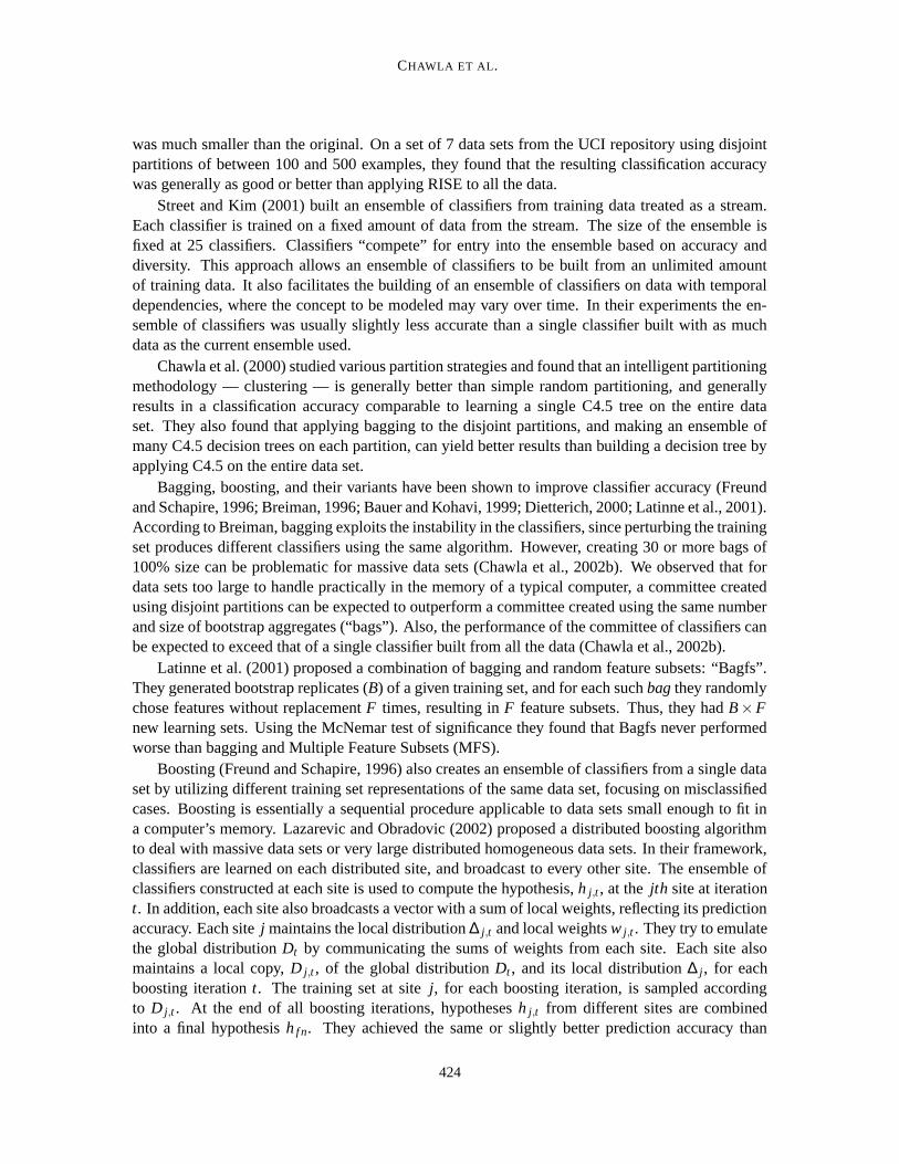
Figure 1: C4.5 Accuracy comparisons for DIvote, Ivote, DRvote, and Rvote for DNA.

6.1 Small and Moderate Sized Data Sets

We partitioned our small and moderate sized data sets, with the exception of DNA, into four disjointpartitions and used bites of size 800 to learn classifiers. Due to the smaller size of DNA, we parti-tioned it into three disjoint partitions and used bites of size 400. We used unpruned trees for all de-cision tree experiments as the ensemble of classifiers will override the overfitting (Breiman, 1999).Figures 1 to 5 show the 10-fold accuracy trends for six of our data sets. Each of the distributedapproaches is comparable in its classification accuracy to its sequential counterpart. DIvote/Ivoteachieve significantly higher classification accuracies than a single C4.5 classifier, and the simplisticapproaches of DRvote/Rvote. LED is an exception, as all the approaches are comparable to eachother. We believe that DIVote/IVote could be a victim of the feature noise present in the LED dataset, as each feature has a 10% probability of having its value inverted (Blake and Merz, 1998).

The letter data set differed from other data sets as both DRvote and Rvote achieved significantlyworse classification accuracies than C4.5. However, for letter also, DIvote and Ivote were compa-rable, and significantly better than Rvote, DRvote, and C4.5, in their classification accuracies. Theletter data set has 26 classes with 16 dimensions; each 800 sized bite will contain an average of 30instances (on an average) for each class. Thus, the 30 training instances may not mimic the real dis-tribution of the data set. To test this model, we created 100% bags on each disjoint partition (Chawlaet al., 2000) of the letter data set, and found that the classification accuracy increased significantlyas compared to DRvote or Rvote, but was still not better than DIvote and Ivote. This shows that100% random bags constructed on each disjoint partition of the letter data set are introducing morecoverage, better individual classifiers, and diversity1 compared to the DRvote bites (800 instances).

1. We visit the diversity issue in Section 8.

429

CHAWLA ET AL.

0 50 100 15071

71.5

72

72.5

73

73.5

74

74.5

75

75.5

76

Acc

urac

y %

# iterations

LED: 10−fold with C4.5

DIvoteIvoteRvoteDRvoteSingle C4.5

Acc. +− Std. Error for Ivote Acc. +− Std. Error for DIvote

Acc. +− Std. Error for DRvote Acc. +− Std. Error for Ivote

Figure 2: C4.5 Accuracy comparisons for DIvote, Ivote, DRvote, and Rvote for LED.

50 100 150 200 25085

86

87

88

89

90

91

92

93

94

Acc

urac

y %

# iterations

Satimage: 10−fold with C4.5


Acc. +− Std. Error for Ivote

Acc. +− Std. Error forD Ivote Acc. +− Std. Error for DRvote


Figure 3: C4.5 Accuracy comparisons for DIvote, Ivote, DRvote, and Rvote for satimage.

Since DIvote and Ivote sample heavily from misclassified instances, after each iteration or series ofiterations they focus on potentially different instances.

The results on the small data sets are encouraging as for almost all the data sets, DIvote issimilar to Ivote in its classification accuracy, while surpassing a single C4.5 decision tree learned on

430


50 100 150 200 250 30095

95.5

96

96.5

97

97.5

98

98.5

99

99.5

100

Acc

urac

y %

# iterations

Pendigits: 10−fold with C4.5


Acc. +− Std. Error for DIvote




Figure 4: C4.5 Accuracy comparisons for DIvote, Ivote, DRvote, and Rvote for pendigits.

50 100 150 200 250

82

84

86

88

90

92

94

96

Acc

urac

y %

# iterations

Letter: 10−fold with C4.5




Acc. +− Std. Error for Drvote


Figure 5: C4.5 Accuracy comparisons of DIvote, Ivote, Rvote, DRvote, and C4.5 for letter.

431

CHAWLA ET AL.

0 50 100 15086

88

90

92

94

96

98

100

Acc

urac

y %

# iterations

Waveform: 10−fold with C4.5






Figure 6: C4.5 Accuracy comparisons for DIvote, Ivote, DRvote, and Rvote for waveform.

the entire data set. DIvote is also significantly better than DRvote. Another important observationis that for almost all the data sets, 100 iterations of DIvote or Ivote achieve close-to-maximumaccuracies, and after that the increase in accuracy is very slow compared to the addition of iterations.Given the small bite size, 100 iterations are very fast using any algorithm as the training set size isonly 800 (or 400).

6.2 Large Data Sets

Due to the distinct nature of analysis on both the large data sets, we treat them separately in thesubsequent subsections.

6.2.1 JONES DATA SET

We set up two different experiments on the Jones data set. One evaluates the DIvote, Ivote, DRvote,and Rvote approaches by learning and testing on the provided train and test sets. The other, 10-foldcross-validation experiment, was to understand and report statistical differences between DIvoteand Ivote.

We divided the training set into 24 random disjoint partitions, as we had 24 nodes of the Beowulfcluster available for this experiment. To understand the effect of bite size on DIvote for this dataset, we also set up bites at sizes 1/256 (818 instances), 1/128 (1636 instances) and 1/64 (3272instances) of the entire training set size of 209,529. Figure 7 shows the classification accuraciesof the various approaches using the given train/test split. As is evident from the figures, all thedistributed approaches more accurate than the sequential approaches.

We also observe that increasing the bite sizes has no major effect on the classification accuraciesof the ensemble. The experiment with increasing bite sizes is computationally cheap, as the bite size

432


0 50 100 150 200 250

52

54

56

58

60

62

64

66

68

70Jones dataset with C4.5

# iterations

Acc

urac

y %

Single C4.5DIvote (24); Bite size = (1/256)JonesDIvote; (24) Bite size = (1/128)JonesDIvote (24); Bite size = (1/64)JonesIvote; Bite size = (1/256)JonesRvote; Bite size = (1/256)JonesDRvote (24); Bite size = (1/256)JonesAverage of 24 Disjoint Voting

Figure 7: Accuracy comparisons of DIvote, Ivote, Rvote, DRvote, and C4.5 for the Jones data set.

remains very small (from approximately 800 to 3200). In addition, we also show the classificationaccuracy achieved by voting classifiers learned on each of the random disjoint partitions. Notethat adding a meta-layer of DIvote on the disjoint partitions provides an absolute improvementof at least 4% in accuracy. We would also like to point out the accuracy achieved by learninga single C4.5 decision tree on the entire data set: 52.2%. It is remarkable that all the ensembleapproaches, reported in the Figure 7, provide an absolute gain of at least 12% on this data set. Thenon-homologous nature of the testing set makes it a particularly hard problem for C4.5 with its axisparallel splits (Chawla et al., 2001). The decision tree overfits the training set, achieving a very highresubstitution accuracy of 96.7%. The ensemble of decision trees counters the effect of overfittingand improves generalization, which is very important for the protein domain (Eschrich et al., 2002).

It is also interesting to note that the average accuracy of a decision tree learned on bites of size1/256th of the Jones data set (for DIvote) is below 50%, and the aggregate of all the not-so-goodclassifiers gives a performance in the range of 66% to 70% for 50 or more learning iterations. Aclassifier, learned on 1/256th of the entire training set, with an accuracy of < 50% is not verysurprising when juxtaposed with the accuracy of the single classifier learned on the entire trainingset. Figure 8 shows the accuracy trends for 4800 decision trees learned in the DIvoted ensemblefor the Jones data set. These plotted accuracies are sorted in an increasing order, and are not in thesame order as the construction of bites.

To further evaluate the behavior of DIvote and Ivote for the large Jones data set, we report the10-fold averaged cross-validation results in Figures 9 and 10. As with the previous experiment, wedivided each training fold into 24 random disjoint partitions. Let us examine Figure 9 first. DIvoteachieves significantly higher classification accuracies than Ivote for 200 iterations. However, a pointof contention could be that DIvote is constructing 200*24 (4800) classifiers versus 200 classifiersfor Ivote, albeit in less time (which is an advantage in itself of DIvote). So, on the ASCI Blue

433

CHAWLA ET AL.

0 500 1000 1500 2000 2500 3000 3500 4000 4500 500038

40

42

44

46

48

50Jones data set: Decision trees sorted by accuracy, over 200 iterations for 24 partitions

Number of trees

Acc

urac

y%

DIvote

Figure 8: Individual performances on the Jones data set.

supercomputer, we let Ivote run up to 1200 iterations or six hours (per fold) of allowed compute timeon a node. We then ran 50 (1200/24) iterations of DIvote, taking only six minutes (per fold), whichmeans that we constructed only 50 decision tree classifiers on each of the 24 disjoint partitions. Thisgave us an ensemble size of 1200 (50*24), which is equivalent to Ivote. On performing a two-tailedpaired-t-test at 95% confidence interval, we find that an ensemble of 1200 classifiers of Ivote issignificantly better (in classification accuracy) than the ensemble of 1200 classifiers of DIvote.

Now, the ensemble of DIvote classifiers is really under-constructed this time, and we can stilluse the hours of compute time utilized by Ivote to construct the ensemble. For instance, considerFigure 10, if we compare 200 DIvote classifiers that took 30 minutes and 1200 (maximal possible,given the computation bottleneck) Ivote classifiers that took six hours, we observe that DIvote andIvote are comparable to each other. This highlights the significant advantage of DIvote in terms oftime spent on computation.

6.2.2 COVTYPE

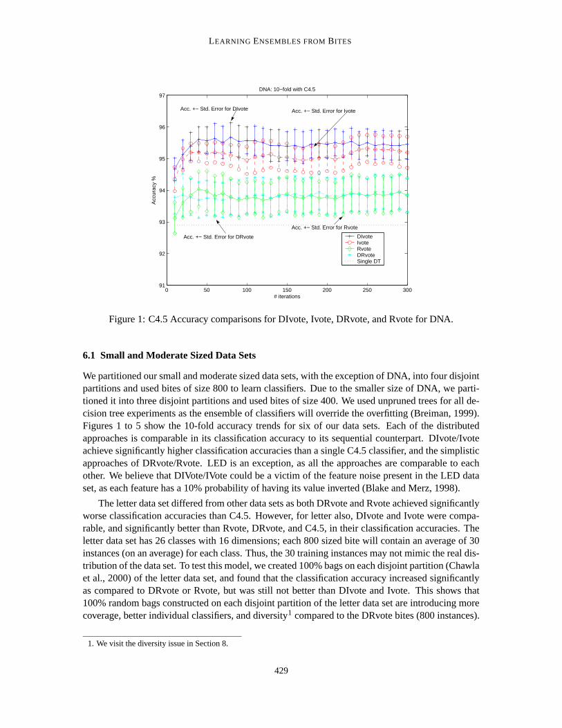
Our second large data set, covtype, contains 149,982 instances in the training set. This data set alsohas a very high skew in its class distribution as reported in Table 2. We divided the training set intoeight disjoint partitions, as done in the distributed boosting paper. We ran DIvote, Ivote, Rvote, andDRvote experiments using a bite size of 800. Figure 11 shows one of the results on this data set.Each of the ensemble approaches for covtype results in significantly worse classification accuracythan learning a single C4.5 decision tree on the entire training set. This is contrary to our previousobservations. We believe the high skew in the class distribution is coming into play, as each of theclasses is, possibly, not getting a sufficient representative coverage and interaction in the bites.

We further investigated the coverage issue by increasing the bite size for DIvote and Ivote. Asone would do in subsampling (Provost et al., 1999), we tried the following different bite sizes: 800,

434


50 100 150 2000.64

0.65

0.66

0.67

0.68

0.69

0.7

0.71

Acc

urac

y%

# iterations

Jones 10−fold with C4.5; Bite size = 800

IvoteDIvote



Figure 9: 10-fold averages of up to 200 iterations of Ivote and DIvote.

0 5 10 15 20 2564

65

66

67

68

69

70

71

Acc

urac

y

x*50 Iterations

Jones 10−fold with C4.5; Bite Size = 800

IvoteDIvote

Figure 10: 10-fold averages of up to 1200 iterations of Ivote and 200 iterations of DIvote.

435

CHAWLA ET AL.

Class 3 670Class 4 2,414Class 5 4,544Class 6 5,433Class 2 8,971Class 0 54,433Class 1 73,517

Table 2: Class distribution for the covtype data set, in ascending order.

50 100 150 200 250 30074

76

78

80

82

84

86

88

90

92

94Covtype with C4.5; Bite Size = 800

# iterations

Acc

urac

y %


Figure 11: Covtype data set with C4.5.

436


0 2000 4000 6000 8000 10000 12000 1400078

80

82

84

86

88

90

92

94

96Covtype: Varying bite sizes

Acc

urac

y %

Bite Size

DIvoteIvote

Figure 12: Effect of varying bite sizes on the covtype data set for Ivote and DIvote.

1600, 3200, 6400, 9600, 12800. We would like to point out that the bite size of 12,800 is still lessthan 10% of the training set of size 149,982. In the sequential domain, when searching for a singleappropriate subsample of a given data set, the error (or accuracy) curve at varying subsample sizesis constructed, where each (x,y) on the curve signifies the error y at a particular subsample size x.So in the ensemble setting, each (x,y) represents the voted accuracy, y, of the ensemble constructedfrom subsamples (bites) of size x. This allowed us to make an accuracy (or error) curve for theimprovement observed with varying bite sizes. Figure 12 summarizes the result. We constructed300 classifiers at each bite size. Increasing the bite size improves the coverage for the classes, andleads to a significant improvement in the prediction accuracy for both DIvote and Ivote. However,Ivote achieves higher classification accuracies than DIvote for this data set, and also surpasses theaccuracy achieved by the single C4.5 decision tree — 93.2%. The discrepancy in Ivote and DIvoteperformance is possibly arising from the limited coverage of classes in each bite from the 8 disjointpartitions; for example, each disjoint partition has, on an average, only 83 examples of class 3.

6.3 Timing

Table 3 shows the timing (user and system time during training) ratios of DIvote to Ivote, andDRvote to Rvote on the Beowulf cluster for some of our data sets using C4.5 decision trees. Wereport times for some of our small and large data sets, and with only C4.5, as the rest should followsimilar trends. The experimental parameters were: number of iterations = 100; bite size N = 800 forthe small data sets, and bite size N = (1/256) * (Jones data set size) for the Jones data set.

The time taken for DIvote and DRvote reflects the average of the time taken for 100 iterationson each of the T (T = 4 for the small data sets; T = 24 for the large data set) nodes of the cluster.For fair timing comparisons to DRvote and DIvote, we also ran 100 iterations of Ivote and Rvote ona single cluster node. It is noteworthy that we are able to build T *100 DIvote classifiers simultane-

437

CHAWLA ET AL.

Data Set DIvote/Ivote DRvote/Rvote

Satimage 0.36 0.91Pendigits 0.29 0.95Letter 0.23 0.89Jones 0.048 0.90

Table 3: Ratio of time taken by DIvote to Ivote, and DRvote to Rvote, on a cluster node.

ously. One significant advantage of the proposed DIvote approach is that it requires less time thanIvote, particularly for very large data sets. Since we divide the original training set into T disjointsubsets, during training the aggregate DIvote classifiers on a processor test many fewer instancesthan aggregate Ivote classifiers (for the Jones data set each disjoint partition has only 8730 instances,compared to 209,529 in the entire data set). Also, a reduction in the training set size implies thatthe data set can be more easily handled in main memory. This is a big gain as the multiple randomdisk accesses can then be avoided during sampling. We pointed out earlier that Breiman found thatsequential disk access was not giving as good a classification accuracy as multiple random diskaccess. So, to maintain the advantage of random sampling, each processor can load the relativelysmaller training set partition into its main memory. Table 3 shows that as the overall training dataset size increases, the ratio of DIvote time to Ivote time decreases. That is, Ivote becomes morecomputationally expensive than DIvote as the data set increases.

It is not surprising that the timings for DRvote and Rvote are very similar, as both the approachesessentially build many small bags from a given training set, without the intermediate book-keeping.Nevertheless, DRvote builds T times as many Rvote classifiers in less time.

We would like to note that the same software performs DIvote and Ivote, except that for thedistributed runs we wrote an MPI program to load our pasting votes software on different nodes ofthe cluster, and collect results. So, any further improvement of the software would be applicableacross the board, although it might decrease the ratios of time taken by DIvote to time taken byIvote. Nonetheless, it is fair to assume that Ivote will hit a memory bottleneck (with an increasingdata set size) faster than DIvote irrespective of the implementation.

7. Experiments with the Cascade Correlation Neural Network

To investigate whether our results generalize to other sorts of classifiers, we performed 10-foldcross-validation experiments on the small to moderate sized data sets using the Cascade Correla-tion (CC) neural network. We also compared the DIvote approach with the distributed boostingalgorithm, which is presented in Section 7.2.

7.1 10-fold Cross-Validation Experiments

Figures 13 to 18 summarize the results of 10-fold cross-validation with CC. Using two-tailed paired-t-tests at the 95% confidence interval, we find that DIvote and Ivote are significantly better thanDRvote, Rvote for satimage, letter, waveform, and pendigits, and comparable for DNA. DIvote andIVote are significantly better than a single CC for DNA, satimage, letter, waveform, and pendigits.DIvote and Ivote achieve comparable accuracies (no significant difference) for all the data sets,

438


0 50 100 150 200 250 30092

92.5

93

93.5

94

94.5

95

95.5

96

96.5

97DNA: 10−fold with C4.5

# iterations

Acc

urac

y %

DIvoteIvoteRvoteDRvoteSingle CC

Acc. +− Std. Error for DIVote Acc. +− Std. Error for IVote

Acc. +− Std. Error for DRVote Acc. +− Std. Error for RVote

Figure 13: CC Accuracy comparisons for DIvote, Ivote, DRvote, and Rvote for DNA.

but for pendigits. DIvote is significantly better than Ivote for pendigits. LED, again, provides anexception: all approaches are similar to each other in their classification accuracies.

We required fewer learning iterations with CC than with C4.5. Moreover, we observe that withCC, 40 to 50 iterations are sufficient, and the accuracy increases very slowly, if at all, thereafter.This is noteworthy as although neural networks are slower to learn when compared to decisiontrees, they require even fewer learning iterations. Essentially, an important conclusion to be drawnfrom all these experiments is that using importance sampling not only mitigates the need for manyiterations but also limits the amount of data needed for learning.

7.2 Comparison to Distributed Boosting

We ran experiments on the four publicly available data sets used by Lazarevic and Obradovic (2002)to facilitate direct comparisons. We divided the training sets of covtype, LED and waveform intofour disjoint partitions and the training set of pendigits into 6 disjoint partitions as done by Lazarevicand Obradovic (2002). We learned an ensemble of CC classifiers by running 100 iterations of DIvotewith a bite size of 800 for each of the data sets. We evaluate the ensemble on the separate testingsets to compare with the distributed boosting approach.

Table 4 reports the accuracies achieved by DIvote and distributed boosting on the separate test-ing sets. We report the distributed boosting accuracy for the “Simple Majority” voting scheme usingp = 0 directly from (Lazarevic and Obradovic, 2002). The table shows that using neural networkswe can achieve accuracies comparable to (or better than) the distributed boosting algorithm. Theinherent and compelling advantage of the DIvote approach is that it requires no inter-processor com-munication during learning. Although with DIvote we are learning hundreds of classifiers, we neverneed to learn a single classifier on a complete given partition of data. The bite size always remains

439

CHAWLA ET AL.

0 20 40 60 80 100 120 140 160 180 20072

72.5

73

73.5

74

74.5

75

75.5

76LED: 10−fold with CC

# iterations

Acc

urac

y %






Figure 14: CC Accuracy comparisons for DIvote, Ivote, DRvote, and Rvote for LED.

0 20 40 60 80 100 120 140 160 180 20088

88.5

89

89.5

90

90.5

91

91.5

92

Acc

urac

y %

# iterations

Satimage: 10−fold with CC






Figure 15: CC Accuracy comparisons for DIvote, Ivote, DRvote, and Rvote for satimage.

440


0 2 4 6 8 10 12 14 16 18 2097.8

98

98.2

98.4

98.6

98.8

99

99.2

99.4

99.6

99.8Pendigits: 10−fold with CC

# iterations

Acc

urac

y %






Figure 16: CC Accuracy comparisons for DIvote, Ivote, DRvote, and Rvote for pendigits.

0 20 40 60 80 100 120 140 160 180 20074

76

78

80

82

84

86

88

90

92

Acc

urac

y %

# iterations

Letter: 10−fold with CC






Figure 17: CC Accuracy comparisons for DIvote, Ivote, DRvote, and Rvote for letter.

441

CHAWLA ET AL.

0 2 4 6 8 10 12 14 16 18 20

88

90

92

94

96

98

100Waveform: 10−fold with CC

# iterations

Acc

urac

y %






Figure 18: CC Accuracy comparisons for DIvote, Ivote, DRvote, and Rvote for waveform.

Data Set DIvote Distributed Boosting (Lazarevic and Obradovic, 2002)

Pendigits 96.4% 96.5%LED 74.0% 73.4%Waveform 87.2% 87.0%Covtype 78.2% 72.6%

Table 4: Classification accuracy comparisons for DIvote and distributed boosting.

very small compared to the size of the entire training set or even the size of the disjoint partition.Thus, given any partition size, the learning task for a single classifier always remains small.

8. Diversity of Classifiers in the Ensemble

The diversity of classifiers in an ensemble is considered a key issue in the design of an ensemble(Kuncheva and Whitaker, 2003). Classifiers are considered diverse if they disagree on the exam-ples for which they err. Diversity, thus, is a property of a group of classifiers with respect to adata set. The classifiers might be reporting similar accuracies, but be disagreeing on their errors.Diversity is an important aspect of the ensemble techniques — bagging, boosting, and randomiza-tion (Dietterich, 2000). There has been a significant amount of research on defining measures fordiversity, and evaluating the reasons behind the success of ensemble techniques (Giacinto and Roli,2001; Kuncheva and Whitaker, 2003; Kuncheva et al., 2000; Skalak, 1996; Ho, 1998; Banfield et al.,2003). Diversity is an important metric in addition to accuracy when evaluating and constructingan ensemble of classifiers. Breiman notes that the success of random forests lies in the interplay

442


of the ”strength2” and ”correlation3” of classifiers. Ideally, one wants lower correlation and higherstrength of classifiers Breiman (2001). To understand the behavior of our ensemble of classifiers,we implemented the κ metric given by Dietterich (2000), and defined by

Θ1 =∑T

i=1Cii

m,

Θ2 =T

∑i=1

(T

∑j=1

Ci j

m.

T

∑j=1

C ji

m),

κ =Θ1 −Θ2

1−Θ2.

T is the number of classes, C is the T ∗T square array, such that Ci j signifies the number of examplesassigned to class i by the first classifier and to class j by the second classifier. Θ1 gives the degreeof agreement, and Θ2 is the degree of agreement expected at random. κ is the statistic measuringdiversity. κ equals zero when the two classifiers agree only by chance and κ equals one when thetwo classifiers agree for every example. Dietterich (2000) produced a scatter plot of κ and meanerror of a pair of classifiers to show the spread of κ values against error. The κ plots are constructedby plotting the κ value against the mean error (or accuracy) of the n random pairs of decision treeclassifiers. Each classifier in an ensemble (or a random subset of the ensemble) is combined withevery other classifier to compute the mean pair-wise error and κ value. The lower the κ values, thehigher the disagreement amongst the classifiers.

We built κ plots for C4.5 decision tree ensembles constructed by DIvote and DRvote. We wishedto shed some light on the classification accuracy improvements observed with DIvote by virtue ofmore diversity in the design of the ensemble of classifiers. We only show the κ plots for two ofthe data sets: letter and Jones. Figure 19 shows the κ plots for C4.5 decision trees constructed withDIvote and DRvote for the letter data set. We get a broader range of κ values and mean error withDIvote, compared to DRvote, thus implying that DIvoted classifiers are essentially more diversewith each other than the DRvoted classifiers. This ties in with our observation that the ensembleconstructed via DIvote is more accurate than the ensemble constructed via DRvote.

Figure 20(a) shows the diversity plots for DIvote on the Jones data set. We randomly chose 600decision trees from the ensemble of 4800 decision trees for constructing the κ plots; the bite size was1636 or 1/128th of the Jones data. We chose only 600 trees due to the computational infeasibilityof doing pairwise comparisons for all 4800 decision trees. As is evident from the figures, theDIvoted classifiers produce a lower κ value, that is, there is a higher disagreement in the classifiers’predictions. Thus, DIvote is able to boost the classification accuracy of a multiple classifier systemof weak and unstable classifiers, by inducing a high diversity amongst the classifiers. Figure 20(b)shows the diversity plot for DRvote on the Jones data set. We again selected 600 trees at randomfrom our ensemble of 4800 decision trees constructed from bites of size 1636. As shown in theFigure 20(b), there is a high degree of disagreement amongst the classifiers, but there is still a morecompact set of points in the plot as compared to the DIvoted scatter plot. There is a broader rangein error as well as κ values for the DIvote classifiers. We observed that the ensemble constructed

2. Strength is the accuracy of the individual classifiers.3. Correlation is the dependence amongst classifiers.

443

CHAWLA ET AL.

Data Set Single Naive Bayes Classifier 300 Ivote 300 Rvote 50 Bags

Letter 65.58% 68.82% 67.02% 66.1%Pendigits 81.1% 91.29% 81.36% 81.04%

Table 5: Naive Bayes classifier on the letter and pendigits data sets. The highest accuracy is givenin bold.

with DRvote classifiers is able to provide an accuracy boost of at least 14% over learning a singledecision tree classifier (see Figure 7). Thus, the high diversity amongst the classifiers aids the votingensemble.

9. Stable Classifier and Ivote/DIvote

So far, we have shown that DIvoting/Ivoting unstable classifiers, such as decision trees and neuralnetworks, achieves better classification accuracies than learning a single unstable classifier on theentire data set. Ensemble methods have been usually cited to work better with unstable classifiersdue to the sensitivity of the unstable classifiers to the data presented for learning. We believe that thecore issue in generating a diverse set of classifiers is how you generate the ensemble, not the baseclassification method. For instance, boosting has been shown to work well with a stable classifierlike Naive Bayes (Bauer and Kohavi, 1999).

We saw in the diversity plots in the previous section, that DRvote and Rvote produce a compactset of κ values in spite of being constructed from unstable classifiers. And DIvote and Ivote pro-duced a bigger spread of κ values. Hence, it is the importance sampling in DIvote or Ivote, which ishelping the learned ensemble. To show this we used a stable method of learning a classifier, NaiveBayes4, in conjunction with Ivote, Rvote, and bagging. For comparison purposes, we evaluatedthe sequential versions — Ivote, Rvote and bagging — with Naive Bayes on two of our data sets:pendigits and letter. We used the separate training and testing sets, since we were more interested incomparing the diversity trend between importance sampling and random sampling methodologiesthan in statistical validation of accuracies’ improvement.

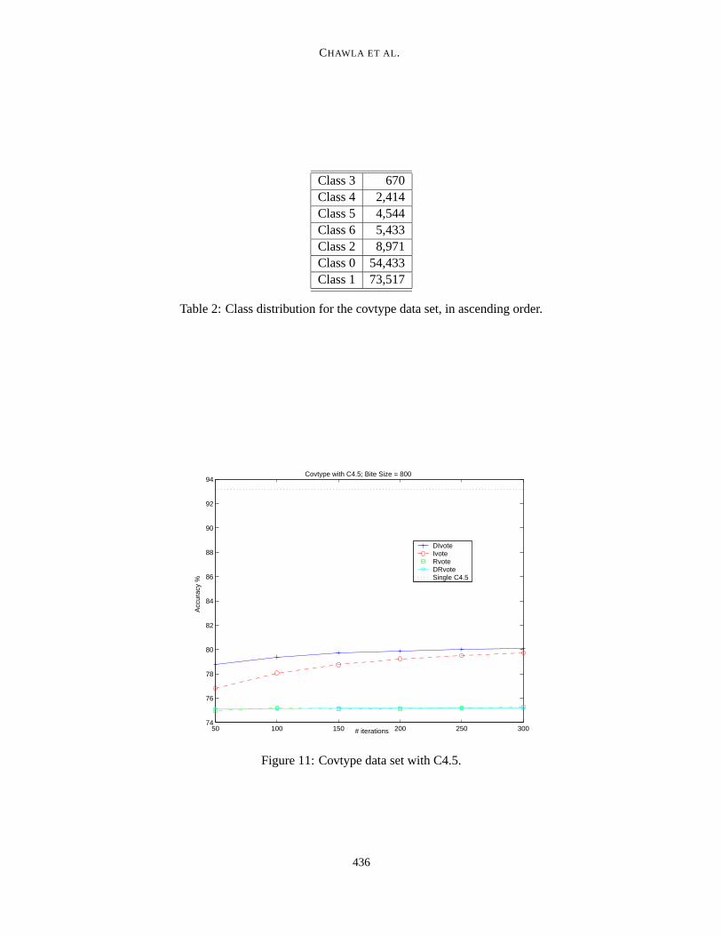
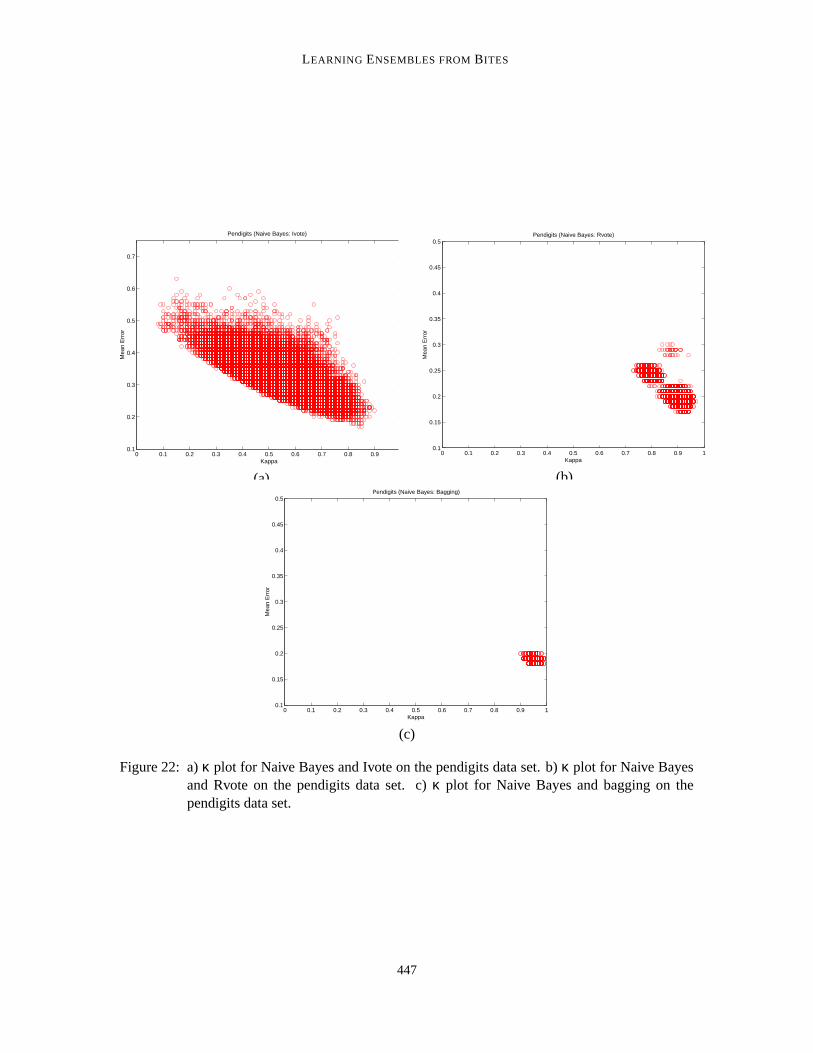
Table 5 shows the classification accuracies obtained from learning Naive Bayes classifiers onthe letter and pendigits data sets. Figures 21 to 22 highlight the κ results on both the pendigits andletter data sets. As is evident from the figures, Ivoted classifiers are more diverse (and accurate) thanboth Rvoted and bagged classifiers. This result is not very surprising, as Ivote/DIvote classifiers arelearned on bites derived from importance sampling, and each of these bites can look very differentdue to the heavier sampling from more difficult examples. Although a spread of κ values is observedfor Rvote with the pendigits data set, this spread is prevalent at 0.7 ≤ κ ≤ 1.0. Higher κ valuesindicate a higher degree of agreement between the different pairs of classifiers.

10. Conclusion

We proposed a distributed framework for pasting Ivotes by dividing a training set into n disjointpartitions and building hundreds of classifiers (using very small training sets) on each disjoint par-tition. The main conclusion of our work is that pasting DIvotes is a promising approach for very

4. The source code was downloaded from http://fuzzy.cs.uni-magdeburg.de/∼borgelt/software.html.

444


0 0.1 0.2 0.3 0.4 0.5 0.6 0.7 0.8 0.9 10.35

0.4

0.45

0.5

0.55

0.6

0.65

0.7

0.75Letter: DIvote

Kappa

Mea

n E

rror

(a)

0 0.1 0.2 0.3 0.4 0.5 0.6 0.7 0.8 0.9 10.35

0.4

0.45

0.5

0.55

0.6

0.65

0.7

0.75Letter: DRvote

Kappa

Mea

n E

rror

(b)

Figure 19: a) κ Plot for DIvote with C4.5 on the letter data set. b) κ Plot for DRvote with C4.5 onthe letter data set.

(a) (b)

Figure 20: a) κ plot for DIvote and Jones data set. b) κ plot for DRvote and Jones data set.

445

CHAWLA ET AL.

0 0.1 0.2 0.3 0.4 0.5 0.6 0.7 0.8 0.9 10.3

0.35

0.4

0.45

0.5

0.55

Letter (Naive Bayes and Ivote)

Kappa

Mea

n E

rror

(a)

0 0.1 0.2 0.3 0.4 0.5 0.6 0.7 0.8 0.9 10.3

0.32

0.34

0.36

0.38

0.4

0.42

0.44

0.46

0.48

0.5Letter (Naive Bayes: Rvote)

Kappa

Mea

n E

rror

(b)

0 0.1 0.2 0.3 0.4 0.5 0.6 0.7 0.8 0.9 10.2

0.25

0.3

0.35

0.4

0.45

0.5Letter dataset: Bagging and Naive Bayes

Kappa

Mea

n E

rror

(c)

Figure 21: a) κ plot for Naive Bayes and Ivote on the letter data set. b) κ plot for Naive Bayes andRvote on the letter data set. c) κ plot for Naive Bayes and bagging on the letter data set.

446


0 0.1 0.2 0.3 0.4 0.5 0.6 0.7 0.8 0.9 10.1

0.2

0.3

0.4

0.5

0.6

0.7

Pendigits (Naive Bayes: Ivote)

Kappa

Mea

n E

rror

(a)

0 0.1 0.2 0.3 0.4 0.5 0.6 0.7 0.8 0.9 10.1

0.15

0.2

0.25

0.3

0.35

0.4

0.45

0.5Pendigits (Naive Bayes: Rvote)

Kappa

Mea

n E

rror

(b)

0 0.1 0.2 0.3 0.4 0.5 0.6 0.7 0.8 0.9 10.1

0.15

0.2

0.25

0.3

0.35

0.4

0.45

0.5Pendigits (Naive Bayes: Bagging)

Kappa

Mea

n E

rror

(c)

Figure 22: a) κ plot for Naive Bayes and Ivote on the pendigits data set. b) κ plot for Naive Bayesand Rvote on the pendigits data set. c) κ plot for Naive Bayes and bagging on thependigits data set.

447

CHAWLA ET AL.

large data sets. Data sets too large to be handled practically in the memory of a typical computerare appropriately handled by simple partitioning into disjoint subsets, and adding another level oflearning by pasting DIvotes or DRvotes on each of the disjoint subsets. We show that for almostall the data sets, using decision trees and neural networks, DIvote achieves classification accuracycomparable to Ivote (sometimes better), and almost always better than learning a single classifier.We evaluated DIvote and Ivote on data sets coming from various domains, and for almost all thecases they achieve significantly better classification accuracies than a single classifier.

DIvote is scalable as it never requires the learning set size to be greater than a very small pro-portion of the entire training set. Each processor works independently, without requiring commu-nication at any stage of learning. The end result is an ensemble of hundreds of DIvote classifiers.We also conclude that pasting DIvotes is more accurate than pasting DRvotes. We believe that thecombined effects of diversity, good coverage, and importance sampling are helping DIvote and Iv-ote. It is significant that DIvote does much better than the simplistic version of pasting small votesin a distributed scenario. Moreover, we observe that with DIvote and Ivote, the accuracy growsfast initially during learning, and then slowly plateaus. Particularly, with neural networks feweriterations of DIvoting are needed to vastly improve over learning a single classifier from the entiretraining set. Neural networks, particularly, can get slowed down significantly in the training phasewhen learning from very large data sets. DIvote is a promising approach to reduce the learning timewith neural networks even on very large data sets.

Using κ (diversity) plots, we support the theory that given an ensemble of diverse classifiers, animprovement in the accuracy can be observed. We note that DIvote provides the most significantimprovement of almost 18% (relative improvement of 34%) in the difficult, non-homogeneous Pro-tein Prediction problem over learning a single classifier using C4.5. Thus, the ensemble of diverseDIvote classifiers counters the effect of overfitting and improves the generalization.

Another important contribution of our work is comparison to the distributed boosting approach.We conclude that DIvote achieves classification accuracies similar to the distributed boosting ap-proach, with no inter-processor communication at any stage of learning.

The DIvote framework is naturally applicable to the scenario in which data sets for a problemare already distributed. At each of the distributed sites multiple classifiers can be built, and the onlycommunication required is the learned classifiers at the end of training. Inter-processor communica-tion can become a bottleneck if an exchange of data is required across various nodes or processors.Moreover, one can easily conceptualize the applicability of DIvote on a cluster of workstations in alab, where each workstation independently works on a part of the problem in its main memory.

Acknowledgments

This work was supported in part by the United States Department of Energy through the San-dia National Laboratories ASCI VIEWS Data Discovery Program, contract number DE-AC04-76DO00789. This work was also supported in part by National Science Foundation under grantEIA-0130768. We would like to thank the reviewers for their useful comments. We would liketo thank Robert Banfield for his help with the experiment on ASCI Blue Supercomputer. We alsothank Aleksander Lazarevic for providing us the training and testing sets of the data sets used in thedistributed boosting paper.

448


References

Seventh ACM SIGKDD International Conference on Knowledge Discovery and Data Mining, SanFrancisco, CA, 2001. ACM.

R. E. Banfield, L. O. Hall, K. W. Bowyer, and W. P. Kegelmeyer. A new ensemble diversity measureapplied to thinning ensembles. In Multiple Classifier Systems Workshop, pages 306–316, Surrey,UK, 2003.

E. Bauer and R. Kohavi. An empirical comparison of voting classification algorithms: Bagging,boosting and variants. Machine Learning, 36(1,2), 1999.

H. M. Berman, J. Westbrook, Z. Feng, G. Gilliland, T. N. Bhat, H. Weissig, I. N. Shindyalov,and P. E. Bourne. The protein data bank. Nucleic Acids Research, 28:235–242, 2000.http://www.pdb.org/.

C. L. Blake and C. J. Merz. UCI repository of machine learning databases.http://www.ics.uci.edu/∼mlearn/MLRepository.html, 1998.

L. Breiman. Bagging predictors. Machine Learning, 24(2):123–140, 1996.

L. Breiman. Pasting bites together for prediction in large data sets. Machine Learning, 36(2):85–103, 1999.

L. Breiman. Random forests. Machine Learning, 45(1):5–32, 2001.

P. Chan and S. Stolfo. Towards parallel and distributed learning by meta-learning. In Working NotesAAAI Workshop on Knowledge Discovery and Databases, pages 227–240, San Mateo, CA, 1993.

N. V. Chawla, S. Eschrich, and L. O. Hall. Creating ensembles of classifiers. In First IEEE Inter-national Conference on Data Mining, pages 581 – 583, San Jose, CA, 2000.

N. V. Chawla, L. O. Hall, K. W. Bowyer, T. E. Moore, and W. P. Kegelmeyer. Distributed pastingof small votes. In Third International Workshop on Multiple Classifier Systems, pages 52 – 61,Cagliari, Italy, 2002a.

N. V. Chawla, T. E. Moore, L. O. Hall, K. W. Bowyer, C. Springer, and W. P. Kegelmeyer. Dis-tributed learning with bagging-like performance. Pattern Recognition Letters, 24(1-3):455 – 471,2002b.

N. V. Chawla, T. E. Moore, Jr., L. O. Hall, K. W. Bowyer, W. P. Kegelmeyer, and C. Springer. Inves-tigation of bagging-like effects and decision trees versus neural nets in protein secondary structureprediction. In ACM SIGKDD Workshop on Data Mining in Bio-Informatics, San Francisco, CA,2001.

D. J. Spiegelhalter D. Michie and C. C. Taylor. Machine Learning, Neural and Statistical Classifi-cation. Ellis Horwood, 1994.

T. Dietterich. An empirical comparison of three methods for constructing ensembles of decisiontrees: bagging, boosting and randomization. Machine Learning, 40(2):139 – 157, 2000.

449

CHAWLA ET AL.

P. Domingos. Using partitioning to speed up specific-to-general rule induction. In AAAI Workshopon Integrating Multiple Learned Models, pages 29–34, Portland, OR, 1996.

R. Duda, P. Hart, and D. Stork. Pattern Classification. Wiley-Interscience, 2001.

S. Eschrich, N. V. Chawla, and L. O. Hall. Learning to predict in complex biological domains.Journal of System Simulation, 2:1464 – 1471, 2002.

S. E. Fahlman and C. Lebiere. The cascade-correlation learning architecture. In Advances in NeuralInformation Processing Systems 2, Vancouver, Canada, 1990. Morgan Kaufmann.

U. M. Fayyad, G. Piatetsky-Shapiro, and P. Smyth. Advances in Knowledge Discovery and DataMining, chapter From data mining to knowledge discovery: An overview. AAAI Press, MenloPark, CA, 1996.

Y. Freund and R. Schapire. Experiments with a new boosting algorithm. In Thirteenth InternationalConference on Machine Learning, Bari, Italy, 1996.

G. Giacinto and F. Roli. An approach to automatic design of multiple classifier systems. PatternRecognition Letters, 22:25 – 33, 2001.

I. J. Good. The Estimation of Probabilities: An essay on modern Bayesian methods. MIT Press,1965.

L. O. Hall, K. W. Bowyer, N. V. Chawla, T. E. Moore, and W. P. Kegelmeyer. Avatar: Adaptive Vi-sualization Aid for Touring and Recovery. Technical Report SAND2000-8203, Sandia NationalLabs, 2000.

L. O. Hall, N. V. Chawla, K. W. Bowyer, and W.P Kegelmeyer. Learning rules from distributeddata. In Workshop of Fifth ACM SIGKDD International Conference on Knowledge Discoveryand Data Mining, San Diego, CA, 1999.

T. Ho. Random subspace method for constructing decision forests. IEEE Transactions on PAMI,20(8):832 – 844, 1998.

D. T. Jones. Protein secondary structure prediction based on decision-specific scoring matrices.Journal of Molecular Biology, 292:195–202, 1999.

L. Kuncheva and C. Whitaker. Measures of diversity in classifier ensembles and their relationshipwith the ensemble accuracy. Machine Learning, 51:181 – 207, 2003.

L. Kuncheva, C. Whitaker, C. Shipp, and R. Duin. Is independence good for combining classi-fiers? In Proceedings of 15th International Conference on Pattern Recognition, pages 168 – 171,Barcelona, Spain, September 2000.

P. Latinne, O. Debeir, and C. Decaestecker. Limiting the number of trees in random forests. InJ. Kittler and F. Roli, editors, Multiple Classifier Systems, Second International Workshop, pages178 – 187, Cambridge, UK, 2001. Springer.

450


A. Lazarevic and Z. Obradovic. Boosting algorithms for parallel and distributed learning. Dis-tributed and Parallel Databases Journal, Special Issue on Parallel and Distributed Data Mining,11:203 – 229, 2002.

N. Leavitt. Data mining for the corporate masses. In IEEE Computer. IEEE Computer Society, May2002.

Lawrence Livermore National Laboratories. ASCI Blue Pacific.http://www.llnl.gov/asci/platforms/bluepac.

Lawrence Livermore National Laboratories. Protein Structure Prediction Center.http://predictioncenter.llnl.gov/, 1999.

R. Musick, J. Catlett, and S. Russell. Decision theoretic subsampling for induction on largedatabases. In Proceedings of Tenth International Conference on Machine Learning, pages 212 –219, Amherst, MA, 1993.

C. Perlich, F. Provost, and J. Simonoff. Tree induction vs. logistic regression: A learning-curveanalysis. Journal of Machine Learning Research, 4:211–255, 2003.

F. Provost and D. N. Hennessy. Scaling up: Distributed machine learning with cooperation. InProceedings of the Thirteenth National Conference on Artificial Intelligence, AAAI ’96, pages74–79, Portland, Oregon, 1996.

F. Provost and V. Kolluri. A survey of methods for scaling up inductive algorithms. Data Miningand Knowledge Discovery, 3(2):131–169, 1999.

F. J. Provost, D. Jensen, and T. Oates. Efficient progressive sampling. In Proceedings of the FifthACM SIGKDD International Conference on Knowledge Discovery and Data Mining, pages 23–32, San Diego, CA, 1999.

J. R. Quinlan. C4.5: Programs for Machine Learning. Morgan Kaufmann, San Mateo, CA, 1992.

D. B. Skalak. The sources of increased accuracy for two proposed boosting algorithms. In AAAIIntegrating Multiple Learned Models Workshop, Portland, Oregon, 1996.

W. N. Street and Y. Kim. A streaming ensemble algorithm (SEA) for large-scale classification.In Proceedings of seventh International Conference on Knowledge Discovery and Data Mining,pages 377–382, 2001. San Francisco, CA.

451

Date post:	23-Mar-2019
Category:	Documents
Upload:	buinhu
View:	220 times
Download:	0 times

Learning Ensembles from Bites: A Scalable and Accurate...

Documents