Learning from Limited Demonstrations

Beomjoon Kim

School of Computer ScienceMcGill University

Montreal, Quebec, Canada

Amir-massoud Farahmand

School of Computer ScienceMcGill University

Montreal, Quebec, Canada

Joelle Pineau

School of Computer ScienceMcGill University

Montreal, Quebec, Canada

Doina Precup

School of Computer ScienceMcGill University

Montreal, Quebec, Canada

Abstract

We propose a Learning from Demonstration (LfD) algorithm which leverages ex-pert data, even if they are very few or inaccurate. We achieve this by using bothexpert data, as well as reinforcement signals gathered through trial-and-error inter-actions with the environment. The key idea of our approach, Approximate PolicyIteration with Demonstration (APID), is that expert’s suggestions are used to de-fine linear constraints which guide the optimization performed by ApproximatePolicy Iteration. We prove an upper bound on the Bellman error of the estimatecomputed by APID at each iteration. Moreover, we show empirically that APIDoutperforms pure Approximate Policy Iteration, a state-of-the-art LfD algorithm,and supervised learning in a variety of scenarios, including when very few and/orsuboptimal demonstrations are available. Our experiments include simulations aswell as a real robot path-finding task.

1 Introduction

Learning from Demonstration (LfD) is a practical framework for learning complex behaviour poli-cies from demonstration trajectories produced by an expert. In most conventional approaches toLfD, the agent observes mappings between states and actions in the expert trajectories, and uses su-pervised learning to estimate a function that can approximately reproduce this mapping. Ideally, thefunction (i.e., policy) should also generalize well to regions of the state space that are not observedin the demonstration data. Many of the recent methods focus on incrementally querying the expert inappropriate regions of the state space to improve the learned policy, or to reduce uncertainty [1, 2, 3].Key assumptions of most these works are that (1) the expert exhibits optimal behaviour, (2) the ex-pert demonstrations are abundant, and (3) the expert stays with the learning agent throughout thetraining. In practice, these assumptions significantly reduce the applicability of LfD.

We present a framework that leverages insights and techniques from the reinforcement learning(RL) literature to overcome these limitations of the conventional LfD methods. RL is a generalframework for learning optimal policies from trial-and-error interactions with the environment [4,5]. The conventional RL approaches alone, however, might have difficulties in achieving a goodperformance from relatively little data. Moreover, they are not particularly cautious to risk involvedin trial-and-error learning, which could lead to catastrophic failures. A combination of both expertand interaction data (i.e., mixing LfD and RL), however, offers a tantalizing way to effectivelyaddress challenging real-world policy learning problems under realistic assumptions.

Our primary contribution is a new algorithmic framework that integrates LfD, tackled using a largemargin classifier, with a regularized Approximate Policy Iteration (API) method. The method is

1

formulated as a coupled constraint convex optimization, in which expert demonstrations define aset of linear constraints in API. The optimization is formulated in a way that permits mistakes inthe demonstrations provided by the expert, and also accommodates variable availability of demon-strations (i.e., just an initial batch or continued demonstrations). We provide a theoretical analysisdescribing an upper bound on the Bellman error achievable by our approach.

We evaluate our algorithm in a simulated environment under various scenarios, such as varying thequality and quantity of expert demonstrations. In all cases, we compare our algorithm with Least-Square Policy Iteration (LSPI) [6], a popular API method, as well as with a state-of-the-art LfDmethod, Dataset Aggregation (DAgger) [1]. We also evaluate the algorithm’s practicality in a realrobot path finding task, where there are few demonstrations, and exploration data is expensive dueto limited time. In all of the experiments, our method outperformed LSPI, using fewer explorationdata and exhibiting significantly less variance. Our method also significantly outperformed DatasetAggregation (DAgger), a state-of-art LfD algorithm, in cases where the expert demonstrations arefew or suboptimal.

2 Proposed Algorithm

We consider a continuous-state, finite-action discounted MDP (X ,A, P,R, γ), where X is ameasurable state space, A is a finite set of actions, P : X × A → M(X ) is the transitionmodel, R : X × A → M(R) is the reward model, and γ ∈ [0, 1) is a discount factor.1 Letr(x, a) = E [R(·|x, a)], and assume that r is uniformly bounded by Rmax. A measurable mappingπ : X → A is called a policy. As usual, V π and Qπ denote the value and action-value function forπ, and V ∗ and Q∗ denote the corresponding value functions for the optimal policy π∗ [5].

Our algorithm is couched in the framework of API [7]. A standard API algorithm starts with aninitial policy π0. At the (k+1)th iteration, given a policy πk, the algorithm approximately evaluatesπk to find Qk, usually as an approximate fixed point of the Bellman operator Tπk : Qk ≈ TπkQk.2This is called the approximate policy evaluation step. Then, a new policy πk+1 is computed, whichis greedy with respect to Qk. There are several variants of API that mostly differ on how the approx-imate policy evaluation is performed. Most methods attempt to exploit the structures in the valuefunction [8, 9, 10, 11], but in some problems one might have extra information about the structureof good or optimal policies as well. This is precisely our case, since we have expert demonstrations.

To develop the algorithm, we start with regularized Bellman error minimization, which is a commonflavour of policy evaluation used in API. Suppose that we want to evaluate a policy π given a batchof data DRL = (Xi, Ai)ni=1 containing n examples, and that the exact Bellman operator Tπ isknown. Then, the new value function Q is computed as:

Q ← argminQ∈F |A|

Q− TπQ2n + λJ

2(Q), (1)

where F |A| is the set of action-value functions, the first term is the squared Bellman error evaluatedon the data,3 J2(Q) is the regularization penalty, which can prevent overfitting when F |A| is com-plex, and λ > 0 is the regularization coefficient. The regularizer J(Q) measures the complexity offunction Q. Different choices of F |A| and J lead to different notions of complexity, e.g., variousdefinitions of smoothness, sparsity in a dictionary, etc. For example, F |A| could be a reproducingkernel Hilbert space (RKHS) and J its corresponding norm, i.e., J(Q) = Q

H.

In addition to DRL, we have a set of expert examples DE = (Xi,πE(Xi))mi=1, which we wouldlike to take into account in the optimization process. The intuition behind our algorithm is thatwe want to use the expert examples to “shape” the value function where they are available, whileusing the RL data to improve the policy everywhere else. Hence, even if we have few demonstrationexamples, we can still obtain good generalization everywhere due to the RL data.

To incorporate the expert examples in the algorithm one might require that at the states Xi from DE,the demonstrated action πE(Xi) be optimal, which can be expressed as a large-margin constraint:

1For a space Ω with σ-algebra σΩ, M(Ω) denotes the set of all probability measures over σΩ.2For discrete state spaces, (TπkQ)(x, a) = r(x, a) + γ

x P (x|x, a)Q(x,πk(x

)).3Q− TπQ2n 1

n

ni=1 |Q(Xi, Ai)− (TπQ)(Xi, Ai)|2 with (Xi, Ai) from DRL.

2

Q(Xi,πE(Xi)) − maxa∈A\πE(Xi) Q(Xi, a) ≥ 1. However, this might not always be feasible, ordesirable (if the expert itself is not optimal), so we add slack variables ξi ≥ 0 to allow occasionalviolations of the constraints (similar to soft vs. hard margin in the large-margin literature [12]). Thepolicy evaluation step can then be written as the following constrained optimization problem:

Q ← argminQ∈F |A|,ξ∈Rm

+

Q− TπQ2n + λJ

2(Q) +α

m

m

i=1

ξi (2)

s.t. Q(Xi,πE(Xi))− maxa∈A\πE(Xi)

Q(Xi, a) ≥ 1− ξi. for all (Xi,πE(Xi)) ∈ DE

The parameter α balances the influence of the data obtained by the RL algorithm (generally by trial-and-error) vs. the expert data. When α = 0, we obtain (1), while when α → ∞, we essentiallysolve a structured classification problem based on the expert’s data [13]. Note that the right side ofthe constraints could also be multiplied by a coefficient ∆i > 0, to set the size of the acceptablemargin between the Q(Xi,πE(Xi)) and maxa∈A\πE(Xi) Q(Xi, a). Such a coefficient can then beset adaptively for different examples. However, this is beyond the scope of the paper.

The above constrained optimization problem is equivalent to the following unconstrained one:

Q ← argminQ∈F|A|

Q− TπQ2n + λJ2(Q) +αm

m

i=1

1−

Q(Xi,πE(Xi))− max

a∈A\πE(Xi)Q(Xi, a)

+

(3)

where [1− z]+ = max0, 1− z is the hinge loss.

In many problems, we do not have access to the exact Bellman operator Tπ , but only to sam-ples DRL = (Xi, Ai, Ri, X

i)ni=1 with Ri ∼ R(·|Xi, Ai) and X

i ∼ P (·|Xi, Ai). In thiscase, one might want to use the empirical Bellman error Q − TπQ2n (with (TπQ)(Xi, Ai) Ri + γQ(X

i,π(Xi)) for 1 ≤ i ≤ n) instead of Q − TπQ2n. It is known, however, that this is a

biased estimate of the Bellman error, and does not lead to proper solutions [14]. One approach toaddress this issue is to use the modified Bellman error [14]. Another approach is to use ProjectedBellman error, which leads to an LSTD-like algorithm [8]. Using the latter idea, we formulate ouroptimization as:

Q ← argminQ∈F |A|,ξ∈Rm

+

Q− hQ

2

n+ λJ

2(Q) +α

m

m

i=1

ξi (4)

s.t. hQ = argminh∈F |A|

h− TπQ

2

n+ λhJ

2(h)

Q(Xi,πE(Xi))− maxa∈A\πE(Xi)

Q(Xi, a) ≥ 1− ξi. for all (Xi,πE(Xi)) ∈ DE

Here λh > 0 is the regularization coefficient for hQ, which might be different from λ. For somechoices of the function space F |A| and the regularizer J , the estimate hQ can be found in closed-form. For example, one can use linear function approximators h(·) = φ(·)u and Q(·) = φ(·)wwhere u,w ∈ Rp are parameter vectors and φ(·) ∈ Rp is a vector of p linearly independent basisfunctions defined over the space of state-action pairs. Using L2-regularization, J2(h) = uu andJ2(Q) = ww, the best parameter vector u∗ can be obtained as a function of w by solving a ridgeregression problem:

u∗(w) =ΦΦ+ nλhI

−1Φ(r + γΦw),

where Φ, Φ and r are the feature matrices and reward vector, respectively: Φ =(φ(Z1), . . . ,φ(Zn))

, Φ = (φ(Z 1), . . . ,φ(Z

n))

, r = (R1, . . . , Rn), with Zi = (Xi, Ai)

and Z i = (X

i,π(Xi)) (for data belonging to DRL). More generally, as discussed above, we might

choose the function space F |A| to be a reproducing kernel Hilbert space (RKHS) and J to be itscorresponding norm, which provides the flexibility of working with a nonparametric representationwhile still having a closed-form solution for hQ. We do not provide the detail of formulation heredue to space constraints.

The approach presented so far tackles the policy evaluation step of the API algorithm. As usualin API, we alternate this step with the policy improvement step (i.e., greedification). The resultingalgorithm is called Approximate Policy Iteration with Demonstration (APID).

3

Up to this point, we have left open the problem of how the datasets DRL and DE are obtained. Thesedatasets might be regenerated at each iteration, or they might be reused, depending on the availabilityof the expert and the environment. In practice, if the expert data is rare, DE will be a single fixedbatch, but DRL could be increased, e.g., by running the most current policy (possibly with someexploration) to collect more data. The approach used should be tailored to the application. Notethat the values of the regularization coefficients as well as α should ideally change from iteration toiteration as a function of the number of samples as well as the value function Qπk . The choice ofthese parameters might be automated by model selection [15].

3 Theoretical Analysis

In this section we focus on the kth iteration of APID and consider the solution Q to the optimizationproblem (2). The theoretical contribution is an upper bound on the true Bellman error of Q. Such anupper bound allows us to use error propagation results [16, 17] to provide a performance guaranteeon the value of the outcome policy πK (the policy obtained after K iterations of the algorithm)compared to the optimal value function V ∗. We make the following assumptions in our analysis.

Assumption A1 (Sampling) DRL contains n independent and identically distributed (i.i.d.) samples(Xi, Ai)

i.i.d.∼ νRL ∈ M(X × A) where νRL is a fixed distribution (possibly dependent on k) andthe states in DE = (Xi,πE(Xi)mi=1 are also drawn i.i.d. Xi

i.i.d.∼ νE ∈ M(X ) from an expertdistribution νE. DRL and DE are independent from each other. We denote N = n+m.

Assumption A2 (RKHS) The function space F |A| is an RKHS defined by a kernel function K :

(X × A) × (X × A) → R, i.e., F |A| =z →

Ni=1 wiK(z, Zi) : w ∈ RN

with ZiNi=1 =

DRL ∪ DE. We assume that supz∈X×A K (z, z) ≤ 1. Moreover, the function space F |A| is Qmax-bounded.

Assumption A3 (Function Approximation Property) For any policy π, Qπ ∈ F |A|.

Assumption A4 (Expansion of Smoothness) For all Q ∈ F |A|, there exist constants 0 ≤ LR, LP <

∞, depending only on the MDP and F |A|, such that for any policy π, J(TπQ) ≤ LR + γLPJ(Q).

Assumption A5 (Regularizers) The regularizer functionals J : B(X ) → R and J : B(X ×A) →R are pseudo-norms on F and F |A|, respectively,4 and for all Q ∈ F |A| and a ∈ A, we haveJ(Q(·, a)) ≤ J(Q).

Some of these assumptions are quite mild, while some are only here to simplify the analysis, butare not necessary for practical application of the algorithm. For example, the i.i.d. assumption A1can be relaxed using independent block technique [18] or other techniques to handle dependent data,e.g., [19]. The method is certainly not specific to RKHS (Assumption A2), so other function spacescan be used without much change in the proof. Assumption A3 holds for “rich” enough functionspaces, e.g., universal kernels satisfy it for reasonable Qπ . Assumption A4 ensures that if Q ∈ F |A|

then TπQ ∈ F |A|. It holds if F |A| is rich enough and the MDP is “well-behaving”. Assumption A5is mild and ensures that if we control the complexity of Q ∈ F |A|, the complexity of Q(·, a) ∈ Fis controlled too. Finally, note that focusing on the case when we have access to the true Bellmanoperator simplifies the analysis while allowing us to gain more understanding about APID. We arenow ready to state the main theorem of this paper.

Theorem 1. For any fixed policy π, let Q be the solution to the optimization problem (2) with thechoice of α > 0 and λ > 0. If Assumptions A1–A5 hold, for any n,m ∈ N and 0 < δ < 1, withprobability at least 1− δ we have

4 B(X ) and B(X ×A) denote the space of bounded measurable functions defined on X and X ×A. Herewe are slightly abusing notation as the same symbol is used for the regularizer over both spaces. However, thisshould not cause any confusion since the identity of the regularizer should always be clear from the context.

4

Q− TπQ2

νRL≤ 64Qmax

√n+mn

(1 + γLP )

√R2

max + α√λ

+ LR

+

min

2αEX∼νE

1−

Qπ(X,πE(X))− max

a∈A\πE(X)Qπ(X, a))

+

+ λJ2(Qπ),

2 QπE − TπQπE2νRL+ 2αEX∼νE

1−

QπE (X,πE(X))− max

a∈A\πE(X)QπE (X, a))

+

+

λJ2(QπE )

+ 4Q2

max

2 ln(4/δ)

n+

6 ln(4/δ)n

+ α

20(1 + 2Qmax) ln(8/δ)3m

.

The proof of this theorem is in the supplemental material. Let us now discuss some aspects ofthe result. The theorem guarantees that when the amount of RL data is large enough (n m),we indeed minimize the Bellman error if we let α → 0. In that case, the upper bound wouldbe OP (

1√nλ

) + minλJ2(Qπ), 2 QπE − TπQπE2νRL+ λJ2(QπE ). Considering only the first

term inside min, the upper bound is minimized by the choice of λ = [n1/3J4/3(Qπ)]−1, whichleads to OP (J2/3(Qπ)n−1/3) behaviour of the upper bound. The bound shows that the difficulty oflearning depends on J(Qπ), which is the complexity of the true (but unknown) action-value functionQπ measured according to J in F |A|. Note that Qπ might be “simple” with respect to some choiceof function space/regularizer, but complex in another one. The choice of F |A| and J reflects priorknowledge regarding the function space and complexity measure that are suitable.

When the number of samples n increases, we can afford to increase the size of the function spaceby making λ smaller. Since we have two terms inside min, the complexity of the problem mightactually depend on 2 QπE − TπQπE2νRL

+λJ2(QπE ), which is the Bellman error of QπE (the trueaction-value function of the expert) according to π plus the complexity of QπE in F |A|. Roughlyspeaking, if π is close to πE , the Bellman error would be small. Two remarks are in order. First, thisresult does not provide a proper upper bound on the Bellman error when m dominates n. This isto be expected, because if π is quite different from πE and we do not have enough samples in DRL,we cannot guarantee that the Bellman error, which is measured according to π, will be small. But,one can still provide a guarantee by choosing a large α and using a margin-based error bound (cf.Section 4.1 of [20]). Second, this upper bound is not optimal, as we use a simple proof techniquebased on controlling the supremum of the empirical process. More advanced empirical processestechniques can be used to obtain a faster error rate (cf. [12]).

4 Experiments

We evaluate APID on a simulated domain, as well as a real robot path-finding task. In the simulatedenvironment, we compare APID against other benchmarks under varying availability and optimalityof the expert demonstrations. In the real robot task, we evaluate the practicality of deploying APIDon a live system, especially when DRL and DE are both expensive to obtain.

4.1 Car Brake Control Simulation

In the vehicle brake control simulation [21], the agent’s goal is reach a target velocity, then maintainthat target. It can either press the acceleration pedal or the brake pedal, but not both simultaneously.A state is represented by four continuous-valued features: target and current velocities, currentpositions of brake pedal and acceleration pedal. Given a state, the learned policy has to output oneof five actions: acceleration up, acceleration down, brake up, brake down, do nothing. The rewardis −10 times the error in velocity. The initial velocity is set to 2m/s, and the target velocity is setto 7m/s. The expert was implemented using the dynamics between the pedal pressure and outputvelocity, from which we calculate the optimal velocity at each state. We added random noise to thedynamics to simulate a realistic scenario, in which the output velocity is governed by factors suchas friction and wind. The agent has no knowledge of the dynamics, and receives only DE and DRL.

For all experiments, we used a linear Radial Basis Function (RBF) approximator for the value func-tion and CVX, a package for specifying and solving convex programs [22], to solve the optimization

5

1 2 3 4 5 6 7 8 9 10−80

−70

−60

−50

−40

−30

−20

−10

0

10

20

Number of Iterations

Av

era

ge

Re

wa

rds

APID

LSPI

Supervised

(a)

1 2 3 4 5 6 7 8 9 10−80

−70

−60

−50

−40

−30

−20

−10

0

10

20

Number of Iterations

Av

era

ge

Re

wa

rds

APID

LSPI

Supervised

(b)

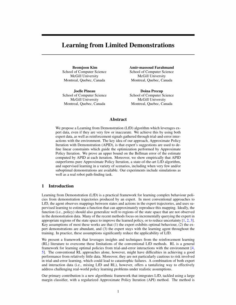
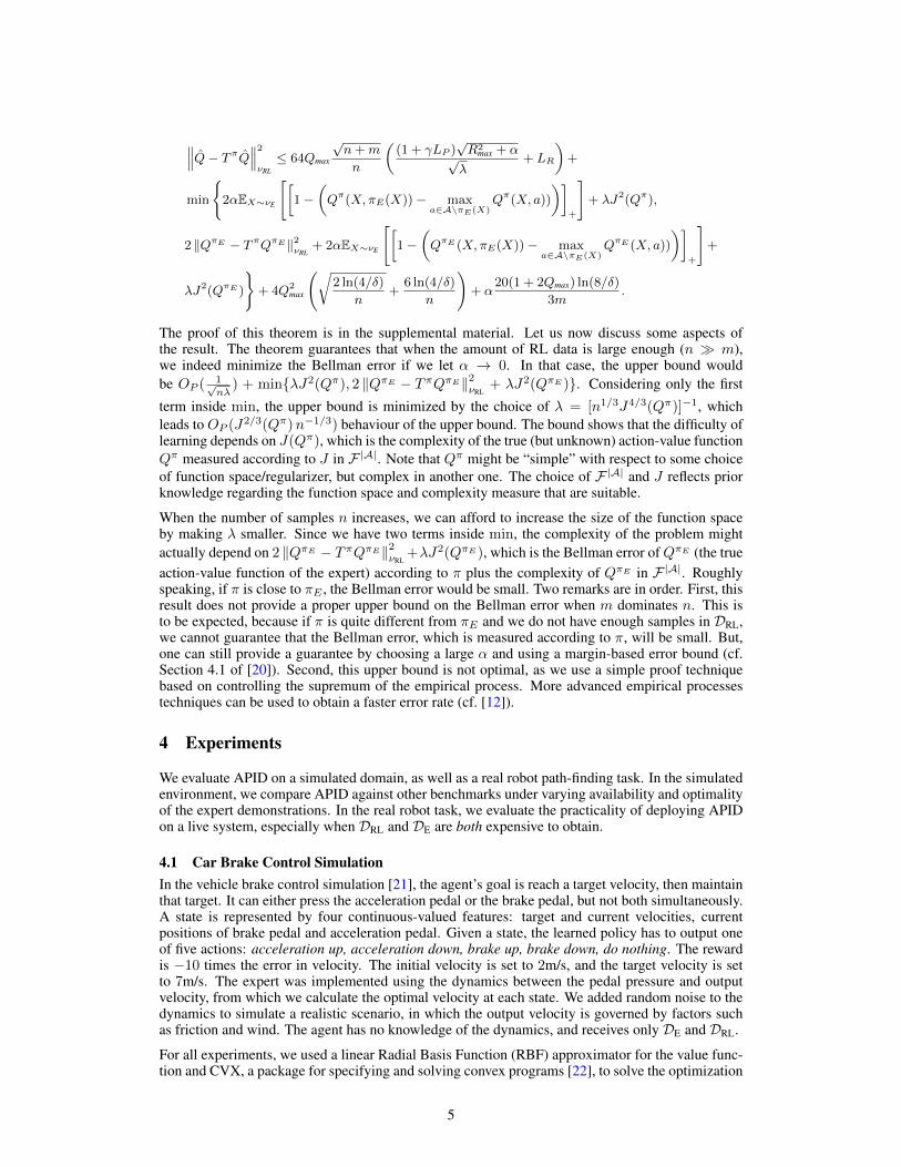
Figure 1: (a) Average reward with m = 15 optimal demonstrations. (b) Average reward withm = 100 sub-optimal demonstrations. Each iteration adds 500 new RL data to APID and LSPI,while the expert data stays the same. First iteration has n = 500 −m for APID. LSPI treats all thedata at this iteration RL data.

problem (4). We set αm to 1 if the expert is optimal and 0.01 otherwise. The regularization param-

eter was set according to 1/√n+m. We averaged results over 10 runs and computed confidence

intervals as well. We compare APID with the regularized version of LSPI [6] in all the experiments.Depending on the availability of expert data, we either compare APID with the standard supervisedLfD, or DAgger [1], a state-of-the-art LfD algorithm that has strong theoretical guarantees and goodempirical performance when the expert is optimal. DAgger is designed to query for more demon-strations at each iteration; then, it aggregates all demonstrations and trains a new policy. The numberof queries in DAgger increases linearly with the task horizon. For Dagger and supervised LfD, weuse random forests to train the policy.

We first consider the case with little but optimal expert data, with task horizon 1000. At eachiteration, the agent gathers more RL data using a random policy. In this case, shown in Figure 1a,LSPI performs worse than APID on average, and it also has much higher variance, especially whenDRL is small. This is consistent with empirical results in [6], in which LSPI showed significantvariance even for simple tasks. In the first iteration, APID has moderate variance, but it is quicklyreduced in the next iteration. This is due to the fact that expert constraints impose a particular shapeto the value function, as noted in Section 2. The supervised LfD performs the worst, as the amount ofexpert data is insufficient. Results for the case in which the agent has more but sub-optimal expertdata are shown in Figure 1b. Here, with probability 0.5 the expert gives a random action ratherthan the optimal action. Compared to supervised LfD, APID and LSPI are both able to overcomesub-optimality in the expert’s behaviour to achieve good performance, by leveraging the RL data.

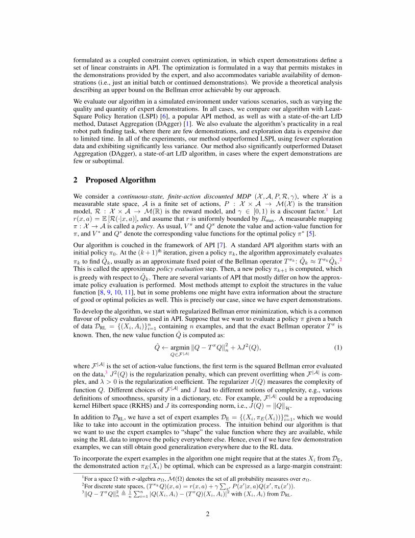
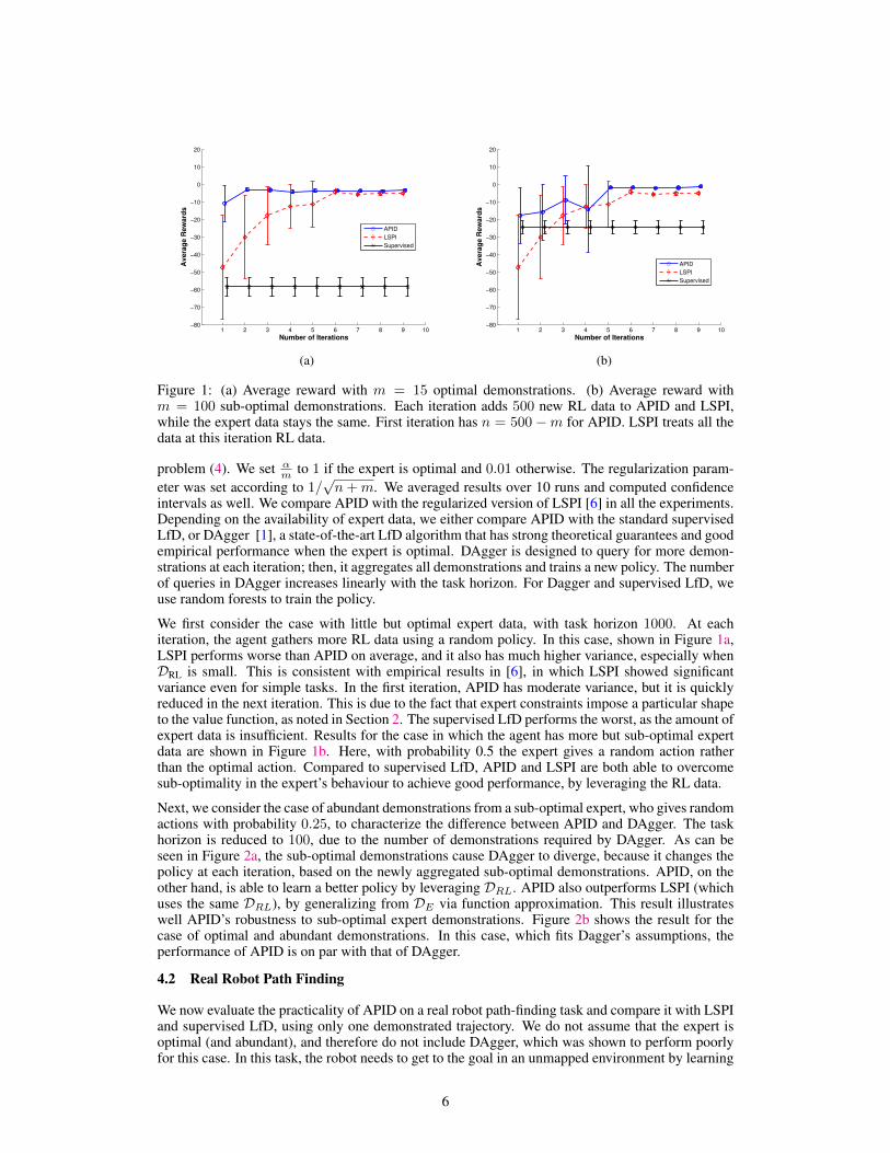
Next, we consider the case of abundant demonstrations from a sub-optimal expert, who gives randomactions with probability 0.25, to characterize the difference between APID and DAgger. The taskhorizon is reduced to 100, due to the number of demonstrations required by DAgger. As can beseen in Figure 2a, the sub-optimal demonstrations cause DAgger to diverge, because it changes thepolicy at each iteration, based on the newly aggregated sub-optimal demonstrations. APID, on theother hand, is able to learn a better policy by leveraging DRL. APID also outperforms LSPI (whichuses the same DRL), by generalizing from DE via function approximation. This result illustrateswell APID’s robustness to sub-optimal expert demonstrations. Figure 2b shows the result for thecase of optimal and abundant demonstrations. In this case, which fits Dagger’s assumptions, theperformance of APID is on par with that of DAgger.

4.2 Real Robot Path Finding

We now evaluate the practicality of APID on a real robot path-finding task and compare it with LSPIand supervised LfD, using only one demonstrated trajectory. We do not assume that the expert isoptimal (and abundant), and therefore do not include DAgger, which was shown to perform poorlyfor this case. In this task, the robot needs to get to the goal in an unmapped environment by learning

6

1 2 3 4 5 6 7 8 9 10 11−20

−18

−16

−14

−12

−10

−8

−6

−4

Number of Iterations

Av

era

ge

Re

wa

rds

APID

LSPI

DAgger

(a)

1 2 3 4 5 6 7 8 9 10 11−20

−18

−16

−14

−12

−10

−8

−6

−4

Number of Iterations

Av

era

ge

Re

wa

rds

APID

LSPI

DAgger

(b)

Figure 2: (a) Performance with a sub-optimal expert. (b) Performance with an optimal expert. Eachiteration (X-axis) adds 100 new expert data points to APID and DAgger. We use n = 3000−m forAPID. LSPI treats all data as RL data.

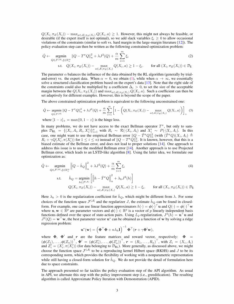
to avoid obstacles. We use an iRobot Create equipped with Kinect RGB-depth sensor and a laptop.We encode the Kinect observations with 1 × 3 grid cells (each 1m × 1m). The robot also has threebumpers to detect a collision from the front, left, and right. Figures 3a and 3b show a picture of therobot and its environment. In order to reach the goal, the robot needs to turn left to avoid a first boxand wall on the right, while not turning too much, to avoid the couch. Next, the robot must turnright to avoid a second box, but make sure not to turn too much or too soon to avoid colliding withthe wall or first box. Then, the robot needs to get into the hallway, turn right, and move forward toreach the goal position; the goal position is 6m forward and 1.5m right from the initial position.

The state space is represented by 3 non-negative integer features to represent number of point cloudsproduced by Kinect in each grid cell, and 2 continuous features (robot position). The robot has threediscrete actions: turn left, turn right, and move forward. The reward is minus the distance to thegoal, but if the robot’s front bumper is pressed and the robot moves forward, it receives a penaltyequal to 2 times the current distance to the goal. If the robot’s left bumper is pressed and the robotdoes not turn right, and vice-versa, it also receives 2 times the current distance to the goal. The robotoutputs actions at a rate of 1.7Hz.

We started from a single trajectory of demonstration, then incrementally added only RL data. Thenumber of data points added varied at each iteration, but the average was 160 data points, which isaround 1.6 minutes of exploration using -greedy exploration policy (decreasing over iterations).For 11 iterations, the training time was approximately 18 minutes. Initially, α

m was set to 0.9, thenit was decreased as new data was acquired. To evaluate the performance of each algorithm, we raneach iteration’s policy for a task horizon of 100 (≈ 1min); we repeated each iteration 5 times, tocompute the mean and standard deviation.

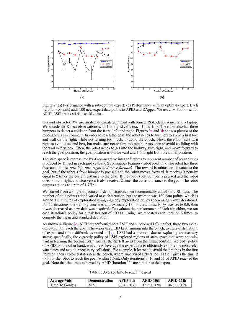
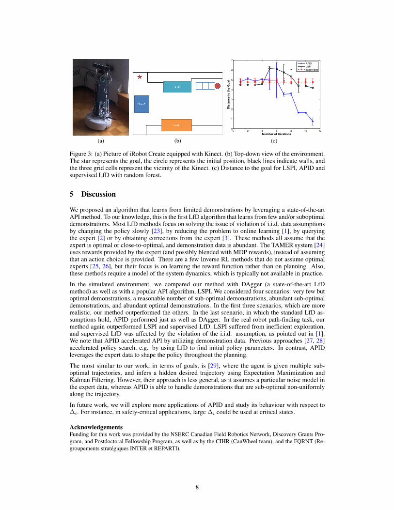
As shown in Figure 3c, APID outperformed both LSPI and supervised LfD; in fact, these two meth-ods could not reach the goal. The supervised LfD kept running into the couch, as state distributionsof expert and robot differed, as noted in [1]. LSPI had a problem due to exploring unnecessarystates; specifically, the -greedy policy of LSPI explored regions of state space that were not rele-vant in learning the optimal plan, such as the far left areas from the initial position. -greedy policyof APID, on the other hand, was able to leverage the expert data to efficiently explore the most rele-vant states and avoid unnecessary collisions. For example, it learned to avoid the first box in the firstiteration, then explored states near the couch, where supervised LfD failed. Table 1 gives the time ittook for the robot to reach the goal (within 1.5m). Only iterations 9, 10 and 11 of APID reached thegoal. Note that the times achieved by APID (iteration 11) are similar to the expert.

Table 1: Average time to reach the goal

Average Vals Demonstration APID-9th APID-10th APID-11th

Time To Goal(s) 35.9 38.4± 0.81 37.7± 0.84 36.1± 0.24

7

(a) (b)

0 2 4 6 8 10 120

1

2

3

4

5

6

7

Number of Iterations

Dis

tan

ce

to

th

e G

oa

l

APIDLSPIsupervised

(c)

Figure 3: (a) Picture of iRobot Create equipped with Kinect. (b) Top-down view of the environment.The star represents the goal, the circle represents the initial position, black lines indicate walls, andthe three grid cells represent the vicinity of the Kinect. (c) Distance to the goal for LSPI, APID andsupervised LfD with random forest.

5 Discussion

We proposed an algorithm that learns from limited demonstrations by leveraging a state-of-the-artAPI method. To our knowledge, this is the first LfD algorithm that learns from few and/or suboptimaldemonstrations. Most LfD methods focus on solving the issue of violation of i.i.d. data assumptionsby changing the policy slowly [23], by reducing the problem to online learning [1], by queryingthe expert [2] or by obtaining corrections from the expert [3]. These methods all assume that theexpert is optimal or close-to-optimal, and demonstration data is abundant. The TAMER system [24]uses rewards provided by the expert (and possibly blended with MDP rewards), instead of assumingthat an action choice is provided. There are a few Inverse RL methods that do not assume optimalexperts [25, 26], but their focus is on learning the reward function rather than on planning. Also,these methods require a model of the system dynamics, which is typically not available in practice.

In the simulated environment, we compared our method with DAgger (a state-of-the-art LfDmethod) as well as with a popular API algorithm, LSPI. We considered four scenarios: very few butoptimal demonstrations, a reasonable number of sub-optimal demonstrations, abundant sub-optimaldemonstrations, and abundant optimal demonstrations. In the first three scenarios, which are morerealistic, our method outperformed the others. In the last scenario, in which the standard LfD as-sumptions hold, APID performed just as well as DAgger. In the real robot path-finding task, ourmethod again outperformed LSPI and supervised LfD. LSPI suffered from inefficient exploration,and supervised LfD was affected by the violation of the i.i.d. assumption, as pointed out in [1].We note that APID accelerated API by utilizing demonstration data. Previous approaches [27, 28]accelerated policy search, e.g. by using LfD to find initial policy parameters. In contrast, APIDleverages the expert data to shape the policy throughout the planning.

The most similar to our work, in terms of goals, is [29], where the agent is given multiple sub-optimal trajectories, and infers a hidden desired trajectory using Expectation Maximization andKalman Filtering. However, their approach is less general, as it assumes a particular noise model inthe expert data, whereas APID is able to handle demonstrations that are sub-optimal non-uniformlyalong the trajectory.

In future work, we will explore more applications of APID and study its behaviour with respect to∆i. For instance, in safety-critical applications, large ∆i could be used at critical states.

Acknowledgements

Funding for this work was provided by the NSERC Canadian Field Robotics Network, Discovery Grants Pro-gram, and Postdoctoral Fellowship Program, as well as by the CIHR (CanWheel team), and the FQRNT (Re-groupements strategiques INTER et REPARTI).

8

References

[1] S. Ross, G. Gordon, and J. A. Bagnell. A reduction of imitation learning and structured prediction tono-regret online learning. In AISTATS, 2011. 1, 2, 6, 7, 8

[2] S. Chernova and M. Veloso. Interactive policy learning through confidence-based autonomy. Journal ofArtificial Intelligence Research, 34, 2009. 1, 8

[3] B. Argall, M. Veloso, and B. Browning. Teacher feedback to scaffold and refine demonstrated motionprimitives on a mobile robot. Robotics and Autonomous Systems, 59(3-4), 2011. 1, 8

[4] R. S. Sutton and A. G. Barto. Reinforcement Learning: An Introduction. MIT Press, 1998. 1[5] Cs. Szepesvari. Algorithms for Reinforcement Learning. Morgan Claypool Publishers, 2010. 1, 2[6] M. G. Lagoudakis and R. Parr. Least-squares policy iteration. Journal of Machine Learning Research, 4:

1107–1149, 2003. 2, 6[7] D. P. Bertsekas. Approximate policy iteration: A survey and some new methods. Journal of Control

Theory and Applications, 9(3):310–335, 2011. 2[8] A.-m. Farahmand, M. Ghavamzadeh, Cs. Szepesvari, and S. Mannor. Regularized policy iteration. In

NIPS 21, 2009. 2, 3[9] J. Z. Kolter and A. Y. Ng. Regularization and feature selection in least-squares temporal difference

learning. In ICML, 2009. 2[10] G. Taylor and R. Parr. Kernelized value function approximation for reinforcement learning. In ICML,

2009. 2[11] M. Ghavamzadeh, A. Lazaric, R. Munos, and M. Hoffman. Finite-sample analysis of Lasso-TD. In ICML,

2011. 2[12] I. Steinwart and A. Christmann. Support Vector Machines. Springer, 2008. 3, 5[13] I. Tsochantaridis, T. Joachims, T. Hofmann, Y. Altun, and Y. Singer. Large margin methods for structured

and interdependent output variables. Journal of Machine Learning Research, 6(2):1453–1484, 2006. 3[14] A. Antos, Cs. Szepesvari, and R. Munos. Learning near-optimal policies with Bellman-residual mini-

mization based fitted policy iteration and a single sample path. Machine Learning, 71:89–129, 2008.3

[15] A.-m. Farahmand and Cs. Szepesvari. Model selection in reinforcement learning. Machine Learning, 85(3):299–332, 2011. 4

[16] R. Munos. Error bounds for approximate policy iteration. In ICML, 2003. 4[17] A.-m. Farahmand, R. Munos, and Cs. Szepesvari. Error propagation for approximate policy and value

iteration. In NIPS 23, 2010. 4[18] B. Yu. Rates of convergence for empirical processes of stationary mixing sequences. The Annals of

Probability, 22(1):94–116, January 1994. 4[19] P.-M. Samson. Concentration of measure inequalities for Markov chains and φ-mixing processes. The

Annals of Probability, 28(1):416–461, 2000. 4[20] S. Boucheron, O. Bousquet, and G. Lugosi. Theory of classification: A survey of some recent advances.

ESAIM: Probability and Statistics, 9:323–375, 2005. 5[21] T. Hester, M. Quinlan, and P. Stone. RTMBA: A real-time model-based reinforcement learning architec-

ture for robot control. In ICRA, 2012. 5[22] CVX Research, Inc. CVX: Matlab software for disciplined convex programming, version 2.0. http:

//cvxr.com/cvx, August 2012. 5[23] S. Ross and J. A. Bagnell. Efficient reductions for imitation learning. In AISTATS, 2010. 8[24] W. B Knox and P. Stone. Reinforcement learning from simultaneous human and MDP reward. In AAMAS,

2012. 8[25] D. Ramachandran and E. Amir. Bayesian inverse reinforcement learning. In IJCAI, 2007. 8[26] B. D. Ziebart, A. Maas, J. A. Bagnell, and A. K. Dey. Maximum entropy inverse reinforcement learning.

In AAAI, 2008. 8[27] A. J. Ijspeert, J. Nakanishi, and S. Schaal. Learning attractor landscapes for learning motor primitives. In

NIPS 15, 2002. 8[28] J. Kober and J. Peters. Policy search for motor primitives in robotics. Machine Learning, 84(1-2):171–

203, 2011. 8[29] A. Coates, P. Abbeel, and A. Y. Ng. Learning for control from multiple demonstrations. In ICML, 2008.

8

9