Learning how antibodies are drafted and revised Frederick “Erick” Matsen Fred Hutchinson Cancer Research Center @ematsen http://matsen.fredhutch.org/ with Trevor Bedford (FH), Connor McCoy, Vladimir Minin (UW), and Duncan Ralph (FH)
Transcript
Learning how antibodies are drafted and revised
Frederick “Erick” Matsen
Fred Hutchinson Cancer Research Center
@ematsenhttp://matsen.fredhutch.org/
with Trevor Bedford (FH), Connor McCoy, Vladimir Minin (UW), and Duncan Ralph (FH)
RV144 HIV trial: 2003-200926,676 volunteers enrolled16,395 volunteers randomized125 infections$105,000,000 and 6 years
Prospective studies are expensive, slow, and entail complex moral issues.This does not lend itself to rapid vaccine development.
How might we guide vaccine development without disease exposure?
Vaccines manipulate the adaptive immune system
What can we learn from antibody-making B cells without battle-testing them through disease exposure?
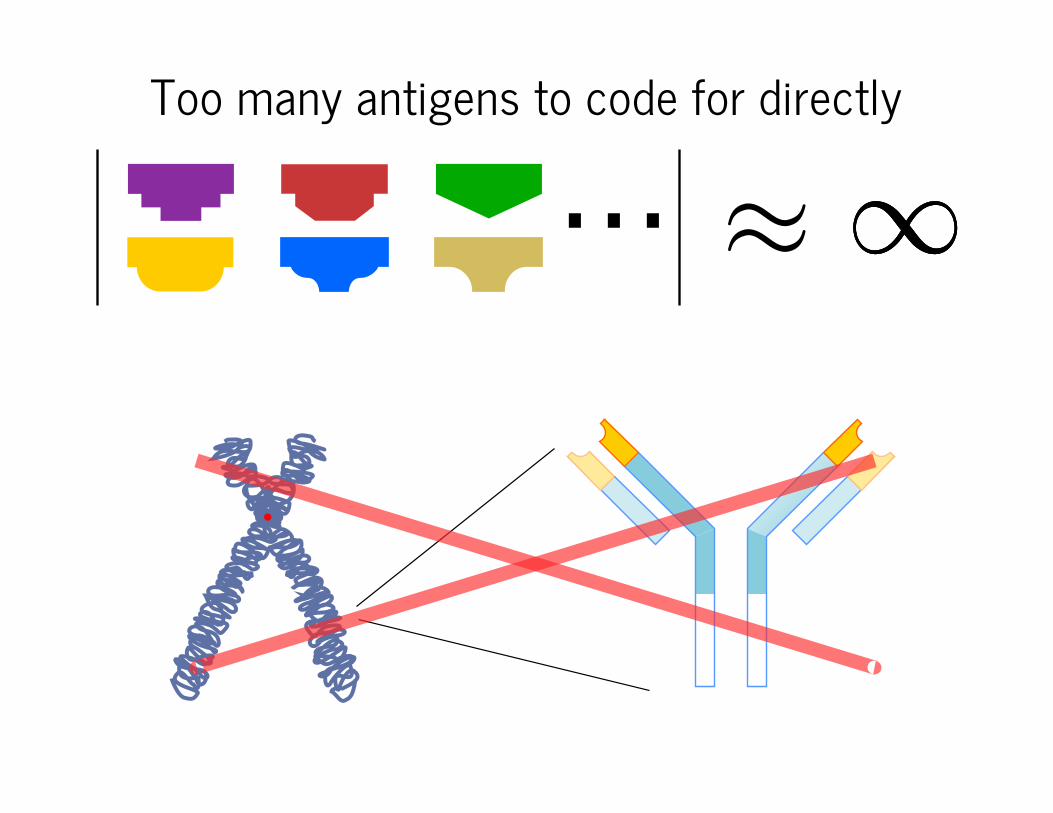
Antibodies bind antigensAntigen
Light chain
Heavy chain
Too many antigens to code for directly
≈∞⋯ ∞∞
B cell diversification processV genes D genes J genes
Affinitymaturation
Somatic hypermutation
VDJ rearrangement
includingerosion and
nontemplatedinsertion
AntigenNaive B cell
Experienced B cell
What germline really looks like (Eichler and Breden groups)
Big aim: reconstruct from memory reads
ACATGGCTC...
ATACGTTCC...
TTACGGTTC...
ATCCGGTAC...
ATACAGTCT...
...
reality
...inference
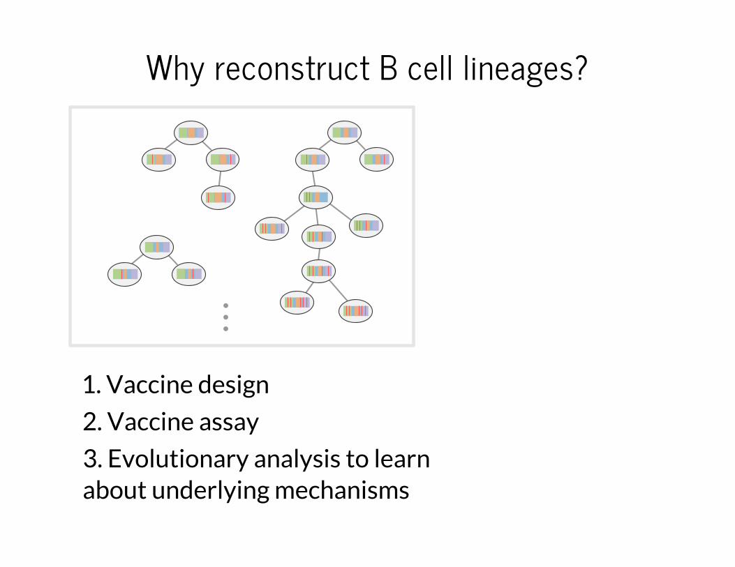
Why reconstruct B cell lineages?
...
1. Vaccine design
This one is really good.How can we elicit it?
Why reconstruct B cell lineages?
...
1. Vaccine design
immunogen 1
immunogen 2
Why reconstruct B cell lineages?
...
1. Vaccine design
?
2. Vaccine assay
Why reconstruct B cell lineages?
...
1. Vaccine design
3. Evolutionary analysis to learn about underlying mechanisms
2. Vaccine assay
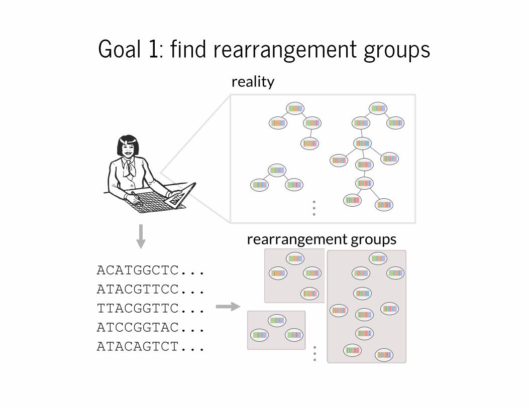
Goal 1: find rearrangement groups
ACATGGCTC...
ATACGTTCC...
TTACGGTTC...
ATCCGGTAC...
ATACAGTCT...
...
reality
...rearrangement groups
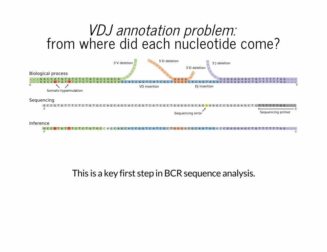
VDJ annotation problem: from where did each nucleotide come?
Somatic hypermutation
Sequencing primerSequencing error
3’V deletion
VD insertion
5’D deletion
3’D deletion5’J deletion
DJ insertion
Biological process
Sequencing
Inference
G
This is a key first step in BCR sequence analysis.
Data: Illumina reads from CDR3 locus
Somatic hypermut ation
Sequencing primerSequencing error
3’V deletion
VD insertion
5’D deletion
3’D deletion5’J deletion
DJ insertion
Biological process
SequencingG
Total of about 15 million unique 130nt sequences from memory B cellpopulations of three healthy individuals A, B, and C.
“Thread” reads onto structureV genes D genes J genes
...
...
...
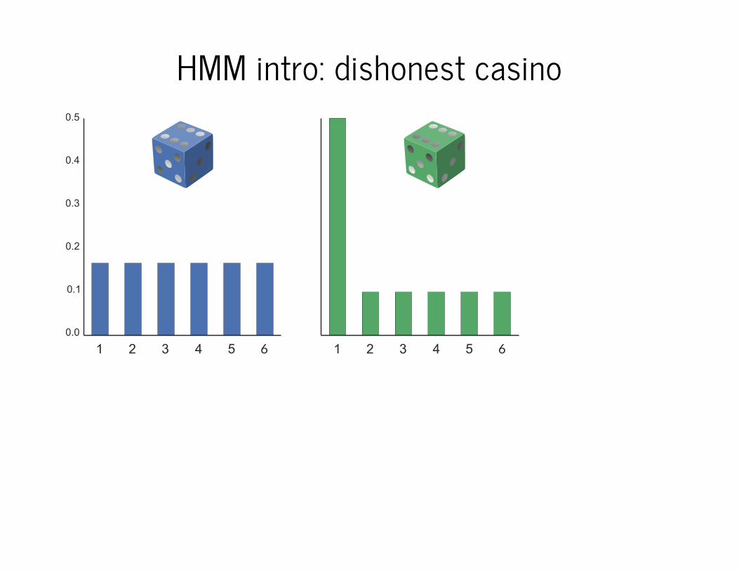
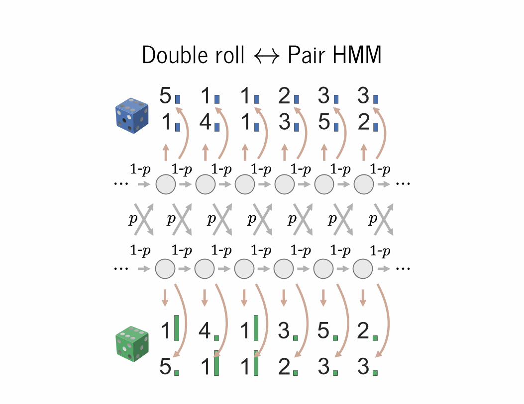
HMM intro: dishonest casino
6 6
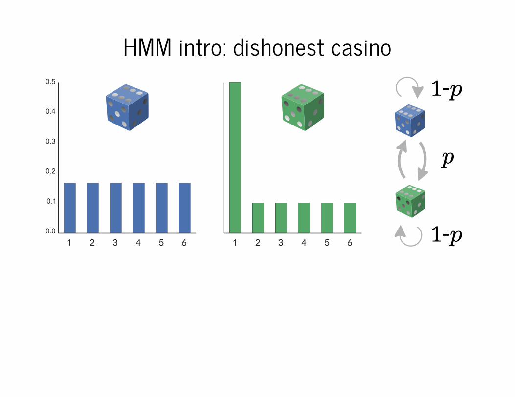
HMM intro: dishonest casino
6 6
1-p
1-p
p
HMM intro: dishonest casino
6 6
1-p
1-p
p
6 6
HMM intro: dishonest casino
6 6
1-p
1-p
p
6 6
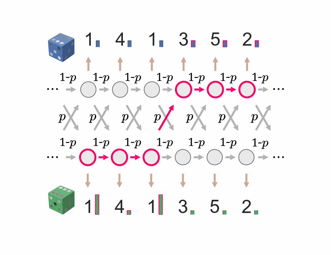
p1-p 1-p 1-p 1-p 1-p 1-p 1-p 1-p 1-p 1-p
p
1-p 1-p 1-p 1-p1-p
1-p 1-p 1-p 1-p1-p
p p p pp
1-p
1-p
p
...
...
...
...
1-p
1-p
p
1-p 1-p 1-p 1-p1-p
1-p 1-p 1-p 1-p1-p
p p p pp
1-p
1-p
p
...
...
...
...
1-p
1-p
V genes D genes J genes
...
...
...
V genes D genes J genes
...
...
...
V genes D genes J genes
...
...
...
Detour: write HMM inference package
We wanted to use HMMoC by G Lunter (Bioinf 2007)… then tried extending StochHMM by Lott & Korf (Bioinf 2014)…
but it ended up being a complete rewrite by Duncan to make ham.
Takes HMM description in concise & intuitive YAML format (for CpG example, 440 chars for ham vs 5,961 for HMMoC XML)slightly faster and more memory efficient than HMMoCcontinuous integration via Docker
Thank youTrevor Bedford, Connor McCoy, Vladimir Minin & Duncan RalphPhil Bradley for doing structural workMolecular work done by Paul Lindau in Phil Greenberg’s lab withsupport from Harlan Robins and Adaptive BiotechnologiesAdaptive Biotechnologies computational biology team
National Science Foundation and National Institute of HealthUniversity of Washington Center for AIDS Research (CFAR)University of Washington eScience InstituteW. M. Keck Foundation
Addenda
Measuring clustering agreementgood agreement:
bad agreement:
Cx
Cy
Cx
Cy
Intuition: “how much variability is there in the color for amongst theitems of a given color under ?
Cx
Cy
Mutual information IThink of cluster identity under for a uniformly selected point as a
random variable (similarly for and ):Cx
X Cy Y
I(X; Y ) = H(X) − H(X|Y )where is the entropy of (ignoring ), and is the
entropy of given the value for .H(X) X Y H(X|Y )
X Y
I(X; Y ) = p(x, y) log ( )∑y∈Y
∑x∈X
p(x, y)p(x) p(y)
AMI(U, V ) =MI(U, V ) − E{MI(U, V )}
max {H(U), H(V )} − E{MI(U, V )}
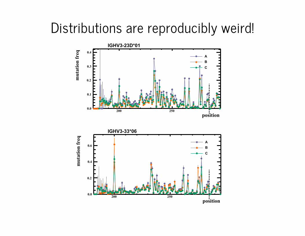
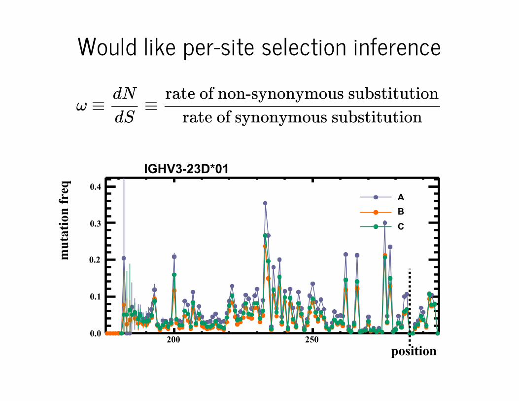
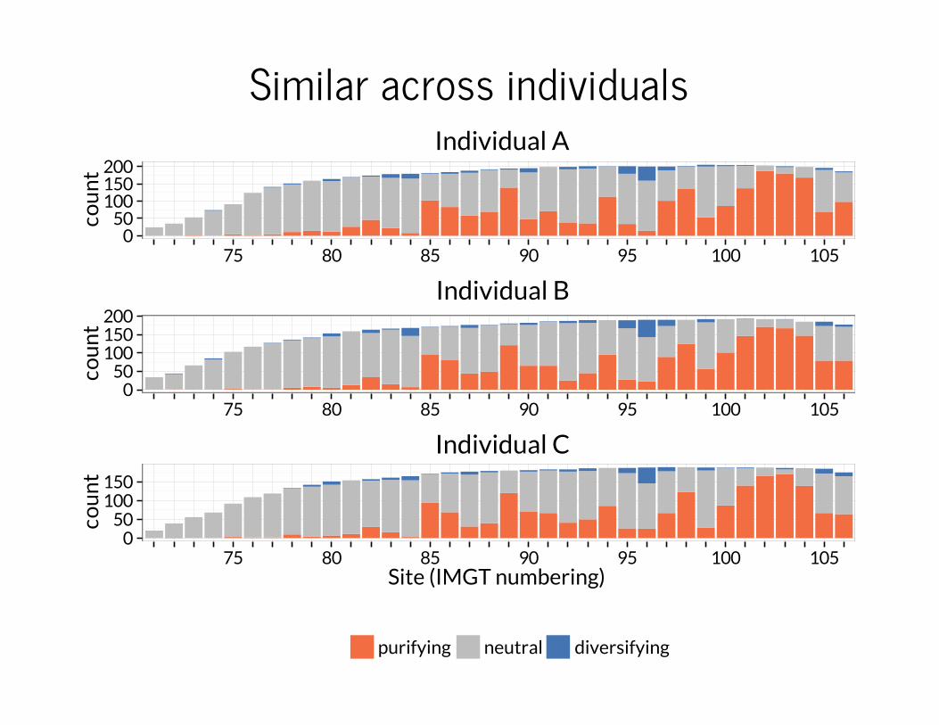
Estimates of the mutational process are quiteconsistent between individuals
(each point is a single entry for one of the matrices for a pair ofindividuals.)
Branch length differences between productive,unproductive
Unproductive rearrangements are more likely to be either: unchangedfrom germline, or more divergent.
Sites are generally under purifying selectionIndividual A
Individual B
Individual C
0
200
400
600
800
0
200
400
600
800
0
200
400
600
800
−1 0 1median log10(ω)
cou
nt
purifying diversifying neutral
cou
nt
cou
nt
Similar across individuals (ii)
Distribution of amino acidsbeginningof CDR3
selection for aromaticamino acids?Frequency: left of line = out-of-frame, right of line = in-frame
Stabilize with empirical Bayes regularizationAssume that , the substitution rate at site , comes from a Gamma
distribution with shape and rate :λl l
α β
∼ Gamma(α, β).λl
Model total substitution counts (sampled via stochastic mapping) for asite as Poisson with rate :λl
∼ Poisson( ),Cl λl
Fit and to all data, then draw rates from the posterior:α̂ β̂ λl
∣ ∼ Gamma( + , 1 + ).λl Cl Cl α̂ β̂
We extended this regularization to case of non-constant coverage.
Sequence countsstatus A B Cfunctional 4,139,983 4,861,800 3,748,306out-of-frame 533,919 794,845 558,246stop 104,525 169,423 112,901
Random factsMean length of D segment in individual A’s naive repertoire is 16.61.Subject A’s naive sequences were 37% CDR3Divergence between the various germ-line V genes:> summary(dist.dna(allele_01, pairwise.deletion=TRUE, model='raw'))Min. 1st Qu. Median Mean 3rd Qu. Max.0.003846 0.201300 0.344600 0.304700 0.384900 0.539500