Learning Loss for Active Learning

Donggeun Yoo1,2 and In So Kweon2

1Lunit Inc., Seoul, South Korea.2KAIST, Daejeon, South Korea.

dgyoo@lunit.io iskweon77@kaist.ac.kr

Abstract

The performance of deep neural networks improves with

more annotated data. The problem is that the budget for

annotation is limited. One solution to this is active learn-

ing, where a model asks human to annotate data that it

perceived as uncertain. A variety of recent methods have

been proposed to apply active learning to deep networks

but most of them are either designed specific for their tar-

get tasks or computationally inefficient for large networks.

In this paper, we propose a novel active learning method

that is simple but task-agnostic, and works efficiently with

the deep networks. We attach a small parametric module,

named “loss prediction module,” to a target network, and

learn it to predict target losses of unlabeled inputs. Then,

this module can suggest data that the target model is likely

to produce a wrong prediction. This method is task-agnostic

as networks are learned from a single loss regardless of tar-

get tasks. We rigorously validate our method through image

classification, object detection, and human pose estimation,

with the recent network architectures. The results demon-

strate that our method consistently outperforms the previ-

ous methods over the tasks.

1. Introduction

Data is flooding in, but deep neural networks are still

data-hungry. The empirical analysis of [33, 20] suggests

that the performance of recent deep networks is not yet

saturated with respect to the size of training data. For

this reason, learning methods from semi-supervised learn-

ing [42, 39, 33, 20] to unsupervised learning [1, 7, 58, 38]

are attracting attention along with weakly-labeled or unla-

beled large-scale data.

However, given a fixed amount of data, the performance

of the semi-supervised or unsupervised learning is still

bound to that of fully-supervised learning. The experimen-

Model

Loss prediction module

Input Target prediction

Loss prediction

(a) A model with a loss prediction module

.

.

Unlabeled

pool

⋯

Predicted

losses

Labeled

training set

Human oracles

annotate top-𝐾data points

(b) Active learning with a loss prediction module

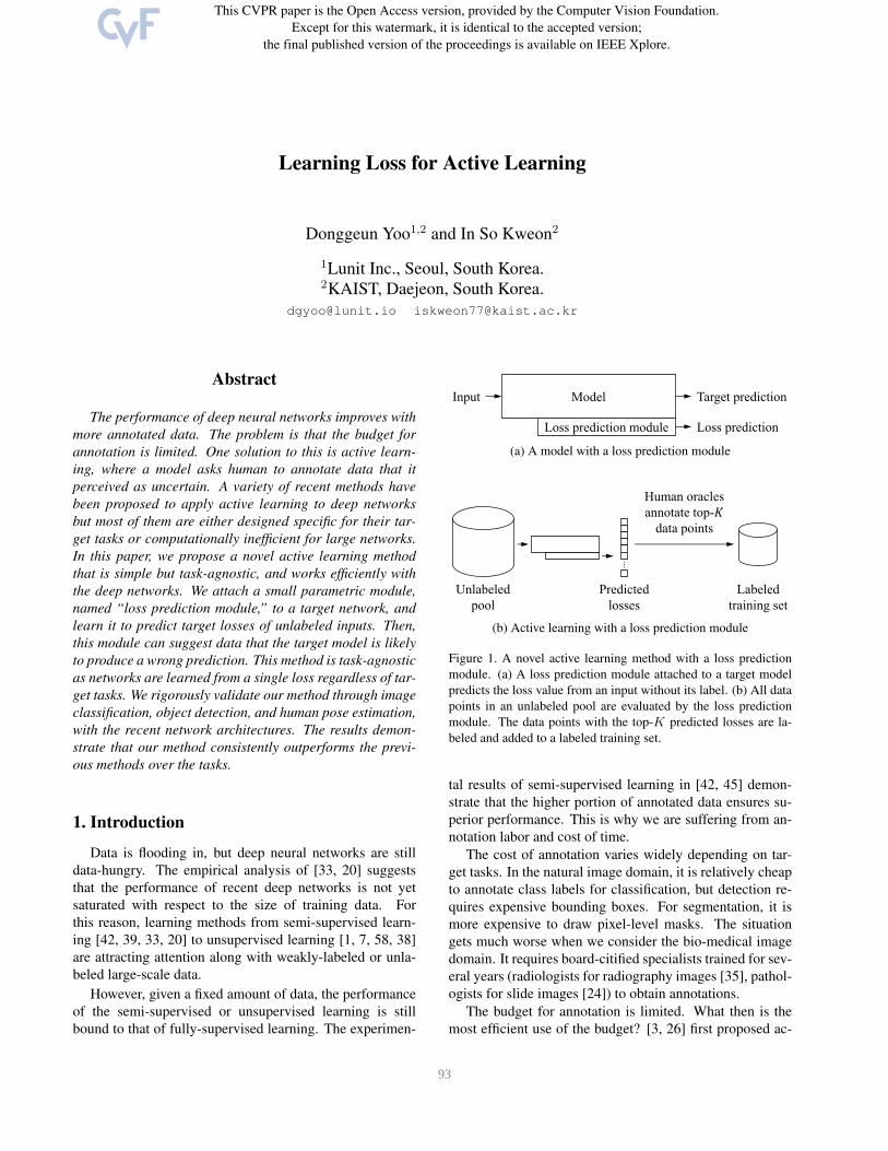
Figure 1. A novel active learning method with a loss prediction

module. (a) A loss prediction module attached to a target model

predicts the loss value from an input without its label. (b) All data

points in an unlabeled pool are evaluated by the loss prediction

module. The data points with the top-K predicted losses are la-

beled and added to a labeled training set.

tal results of semi-supervised learning in [42, 45] demon-

strate that the higher portion of annotated data ensures su-

perior performance. This is why we are suffering from an-

notation labor and cost of time.

The cost of annotation varies widely depending on tar-

get tasks. In the natural image domain, it is relatively cheap

to annotate class labels for classification, but detection re-

quires expensive bounding boxes. For segmentation, it is

more expensive to draw pixel-level masks. The situation

gets much worse when we consider the bio-medical image

domain. It requires board-citified specialists trained for sev-

eral years (radiologists for radiography images [35], pathol-

ogists for slide images [24]) to obtain annotations.

The budget for annotation is limited. What then is the

most efficient use of the budget? [3, 26] first proposed ac-

1 93

tive learning where a model actively selects data points that

the model is uncertain of. For an example of binary classifi-

cation [26], the data point whose posterior probability clos-

est to 0.5 is selected, annotated, and added to a training set.

The core idea of active learning is that the most informative

data point would be more beneficial to model improvement

than a randomly chosen data point.

Given a pool of unlabeled data, there have been three

major approaches according to the selection criteria: an

uncertainty-based approach, a diversity-based approach,

and expected model change. The uncertainty approach

[26, 19, 55, 52, 49, 4] defines and measures the quantity

of uncertainty to select uncertain data points, while the di-

versity approach [45, 37, 15, 5] selects diverse data points

that represent the whole distribution of the unlabeled pool.

Expected model change [44, 48, 12] selects data points that

would cause the greatest change to the current model pa-

rameters or outputs if we knew their labels. Readers can re-

view most of classical studies for these approaches in [46].

The simplest method of the uncertainty approach is to

utilize class posterior probabilities to define uncertainty.

The probability of a predicted class [26] or an entropy of

class posterior probabilities [19, 55] defines uncertainty of

a data point. Despite its simplicity, this approach has per-

formed remarkably well in various scenarios. For more

complex recognition tasks, it is required to re-define task-

specific uncertainty such as object detection [54], semantic

segmentation [29], and human pose estimation [8].

As a task-agnostic uncertainty approach, [49, 4] train

multiple models to construct a committee, and measure the

consensus between the multiple predictions from the com-

mittee. However, constructing a committee is too expen-

sive for current deep networks learned with large data. Re-

cently, Gal et al. [14] obtains uncertainty estimates from

deep networks through multiple forward passes by Monte

Carlo Dropout [13]. It was shown to be effective for clas-

sification with small datasets, but according to [45], it does

not scale to larger datasets.

The distribution approach could be task-agnostic as it

depends on a feature space, not on predictions. However,

extra engineering would be necessary to design a location-

invariant feature space for localization tasks such as object

detection and segmentation. The method of expected model

change has been successful for small models but it is com-

putationally impractical for recent deep networks.

The majority of empirical results from previous re-

searches suggest that active learning is actually reducing

the annotation cost. The problem is that most of methods

require task-specific design or are not efficient in the recent

deep networks, resulting in another engineering cost. In this

paper, we aim to propose a novel active learning method

that is simple but task-agnostic, and performs well on deep

networks.

A deep network is learned by minimizing a single loss,

regardless of what a task is, how many tasks there are, and

how complex an architecture is. This fact motivates our

task-agnostic design for active learning. If we can predict

the loss of a data point, it becomes possible to select data

points that are expected to have high losses. The selected

data points would be more informative to the current model.

To realize this scenario, we attach a “loss prediction

module” to a deep network and learn the module to predict

the loss of an input data point. The module is illustrated in

Figure 1-(a). Once the module is learned, it can be utilized

to active learning as shown in Figure 1-(b). We can apply

this method to any task that uses a deep network.

We validate the proposed method through image classi-

fication, human pose estimation, and object detection. The

human pose estimation is a typical regression task, and the

object detection is a more complex problem combined with

both regression and classification. The experimental results

demonstrate that the proposed method consistently outper-

forms previous methods with a current network architecture

for each recognition task. To the best of our knowledge,

this is the first work verified with three different recognition

tasks using the state-of-the-art deep network models.

1.1. Contributions

In summary, our major contributions are

1. Proposing a simple but efficient active learning method

with the loss prediction module, which is directly ap-

plicable to any tasks with recent deep networks.

2. Evaluating the proposed method with three learning

tasks including classification, regression, and a hybrid

of them, by using current network architectures.

2. Related Research

Active learning has advanced for more than a couple of

decades. First, we introduce classical active learning meth-

ods that use small-scale models [46]. In the uncertainty ap-

proach, a naive way to define uncertainty is to use the pos-

terior probability of a predicted class [26, 25], or the margin

between posterior probabilities of a predicted class and the

secondly predicted class [19, 43]. The entropy [47, 31, 19]

of class posterior probabilities generalizes the former def-

initions. For SVMs, distances [52, 53, 27] to the decision

boundaries can be used to define uncertainty. Another ap-

proach is the query-by-committee [49, 34, 18]. This method

constructs a committee comprising multiple independent

models, and measures disagreement among them to define

uncertainty.

The distribution approach chooses data points that rep-

resent the distribution of an unlabeled pool. The intuition is

that learning over a representative subset would be competi-

tive over the whole pool. To do so, [37] applies a clustering

94

algorithm to the pool, and [57, 9, 15] formulate the sub-

set selection as a discrete optimization problem. [5, 16, 32]

consider how close a data point is to surrounding data points

to choose one that could well propagate the knowledge. The

method of expected model change is a more sophisticated

and decision-theoretic approach for model improvement.

It utilizes the current model to estimate expected gradient

length [48], expected future errors [44], or expected output

changes [12, 21], to all possible labels.

Do these methods, advanced with small models and data,

well scale to large deep networks [23, 17] and data? Fortu-

nately, the uncertainty approach [28, 55] for classification

tasks still performs well despite its simplicity. However, a

task-specific design is necessary for other tasks since it uti-

lizes network outputs. As a more generalized uncertainty

approach, [14] obtains uncertainty estimates through mul-

tiple forward passes with Monte Carlo Dropout, but it is

computationally inefficient for recent large-scale learning as

it requires dense dropout layers that drastically slow down

the convergence speed. This method has been verified only

with small-scale classification tasks. [4] constructs a com-

mittee comprising 5 deep networks to measure disagree-

ment as uncertainty. It has shown the state-of-the-art clas-

sification performance, but it is also inefficient in terms of

memory and computation for large-scale problems.

Sener et al. [45] propose a distribution approach on an

intermediate feature space of a deep network. This method

is directly applicable to any task and network architec-

ture since it depends on intermediate features rather than

the task-specific outputs. However, it is still questionable

whether the intermediate feature representation is effective

for localization tasks such as detection and segmentation.

This method has also been verified only with classification

tasks. As the two approaches based on uncertainty and dis-

tribution are differently motivated, they are complementary

to each other. Thus, a variety of hybrid strategies have been

proposed [29, 59, 41, 56] for their specific tasks.

Our method can be categorized into the uncertainty ap-

proach but differs in that it predicts “loss” based on the in-

put contents, rather than statistically estimating uncertainty

from outputs. It is similar to a variety of hard example min-

ing [50, 11] since they regard training data points with high

losses as being significant for model improvement. How-

ever, ours is distinct from theirs in that we do not have an-

notations of data.

3. Method

In this section, we introduce the proposed active learn-

ing method. We start with an overview of the whole ac-

tive learning system in Section 3.1, and provide in-depth

descriptions of the loss prediction module in Section 3.2,

and the method to learn this module in Section 3.3.

3.1. Overview

In this section, we formally define the active learning

scenario with the proposed loss prediction module. In this

scenario, we have a set of models composed of a target

model Θtarget and a loss prediction module Θloss. The loss

prediction module is attached to the target model as illus-

trated in Figure 1-(a). The target model conducts the target

task as y = Θtarget(x), while the loss prediction module

predicts the loss l = Θloss(h). Here, h is a feature set of xextracted form several hidden layers of Θtarget.

In most real-world learning problems, we can gather a

large pool of unlabeled data UN at once. The subscript Ndenotes the number of data points. Then, we uniformly

sample K data points at random from the unlabeled pool,

and ask human oracles to annotate them to construct an ini-

tial labeled dataset L0K . The subscript 0 means it is the ini-

tial stage. This process reduces the size of the unlabeled

pool as U0N−K .

Once the initially labeled dataset L0K is obtained, we

jointly learn an initial target model Θ0target and an initial loss

prediction module Θ0loss. After initial training, we evaluate

all the data points in the unlabeled pool by the loss predic-

tion module to obtain data-loss pairs {(x, l)|x ∈ U0N−K}.

Then, human oracles annotate the data points of the K-

highest losses. The labeled dataset L0K is updated with them

and becomes L12K . After that, we learn the model set over

L12K to obtain {Θ1

target,Θ1loss}. This cycle, illustrated in Fig-

ure 1-(b), repeats until we meet a satisfactory performance

or until we have exhausted the budget for annotation.

3.2. Loss Prediction Module

The loss prediction module is core to our task-agnostic

active learning since it learns to imitate the loss defined in

the target model. This section describes how we design it.

The loss prediction module aims to minimize the engi-

neering cost of defining task-specific uncertainty for active

learning. Moreover, we also want to minimize the computa-

tional cost of learning the loss prediction module, as we are

already suffering from the computational cost of learning

very deep networks. To this end, we design a loss predic-

tion module that is (1) much smaller than the target model,

and (2) jointly learned with the target model. There is no

separated stage to learn this module.

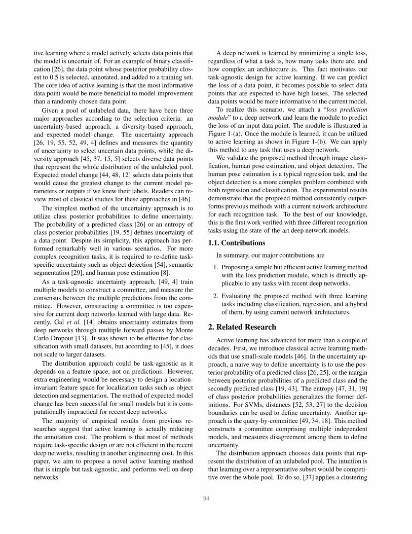
Figure 2 illustrates the architecture of our loss predic-

tion module. It takes multi-layer feature maps h as inputs

that are extracted between the mid-level blocks of the tar-

get model. These multiple connections let the loss predic-

tion module to choose necessary information between lay-

ers useful for loss prediction. Each feature map is reduced

to a fixed dimensional feature vector through a global aver-

age pooling (GAP) layer and a fully-connected layer. Then,

all features are concatenated and pass through another fully-

95

Target model

FC

GA

P

FC

ReL

U

GA

P

FC

ReL

U

GA

P

FC

ReL

ULoss

prediction

Mid-

block

Mid-

block

Mid-

block

Output

block

Target

prediction

Concat.

Figure 2. The architecture of the loss prediction module. This

module is connected to several layers of the target model to take

multi-level knowledge into consideration for loss prediction. The

multi-level features are fused and map to a scalar value as the loss

prediction.

connected layer, resulting in a scalar value l as a predicted

loss. Learning this two-story module requires much less

memory and computation than the target model. We have

tried to make this module deeper and wider, but the perfor-

mance does not change much.

3.3. Learning Loss

In this section, we provide an in-detail description of

how to learn the loss prediction module defined before. Let

us suppose we start the s-th active learning stage. We have

a labeled dataset LsK·(s+1) and a model set composed of a

target model Θtarget and a loss prediction module Θloss. Our

objective is to learn the model set for this stage s to obtain

{Θstarget,Θ

sloss}.

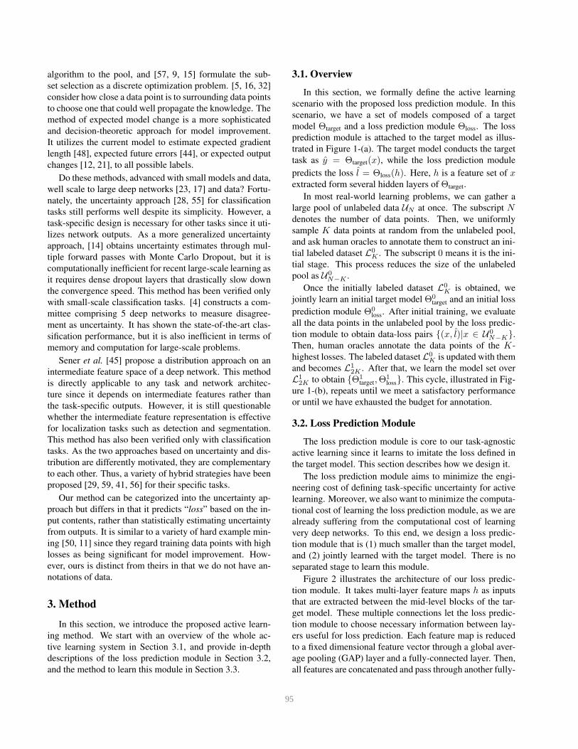
Given a training data point x, we obtain a target pre-

diction through the target model as y = Θtarget(x), and

also a predicted loss through the loss prediction module as

l = Θloss(h). With the target annotation y of x, the target

loss can be computed as l = Ltarget(y, y) to learn the tar-

get model. Since this loss l is a ground-truth target of h for

the loss prediction module, we can also compute the loss

for the loss prediction module as Lloss(l, l). Then, the final

loss function to jointly learn both of the target model and

the loss prediction module is defined as

Ltarget(y, y) + λ · Lloss(l, l) (1)

where λ is a scaling constant. This procedure to define the

final loss is illustrated in Figure 3.

Perhaps the simplest way to define the loss-prediction

loss function is the mean square error (MSE) Lloss(l, l) =

(l − l)2. However, MSE is not a suitable choice for this

problem since the scale of the real loss l changes (decreases

in overall) as learning of the target model progresses. Min-

imizing MSE would let the loss prediction module adapt

roughly to the scale changes of the loss l, rather than fit-

ting to the exact value. We have tried to minimize MSE

but failed to learn a good loss prediction module, and ac-

tive learning with this module actually demonstrates perfor-

mance worse than previous methods.

Model

Loss prediction module

InputTarget

prediction

Loss

prediction

Target

GT

Target

loss

Loss-prediction

loss

Figure 3. Method to learn the loss. Given an input, the target model

outputs a target prediction, and the loss prediction module outputs

a predicted loss. The target prediction and the target annotation are

used to compute a target loss to learn the target model. Then, the

target loss is regarded as a ground-truth loss for the loss prediction

module, and used to compute the loss-prediction loss.

It is necessary for the loss-prediction loss function to dis-

card the overall scale of l. Our solution is to compare a

pair of samples. Let us consider a training iteration with a

mini-batch Bs ⊂ LsK·(s+1). In the mini-batch whose size is

B, we can make B/2 data pairs such as {xp = (xi, xj)}.

The subscript p represents that it is a pair, and the mini-

batch size B should be an even number. Then, we can learn

the loss prediction module by considering the difference be-

tween a pair of loss predictions, which completely make the

loss prediction module discard the overall scale changes. To

this end, the loss function for the loss prediction module is

defined as

Lloss(lp, lp) = max

(

0,−✶(li, lj) · (li − lj) + ξ)

s.t. ✶(li, lj) =

{

+1, if li > lj

−1, otherwise(2)

where ξ is a pre-defined positive margin and the subscript palso represents the pair of (i, j). For instance when li > lj ,

this function states that no loss is given to the module only

if li is larger than lj + ξ, but otherwise a loss is given to the

module to force it to increase li and decrease lj .

Given a mini-batch Bs in the active learning stage s, our

final loss function to jointly learn the target model and the

loss prediction module is

1

B

∑

(x,y)∈Bs

Ltarget(y, y) + λ2

B·

∑

(xp,yp)∈Bs

Lloss(lp, lp)

s.t.

y = Θtarget(x)

lp = Θloss(hp)

lp = Ltarget(yp, yp).

(3)

Minimizing this final loss give us Θsloss as well as Θs

target

without any separated learning procedure nor any task-

specific assumption. The learning process is efficient as the

loss prediction module Θsloss has been designed to contain

96

a small number of parameters but to utilize rich mid-level

representations h of the target model. This loss prediction

module will pick the most informative data points and ask

human oracles to annotate them for the next active learning

stage s+ 1.

4. Evaluation

In this section, we rigorously evaluate our method

through three visual recognition tasks. To verify whether

our method works efficiently regardless of tasks, we choose

diverse target tasks including image classification as a clas-

sification task, object detection as a hybrid task of classifica-

tion and regression, and human pose estimation as a typical

regression problem. These three tasks are indeed important

research topics for visual recognition in computer vision,

and are very useful for many real-world applications.

We have implemented our method and all the recogni-

tion tasks with PyTorch [40]. For all tasks, we initialize a

labeled dataset L0K by randomly sampling K=1,000 data

points from the entire dataset UN . In each active learn-

ing cycle, we continue to train the current model by adding

K=1,000 labeled data points. The margin ξ defined in the

loss function (Equation 2) is set to 1. We design the fully-

connected layers (FCs) in Figure 2 except for the last one to

produce a 128-dimensional feature. For each active learning

method, we repeat the same experiment multiple times with

different initial labeled datasets, and report the performance

mean and standard deviation. For each trial, our method

and compared methods share the same random seed for a

fair comparison. Other implementation details, datasets,

and experimental results for each task are described in the

following Sections 4.1, 4.2, 4.3.

4.1. Image Classification

Image classification is a common problem that has been

verified by most of the previous active learning methods. In

this problem, a target model recognizes the category of a

major object from an input image, so object category labels

are required for supervised learning.

Dataset We choose CIFAR-10 dataset [22] as it has been

used for recent active learning methods [45, 4]. CIFAR-10

consists of 60,000 images of 32×32×3 size, assigned with

one of 10 object categories. The training and test sets con-

tain 50,000 and 10,000 images respectively. We regard the

training set as the initial unlabeled pool U50,000. As studied

in [45, 46], selecting K-most uncertain samples from such

a large pool U50,000 often does not work well, because image

contents among the K samples are overlapped. To address

this, [4] obtains a random subset SM ⊂ UN for each active

learning stage and choose K-most uncertain samples from

SM . We adopt this simple yet efficient scheme and set the

subset size to M=10,000. As an evaluation metric, we use

the classification accuracy.

Target model We employ the 18-layer residual network

(ResNet-18) [17] as we aim to verify our method with cur-

rent deep architectures. We have utilized an open source1

in which this model specified for CIFAR showing 93.02%

accuracy is implemented. ResNet-18 for CIFAR is identi-

cal to the original ResNet-18 except for the first convolution

and pooling layers. The first convolution layer is changed

to contain 3×3 kernels with the stride of 1 and the padding

of 1, and the max pooling layer is dropped, to adapt to the

small size images of CIFAR.

Loss prediction module ResNet-18 is composed of 4 ba-

sic blocks {convi 1, convi 2 | i=2, 3, 4, 5} following the

first convolution layer. Each block comprises two convolu-

tion layers. We simply connect the loss prediction module

to each of the basic blocks to utilize the 4 rich features from

the blocks for estimating the loss.

Learning For training, we apply a standard augmentation

scheme including 32×32 size random crop from 36×36

zero-padded images and random horizontal flip, and nor-

malize images using the channel mean and standard devi-

ation vectors estimated over the training set. For each of

active learning cycle, we learn the model set {Θstarget,Θ

sloss}

for 200 epochs with the mini-batch size of 128 and the ini-

tial learning rate of 0.1. After 160 epochs, we decrease the

learning rate to 0.01. The momentum and the weight decay

are 0.9 and 0.0005 respectively. After 120 epochs, we stop

the gradient from the loss prediction module propagated to

the target model. We set λ that scales the loss-prediction

loss in Equation 3 to 1.

Comparison targets We compare our method with ran-

dom sampling, entropy-based sampling [47, 31], and core-

set sampling [45], which is a recent distribution approach.

For the entropy-based method, we compute the entropy

from a softmax output vector. For core-set, we have im-

plemented K-Center-Greedy algorithm in [45] since it is

simple to implement yet marginally worse than the mixed

integer program. We also run the algorithm over the last

feature space right before the classification layer as [45] do.

Note that we use exactly the same hyper-parameters to train

target models for all methods including ours.

The results are shown in Figure 4. Each point is an aver-

age of 5 trials with different initial labeled datasets. Our

implementations show that both entropy-based and core-

set methods have better results than the random baseline.

In the last active learning cycle, the entropy and core-set

1https://github.com/kuangliu/pytorch-cifar

97

1k 2k 3k 4k 5k 6k 7k 8k 9k 10kNumber of labeled images

0.5

0.6

0.7

0.8

0.9

Acc

urac

y (m

ean

of 5

tria

ls)

random meanrandom mean±stdentropy meanentropy mean±stdcore-set meancore-set mean±stdlearn loss mse meanlearn loss mse mean±stdlearn loss meanlearn loss mean±std

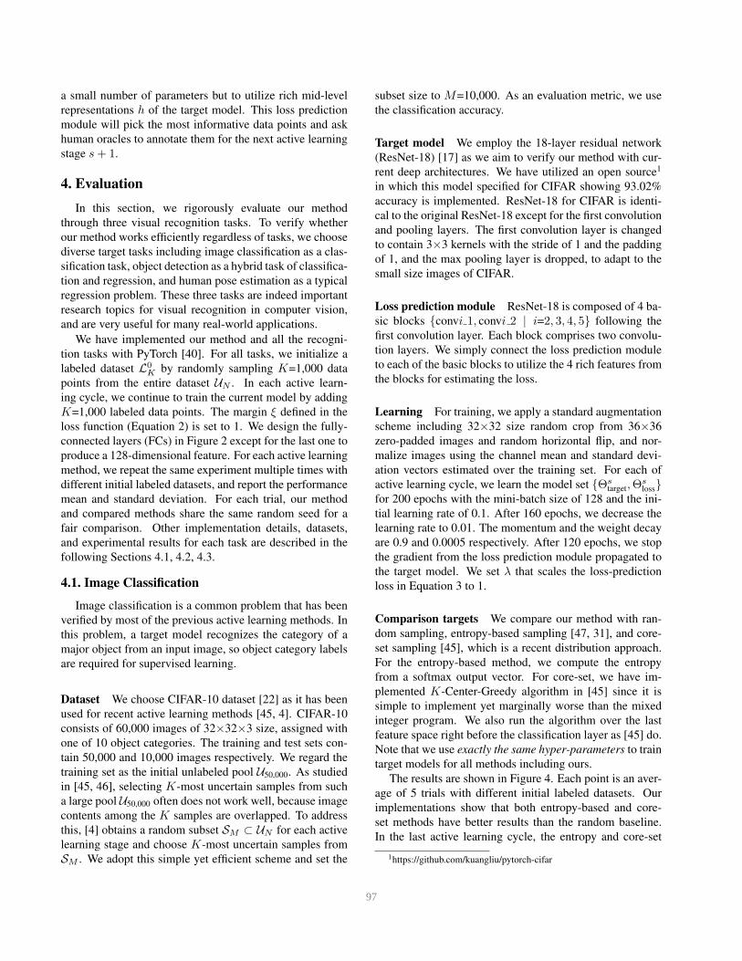
Figure 4. Active learning results of image classification over

CIFAR-10.

methods show 0.9059 and 0.9010 respectively, while the

random baseline shows 0.8764. The performance gaps be-

tween these methods are similar to those of [4]. In particu-

lar, the simple entropy-based method works very effectively

with the classification which is typically learned to mini-

mize cross-entropy between predictions and target labels.

Our method noted as “learn loss” shows the highest per-

formance for all active learning cycles. In the last cy-

cle, our method achieves an accuracy of 0.9101. This is

0.42% higher than the entropy method and 0.91% higher

than the core-set method. Although the performance gap

to the entropy-based method is marginal in classification,

our method can be effectively applied to more complex and

diverse target tasks.

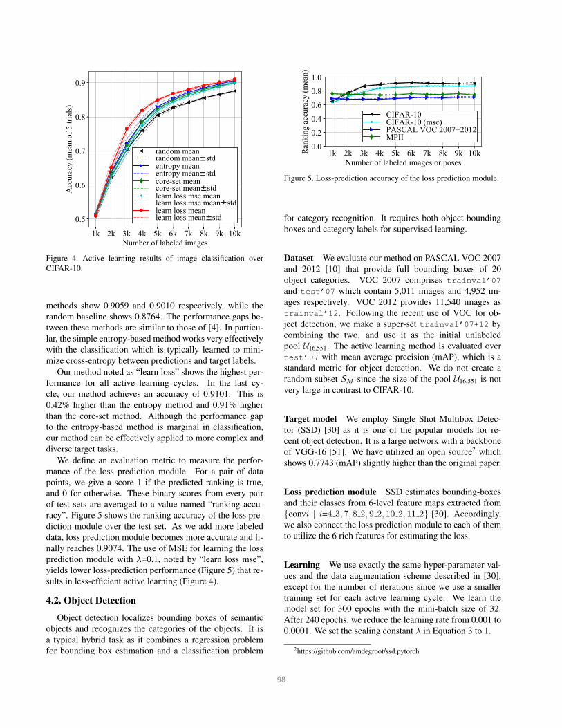
We define an evaluation metric to measure the perfor-

mance of the loss prediction module. For a pair of data

points, we give a score 1 if the predicted ranking is true,

and 0 for otherwise. These binary scores from every pair

of test sets are averaged to a value named “ranking accu-

racy”. Figure 5 shows the ranking accuracy of the loss pre-

diction module over the test set. As we add more labeled

data, loss prediction module becomes more accurate and fi-

nally reaches 0.9074. The use of MSE for learning the loss

prediction module with λ=0.1, noted by “learn loss mse”,

yields lower loss-prediction performance (Figure 5) that re-

sults in less-efficient active learning (Figure 4).

4.2. Object Detection

Object detection localizes bounding boxes of semantic

objects and recognizes the categories of the objects. It is

a typical hybrid task as it combines a regression problem

for bounding box estimation and a classification problem

1k 2k 3k 4k 5k 6k 7k 8k 9k 10kNumber of labeled images or poses

0.0

0.2

0.4

0.6

0.8

1.0

Ran

king

acc

urac

y (m

ean)

CIFAR-10CIFAR-10 (mse)PASCAL VOC 2007+2012MPII

Figure 5. Loss-prediction accuracy of the loss prediction module.

for category recognition. It requires both object bounding

boxes and category labels for supervised learning.

Dataset We evaluate our method on PASCAL VOC 2007

and 2012 [10] that provide full bounding boxes of 20

object categories. VOC 2007 comprises trainval’07

and test’07 which contain 5,011 images and 4,952 im-

ages respectively. VOC 2012 provides 11,540 images as

trainval’12. Following the recent use of VOC for ob-

ject detection, we make a super-set trainval’07+12 by

combining the two, and use it as the initial unlabeled

pool U16,551. The active learning method is evaluated over

test’07 with mean average precision (mAP), which is a

standard metric for object detection. We do not create a

random subset SM since the size of the pool U16,551 is not

very large in contrast to CIFAR-10.

Target model We employ Single Shot Multibox Detec-

tor (SSD) [30] as it is one of the popular models for re-

cent object detection. It is a large network with a backbone

of VGG-16 [51]. We have utilized an open source2 which

shows 0.7743 (mAP) slightly higher than the original paper.

Loss prediction module SSD estimates bounding-boxes

and their classes from 6-level feature maps extracted from

{convi | i=4 3, 7, 8 2, 9 2, 10 2, 11 2} [30]. Accordingly,

we also connect the loss prediction module to each of them

to utilize the 6 rich features for estimating the loss.

Learning We use exactly the same hyper-parameter val-

ues and the data augmentation scheme described in [30],

except for the number of iterations since we use a smaller

training set for each active learning cycle. We learn the

model set for 300 epochs with the mini-batch size of 32.

After 240 epochs, we reduce the learning rate from 0.001 to

0.0001. We set the scaling constant λ in Equation 3 to 1.

2https://github.com/amdegroot/ssd.pytorch

98

1k 2k 3k 4k 5k 6k 7k 8k 9k 10kNumber of labeled images

0.55

0.60

0.65

0.70

mA

P (m

ean

of 3

tria

ls)

random meanrandom mean±stdentropy meanentropy mean±stdcore-set meancore-set mean±stdlearn loss meanlearn loss mean±std

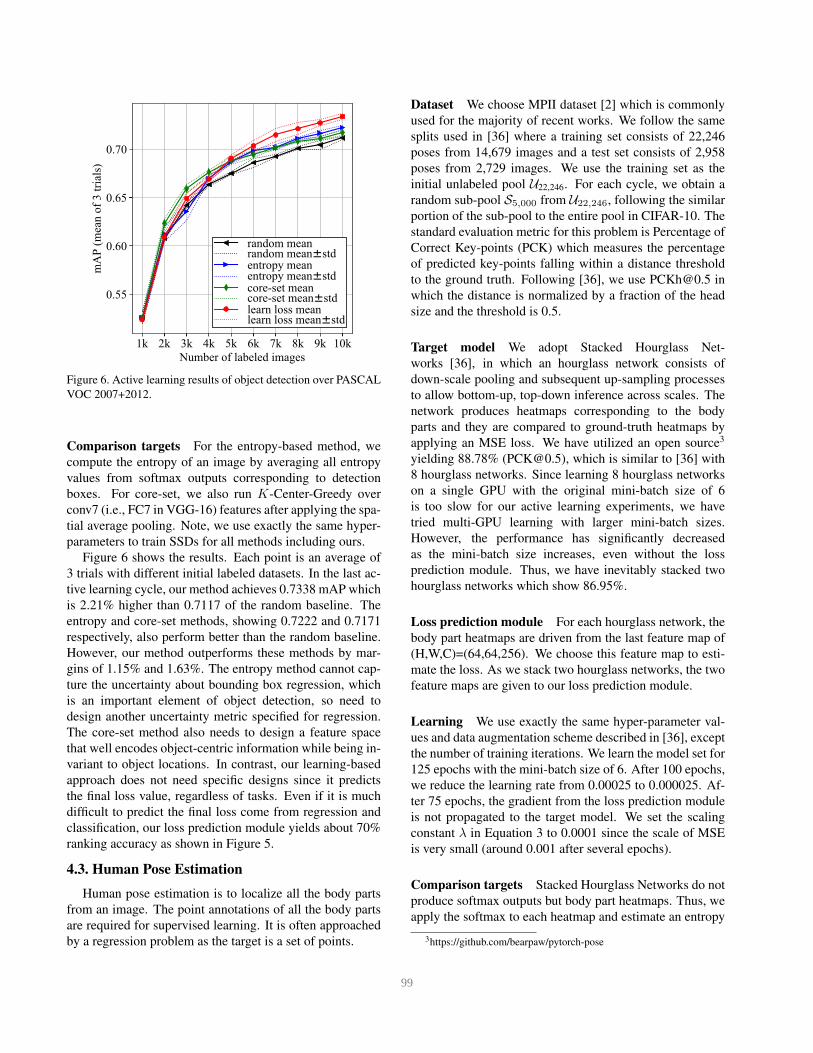
Figure 6. Active learning results of object detection over PASCAL

VOC 2007+2012.

Comparison targets For the entropy-based method, we

compute the entropy of an image by averaging all entropy

values from softmax outputs corresponding to detection

boxes. For core-set, we also run K-Center-Greedy over

conv7 (i.e., FC7 in VGG-16) features after applying the spa-

tial average pooling. Note, we use exactly the same hyper-

parameters to train SSDs for all methods including ours.

Figure 6 shows the results. Each point is an average of

3 trials with different initial labeled datasets. In the last ac-

tive learning cycle, our method achieves 0.7338 mAP which

is 2.21% higher than 0.7117 of the random baseline. The

entropy and core-set methods, showing 0.7222 and 0.7171

respectively, also perform better than the random baseline.

However, our method outperforms these methods by mar-

gins of 1.15% and 1.63%. The entropy method cannot cap-

ture the uncertainty about bounding box regression, which

is an important element of object detection, so need to

design another uncertainty metric specified for regression.

The core-set method also needs to design a feature space

that well encodes object-centric information while being in-

variant to object locations. In contrast, our learning-based

approach does not need specific designs since it predicts

the final loss value, regardless of tasks. Even if it is much

difficult to predict the final loss come from regression and

classification, our loss prediction module yields about 70%

ranking accuracy as shown in Figure 5.

4.3. Human Pose Estimation

Human pose estimation is to localize all the body parts

from an image. The point annotations of all the body parts

are required for supervised learning. It is often approached

by a regression problem as the target is a set of points.

Dataset We choose MPII dataset [2] which is commonly

used for the majority of recent works. We follow the same

splits used in [36] where a training set consists of 22,246

poses from 14,679 images and a test set consists of 2,958

poses from 2,729 images. We use the training set as the

initial unlabeled pool U22,246. For each cycle, we obtain a

random sub-pool S5,000 from U22,246, following the similar

portion of the sub-pool to the entire pool in CIFAR-10. The

standard evaluation metric for this problem is Percentage of

Correct Key-points (PCK) which measures the percentage

of predicted key-points falling within a distance threshold

to the ground truth. Following [36], we use PCKh@0.5 in

which the distance is normalized by a fraction of the head

size and the threshold is 0.5.

Target model We adopt Stacked Hourglass Net-

works [36], in which an hourglass network consists of

down-scale pooling and subsequent up-sampling processes

to allow bottom-up, top-down inference across scales. The

network produces heatmaps corresponding to the body

parts and they are compared to ground-truth heatmaps by

applying an MSE loss. We have utilized an open source3

yielding 88.78% (PCK@0.5), which is similar to [36] with

8 hourglass networks. Since learning 8 hourglass networks

on a single GPU with the original mini-batch size of 6

is too slow for our active learning experiments, we have

tried multi-GPU learning with larger mini-batch sizes.

However, the performance has significantly decreased

as the mini-batch size increases, even without the loss

prediction module. Thus, we have inevitably stacked two

hourglass networks which show 86.95%.

Loss prediction module For each hourglass network, the

body part heatmaps are driven from the last feature map of

(H,W,C)=(64,64,256). We choose this feature map to esti-

mate the loss. As we stack two hourglass networks, the two

feature maps are given to our loss prediction module.

Learning We use exactly the same hyper-parameter val-

ues and data augmentation scheme described in [36], except

the number of training iterations. We learn the model set for

125 epochs with the mini-batch size of 6. After 100 epochs,

we reduce the learning rate from 0.00025 to 0.000025. Af-

ter 75 epochs, the gradient from the loss prediction module

is not propagated to the target model. We set the scaling

constant λ in Equation 3 to 0.0001 since the scale of MSE

is very small (around 0.001 after several epochs).

Comparison targets Stacked Hourglass Networks do not

produce softmax outputs but body part heatmaps. Thus, we

apply the softmax to each heatmap and estimate an entropy

3https://github.com/bearpaw/pytorch-pose

99

1k 2k 3k 4k 5k 6k 7k 8k 9k 10kNumber of labeled poses

0.60

0.65

0.70

0.75

0.80

PCK

h@0.

5 (m

ean

of 3

tria

ls)

random meanrandom mean±stdentropy meanentropy mean±stdcore-set meancore-set mean±stdlearn loss meanlearn loss mean±std

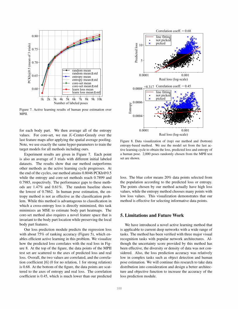
Figure 7. Active learning results of human pose estimation over

MPII.

for each body part. We then average all of the entropy

values. For core-set, we run K-Center-Greedy over the

last feature maps after applying the spatial average pooling.

Note, we use exactly the same hyper-parameters to train the

target models for all methods including ours.

Experiment results are given in Figure 7. Each point

is also an average of 3 trials with different initial labeled

datasets. The results show that our method outperforms

other methods as the active learning cycle progresses. At

the end of the cycles, our method attains 0.8046 PCKh@0.5

while the entropy and core-set methods reach 0.7899 and

0.7985, respectively. The performance gaps to these meth-

ods are 1.47% and 0.61%. The random baseline shows

the lowest of 0.7862. In human pose estimation, the en-

tropy method is not as effective as the classification prob-

lem. While this method is advantageous to classification in

which a cross-entropy loss is directly minimized, this task

minimizes an MSE to estimate body part heatmaps. The

core-set method also requires a novel feature space that is

invariant to the body part location while preserving the local

body part features.

Our loss prediction module predicts the regression loss

with about 75% of ranking accuracy (Figure 5), which en-

ables efficient active learning in this problem. We visualize

how the predicted loss correlates with the real loss in Fig-

ure 8. At the top of the figure, the data points of the MPII

test set are scattered to the axes of predicted loss and real

loss. Overall, the two values are correlated, and the correla-

tion coefficient [6] (0 for no relation, 1 for strong relation)

is 0.68. At the bottom of the figure, the data points are scat-

tered to the axes of entropy and real loss. The correlation

coefficient is 0.45, which is much lower than our predicted

0.0001 0.001Real loss (log-scale)

5

10

Pred

icte

d lo

ss

Correlation coeff. = 0.68

line fittingnot pickedpicked

0.0001 0.001Real loss (log-scale)

0.0004

0.0006

0.0008

Entro

py

+8.317 Correlation coeff. = 0.45

line fittingnot pickedpicked

Figure 8. Data visualization of (top) our method and (bottom)

entropy-based method. We use the model set from the last ac-

tive learning cycle to obtain the loss, predicted loss and entropy of

a human pose. 2,000 poses randomly chosen from the MPII test

set are shown.

loss. The blue color means 20% data points selected from

the population according to the predicted loss or entropy.

The points chosen by our method actually have high loss

values, while the entropy method chooses many points with

low loss values. This visualization demonstrates that our

method is effective for selecting informative data points.

5. Limitations and Future Work

We have introduced a novel active learning method that

is applicable to current deep networks with a wide range of

tasks. The method has been verified with three major visual

recognition tasks with popular network architectures. Al-

though the uncertainty score provided by this method has

been effective, the diversity or density of data was not con-

sidered. Also, the loss prediction accuracy was relatively

low in complex tasks such as object detection and human

pose estimation. We will continue this research to take data

distribution into consideration and design a better architec-

ture and objective function to increase the accuracy of the

loss prediction module.

100

References

[1] P. Agrawal, J. Carreira, and J. Malik. Learning to see by

moving. In Proceedings of the IEEE International Confer-

ence on Computer Vision, pages 37–45, 2015.

[2] M. Andriluka, L. Pishchulin, P. Gehler, and B. Schiele. 2d

human pose estimation: New benchmark and state of the

art analysis. In Proceedings of the IEEE Conference on

computer Vision and Pattern Recognition, pages 3686–3693,

2014.

[3] L. E. Atlas, D. A. Cohn, and R. E. Ladner. Training con-

nectionist networks with queries and selective sampling. In

Advances in neural information processing systems, pages

566–573, 1990.

[4] W. H. Beluch, T. Genewein, A. Nurnberger, and J. M. Kohler.

The power of ensembles for active learning in image classifi-

cation. In Proceedings of the IEEE Conference on Computer

Vision and Pattern Recognition, pages 9368–9377, 2018.

[5] M. Bilgic and L. Getoor. Link-based active learning. In

NIPS Workshop on Analyzing Networks and Learning with

Graphs, 2009.

[6] R. Boddy and G. Smith. Statistical methods in practice: for

scientists and technologists. John Wiley & Sons, 2009.

[7] C. Doersch, A. Gupta, and A. A. Efros. Unsupervised vi-

sual representation learning by context prediction. In Pro-

ceedings of the IEEE International Conference on Computer

Vision, pages 1422–1430, 2015.

[8] S. Dutt Jain and K. Grauman. Active image segmenta-

tion propagation. In Proceedings of the IEEE Conference

on Computer Vision and Pattern Recognition, pages 2864–

2873, 2016.

[9] E. Elhamifar, G. Sapiro, A. Yang, and S. Shankar Sasrty. A

convex optimization framework for active learning. In Pro-

ceedings of the IEEE International Conference on Computer

Vision, pages 209–216, 2013.

[10] M. Everingham, L. Van Gool, C. K. I. Williams, J. Winn, and

A. Zisserman. The pascal visual object classes (voc) chal-

lenge. International Journal of Computer Vision, 88(2):303–

338, June 2010.

[11] P. F. Felzenszwalb, R. B. Girshick, D. McAllester, and D. Ra-

manan. Object detection with discriminatively trained part-

based models. IEEE transactions on pattern analysis and

machine intelligence, 32(9):1627–1645, 2010.

[12] A. Freytag, E. Rodner, and J. Denzler. Selecting influen-

tial examples: Active learning with expected model out-

put changes. In European Conference on Computer Vision,

pages 562–577. Springer, 2014.

[13] Y. Gal and Z. Ghahramani. Dropout as a bayesian approxi-

mation: Representing model uncertainty in deep learning. In

international conference on machine learning, pages 1050–

1059, 2016.

[14] Y. Gal, R. Islam, and Z. Ghahramani. Deep bayesian active

learning with image data. In International Conference on

Machine Learning, pages 1183–1192, 2017.

[15] Y. Guo. Active instance sampling via matrix partition. In

Advances in Neural Information Processing Systems, pages

802–810, 2010.

[16] M. Hasan and A. K. Roy-Chowdhury. Context aware active

learning of activity recognition models. In Proceedings of the

IEEE International Conference on Computer Vision, pages

4543–4551, 2015.

[17] K. He, X. Zhang, S. Ren, and J. Sun. Deep residual learn-

ing for image recognition. In Proceedings of the IEEE con-

ference on computer vision and pattern recognition, pages

770–778, 2016.

[18] J. E. Iglesias, E. Konukoglu, A. Montillo, Z. Tu, and A. Cri-

minisi. Combining generative and discriminative models for

semantic segmentation of ct scans via active learning. In Bi-

ennial International Conference on Information Processing

in Medical Imaging, pages 25–36. Springer, 2011.

[19] A. JOSHI. Multi-class active learning for image classifica-

tion. In Proceedings of the IEEE Computer Society Confer-

ence on Computer Vision and Pattern Recognition (CVPR),

pages 2372–2379, 2009.

[20] A. Joulin, L. van der Maaten, A. Jabri, and N. Vasilache.

Learning visual features from large weakly supervised data.

In European Conference on Computer Vision, pages 67–84.

Springer, 2016.

[21] C. Kading, E. Rodner, A. Freytag, and J. Denzler. Ac-

tive and continuous exploration with deep neural net-

works and expected model output changes. arXiv preprint

arXiv:1612.06129, 2016.

[22] A. Krizhevsky. Learning multiple layers of features from

tiny images. Technical report, Citeseer, 2009.

[23] A. Krizhevsky, I. Sutskever, and G. E. Hinton. Imagenet

classification with deep convolutional neural networks. In

Advances in neural information processing systems, pages

1097–1105, 2012.

[24] B. Lee and K. Paeng. A robust and effective approach to-

wards accurate metastasis detection and pn-stage classifica-

tion in breast cancer. In The International Conference On

Medical Image Computing & Computer Assisted Interven-

tion (MICCAI), 2018.

[25] D. D. Lewis and J. Catlett. Heterogeneous uncertainty sam-

pling for supervised learning. In Machine Learning Proceed-

ings 1994, pages 148–156. Elsevier, 1994.

[26] D. D. Lewis and W. A. Gale. A sequential algorithm for

training text classifiers. In Proceedings of the 17th annual

international ACM SIGIR conference on Research and de-

velopment in information retrieval, pages 3–12. Springer-

Verlag New York, Inc., 1994.

[27] X. Li and Y. Guo. Multi-level adaptive active learning for

scene classification. In European Conference on Computer

Vision, pages 234–249. Springer, 2014.

[28] L. Lin, K. Wang, D. Meng, W. Zuo, and L. Zhang. Active

self-paced learning for cost-effective and progressive face

identification. IEEE transactions on pattern analysis and

machine intelligence, 40(1):7–19, 2018.

[29] B. Liu and V. Ferrari. Active learning for human pose estima-

tion. In Proceedings of the IEEE International Conference

on Computer Vision, pages 4363–4372, 2017.

[30] W. Liu, D. Anguelov, D. Erhan, C. Szegedy, S. Reed, C.-

Y. Fu, and A. C. Berg. Ssd: Single shot multibox detector.

In European conference on computer vision, pages 21–37.

Springer, 2016.

101

[31] W. Luo, A. Schwing, and R. Urtasun. Latent structured ac-

tive learning. In Advances in Neural Information Processing

Systems, pages 728–736, 2013.

[32] O. Mac Aodha, N. Campbell, J. Kautz, and G. J. Brostow.

Hierarchical subquery evaluation for active learning on a

graph. In International Conference on Computer Vision and

Pattern Recognition (CVPR). University of Bath, 2014.

[33] D. Mahajan, R. Girshick, V. Ramanathan, K. He, M. Paluri,

Y. Li, A. Bharambe, and L. van der Maaten. Exploring the

limits of weakly supervised pretraining. In The European

Conference on Computer Vision (ECCV), September 2018.

[34] A. K. McCallumzy and K. Nigamy. Employing em and pool-

based active learning for text classification. In Proc. Interna-

tional Conference on Machine Learning (ICML), pages 359–

367. Citeseer, 1998.

[35] J. G. Nam, S. Park, E. J. Hwang, J. H. Lee, K.-N. Jin, K. Y.

Lim, T. H. Vu, J. H. Sohn, S. Hwang, J. M. Goo, et al. Devel-

opment and validation of deep learning–based automatic de-

tection algorithm for malignant pulmonary nodules on chest

radiographs. Radiology, page 180237, 2018.

[36] A. Newell, K. Yang, and J. Deng. Stacked hourglass net-

works for human pose estimation. In European Conference

on Computer Vision, pages 483–499. Springer, 2016.

[37] H. T. Nguyen and A. Smeulders. Active learning using pre-

clustering. In Proc. International Conference on Machine

Learning (ICML), page 79. ACM, 2004.

[38] M. Noroozi, H. Pirsiavash, and P. Favaro. Representation

learning by learning to count. In The IEEE International

Conference on Computer Vision (ICCV), 2017.

[39] G. Papandreou, L.-C. Chen, K. P. Murphy, and A. L. Yuille.

Weakly-and semi-supervised learning of a deep convolu-

tional network for semantic image segmentation. In Pro-

ceedings of the IEEE international conference on computer

vision, pages 1742–1750, 2015.

[40] A. Paszke, S. Gross, S. Chintala, G. Chanan, E. Yang, Z. De-

Vito, Z. Lin, A. Desmaison, L. Antiga, and A. Lerer. Auto-

matic differentiation in pytorch. In NIPS-W, 2017.

[41] S. Paul, J. H. Bappy, and A. K. Roy-Chowdhury. Non-

uniform subset selection for active learning in structured

data. In Computer Vision and Pattern Recognition (CVPR),

2017 IEEE Conference on, pages 830–839. IEEE, 2017.

[42] A. Rasmus, M. Berglund, M. Honkala, H. Valpola, and

T. Raiko. Semi-supervised learning with ladder networks. In

Advances in Neural Information Processing Systems, pages

3546–3554, 2015.

[43] D. Roth and K. Small. Margin-based active learning for

structured output spaces. In European Conference on Ma-

chine Learning, pages 413–424. Springer, 2006.

[44] N. Roy and A. McCallum. Toward optimal active learning

through monte carlo estimation of error reduction. ICML,

Williamstown, pages 441–448, 2001.

[45] O. Sener and S. Savarese. Active learning for convolutional

neural networks: A core-set approach. In International Con-

ference on Learning Representations, 2018.

[46] B. Settles. Active learning. Synthesis Lectures on Artificial

Intelligence and Machine Learning, 6(1):1–114, 2012.

[47] B. Settles and M. Craven. An analysis of active learning

strategies for sequence labeling tasks. In Proceedings of the

conference on empirical methods in natural language pro-

cessing, pages 1070–1079. Association for Computational

Linguistics, 2008.

[48] B. Settles, M. Craven, and S. Ray. Multiple-instance active

learning. In Advances in neural information processing sys-

tems, pages 1289–1296, 2008.

[49] H. S. Seung, M. Opper, and H. Sompolinsky. Query by com-

mittee. In Proceedings of the fifth annual workshop on Com-

putational learning theory, pages 287–294. ACM, 1992.

[50] A. Shrivastava, A. Gupta, and R. Girshick. Training region-

based object detectors with online hard example mining. In

Proceedings of the IEEE Conference on Computer Vision

and Pattern Recognition, pages 761–769, 2016.

[51] K. Simonyan and A. Zisserman. Very deep convolutional

networks for large-scale image recognition. arXiv preprint

arXiv:1409.1556, 2014.

[52] S. Tong and D. Koller. Support vector machine active learn-

ing with applications to text classification. Journal of ma-

chine learning research, 2(Nov):45–66, 2001.

[53] S. Vijayanarasimhan and K. Grauman. Large-scale live ac-

tive learning: Training object detectors with crawled data and

crowds. International Journal of Computer Vision, 108(1-

2):97–114, 2014.

[54] K. Wang, X. Yan, D. Zhang, L. Zhang, and L. Lin. Towards

human-machine cooperation: Self-supervised sample min-

ing for object detection. arXiv preprint arXiv:1803.09867,

2018.

[55] K. Wang, D. Zhang, Y. Li, R. Zhang, and L. Lin. Cost-

effective active learning for deep image classification. IEEE

Transactions on Circuits and Systems for Video Technology,

27(12):2591–2600, 2017.

[56] L. Yang, Y. Zhang, J. Chen, S. Zhang, and D. Z. Chen. Sug-

gestive annotation: A deep active learning framework for

biomedical image segmentation. In International Confer-

ence on Medical Image Computing and Computer-Assisted

Intervention, pages 399–407. Springer, 2017.

[57] Y. Yang, Z. Ma, F. Nie, X. Chang, and A. G. Hauptmann.

Multi-class active learning by uncertainty sampling with di-

versity maximization. International Journal of Computer Vi-

sion, 113(2):113–127, 2015.

[58] R. Zhang, P. Isola, and A. A. Efros. Split-brain autoen-

coders: Unsupervised learning by cross-channel prediction.

In CVPR, volume 1, page 5, 2017.

[59] Z. Zhou, J. Shin, L. Zhang, S. Gurudu, M. Gotway, and

J. Liang. Fine-tuning convolutional neural networks for

biomedical image analysis: Actively and incrementally. In

2017 IEEE Conference on Computer Vision and Pattern

Recognition (CVPR), pages 4761–4772. IEEE, 2017.

102