Learning Partial Differential Equations for Computer Vision ∗ Zhouchen Lin 1† Wei Zhang 2 1 Peking University 2 The Chinese University of Hong Kong Abstract Partial differential equations (PDEs) have been successful for solving many prob- lems in computer vision. However, the existing PDEs are all crafted by people with skill, based on some limited and intuitive considerations. As a result, the designed PDEs may not be able to handle complex situations in real applications. Moreover, human in- tuition may not apply if the vision task is hard to describe, e.g., object detection. These two aspects limit the wider applications of PDEs. In this paper, we propose a framework for learning a system of PDEs from real data to accomplish a specific vision task. As the first study on this problem, we assume that the system consists of two PDEs. One controls the evolution of the output. The other is for an indicator function that helps collect global information. Both PDEs are coupled equations between the output im- age and the indicator function, up to their second order partial derivatives. The way they are coupled is suggested by the shift and the rotational invariance that the PDEs should hold. The coupling coefficients are learnt from real data via an optimal control technique. Our framework can be extended in multiple ways. The experimental results show that learning-based PDEs could be an effective regressor for handling many dif- ferent vision tasks. It is particularly powerful for those tasks that are difficult to describe by intuition. 1 Introduction The applications of partial differential equations (PDEs) to computer vision and image pro- cessing date back to the 1960s [9, 14]. However, this technique did not draw much attention until the introduction of the concept of scale space by Koenderink [16] and Witkin [30] in the 1980s. Perona and Malik’s work on anisotropic diffusion [26] finally drew great interest on PDE based methods. Nowadays, PDEs have been successfully applied to many problems * A journal version was published in [20]. † Corresponding author, Email: [email protected]. 1
1Peking University 2The Chinese University of Hong Kong
Abstract
Partial differential equations (PDEs) have been successful for solving many prob-lems in computer vision. However, the existing PDEs are all crafted by people withskill, based on some limited and intuitive considerations. As a result, the designed PDEsmay not be able to handle complex situations in real applications. Moreover, human in-tuition may not apply if the vision task is hard to describe, e.g., object detection. Thesetwo aspects limit the wider applications of PDEs. In this paper, we propose a frameworkfor learning a system of PDEs from real data to accomplish a specific vision task. Asthe first study on this problem, we assume that the system consists of two PDEs. Onecontrols the evolution of the output. The other is for an indicator function that helpscollect global information. Both PDEs are coupled equations between the output im-age and the indicator function, up to their second order partial derivatives. The waythey are coupled is suggested by the shift and the rotational invariance that the PDEsshould hold. The coupling coefficients are learnt from real data via an optimal controltechnique. Our framework can be extended in multiple ways. The experimental resultsshow that learning-based PDEs could be an effective regressor for handling many dif-ferent vision tasks. It is particularly powerful for those tasks that are difficult to describeby intuition.
1 Introduction
The applications of partial differential equations (PDEs) to computer vision and image pro-
cessing date back to the 1960s [9, 14]. However, this technique did not draw much attention
until the introduction of the concept of scale space by Koenderink [16] and Witkin [30] in
the 1980s. Perona and Malik’s work on anisotropic diffusion [26] finally drew great interest
on PDE based methods. Nowadays, PDEs have been successfully applied to many problems
∗A journal version was published in [20].†Corresponding author, Email: [email protected].
1
in computer vision and image processing [28, 7, 27, 2, 6], e.g., denoising [26], enhancement
[23], inpainting [5], segmentation [17], stereo and optical flow computation.
In general, there are two kinds of methods used to design PDEs. For the first kind of
methods, PDEs are written down directly, based on some mathematical understandings on
the properties of the PDEs (e.g., anisotropic diffusion [26], shock filter [23] and curve evolu-
tion based equations [28, 27, 2, 6]). The second kind of methods basically define an energy
functional first, which collects the wish list of the desired properties of the output image,
and then derives the evolution equations by computing the Euler-Lagrange variation of the
energy functional (e.g., chapter 9 of [28]). Both methods require good skills in choosing ap-
propriate functions and predicting the final effect of composing these functions such that the
obtained PDEs roughly meet the goals. In either way, people have to heavily rely on their
intuition, e.g., smoothness of edge contour and surface shading, on the vision task. Such
intuition should easily be quantified and be described using the operators (e.g., gradient and
Laplacian), functions (e.g., quadratic and square root functions) and numbers (e.g., 0.5 and
1) that people are familiar with. As a result, the designed PDEs can only reflect very limited
aspects of a vision task (hence are not robust in handling complex situations in real appli-
cations) and also appear rather artificial. If people do not have enough intuition on a vision
task, they may have difficulty in acquiring effective PDEs. For example, can we have a PDE
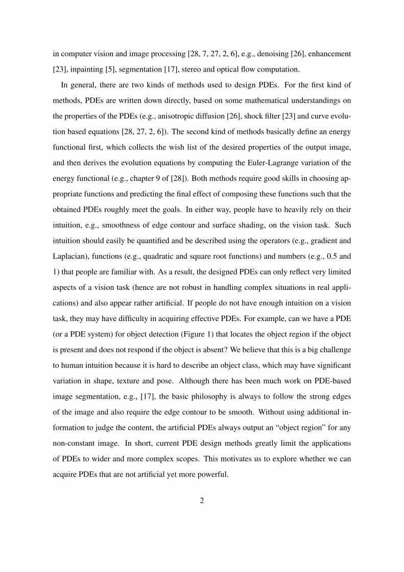
(or a PDE system) for object detection (Figure 1) that locates the object region if the object
is present and does not respond if the object is absent? We believe that this is a big challenge
to human intuition because it is hard to describe an object class, which may have significant
variation in shape, texture and pose. Although there has been much work on PDE-based
image segmentation, e.g., [17], the basic philosophy is always to follow the strong edges
of the image and also require the edge contour to be smooth. Without using additional in-
formation to judge the content, the artificial PDEs always output an “object region” for any
non-constant image. In short, current PDE design methods greatly limit the applications
of PDEs to wider and more complex scopes. This motivates us to explore whether we can
acquire PDEs that are not artificial yet more powerful.
2
Figure 1: What is the PDE (or PDE system) that can detect the object of interest (e.g., planein left image) and does not respond if the object is absent (right image)?
In this paper, we propose a general framework for learning PDEs to accomplish a specific
vision task. The vision task will be exemplified by a number of input-output image pairs,
rather than relying on any form of human intuition. The learning algorithm is based on the
theory of optimal control governed by PDEs [19]. As a preliminary investigation, we assume
that the system consists of two PDEs. One controls the evolution of the output. The other is
for an indicator function that helps collect global information. As the PDEs should be shift
and rotationally invariant, they must be functions of fundamental differential invariants [22].
Currently, we only consider the case that the PDEs are linear combinations of fundamental
differential invariants up to second order. The coupling coefficients are learnt from real data
via the optimal control technique [19]. Our framework can be extended in different ways.
To our best knowledge, the only work of applying optimal control to computer vision and
image processing is by Kimia et al. [15] and Papadakis et al. [25, 24]. However, the work in
[15] is for minimizing known energy functionals for various tasks, including shape evolution,
morphology, optical flow and shape from shading, where the target functions fulfill known
PDEs. The methodology in [25, 24] is similar. Its difference from [15] is that it involves
a control function that appears as the source term of known PDEs. In all existing work
[15, 25, 24], the output functions are those that are desired. While in this paper, our goal
is to determine a PDE system which is unknown at the beginning and the coefficients of the
PDEs are those that are desired.
In principle, our learning-based PDEs form a regressor that learns a high dimensional
mapping function between the input and the output. Many learning/approximation meth-
ods, e.g., neural networks, can also fulfill this purpose. However, learning-based PDEs are
3
fundamentally different from those methods in that those methods learn explicit mapping
functions f : O = f(I), where I is the input and O is the output, while our PDEs learn
implicit mapping functions ϕ: ϕ(I, O) = 0. Given the input I , we have to solve for the
output O. The input dependent weights for the outputs, due to the coupling between the out-
put and the indicator function that evolves from the input, makes our learning-based PDEs
more adaptive to tasks and also require much fewer training samples. For example, we only
used 50-60 training image pairs for all our experiments. Such a number is clearly impossi-
ble for traditional methods, considering the high dimensionality of the images and the high
nonlinearity of the mappings. Moreover, backed by the rich theories on PDEs, it is possible
to better analyze some properties of interest of the learnt PDEs. For example, the theory of
differential invariants plays the key role in suggesting the form of our PDEs.
The rest of this paper is organized as follows. In Section 2, we introduce the related
optimal control theory. In Section 3, we present our basic framework of learning-based
PDEs. In Section 4, we testify to the effectiveness and versatility of our learning-based
PDEs by five vision tasks. In Section 5, we show two possible ways of extending our basic
framework to handle more complicated vision problems. Then we conclude our paper in
Section 6.
2 Optimal Control Governed by Evolutionary PDEs
In this section, we sketch the existing theory of optimal control governed by PDEs that we
will borrow. There are many types of these problems. Due to the scope of our paper, we only
focus on the following distributed optimal control problem:
minimize J(f, u), where u ∈ U controls f via the following PDE: (1)ft = L(⟨u⟩, ⟨f⟩), (x, t) ∈ Q,f = 0, (x, t) ∈ Γ,
f |t=0 = f0, x ∈ Ω,(2)
in which J is a functional, U is the admissible control set and L(·) is a smooth function.
The meaning of the notations can be found in Table 1. To present the basic theory, some
definitions are necessary.
4
Table 1: Notationsx (x, y), spatial variable t temporal variableΩ an open region of R2 ∂Ω boundary of ΩQ Ω× (0, T ) Γ ∂Ω× (0, T )
W Ω, Q, Γ, or (0, T ) (f, g)W
∫W
fgdW
∇f gradient of f Hf Hessian of f℘ ∅, x, y, xx, xy, yy, · · · |p|, p ∈ ℘ ∪ t the length of string p
∂|p|f
∂p, p ∈ ℘ ∪ t f ,
∂f
∂t,∂f
∂x,∂f
∂y,∂2f
∂x2,∂2f
∂x∂y,· · · , when p = ∅, t, x, y, xx, xy, · · ·
fp, p ∈ ℘ ∪ t ∂|p|f
∂p⟨f⟩ fp|p ∈ ℘
P [f ] the action of differential operator P on function f , i.e., if
P = a0 + a10∂
∂x+ a01
∂
∂y+ a20
∂2
∂x2+ a11
∂2
∂x∂y+ · · · , then
P [f ] = a0f + a10∂f
∂x+ a01
∂f
∂y+ a20
∂2f
∂x2+ a11
∂2f
∂x∂y+ · · ·
L⟨f⟩(⟨f⟩, · · · ) the differential operator∑p∈℘
∂L
∂fp
∂|p|
∂passociated to function L(⟨f⟩, · · · )
2.1 Gateaux Derivative of a Functional
Gateaux derivative is an analogy and also an extension of the usual function derivative. Sup-
pose J(f) is a functional that maps a function f on region W to a real number. Its Gateaux
derivative (if it exists) is defined as the function f ∗ on W that satisfies:
(f ∗, δf)W = limε→0
J(f + ε · δf)− J(f)
ε,
for all admissible perturbations δf of f . We may write f ∗ asDJ
Df. For example, if W = Q
and J(f) = 12
∫Ω[f(x, T )− f(x)]2dx, then
J(f + ε · δf)− J(f)
=1
2
∫Ω
[f(x, T ) + ε · δf(x, T )− f(x)]2dΩ− 1
2
∫Ω
[f(x, T )− f(x)]2dΩ
= ε
∫Ω
[f(x, T )− f(x)]δf(x, T )dΩ + o(ε)
= ε
∫Q
[f(x, t)− f(x)]δ(t− T )δf(x, t)dQ+ o(ε),
5
where δ(·) is the Dirac function1. Therefore,
DJ
Df= [f(x, t)− f(x)]δ(t− T ).
2.2 Adjoint Differential Operator
The adjoint operator P ∗ of a linear differential operator P acting on functions on W is one
that satisfies:
(P ∗[f ], g)W = (f, P [g])W ,
for all f and g that are zero on ∂W and are sufficiently smooth2. The adjoint operator can be
found by integration by parts, i.e., using the Green’s formula [8]. For example, the adjoint
where N is the outward normal of Ω and we have used that f and g vanish on ∂Ω.
2.3 Finding the Gateaux Derivative via Adjoint Equation
Problem (1)-(2) can be solved if we can find the Gateaux derivative of J with respect to the
control u: we may find the optimal control u via steepest descent.
Suppose J(f, u) =∫Q
g(⟨u⟩, ⟨f⟩)dQ, where g is a smooth function. Then it can be proved
thatDJ
Du= L∗
⟨u⟩(⟨u⟩, ⟨f⟩)[φ] + g∗⟨u⟩(⟨u⟩, ⟨f⟩)[1], (3)
where L∗⟨u⟩ and g∗⟨u⟩ are the adjoint operators of L⟨u⟩ and g⟨u⟩ (see Table 1 for the notations),
1Please do not confuse with the perturbations of functions.2We are not to introduce the related function spaces in order to make this paper more intuitive.
6
respectively, and the adjoint function φ is the solution to the following PDE:−φt − L∗
⟨f⟩(⟨u⟩, ⟨f⟩)[φ] = g∗⟨f⟩(⟨u⟩, ⟨f⟩)[1], (x, t) ∈ Q,
φ = 0, (x, t) ∈ Γ,φ|t=T = 0, x ∈ Ω,
(4)
which is called the adjoint equation of (2) (note that the adjoint equation evolves backward
in time!). The proof can be found in Appendix 1.
The adjoint operations above make the deduction of the Gateaux derivative non-trivial. As
an equivalence, a more intuitive way is to introduce a Lagrangian function:
J(f, u;φ) = J(f, u) +
∫Q
φ[ft − L(⟨u⟩, ⟨f⟩)]dQ, (5)
where the multiplier φ is exactly the adjoint function. Then one can see that the PDE con-
straint (2) is exactly the first optimality condition:dJdφ
= 0, wheredJdφ
is the partial Gateaux
derivative of J with respect to φ,3 and verify that the adjoint equation is exactly the second
optimality condition:dJdf
= 0. One can also have that
DJ
Du=
dJdu
. (6)
SoDJ
Du= 0 is equivalent to the third optimality condition:
dJdu
= 0.
As a result, we can use the definition of Gateaux derivative to perturb f and u in J and
utilize Green’s formula to pass the derivatives on the perturbations δf and δu to other func-
tions, in order to obtain the adjoint equation andDJ
Du(for an example, see Appendix 3 for
our real computation).
The above theory can be easily extended to systems of PDEs and multiple control function-
s. For more details and a more mathematically rigorous exposition of the above materials,
please refer to [19].
3 Learning-Based PDEs
Now we present our framework of learning PDE systems from training images. As prelimi-
nary work, we assume that our PDE system consists of two PDEs. One is for the evolution3Namely, assuming f , u and φ are independent functions.
7
Table 2: Shift and rotationally invariant fundamental differential invariants up to secondorder.
where Ω is the rectangular region occupied by the input image I , T is the time that the
PDE system finishes the visual information processing and outputs the results, and O0 and
ρ0 are the initial functions of O and ρ, respectively. For computational issues and the ease
of mathematical deduction, I will be padded with zeros of several pixels width around it.
As we can change the unit of time, it is harmless to fix T = 1. LO and Lρ are smooth
functions. a = ai and b = bi are sets of functions defined on Q that are used to control
the evolution of O and ρ, respectively. The forms of LO and Lρ will be discussed below.
8
3.1 Forms of PDEs
The space of all PDEs is infinite dimensional. To find the right one, we start with the proper-
ties that our PDE system should have, in order to narrow down the search space. We notice
that most vision tasks are shift and rotationally invariant, i.e., when the input image is shifted
or rotated, the output image is also shifted or rotated by the same amount. So we require that
our PDE system is shift and rotationally invariant.
According to the differential invariants theory in [22], LO and Lρ must be functions of
the fundamental differential invariants under the groups of translation and rotation. The
fundamental differential invariants are invariant under shift and rotation and other invariants
can be written as their functions. The set of fundamental differential invariants is not unique,
but different sets can express each other. We should choose invariants in the simplest form in
order to ease mathematical deduction and analysis and numerical computation. Fortunately,
for shift and rotational invariance, the fundamental differential invariants can be chosen as
polynomials of the partial derivatives of the function. We list those up to second order in
Table 2.4 As ∇f and Hf change to R∇f and RHfRt, respectively, when the image is
rotated by a matrix R, it is easy to check the rotational invariance of those quantities. In the
sequel, we shall use invi(ρ,O), i = 0, 1, · · · , 16, to refer to them in order. Note that those
invariants are ordered with ρ going before O. We may reorder them with O going before ρ.
In this case, the i-th invariant will be referred to as invi(O, ρ).
On the other hand, for LO and Lρ to be shift invariant, the control functions ai and bi
must be independent of x, i.e., they must be functions of t only. The proof is presented in
Appendix 2.
So the simplest choice of functions LO and Lρ is the linear combination of these differen-
tial invariants, leading to the following forms:
LO(a, ⟨O⟩, ⟨ρ⟩) =16∑j=0
aj(t)invj(ρ,O),
Lρ(b, ⟨ρ⟩, ⟨O⟩) =16∑j=0
bj(t)invj(O, ρ).(8)
4We add the constant function “1” for convenience of the mathematical deductions in the sequel.
9
Note that the visual process may not obey PDEs in such a form. However, we are NOT
to discover what the real process is. Rather, we treat the visual process as a black box and
regard the PDEs as a regressor. We only care whether the final output of our PDE system,
i.e., O(x, 1), can approximate that of the real process. For example, although O1(x, t) =
∥x∥2 sin t and O2(x, t) = (∥x∥2 + (1 − t)∥x∥)(sin t + t(1 − t)∥x∥3) are very different
functions, they initiate from the same function at t = 0 and also settle down at the same
function at time t = 1. So both functions fit our needs and we need not care whether
the system obeys either function. Currently we only limit our attention to second order
PDEs because most of the PDE theories are of second order and most PDEs arising from
engineering are also of second order. It will pose a difficulty in theoretical analysis if higher
order PDEs are considered. Nonetheless, as LO and Lρ in (8) are actually highly nonlinear
and hence the dynamics of (7) can be very complex, they are already complex enough to
approximate many vision tasks in our experiments, as will be shown in Sections 4 and 5. So
we choose to leave the involvement of higher order derivatives to future work.
3.2 Determining the Coefficients by Optimal Control Approach
Given the forms of PDEs shown in (8), we have to determine the coefficient functions aj(t)
and bj(t). We may prepare training samples (Im, Om), where Im is the input image and Om
is the expected output image, m = 1, 2, · · · ,M , and compute the coefficient functions that
minimize the following functional:
J(OmMm=1 , aj
16j=0 , bj
16j=0
)=
1
2
M∑m=1
∫Ω
[Om(x, 1)− Om(x)]2dΩ +
1
2
16∑j=0
λj
∫ 1
0
a2j(t)dt+1
2
16∑j=0
µj
∫ 1
0
b2j(t)dt,(9)
where Om(x, 1) is the output image at time t = 1 computed from (7) when the input image
is Im, and λj and µj are positive weighting parameters. The first term requires that the final
output of our PDE system be close to the ground truth. The second and the third terms are
for regularization so that the optimal control problem is well posed, as there may be multiple
minimizers for the first term. The regularization is important, particularly when the training
10
samples are limited.
Then we may compute the Gateaux derivativeDJ
Dajand
DJ
Dbjof J with respect to aj and
bj using the theory in Section 2. The expressions of the Gateaux derivatives can be found in
Appendix 3. Consequently, the optimal aj and bj can be computed by steepest descent.
3.3 Implementation Details3.3.1 Initial functions of O and ρ
Good initialization increases the approximation accuracy of the learnt PDEs. In our current
implementation, we simply set the initial functions of O and ρ as the input image:
Om(x, 0) = ρm(x, 0) = Im(x), m = 1, 2, · · · ,M.
However, this is not the only choice. If the user has some prior knowledge about the in-
put/output mapping, s/he can choose other initial functions. Some examples of different
choices of initial functions can be found in Section 5.
3.3.2 Initialization of ai and bi
We initialize ai(t) successively in time while fixing bi(t) ≡ 0, i = 0, 1, · · · , 16. Suppose
the time stepsize is ∆t when solving (7) with finite difference. At the first time step, without
any prior information, Om(∆t) is expected to be ∆tOm + (1 −∆t)Im. So ∂Om/∂t|t=∆t is
expected to be Om − Im and we may solve ai(0) such that
s(ai(0)) =1
2
M∑m=1
∫Ω
[16∑j=0
aj(0)invj(ρm(0), Om(0)))− (Om −O0)
]2
dΩ
is minimized, i.e., to minimize the difference between the left and the right hand sides of (7),
where the integration here should be understood as summation. After solving ai(0), we
can have Om(∆t) by solving (7) at t = ∆t. Suppose at the (k + 1)-th step, we have solved
Om(k∆t), then we may expect that Om((k + 1)∆t) = ∆t1−k∆t
Om + 1−(k+1)∆t1−k∆t
Om(k∆t) so
that Om((k + 1)∆t) could move directly towards Om. So ∂Om/∂t|t=(k+1)∆t is expected to
be 11−k∆t
[Om −Om(k∆t)] and ai(k∆t) can be solved in the same manner as ai(0).
11
3.3.3 Choice of Parameters
When solving (7) with finite difference, we use an explicit scheme to solve Om(k∆t) and
ρm(k∆t) successively. However, the explicit scheme is conditionally stable: if the temporal
stepsize is too large, we cannot obtain solutions with controlled error. As we have not investi-
gated this problem thoroughly, we simply borrow the stability condition for two-dimensional
heat equations ft = κ(fxx + fyy):
∆t ≤ 1
4κmin((∆x)2, (∆y)2),
where ∆x and ∆y are the spatial stepsizes. In our problem, ∆x and ∆y are naturally chosen
as 1, and the coefficients of Oxx + Oyy and ρxx + ρyy are a7 and b7, respectively. So the
temporal stepsize should satisfy:
∆t ≤ 1
4max(a7, b7). (10)
If we find that the above condition is violated during optimization at a time step k, we will
break ∆t into smaller temporal stepsizes δt = ∆t/K, such that it satisfies condition (10),
and compute Om(k ·∆t+ i ·δt), i = 1, 2, ..., K, successively until we obtain Om((k+1)∆t).
We have found that this method works for all our experiments.
And there are other parameters to choose. As it does not seem to have a systematic way
to analyze their optimal values, we simply fix their values as: M = 50 ∼ 60, ∆t = 0.05 and
λi = µi = 10−7, i = 0, · · · , 16.
4 Experimental Results
In this section, we present the results on five different computer vision/image processing
tasks: blur, edge detection, denoising, segmentation and object detection. As our goal is to
show that PDEs could be an effective regressor for many vision tasks, NOT to propose better
algorithms for these tasks, we are not going to compare with state-of-the-art algorithms in
every task.
12
Figure 2: Partial results on image blurring. The top row are the input images. The middlerow are the outputs of our learnt PDE. The bottom row are the groundtruth images obtainedby blurring the input image with a Gaussian kernel. One can see that the output of our PDEis visually indistinguishable from the groundtruth.
For each task, we prepare sixty 150×150 images and their ground truth outputs as training
image pairs. After the PDE system is learnt, we apply it to test images. Part of the results
are shown in Figures 2-10, respectively. Note that we do not scale the range of pixel values
of the output to be between 0 and 255. Rather, we clip the values to be between 0 and 255.
Therefore, the reader can compare the strength of response across different images.
For the image blurring task (Figure 2), the output image is expected to be the convolution
of the input image with a Gaussian kernel. It is well known [28] that this corresponds to
evolving with the heat equation. This equation is almost exactly learnt using our method. So
the output is nearly identical to the groundtruth.
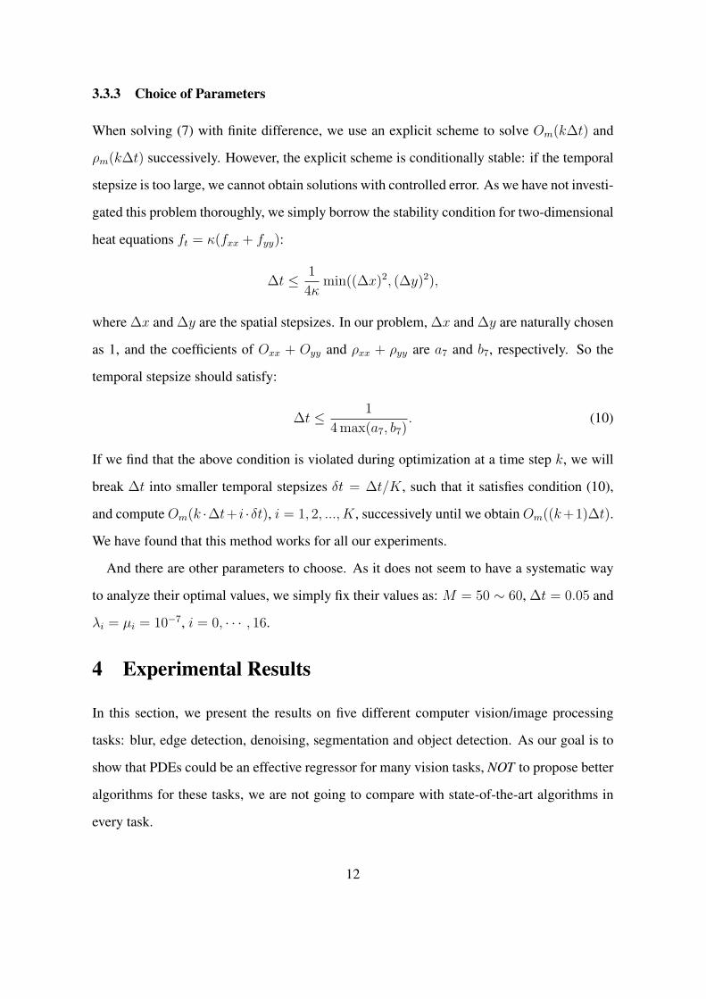
For the image edge detection task (Figure 3), we want our learnt PDE system to approxi-
mate the Canny edge detector. One can see that our PDEs respond strongly at strong edges
and weakly at weak edges. Note that the Canny detector outputs binary edge maps while our
PDEs can only output smooth functions. So it is difficult to approximate the Canny detector
at high precision.
13
Figure 3: Partial results on edge detection. The top row are the input images. The middlerow are the outputs of our learnt PDEs. The bottom row are the edge maps by the Cannydetector. One can see that our PDEs respond strongly at strong edges and weakly at weakedges.
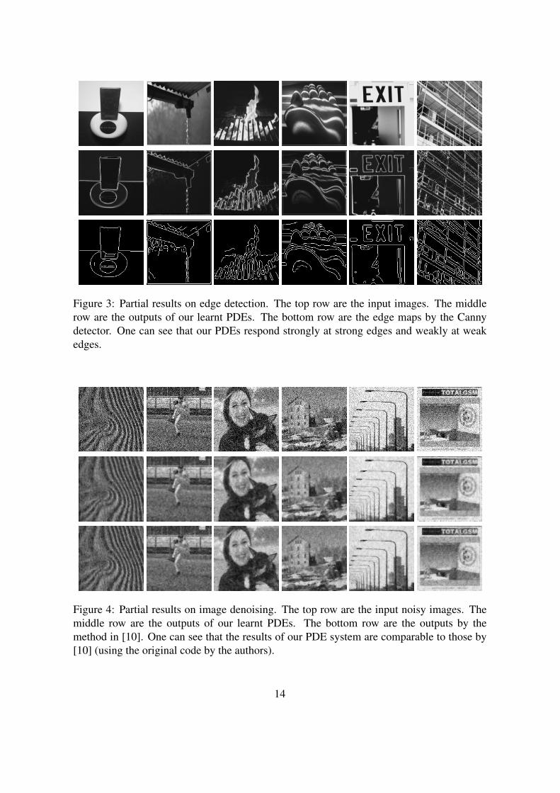
Figure 4: Partial results on image denoising. The top row are the input noisy images. Themiddle row are the outputs of our learnt PDEs. The bottom row are the outputs by themethod in [10]. One can see that the results of our PDE system are comparable to those by[10] (using the original code by the authors).
14
For the image denoising task (Figure 4), we generate input images by adding Gaussian
noise to the original images and use the original images as the ground truth. One can see that
our PDEs suppress most of the noise while preserving the edges well. So we easily obtain
PDEs that produce results comparable with those by [10] (using the original code by the
authors), which was designed with a lot of wits.
While the above three vision problems can be solved by using local information only,
we shall show that our learning-based PDE system is not simply a local regressor. Rather,
it seems that it can automatically find the features of the problem to work with. Such a
global effect may result from the indicator function that is supposed to collect the global
information. We testify this observation by two vision tasks: image segmentation and object
detection.
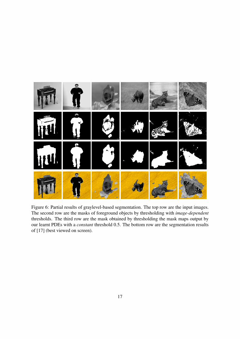
For the image segmentation task, we choose images with the foreground relatively darker
than the background (but the foreground is not completely darker than the background so
that a simple threshold can well separate them, see the second row of Figure 6) and prepare
the manually segmented masks as the outputs of the training images (first row of Figure 5),
where the black regions are the background. The segmentation results are shown in (Fig-
ure 6), where we have thresholded the output mask maps of our learnt PDEs with a constant
threshold 0.5. We see that our learnt PDEs produce fairly good object masks. This may be
because our PDEs correctly identify that graylevel is the key feature. We also test the active
contour method by Li et al. [17] (using the original code by the authors). As it is designed
to follow the strong edges and to prefer smooth object boundaries, its performance is not as
good as ours.
For the object detection task, we require that the PDEs respond strongly inside the object
region while they do not respond (or respond much more weakly) outside the object region.
If the object is absent in the image, the response across the whole image should all be weak
(Figure 1). It should be challenging enough for one to manually design such PDEs. As a
result, we are unaware of any PDE-based method that can accomplish this task. The existing
PDE-based segmentation algorithms always output an “object region” even if the image does
15
(a)
(b)
(c)
(d)
Figure 5: Examples of the training images for image segmentation (top row), butterfly de-tection (second and fourth rows) and plane detection (third and fourth rows). In each groupof images of (a)∼(c), on the left is the input image and on the right is the groundtruth outputmask. In (d), the left images are part of the input images as negative samples for train-ing butterfly and plane detectors, where their groundtruth output masks are all-zero images(right).
16
Figure 6: Partial results of graylevel-based segmentation. The top row are the input images.The second row are the masks of foreground objects by thresholding with image-dependentthresholds. The third row are the mask obtained by thresholding the mask maps output byour learnt PDEs with a constant threshold 0.5. The bottom row are the segmentation resultsof [17] (best viewed on screen).
17
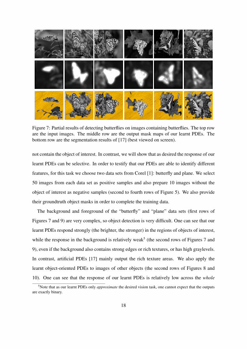
Figure 7: Partial results of detecting butterflies on images containing butterflies. The top roware the input images. The middle row are the output mask maps of our learnt PDEs. Thebottom row are the segmentation results of [17] (best viewed on screen).
not contain the object of interest. In contrast, we will show that as desired the response of our
learnt PDEs can be selective. In order to testify that our PDEs are able to identify different
features, for this task we choose two data sets from Corel [1]: butterfly and plane. We select
50 images from each data set as positive samples and also prepare 10 images without the
object of interest as negative samples (second to fourth rows of Figure 5). We also provide
their groundtruth object masks in order to complete the training data.
The background and foreground of the “butterfly” and “plane” data sets (first rows of
Figures 7 and 9) are very complex, so object detection is very difficult. One can see that our
learnt PDEs respond strongly (the brighter, the stronger) in the regions of objects of interest,
while the response in the background is relatively weak5 (the second rows of Figures 7 and
9), even if the background also contains strong edges or rich textures, or has high graylevels.
In contrast, artificial PDEs [17] mainly output the rich texture areas. We also apply the
learnt object-oriented PDEs to images of other objects (the second rows of Figures 8 and
10). One can see that the response of our learnt PDEs is relatively low across the whole
5Note that as our learnt PDEs only approximate the desired vision task, one cannot expect that the outputsare exactly binary.
18
Figure 8: Partial results of detecting butterflies on images without butterflies. The top roware the input images. The middle row are the output mask maps of our learnt PDEs. Thebottom row are the segmentation results of [17] (best viewed on screen). Please be remindedthat the responses may appear stronger than they really are, due to the contrast with the darkbackground.
Figure 9: Partial results of detecting planes on images containing planes. The top row arethe input images. The middle row are the output mask maps of our learnt PDEs. The bottomrow are the segmentation results of [17] (best viewed on screen).
19
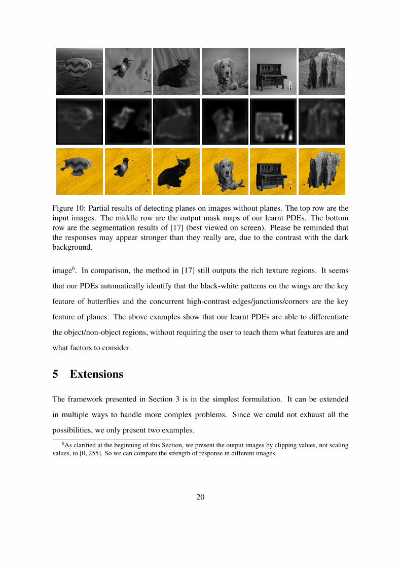
Figure 10: Partial results of detecting planes on images without planes. The top row are theinput images. The middle row are the output mask maps of our learnt PDEs. The bottomrow are the segmentation results of [17] (best viewed on screen). Please be reminded thatthe responses may appear stronger than they really are, due to the contrast with the darkbackground.
image6. In comparison, the method in [17] still outputs the rich texture regions. It seems
that our PDEs automatically identify that the black-white patterns on the wings are the key
feature of butterflies and the concurrent high-contrast edges/junctions/corners are the key
feature of planes. The above examples show that our learnt PDEs are able to differentiate
the object/non-object regions, without requiring the user to teach them what features are and
what factors to consider.
5 Extensions
The framework presented in Section 3 is in the simplest formulation. It can be extended
in multiple ways to handle more complex problems. Since we could not exhaust all the
possibilities, we only present two examples.
6As clarified at the beginning of this Section, we present the output images by clipping values, not scalingvalues, to [0, 255]. So we can compare the strength of response in different images.
20
5.1 Handling Vectored-Valued Images5.1.1 Theory
For color images, the design of PDEs becomes much more intricate because the correlation
among different channels should be carefully handled so that spurious colors do not appear.
Without sufficient intuitions on the correlation among different channels of images, people
either consider a color image as a set of three images and apply PDEs independently [5], or
use LUV color space instead, or from some geometric considerations [29]. For some vision
problems such as denoising and inpainting, the above mentioned methods may be effective.
However, for more complex problems, such as Color2Gray [11], i.e., keeping the contrast
among nearby regions when converting color images to grayscale ones, and demosaicking,
i.e., inferring the missing colors from Bayer raw data [18], these methods may be incapable
as human intuition may fail to apply. Consequently, we are also unaware of any PDE related
work for these two problems.
Based on the theory presented in Section 3, which is for grayscale images, having PDEs
for some color image processing problems becomes trivial, because we can easily extend the
framework in Section 3 for learning a system of PDEs for vector-valued images. With the ex-
tended framework, the correlation among different channels of images can be automatically
(but implicitly) modelled. The modifications on the framework in Section 3 include:
1. A single output channel O now becomes multiple channels: Ok, k = 1, 2, 3.
2. There are more shift and rotationally invariant fundamental differential invariants. The
set of such invariants up to second order is as follows:
1, fr, (∇fr)
t∇fs, (∇fr)tHfm∇fs, tr(Hfr), tr(HfrHfs)
where fr, fs and fm could be the indicator function ρ or either channel of the output
image. Now there are 69 elements in the set.
3. The initial function for the indicator function is the luminance of the input image.
21
Figure 11: Comparison of the results of Photoshop Grayscale (second row), our PDEs (thirdrow) and Color2Gray [11] (fourth row). The first row are the original color images. Theseimages are best viewed on screen.
22
4. The objective functional is the sum of J’s in (9) for every channel (with 16 changed to
68).
Note that for vectored-valued images with more than three channels, we may simply increase
the number of channels. It is also possible to use other color spaces. However, we deliber-
ately stick to RGB color space in order to illustrate the power of our framework. We use the
luminance of the input image as the initial function of the indicator function because lumi-
nance is the most informative component of a color image, in which most of the important
structural information, such as edges, corners and junctions, is well kept.
5.1.2 Experiment
We test our extended framework on the Color2Gray problem [11]. Contrast among nearby
regions is often lost when color images are converted to grayscale by naively computing their
luminance (e.g., using using Adobe Photoshop Grayscale mode). Gooch et al. [11] proposed
an algorithm to keep the contrast by attempting to preserve the salient features of the color
image. Although the results are very impressive, the algorithm is very slow: O(S4) for an
S×S square image. To learn the Color2Gray mapping, we choose 50 color images from the
Corel database and generate their Color2Gray results using the code provided by [11]. These
50 input/output image pairs are the training examples of our learning-based PDEs. We test
the learnt PDEs on images in [11] and their websites7. All training and testing images are
resized to 150 × 150. Some results are shown in Figure 11.8 One can see (best viewed on
screen) that our PDEs produce comparable visual effects to theirs. Note that the complexity
of mapping with our PDEs is only O(S2): two orders faster than the original algorithm.
5.2 Multi-Layer PDE Systems5.2.1 Theory
Although we have shown that our PDE system is a good regressor for many vision tasks,
it may not be able to approximate all vision mappings at a desired accuracy. To improve7http://www.cs.northwestern.edu/∼ago820/color2gray/8Due to resizing, the results of Color2Gray in Figure 11 are slightly different from those in [11].
23
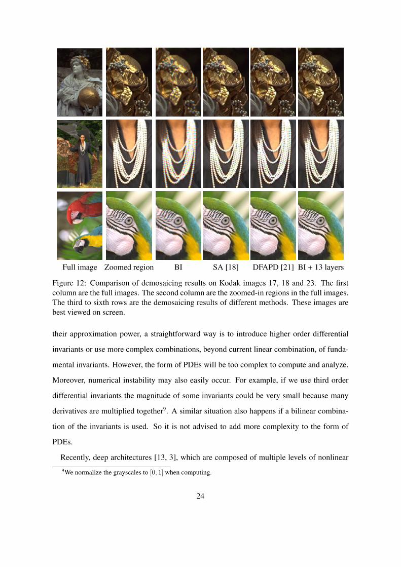
Full image Zoomed region BI SA [18] DFAPD [21] BI + 13 layers
Figure 12: Comparison of demosaicing results on Kodak images 17, 18 and 23. The firstcolumn are the full images. The second column are the zoomed-in regions in the full images.The third to sixth rows are the demosaicing results of different methods. These images arebest viewed on screen.
their approximation power, a straightforward way is to introduce higher order differential
invariants or use more complex combinations, beyond current linear combination, of funda-
mental invariants. However, the form of PDEs will be too complex to compute and analyze.
Moreover, numerical instability may also easily occur. For example, if we use third order
differential invariants the magnitude of some invariants could be very small because many
derivatives are multiplied together9. A similar situation also happens if a bilinear combina-
tion of the invariants is used. So it is not advised to add more complexity to the form of
PDEs.
Recently, deep architectures [13, 3], which are composed of multiple levels of nonlinear
9We normalize the grayscales to [0, 1] when computing.
24
operations, are proposed for learning highly varying functions in vision and other artificial
intelligence tasks [4]. Inspired by their work, we introduce a multi-layer PDE system. The
forms of PDEs of each layer are the same, i.e., linear combination of invariants up to second
order. The only difference is in the values of the control parameters and the initial values
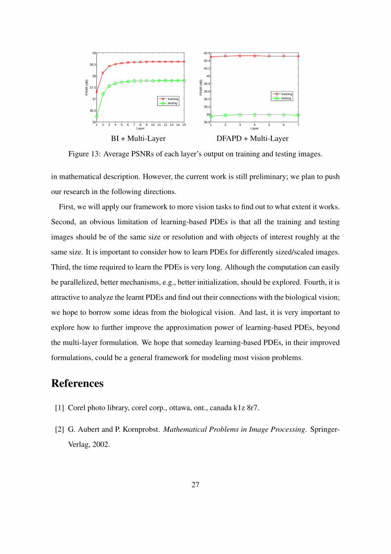
of all the functions, including the indicator function. The multi-layer structure is learnt by
adopting a greedy strategy. After the first layer is determined, we use the output of the
previous layer as the input of the next layer. The expected output of the next layer is still
the ground truth image. The optimal control parameters for the next layer are determined as
usual. As the input of the next layer is expected to be closer to the ground truth image than
the input of the previous layer, the approximation accuracy can be successively improved.
If there is prior information, such a procedure could be slightly modified. For example, for
image demosaicing, we know that the Bayer raw data should be kept in the output full-color
image. So we should replace the corresponding part of the output images with the Bayer
raw data before feeding them to the next layer. The number of layers is determined by the
training process automatically, e.g., the layer construction stops when a new layer does not
result in output images with smaller error from the ground truth images.
5.2.2 Experiment
We test this framework on image demosaicking. Commodity digital cameras use color fil-
ter arrays (CFAs) to capture raw data, which have only one channel value at each pixel.
The missing channel values for each pixel have to be inferred in order to recover full-color
images. This technique is called demosaicing. The most commonly used CFAs are Bayer
pattern [12, 18, 21]. Demosaicing is very intricate as many artifacts, such as blur, spuri-
ous color and zipper, may easily occur, and numerous demosaicing algorithms have been
proposed (e.g., [12, 18, 21]). We show that with learning-based PDEs, demosaicing also
becomes easy.
We used the Kodak image database10 for the experiment. Images 1-12 are used for training
10The 24 images are available at http://www.site.uottawa.ca/∼edubois/demosaicking
25
Table 3: Comparison on PSNRs of different demosaicing algorithms. “BI + 1 layer” de-notes the results of single-layer PDEs using bilinearly interpolated color images as the initialfunctions. Other abbreviations carry the similar meaning.
BI AP [12] SA [18] DFAPD [21]Avg. PSNR (dB) 29.62± 2.91 37.83± 2.57 38.34± 2.56 38.44± 3.04