1

Learning serial constraint-based grammars Robert Staubs and Joe Pater, University of Massachusetts Amherst

1 Introduction

In this paper we describe a method for learning grammars in the general framework of Harmonic Serialism (see McCarthy this volume for references and an introduction). We have two main goals. The first is to address the hidden structure problem that serial derivations introduce. The second is to address the problem of learning variation, which has yet to be confronted in this framework (see also Staubs et al. 2010 and Tessier and Jesney 2014 on the learning of Harmonic Serialism). In the remainder of this section, we illustrate the grammar model, and our approach to the learning of hidden structure, with a simple example of stress-epenthesis interaction. Our main contribution comes in the next section, where we introduce a method for calculating probabilities over the unbounded non-monotonic derivations that are characteristic of a stochastic serial theory. The third and last section consists of an application to data from French ‘schwa’ deletion that display variation.

In Harmonic Serialism, the path from the grammar’s initial input to its final output is a series of derivational steps. In each step, a set of operations first applies to create a candidate set of outputs, from which one is chosen by a set of constraints. This output becomes the input for the next step of the derivation. The derivation terminates, or converges, when the chosen output is identical to the input of that step. From the perspective of learning, these derivations are an instance of what Tesar and Smolensky (2000) call ‘hidden structure’. Hidden structure refers to properties of the learning data that are not supplied to the learner, but must instead be inferred as part of the learning process. Our approach to learning this case of hidden structure is a generalization of Eisenstat’s (2009) method for learning phonological Underlying Representations (URs). We will explain and illustrate Eisenstat’s proposal as we discuss our toy stress-epenthesis case, since it also includes a UR learning problem.

The words in our mini-language are [tikát] and [píkat], stressed on the second and first syllable respectively. These surface forms can be produced by the derivations shown in (1). This is the standard rule-based analysis of opaque stress-epenthesis interaction (Brame 1974). As Elfner (this volume) shows, Harmonic Serialism can also produce derivations that follow these steps.

2

(1) /tkat/ /pikat/ UR

tkát píkat Stress tikát – Epenthesis [tikát] [píkat] SR

The data given to the learner are the overt forms [tikát] and [píkat]. We do not include any hidden structure in the Surface Representations (SRs), such as metrical structure, so the overt forms and SRs are equivalent.

One type of hidden structure that the learner must discover is the UR for each SR. Here we restrict the search space to /tkat/ and /tikat/, and /pkat/ and /pikat/. In Eisenstat’s (2009) model, the probabilities of the overt forms are the summed probabilities of the UR-SR mappings corresponding to each. Thus for our example the probabilities of [tikát] and [píkat] are calculated as in (2).

(2) Probabilities of overt forms as summed probabilities of UR-SR mappings

p ([tikát]) = p (/tkat/ →  [tikát]) + p (/tikat/ →  [tikát])

p ([píkat]) = p (/pkat/ →  [píkat]) + p (/pikat/ →  [píkat])

The learning objective is to maximize the probability or likelihood that the grammar assigns to the observed overt forms. We will discuss how this is done shortly.

In the serial setting, the steps between the underlying form and the surface form are further instances of hidden structure. Here we assume that each step of the derivation adds the epenthetic vowel [i], or a stress to a syllable of a word that lacks it. When the derivation starts with a UR that lacks [i] and stress, like /tkat/, there are thus two paths that lead to an SR like [tikát] with stress on the final syllable, with either epenthesis or stress placement applying first. The probability of an overt form is now the summed probability of the derivations that lead to it, as shown in (3).

(3) Probabilities of overt forms as summed probabilities of derivations

p ([tikát]) = p (/tkat/ →  tikat  → [tikát]) + p (/tkat/ →  tkát  →  [tikát]) + p (/tikat/ →  [tikát])

p ([píkat]) = p (/pkat/ →  pikat    → [píkat]) + p (/pikat/ →  [píkat])

The probability of each of the derivations is the product of the probabilities of each of its steps. The probability of each of the steps is the probability that the grammar grants to that outcome relative to all other possible outcomes of that step, that is, relative to all of the other members of the current candidate set.

3

Like Eisenstat (2009) we use Goldwater and Johnson’s (2003) Maximum Entropy Grammar

(MaxEnt) to define the probability distribution over a candidate set. Our learning proposal is in principle compatible with other stochastic variants of Optimality Theory (OT) and Harmonic Grammar (HG) (see Coetzee and Pater 2011 for an overview and Kimper 2011a on a serial implementation), but MaxEnt has a conveniently direct definition of probability. MaxEnt is a probabilistic version of HG in that it computes the Harmony of each candidate as the weighted sum of constraint violations (see Pater this volume for an introduction to and overview of HG, and Boersma and Pater this volume on Noisy HG, another stochastic implementation). In MaxEnt, the probability of a candidate is proportional to the exponential of its Harmony. MaxEnt in a serial framework is thus a probabilistic version of serial HG; for other work in serial HG see Elfner (this volume), Kimper (2011b), Mullin (2011) and Pater (2012, this volume).

For this example, which includes UR learning, we also follow Eisenstat (2009) and Pater, et al. (2012) in using constraints on URs, first introduced to OT by Zuraw (2000) and Boersma (2001), and first applied to the learning of underlying forms by Apoussidou (2007). These constraints demand particular mappings from meaning (or morpho-syntactic features) to phonological URs (our formalism differs somewhat from earlier proposals; see also Pater et al. 2012). Here we have the set of four UR constraints in (4a), which assign violations as in (4b). We give [píkat] the meaning ‘paper’, and [tikát] the meaning ‘table’.

(4) UR constraints a. ‘paper’ →  /pkat/ b. ‘paper’ →  /pikat/  c.  ‘table’  →  /tkat/  d.  ‘table’  →  /tikat/  b. Assign  a  penalty  of  –1  if  meaning  ‘X’  does  not  map  to  UR  /Y/

Our derivations start with an input meaning, and a candidate set of the two URs that satisfy each of the two constraints for each meaning. At this initial step of the derivation, the only constraints that apply are the UR constraints, and these constraints do not apply to any of the further steps of the derivation. The assumption that the phonological constraints do not apply at the step of UR insertion is not crucial; we make it only to produce derivations that look more like standard rule-based ones (see Wolf 2008 for relevant discussion).

The tableau in (5) illustrates the first step of a derivation from ‘table’. The weights of the constraints are shown underneath the constraint names; these are the weights that our learner found in a simulation with overt [tikát] and [píkat] (paired with their meanings). The Harmony scores for each of the candidate URs is shown to the right of the row. Beside each of the candidate URs is its probability under the MaxEnt definition given above, rounded to three

4

decimal points (‘1’ = 1.000). With these weights, /tikat/ is vanishingly improbable as the first step.

(5) First step of a derivation from ‘table’

‘table’ ‘table’  →  /tkat/  

7.94 ‘table’  →  /tikat/  

0

a. 1 /tkat/ –1 0

b. 0 /tikat/ –1 –7.94

We will follow the derivational path for the highly likely /tkat/.

The candidate sets in subsequent steps consist of the unchanged input, as well as all results of applying one of two operations. Stress placement adds stress to any syllable, if a word does not already have a stress. Epenthesis adds the vowel [i] between any two adjacent consonants. The candidate sets are evaluated by the constraints STRESS-L and STRESS-R, which demand stress on the leftmost and rightmost syllable respectively, and assign a violation if that syllable is not stressed, as well as by *CLUSTER, which penalizes adjacent consonants.

The tableau for the second step of the derivation shows the activity of these operations and constraints. The unchanged (6a.) violates all three constraints, and thus has very low probability. Adding a vowel, as in (6b.), resolves the *CLUSTER violation, but still incurs violations of the stress constraints. Since [tkát] is monosyllabic, it satisfies both stress constraints, at the cost of retaining the *CLUSTER violation. In (6) the sum of the weights of the stress constraints is greater than the weight of the *CLUSTER constraint, so [tkát] has higher probability than [tikat].1 This shows how the constraints can affect the order of operations: with these weights, stress is extremely likely to precede epenthesis.

(6) Second step of a derivation from ‘table’

/tkat/ STRESS-­‐R  

12.01 STRESS-­‐L  

18.57  *CLUSTER  

24.42  

a. 0 tkat –1 –1 –1 –55.01

b. 0.002 tikat –1 –1 –30.58

c. 0.998 tkát –1 –24.43

We again follow the path resulting from the most probable output. In the next step, the only available operation is epenthesis, since we are assuming stress placement only applies to

5

unstressed words. Adding the vowel as in (7b.) adds a violation of STRESS-L relative to the unchanged form in (7a.), because the leftmost syllable is now unstressed. The unchanged (7a.), on the other hand, retains the violation of *CLUSTER. With *CLUSTER having a higher weight than STRESS-L, [tikát] gets higher probability than [tkát].

(7) Third step of a derivation from ‘table’

tkát STRESS-­‐R  

12.01 STRESS-­‐L  

18.57  *CLUSTER  

24.42  

a. 0.001 tkát –1 –24.42

b. 0.999 tikát –1 –18.57

With [tikát] as an input, there are no further operations that can apply, so [tikát] will be the sole output candidate, and the derivation will thus converge.

Given ‘table’ as the initial input, the probability of this derivation is nearly 1, so the observed [tikát] with second syllable stress has probability approaching its maximum. These weights also give observed [píkat] with initial stress probability approaching 1. The difference between them comes from the difference in the weights of their respective UR constraints. As shown in (8), ‘paper’ is extremely likely to map in the first step to bisyllabic /pikat/.    

(8) First step of a derivation from ‘paper’

‘paper’ ‘paper’  →  /pkat/  

0 ‘paper’  →  /pikat/  

7.94

a. 0 /pkat/ –1 –7.94

b. 1 /pikat/ –1 0

The next step in the derivation, from /pikat/, is shown in (9).

6

(9) Second step of a derivation from ‘paper’

/pikat/ STRESS-­‐R  

12.01 STRESS-­‐L  

18.57  *CLUSTER  

24.42  

a. 0.001 pikát –1 –12.01

b. 0.999 píkat –1 –18.57

c. 0 pikat –1 –1 –30.58

The most probable outcome is the observed [píkat] because STRESS-L has a greater weight than STRESS-R. The next step of the derivation converges on this form, since neither operation can apply.

We have now explained and illustrated how the grammar produces probabilities over the overt forms as the sum of probabilities of the derivations leading to them, with the probabilities of the derivations themselves arising as joint probabilities of their steps. We are therefore now ready to explain how the learner finds the constraint weights that yield the probabilities over the candidate sets. As we mentioned above, the learning objective is to maximize the likelihood of the observed forms. In a weighted constraint approach, the variables that the learner manipulates are the constraint weights. Set up in this way, this optimization problem can be solved by a range of algorithms. The particular optimization algorithm we used was the L-BFGS-B method (Byrd et al. 1995) as implemented in R (R Development Core Team 2010). L-BFGS-B is a quasi-Newton method implementing box constraints on solutions. We use these box constraints to set a zero minimum for constraint weights. The only remaining issue is that the solution space is unbounded above, because with finite weights the probability that the grammar assigns to the observed forms can only approach 1. To resolve this, we take the standard approach of adding to the objective function a regularization term that penalizes the constraint weights in proportion to their distance from zero. The weights shown above were found with a Gaussian (or L2) prior with variance 100,000, which is sufficiently weak that it does little more than stop the weights from going to infinity.

In the general case, the calculation of the probabilities over overt forms that the grammar generates is more complex than in our toy example. The simplicity of the calculation above was due to the monotonic nature of the derivations: structure was only added, and never taken away or changed. The complexity of the general case can be appreciated by considering the result of adding an operation that deletes the vowel [i]. The set of derivations leading to [tikát] is now infinite – a few paths are illustrated in (10).

7

(10) A sample of an infinite set of derivations with the same result

a. /tkat/ →  tikat  → tikát  → [tikát] b. /tkat/ →  tikat  → tikát  →  tkát  →  tikát → [tikát] c. /tkat/ →  tikat  → tikát  →  tkát  →  tikát → tkát  → tikát → [tikát]

The path in (10a.) is the one that our grammar produced with probability approaching 1. The path in (10b.) results from deleting [i] after placing stress, and reinserting it, and (10c.) iterates this loop. Deletion is preferred by STRESS-L, and insertion by *CLUSTER, so even if we remove harmonically bounded candidates (see section 2), there is always some probability of choosing the result of these operations rather than the unchanged form, thus postponing convergence. The length of the derivations is therefore unbounded, and the set of derivations producing the same result is infinite. As Kimper (2011a: 458) points out, in a stochastic serial theory the probability of non-convergence in such cases becomes arbitrarily close to zero as derivation length increases. The issue for our learning model, which we address in the next section, is how to calculate probabilities over infinite sets of paths like those in (10) that lead from a given initial input to the same final output.

2 Computing probabilities over unbounded derivations

2.1. Unbounded derivations

To discuss our approach to unbounded derivations, we will use a schematic case involving obstruent voicing. The input /bada/ has two voiced obstruents. Figure 1 depicts the possible derivations starting from this input as a directed graph. Here the operations assumed in GEN are simply VOICE and DEVOICE — that is, the voicing of an obstruent can be changed in either direction. The one exception is that [pada] does not map to [bada], because [pada] harmonically bounds [bada] with our constraint set – we return to this point in section 2.2.

Figure 1. Graph of space of derivations for voicing example

8

From the input /bada/, an output [pata] is reachable in a number of ways, as shown in the sample of derivational paths in (11).

(11) Derivational paths from /bada/ to [pata] /bada/ → pada → pata → [pata] /bada/ → bata → pata → [pata] /bada/ → bata → bada → bata → pata → [pata] /bada/ → bata → pata → pada → pata → [pata] …

A given derivation may meander through the graph in any way that obeys the directions of its arcs. It is only when the derivation ‘loops’ back on a single particular node that it enters a convergence state and the derivation as a whole converges. Thus, in general, the length of derivations is unbounded, and the number of them producing a particular output for a given input is infinite.

If the number of derivations producing an input/output mapping is infinite, we must incorporate this knowledge into our computation of derivational probabilities. This incorporation will in effect sum over the infinite number of possible derivations, yielding a probability distribution over convergence states. We return to the details of this computation after first discussing the construction of graphs like Figure 1.

2.2. From operations to graphs

In order to explicitly calculate derivational probabilities, we will require an explicit representation of the possible steps of a serial derivation in the given domain. In particular, given a set of operations GEN and a set of constraints CON we must be able to construct a graph like Figure 1 depicting the possible transitions between two steps.

Such graphs allow the finite representation of an infinite number of derivations. This finiteness is crucial for the approach adopted here. Finiteness follows immediately from non-probabilistic serial constraint-based theories: any particular Harmonic Serialist derivation has only a finite potential for improvement under a given ranking of the constraints in CON and must always improve harmony, step by step. Taken together, these facts imply that all Harmonic Serialist derivations are of bounded length (McCarthy, 2008:274). Thus the possible steps included in a derivational graph should include at least all steps (eventually) derivable from the input(s) through operations in GEN whose results are not harmonically bounded in their candidate sets according to the constraint set CON (where a harmonically bounded

9

candidate has a proper superset of violation marks of another member of the same candidate set). This criterion yields the set of derivations fulfilling the criterion of (potential) harmonic improvement.

With a non-probabilistic model, the set of all steps to non-harmonically bounded candidates provides the full space of possible derivations. This is true also of any probabilistic framework that guarantees that harmonically bounded candidates do not receive any probability mass. Of the OT and HG theories of stochastic grammar surveyed in Coetzee and Pater (2011), only MaxEnt grants probability to harmonically bounded forms (see Jäger and Rosenbach 2006, Jesney 2011 on this aspect of MaxEnt). Since we adopt MaxEnt to define probabilities over candidate sets, we must instead impose an additional delimiting heuristic on the space of derivations in order to avoid creating infinite graphs. For example, a finite graph is guaranteed to exist if only non-harmonically bounded candidates are permitted, as in the graph in Figure 1.2

With the criteria described here we can create graphs describing the derivational spaces relevant to arbitrary sets GEN and CON. With these mechanisms in place we can proceed to the calculation of probabilities over the final outputs of the grammar.

2.3. Derivations as Markov chains

Given a particular weighting of constraints, the space of derivations does not simply look like Figure 1. Arcs are not merely present or absent; instead, arcs are annotated by their various probabilities of occurrence. Figure 1 can thus be written as in Figure 2.

Figure 2. Markov chain for voicing example

Here the probabilities are those given by a Maximum Entropy model with the following constraints: IDENT(voice) (‘do not change voicing,’ w = 1.5), *VOICE (‘do not have voicing in the output,’ w = 3.0), and *VtV (‘do not have voiceless obstruents between vowels in the output,’ w = 2.0).

10

Written in this form, the derivational space is a particular type of probabilistic graph known

as a Markov chain. Derivational Markov chains have a particularly useful property: they are absorbing. From any given step of a derivational chain, there must be at least one convergence state reachable from that step. Once a derivation enters one of these convergence states, the derivation has ‘converged’ and may not leave that state. In the terminology of Markov chains, these states are absorbing states. States that are not absorbing are called transient. A Markov chain of this sort permits us to perform some helpful manipulations for calculating derivational probabilities.

To proceed we restate the information contained within the graph itself in the form of a matrix P. Each row (and column) of the matrix corresponds to a particular state (i.e. derivational step). The values in the matrix are transitional probabilities. Thus the value in a particular row and column is the probability of moving between the state represented by that row and the state represented by that column.

Figure 3. Transition matrix for voicing case. Forms in square brackets represent convergent states.

We can arrange this matrix so that transient states are listed first by both columns and rows. We can then partition the transition matrix of an absorbing Markov chain in the following way. The upper-left portion (corresponding to transient-transient mappings) we call Q. The upper-right portion (transient-absorbing mappings) we call R. As the derivation never leaves absorbing states, the lower-left (absorbing-transient) is a zero matrix 0. Finally, as absorbing states must self-loop, the lower-right (absorbing-absorbing) is an identity matrix 1 with the same number of rows and columns as there are absorbing states.

11

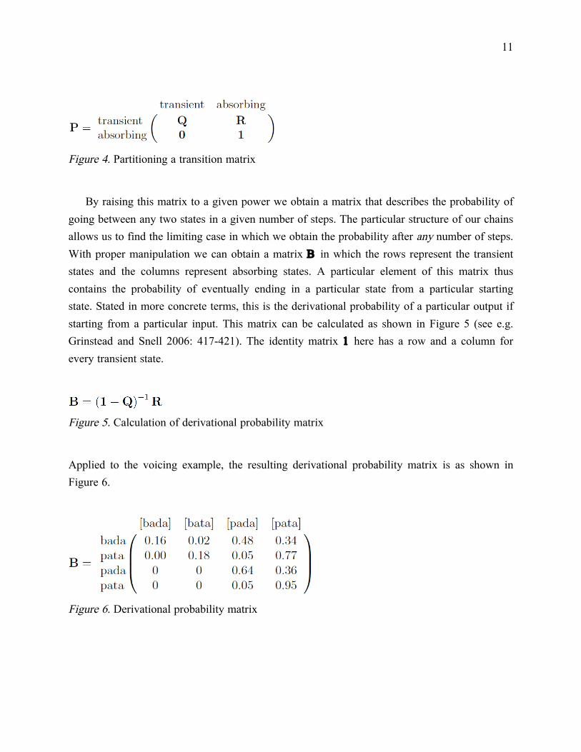
Figure 4. Partitioning a transition matrix

By raising this matrix to a given power we obtain a matrix that describes the probability of going between any two states in a given number of steps. The particular structure of our chains allows us to find the limiting case in which we obtain the probability after any number of steps. With proper manipulation we can obtain a matrix B in which the rows represent the transient states and the columns represent absorbing states. A particular element of this matrix thus contains the probability of eventually ending in a particular state from a particular starting state. Stated in more concrete terms, this is the derivational probability of a particular output if starting from a particular input. This matrix can be calculated as shown in Figure 5 (see e.g. Grinstead and Snell 2006: 417-421). The identity matrix 1 here has a row and a column for every transient state.

Figure 5. Calculation of derivational probability matrix

Applied to the voicing example, the resulting derivational probability matrix is as shown in Figure 6.

Figure 6. Derivational probability matrix

12

The probability of going from an initial input /bada/ to any of the possible output forms is given in the first row of B. Note that this result differs from the individual step probabilities; we will return to this point in the next section.

2.4. Error minimization

In the preceding subsections we detailed a way of calculating the probabilities over final outputs given an initial input, as well as a particular GEN, CON, and constraint weighting. We must also consider how weights may be learned given an observed distribution over mappings from initial inputs to final outputs. In section 1 we stated the learning objective as maximizing the probability of the observed final outputs, which each had probability 1. Here we state the objective as error minimization, which is a more general formulation that is also suitable for real numbered probabilities over final outputs.

A standard measure of model error is Kullback-Leibler (KL) divergence between the observed distribution p and the fitted distribution q (Kullback and Leibler 1951). The KL divergence between two distributions is the average log difference between them, with the average taken in terms of p. It is minimized (at zero) if and only if p and q are equal. Thus by picking weights w to minimize the KL divergence between the two distributions, we are choosing weights which best match the observed distribution.

Figure 7. KL minimization

In the present context, the observed and fitted distributions are probability distributions over the possible final outputs for each of a set of initial inputs; to get single distributions for optimization, we average over all inputs in calculating p and q, giving equal weight to the distribution for each input. The observed distributions for each input are given to the learner. Given the construction of the probability matrix B in the preceding section, we may easily calculate the output distributions for each input, and hence values of q. By numerically minimizing KL, then, we are finding weights that come as close as possible to producing the observed probability distributions.

13

3 An application to variation

In the previous section, an abstract example was used to illustrate the calculation of probabilities over unbounded derivations. In that example, a pair of obstruents in a word like /bada/ changed their voicing back and forth from voiced to voiceless, travelling through the representational space of {[bada], [bata], [pada], [pata]}. Here we apply the learning model to a case of variation in natural language that can be characterized in a similar way. French ‘schwa’ is usually an orthographic ‘e’ and a phonetic back rounded vowel [œ]: the term schwa is used to refer to those instances of this vowel that alternate with zero. Given a phrase like je me prépare, where je and me both contain schwa, we will consider a representational space consisting of the four possibilities resulting from each vowel being pronounced or not. This space is illustrated in (12), using the French orthographic convention of notating a deleted schwa with an apostrophe.

(12) Representational space for je me prépare ‘I prepare myself’

a. Je me prépare

b. J’ me prépare

c. Je m’ prépare

d. J’ m’ prépare

Our operations are schwa insertion and deletion, which can take either (12a.) or (12d.) back and forth from either (12b.) or (12c.). As in the example in section 1, vowel insertion only inserts a vowel between two consonants, thus keeping the representational space finite.

We model some impressionistic data on the relative probability of the two pronunciations in (12b.) and (12c.) from Delattre (1949b: 46), who notes when a schwa is deleted, it is usually the second one, as in (12c.), but that the first schwa is also sometimes lost, as in (12b.). He estimates the occurrence of (12b.) as ‘…disons – moins d’une fois sur dix’ (‘let’s say less than once in ten’). We also include the contrastive case of je te répondrais, which Delattre states is usually pronounced with initial deletion as j’te répondrais, and sometimes as je t’ répondrais, ‘peut-être une fois sur vingt’ (‘maybe once in twenty’).

We use four constraints to derive this pattern. Delattre (1949ab) and Côté (2000) attribute the relative ill-formedness of je t’ répondrais to stops being difficult to produce and/or perceive without a following vowel. For the forms we are considering, in which [t] is the only stop, we use a constraint *t’ that penalizes [t] without a following schwa. Along the same lines, we might attribute the general preference for retention of the initial schwa to the fact that this

14

allows both of the consonants to be adjacent to a vowel. For our data, it is sufficient to have a constraint *j’ that penalizes [ʒ] without a following schwa. As the constraint to motivate deletion we use simple *SCHWA, which penalizes each pronounced schwa. Finally, we also include a constraint that penalizes deletion of both schwas, as in (12d.). Following Grammont (1894), we use a constraint against a sequence of three consonants, *CCC. In all of this we simplify greatly relative to the complexity of actual French; see Eychenne (2006) for a recent overview of the generative literature.

We provided our learner with the distributions over the output patterns shown in the ‘Obs.’ (for Observed) column of (13). The relative probabilities of forms in rows (13b.) vs. (13c.) correspond to Delattre’s estimates. J’ me prépare is ‘less than one in ten’ with respect to Je m’ prépare and Je t’ répondrais is ‘one in twenty’ with respect to J’ te répondrais. French schwa deletion is generally described as optional, so the forms in row (13a.) must have some probability, but Delattre (1949ab) does not give any information about the likelihood of these types of pronunciation. We used values that our grammar model could represent.3 In particular, because the low probability of je t’ répondrais requires a relatively high weighted *t’ constraint, je te répondrais must get higher probability than je me prépare.

(13) Distributions in learning data (Obs.), and produced by the grammar (Fit.) Obs. Fit. Obs. Fit. a. Je me prépare 0.13 0.125 Je te répondrais 0.6 0.605 b. J’ me prépare 0.07 0.075 J’ te répondrais 0.38 0.374 c. Je m’ prépare 0.8 0.8 Je t’ répondrais 0.02 0.02 d. J’ m’ prépare 0 0 J’ t’ répondrais 0 0

In this simulation, we abstracted from UR learning by assuming schwa-ful je, me and te (/ʒœ/, /mœ/, /tœ/) as underlying representations. The constraint weights were found using the same parameters as in section 1, that is, L-BFGS-B with regularization variance 100,000 and starting weights of zero. The ‘Fit.’ (for Fitted) column in (13) shows the probabilities that our learner’s grammar generates with these weights, calculated using the method described in section 2. The weights themselves are given beneath the constraint names in the tableaux below.

The tableau in (14) shows the first step from underlying je te (the unchanging répondrais is omitted from the tableaux, which should be borne in mind especially in assessing *CCC violations). The probabilities generated in this first step are quite different from those in the table in (13). The probability of 0.425 for [ʒœtœ] in (14) is much lower than the total

15

probability in (13), and the probability of the other outcomes is somewhat higher. The probability of [ʒœtœ] in (14a.) is the probability that the derivation converges on this first step. For the other outcomes, we can consider what happens on subsequent steps.  

(14) First step from /ʒœtœ/

ʒœtœ *CCC  4.7  

*t’  3.6

*SCHWA  1.98  

*j’  1.84  

a. 0.425 ʒœtœ –2 –3.97

b. 0.49 ʒtœ –1 –1 –3.82

c. 0.08 ʒœt –1 –1 –5.58

From (14b.), the second step is as shown in (15). We see that a significant portion of the probability (0.463) goes to [ʒœtœ] (15a.), from which the next step would be again as in (14). Since the probability of convergence would then be 0.425, we have just added 0.096 (= 0.49 × 0.463 × 0.425) to the probability of [ʒœtœ] as a final output, bringing us somewhat closer (0.521) to the total probability of 0.605. The probability of convergence in the second step is given in (15b.). Note that we abstract from the optional devoicing of [ʒ] when it is adjacent to [t], which would occur in a subsequent step.

(15) A second step from /ʒœtœ/

ʒtœ *CCC  4.7  

*t’  3.6

*SCHWA  1.98  

*j’  1.84  

a. 0.463 ʒœtœ –2 –3.97

b. 0.535 ʒtœ –1 –1 –3.82

c. 0.001 ʒt –1 –1 –1 –10.13

For the second step from [ʒœt] (14c.), even more of the probability is granted to [ʒœtœ] (16a.).

16

(16) Another second step from /ʒœtœ/

ʒœt *CCC  4.7  

*t’  3.6

*SCHWA  1.98  

*j’  1.84  

a. 0.832 ʒœtœ –2 –3.97

b. 0.166 ʒœt –1 –1 –5.58

c. 0.002 ʒt –1 –1 –1 –10.13

We have just seen, then, why the probability of this grammar mapping initial /ʒœtœ/ to final [ʒœtœ] is higher than the probability of the single step of [ʒœtœ] mapping to itself. The probability of SR [ʒœtœ] comes not only from the probability of converging to it on the first step, but also from the probability of the other outputs of the first step, [ʒtœ] and [ʒœt], mapping back to [ʒœtœ] in the second step and then converging on [ʒœtœ] in the third, as well as from the probability of all of the infinitely many other derivational loops that wind up eventually converging on [ʒœtœ].

The above three tableaux show the probabilities from inputs at three of the four points in our representational space for je te répondrais. The last case is the input [ʒt], which can arise in the third step from /ʒœtœ/ through either tableau (15) or (16).

(17) A third step from /ʒœte/

ʒt *CCC  4.7  

*t’  3.6

*SCHWA  1.98  

*j’  1.84  

a. 0.851 ʒtœ –1 –1 –3.82

b. 0.147 ʒœt –1 –1 –5.58

c. 0.002 ʒt –1 –1 –1 –10.13

This tableau shows that not only is it improbable for [ʒt] to be produced as an output for either [ʒœt] or [ʒtœ], it is also improbable for the derivation to then converge in the next step. The case of [ʒt] illustrates how the probability of an ultimate output can be much smaller (in this case 0.000001) than the probability of any of the individual steps that produce it.

4 Conclusions

The introduction of this method for learning serial constraint-based grammars has several immediate positive consequences, and also opens up a number of avenues for future research. The first immediate consequence is that as we have just demonstrated in section 3 for French

17

‘schwa’ deletion, it is now possible to find a grammar in the serial framework that generates a given probability distribution over surface representations (if that probability distribution can be represented with a given set of constraints and operations, and modulo any local minima – see the next paragraph). This has the same practical benefit for linguistic analysis in the Serial Variation framework proposed by Kimper (2011a) as that of learning algorithms for stochastic theories in parallel OT and HG (and slightly further afield, of regression models for variable rules theories as introduced in Cedergren and Sankoff 1974). A second immediate consequence is that it is now possible to compare the ability of a serial theory to capture particular attested patterns of variation to that of parallel theories, so that we can now potentially bring fine-grained probabilistic data to the question of whether a serial or parallel theory is better supported empirically. Finally, this work demonstrates that any difficulties imposed by the hidden structure of serial derivations are not necessarily insuperable. Despite an apparent increase in the information learned — namely, an extension to non-surface forms — we obtain encouraging learning results.

As hinted at in the last paragraph, one avenue for future research is the determination of the extent to which serial derivations introduce or remove local minima in learning problems. Once these sorts of differences between parallel and serial theories are identified, then one might next ask which learning theory better characterizes human behavior, or study ways in which the local minima might be avoided. It may of course be the case that serial derivations introduce intractable local minima that do not correspond to human learning difficulties, but we currently have no reason to suspect that this is true (or false).

Another important avenue for further research is the development of gradual learning algorithms in this framework, which could be used in modeling the course of human language acquisition.

A final, additional, area for future research is the extension of these methods to other serial constraint-based grammatical frameworks. The formal problem of learning these sorts of grammars — stochastic or categorical — in, for example, Stratal Optimality Theory (Kiparsky 2000) or the derivational version of Targeted Constraints theory in Wilson (to appear) seems very much the same as the problem approached here. With appropriately adapted construction of the relevant Markov chains, our strategy might well yield useful learning frameworks for these theories as well.

18

References

Apoussidou, Diana (2007) The learnability of metrical phonology. Doctoral Dissertation, University of Amsterdam. Available at http://roa.rutgers.edu/.

Boersma, Paul (2001) Phonology-semantics interaction in OT, and its acquisition. In Robert Kirchner, Wolf Wikeley and Joe Pater (eds.): Papers in Experimental and Theoretical Linguistics 6: 24-35. Edmonton: University of Alberta.

Boersma, Paul and Joe Pater (This volume) Convergence properties of a gradual learning algorithm for Harmonic Grammar.

Brame, Michael (1974) The cycle in phonology: Stress in Palestinian, Maltese and Spanish. Linguistic Inquiry 5(1): 39-60.

Byrd, Richard H., Lu, Peihuang, Nocedal, Jorge and Zhu, Ciyou (1995) A limited memory algorithm for bound constrained optimization. SIAM J. Scientific Computing 16, 1190-1208.

Cedergren, Henrietta J. and David Sankoff (1974) Variable rules: Performance as a statistical reflection of competence. Language 50: 333-355.

Coetzee, Andries and Pater, Joe (2011) The place of variation in phonological theory. In John Goldsmith, Jason Riggle, and Alan Yu (eds.), The Handbook of Phonological Theory (2nd edn.) 401-431. Malden, MA: Blackwell.

Côté, Marie-Hélène (2000) Consonant cluster phonotactics: a perceptual approach. Ph.D. dissertation, MIT.

Delattre, Pierre (1949a) Le jeu de <e> instable de monosyllabe initial en français. The French Review 22: 455-459.

19

Delattre, Pierre (1949b) Le jeu de <e> instable de monosyllabe initial en français (suite). The French Review 23: 43-47.

Eisenstat, Sarah (2009) Learning underlying forms with MaxEnt. MA thesis, Brown University.

Elfner, Emily (This volume) Stress-Epenthesis Interactions in Harmonic Serialism.

Eychenne, Julien (2006) Aspects de la phonologie du schwa dans le français contemporain optimalité, visibilité prosodique, gradience. PhD. dissertation, Université de Toulouse-Le Mirail.

Goldwater, Sharon and Johnson, Mark (2003) Learning OT constraint rankings using a maximum entropy model. In Jennifer Spenader, Anders Eriksson and Östen Dahl (eds.), Proceedings of the Stockholm Workshop on “Variation within Optimality Theory” 111-120. Stockholm: Stockholm University.

Grammont, Maurice (1894) La loi des trois consonnes. Mémoires de la societé de linguistique de Paris 8: 53-90

Grinstead, Charles M. and Laurie J. Snell (2006) Introduction to Probability, 2nd edition. American Mathematical Society.

Jäger, Gerhard and Anette Rosenbach. (2006) The winner takes it all - almost: cumulativity in grammatical variation. Linguistics 44: 937-971.

Jesney, Karen (2011) Cumulative Constraint Interaction in Phonological Acquisition and Typology. PhD dissertation, University of Massachusetts Amherst.

Kimper, Wendell A. (2011a) Locality and globality in phonological variation. Natural Language and Linguistic Theory 29: 423-465.

20

Kimper, Wendell A. (2011b) Competing Triggers: Transparency and Opacity in Vowel Harmony. PhD dissertation, University of Massachusetts Amherst.

Kiparsky, Paul (2000) Opacity and cyclicity. The Linguistic Review 17:351-367.

Kullback, Solomon and Richard Leibler (1951) On information and sufficiency. Annals of Mathematical Statistics 22(1): 79-86.

McCarthy, John J. (2008) The gradual path to cluster simplification. Phonology 25: 271-319. Available at: http://works.bepress.com/john_j_mccarthy/30

McCarthy, John J. (This volume) The theory and practice of Harmonic Serialism.

Mullin, Kevin (2011) Strength in Harmony Systems: Trigger and Directional Asymmetries. Ms., University of Massachusetts Amherst.

[Available at http://people.umass.edu/kmullin/Mullin2011StrengthHarmonySystems.pdf]

Pater, Joe (This volume) Universal Grammar with Weighted Constraints.

Pater, Joe (2012) Serial harmonic grammar and Berber syllabifiction. In Toni Borowsky, Shigeto Kawahara, Takahito Shinya, & Mariko Sugahara (eds.), Prosody matters: Essays in honor of Elisabeth O. Selkirk, London: Equinox Press. 43-72. [Available at http://roa.rutgers.edu/.]

Pater, Joe, Robert Staubs, Karen Jesney and Brian Smith (2012) Learning probabilities over underlying representations. In the Proceedings of the Twelfth Meeting of the ACL-SIGMORPHON: Computational Research in Phonetics, Phonology, and Morphology. 62-71.

21

R Development Core Team (2010) R: A language and environment for statistical computing. R Foundation for Statistical Computing, Vienna, Austria. URL http://www.R-project.org.

Staubs, Robert, Michael Becker, Christopher Potts, Patrick Pratt, John J. McCarthy and Joe Pater (2010) OT-Help 2.0. Software package. Amherst, MA: University of Massachusetts Amherst.

Tesar, Bruce and Smolensky, Paul (2000) Learnability in optimality theory. Cambridge, MA: MIT Press.

Tessier, Anne-Michelle and Karen Jesney (2014) Learning in Harmonic Serialism and the necessity of a richer base. Phonology 31: 155-178.

Wilson, Colin (2013) A Targeted Spreading Imperative for Nasal Place Assimilation. In Yelena Fainleib, Nicholas LaCara, and Yangsook Park (eds.), Proceedings of the 41st Annual Meeting of the North East Linguistics Society. 261-272.

Wolf, Matthew (2008) Optimal Interleaving: Serial Phonology-Morphology Interaction in a Constraint-Based Model. Ph.D. dissertation, University of Massachusetts Amherst.

Kie Zuraw. 2000. Exceptions and regularities in phonology. Ph.D. dissertation, UCLA.

1 It is not clear whether all cases of this type could be analyzed using a gang effect between

constraints wanting stress in particular locations: it’s likely that early stress placement would need to be compelled by a constraint penalizing stressless words, as in Elfner (this volume).

2 Although the exclusion of harmonically bounded candidates is guaranteed to result in finite graphs, their inclusion does not always break finiteness. In both of the simulations reported in sections 1 and 3, harmonically bounded candidates were included in the candidate sets. The representational spaces remained finite because epenthesis was in both cases limited to applying between consonants.

3 This was done by repeatedly fitting the grammar to hypothesized observed distributions. The final observed values were chosen as values that came close to, but weren’t exactly the same, as what the fitted values would be. We offer this simulation as only a demonstration that our learner can cope with

22

unbounded derivations; comparisons of this particular learner and/or constraint set to others would of course not proceed in this way.