Learning to Hash with its Application to Big Data ...cs.nju.edu.cn/lwj/slides/hash.pdf · Problem...

Learning to Hashwith its Application to Big Data Retrieval and Mining

Wu-Jun Li

Department of Computer Science and EngineeringShanghai Jiao Tong University

Shanghai, China

Joint work with Weihao Kong and Minyi Guo

Jan 18, 2013

Li (http://www.cs.sjtu.edu.cn/~liwujun) Learning to Hash CSE, SJTU 1 / 45

http://www.cs.sjtu.edu.cn/~liwujun

Outline

1 IntroductionProblem DefinitionExisting MethodsMotivation and Contribution

2 Isotropic HashingModelLearningExperimental Results

3 Multiple-Bit QuantizationDouble-Bit QuantizationManhattan Quantization

4 Conclusion

5 Reference



Introduction

Outline




4 Conclusion

5 Reference



Introduction Problem Definition

Nearest Neighbor Search (Retrieval)

Given a query point q, return the points closest (similar) to q in thedatabase(e.g. images).

Underlying many machine learning, data mining, information retrievalproblems

Challenge in Big Data Applications:

Curse of dimensionality

Storage cost

Query speedLi (http://www.cs.sjtu.edu.cn/~liwujun) Learning to Hash CSE, SJTU 4 / 45



Similarity Preserving Hashing




Reduce Dimensionality and Storage Cost




Querying

Hamming distance:

||01101110, 00101101||H = 3||11011, 01011||H = 1




Querying




Querying




Fast Query Speed

By using hashing scheme, we can achieve constant or sub-linearsearch time complexity.

Exhaustive search is also acceptable because the distance calculationcost is cheap now.




Two Stages of Hash Function Learning

Projection Stage (Dimension Reduction)

Projected with real-valued projection functionGiven a point x, each projected dimension i will be associated with areal-valued projection function fi(x) (e.g. fi(x) = wT

i x)

Quantization Stage

Turn real into binary



Introduction Existing Methods

Data-Independent Methods

The hashing function family is defined independently of the trainingdataset:

Locality-sensitive hashing (LSH): (Gionis et al., 1999; Andoni andIndyk, 2008) and its extensions (Datar et al., 2004; Kulis andGrauman, 2009; Kulis et al., 2009).

SIKH: Shift invariant kernel hashing (SIKH) (Raginsky and Lazebnik,2009).

Hashing function: random projections.




Data-Dependent Methods

Hashing functions are learned from a given training dataset.

Relatively short codes

Two categories:

Supervised methodss(xi, xj) = 1 or 0

Unsupervised methods




Unsupervised Methods

No labels to denote the similarity (neighborhood) between points.

PCAH: principal component analysis.

ITQ: (Gong and Lazebnik, 2011) orthogonal rotation matrix torefine the initial projection matrix learned by PCA.




Supervised (semi-supervised) Methods

Training dataset contains additional supervised information, (e.g. classlabels or pairwise constraints).

SH: Spectral Hashing (SH) (Weiss et al., 2008) adopts theeigenfunctions computed from the data similarity graph.

SSH: Semi-Supervised Hashing (SSH) (Wang et al., 2010a,b) exploitsboth labeled data and unlabeled data for hash function learning.

MLH: Minimal loss hashing (MLH) (Norouzi and Fleet, 2011) basedon the latent structural SVM framework.

AGH: Graph-based hashing (Liu et al., 2011).



Introduction Motivation and Contribution

Motivation

Problem:All existing methods use the same number of bits for different projecteddimensions with different variances.

Possible Solutions:

Different number of bits for different dimensions(Unfortunately, have not found an effective way)

Isotropic (equal) variances for all dimensions



Introduction Motivation and Contribution

Contribution

Isotropic hashing (IsoHash):(Kong and Li, 2012b)hashing with isotropic variances for all dimensions

Multiple-bit quantization:(1) Double-bit quantization (DBQ):(Kong and Li, 2012a)Hamming distance driven

(2) Manhattan hashing (MH):(Kong et al., 2012)Manhattan distance driven



Isotropic Hashing

Outline




4 Conclusion

5 Reference



Isotropic Hashing

PCA Hash

To generate a code of m bits, PCAH performs PCA on X, and then usethe top m eigenvectors of the matrix XXT as columns of the projectionmatrix W ∈ Rd×m. Here, top m eigenvectors are those corresponding tothe m largest eigenvalues {λk}mk=1, generally arranged with thenon-increasing order λ1 ≥ λ2 ≥ · · · ≥ λm. Let λ = [λ1, λ2, · · · , λm]T .Then

Λ = W TXXTW = diag(λ)

Define hash functionh(x) = sgn(W Tx)



Isotropic Hashing

Weakness of PCA Hash

Using the same number of bits for different projected dimensions isunreasonable because larger-variance dimensions will carry moreinformation.

Solve it by making variances equal (isotropic)!



Isotropic Hashing

Weakness of PCA Hash

Using the same number of bits for different projected dimensions isunreasonable because larger-variance dimensions will carry moreinformation.

Solve it by making variances equal (isotropic)!



Isotropic Hashing Model

Idea of IsoHash

Learn an orthogonal matrix Q ∈ Rm×m which makesQTW TXXTWQ become a matrix with equal diagonal values.

Effect of Q: to make each projected dimension has the same variancewhile keeping the Euclidean distances between any two pointsunchanged.




Problem Definition

tr(QTW TXXTWQ) = tr(W TXXTW ) = tr(Λ) =

m∑i=1

λi

a = [a1, a2, · · · , am] with ai = a =

∑mi=1 λim

,

andT (z) = {T ∈ Rm×m|diag(T ) = diag(z)},

Problem

The problem of IsoHash is to find an orthogonal matrix Q makingQTW TXXTWQ ∈ T (a).




IsoHash Formulation

Because QTΛQ = QT [W TXXTW ]Q, let

M(Λ) = {QTΛQ|Q ∈ O(m)},

where O(m) is the set of all orthogonal matrices in Rm×m.

Then, the IsoHash problem is equivalent to:

||T − Z||F = 0,

where T ∈ T (a), Z ∈M(Λ), || · ||F denotes the Frobenius norm.




Existence Theorem

Lemma

[Schur-Horn Lemma (Horn, 1954)] Let c = {ci} ∈ Rm and b = {bi} ∈ Rm

be real vectors in non-increasing order respectively, i.e.,c1 ≥ c2 ≥ · · · ≥ cm, b1 ≥ b2 ≥ · · · ≥ bm. There exists a Hermitian matrixH with eigenvalues c and diagonal values b if and only if

k∑i=1

bi ≤k∑

i=1

ci, for any k = 1, 2, ...,m,

m∑i=1

bi =

m∑i=1

ci.

So we can prove :There exists a solution to the IsoHash problem. And this solution is in theintersection of T (a) and M(Λ).



Isotropic Hashing Learning

Learning Methods

Two methods: (Chu, 1995)

Lift and projection (LP)

Gradient Flow (GF)




Lift and projection (LP)




Gradient Flow

Objective function:

minQ∈O(m)

F (Q) =1

2||diag(QTΛQ)− diag(a)||2F .

The gradient ∇F at Q:

∇F (Q) = 2Λβ(Q),

where β(Q) = diag(QTΛQ)− diag(a).

The projection of ∇F (Q) onto O(m)

g(Q) = Q[QTΛQ, β(Q)]

where [A,B] = AB −BA is the Lie bracket.




Gradient Flow

Objective function:

minQ∈O(m)

F (Q) =1



∇F (Q) = 2Λβ(Q),








Gradient Flow

Objective function:

minQ∈O(m)

F (Q) =1



∇F (Q) = 2Λβ(Q),








Gradient Flow

The vector field Q = −g(Q) defines a steepest descent flow on themanifold O(m) for function F (Q). Letting Z = QTΛQ andα(Z) = β(Q), we get

Z = [Z, [α(Z), Z]],

where Z is an isospectral flow that moves to reduce the objective functionF (Q).



Isotropic Hashing Experimental Results

Accuracy (mAP)

Method CIFAR

# bits 32 64 96 128 256

IsoHash 0.2249 0.2969 0.3256 0.3357 0.3651PCAH 0.0319 0.0274 0.0241 0.0216 0.0168

ITQ 0.2490 0.3051 0.3238 0.3319 0.3436

SH 0.0510 0.0589 0.0802 0.1121 0.1535

SIKH 0.0353 0.0902 0.1245 0.1909 0.3614

LSH 0.1052 0.1907 0.2396 0.2776 0.3432



Isotropic Hashing Experimental Results

Training Time

0 1 2 3 4 5 6

x 104

0

10

20

30

40

50

Number of training data

Tra

inin

g T

ime(

s)

IsoHash−GFIsoHash−LPITQSHSIKHLSHPCAH



Multiple-Bit Quantization

Outline




4 Conclusion

5 Reference



Multiple-Bit Quantization Double-Bit Quantization

Double Bit Quantization

1.5 1 0.5 0 0.5 1 1.50

500

1000

1500

2000

X

Sam

ple

Num

be

A BC D0 1

01 00 10 11

01 00 10

(a)

(b)

(c)

Point distribution of the real values computed by PCA on 22K LabelMedata set, and different coding results based on the distribution:

(a) single-bit quantization (SBQ);(b) hierarchical hashing (HH) (Liu et al., 2011);(c) double-bit quantization (DBQ).

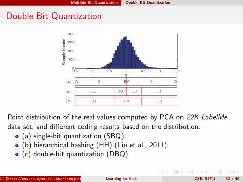
The popular coding strategy SBQ which adopts zero as the thresholdis shown in Figure (a). Due to the thresholding, the intrinsicneighboring structure in the original space is destroyed.The HH strategy (Liu et al., 2011) is shown in Figure (b). If we used(A,B) to denote the Hamming distance between A and B, we canfind that d(A,D) < d(A,C) for HH, which is obviously notreasonable.With our DBQ code, d(A,D) = 2, d(A,B) = d(C,D) = 1, andd(B,C) = 0, which is obviously reasonable to preserve the similarityrelationships in the original space.




Experiment I

Precision-recall curve on 22K LabelMe data set

0 0.2 0.4 0.6 0.8 10

0.2

0.4

0.6

0.8

1

Recall

Pre

cisi

on

SH−SBQSH−HHSH−DBQ

0 0.2 0.4 0.6 0.8 10

0.2

0.4

0.6

0.8

1

Recall

Pre

cisi

on


SH 32 bits SH 64 bits

0 0.2 0.4 0.6 0.8 10

0.2

0.4

0.6

0.8

1

Recall

Pre

cisi

on


0 0.2 0.4 0.6 0.8 10

0.2

0.4

0.6

0.8

1

Recall

Pre

cisi

on


SH 128 bits SH 256 bits




Experiment II

mAP on LabelMe data set

# bits 32 64SBQ HH DBQ SBQ HH DBQ

ITQ 0.2926 0.2592 0.3079 0.3413 0.3487 0.4002SH 0.0859 0.1329 0.1815 0.1071 0.1768 0.2649PCA 0.0535 0.1009 0.1563 0.0417 0.1034 0.1822LSH 0.1657 0.105 0.12272 0.2594 0.2089 0.2577SIKH 0.0590 0.0712 0.0772 0.1132 0.1514 0.1737

# bits 128 256SBQ HH DBQ SBQ HH DBQ

ITQ 0.3675 0.4032 0.4650 0.3846 0.4251 0.4998SH 0.1730 0.2034 0.3403 0.2140 0.2468 0.3468PCA 0.0323 0.1083 0.1748 0.0245 0.1103 0.1499LSH 0.3579 0.3311 0.4055 0.4158 0.4359 0.5154SIKH 0.2792 0.3147 0.3436 0.4759 0.5055 0.5325



Multiple-Bit Quantization Manhattan Quantization

Quantization Stage




Natural Binary Code(NBC)




Manhattan Distance

Let x = [x1, x2, · · · , xd]T , y = [y1, y2, · · · , yd]T , the Manhattan distancebetween x and y is defined as follows:

dm(x,y) =

d∑i=1

|xi − yi|,

where |x| denotes the absolute value of x.




Manhattan Distance Driven Quantization

We divide each projected dimension into 2q regions and then use qbits of natural binary code to encode the index of each region.

For example, If q = 3, the indices of regions are {0, 1, 2, 3, 4, 5, 6, 7}and the natural binary codes are{000, 001, 010, 011, 100, 101, 110, 111}





We divide each projected dimension into 2q regions and then use qbits of natural binary code to encode the index of each region.

For example, If q = 3, the indices of regions are {0, 1, 2, 3, 4, 5, 6, 7}and the natural binary codes are{000, 001, 010, 011, 100, 101, 110, 111}





Manhattan quantization(MQ) with q bits is denoted as q-MQ.

For example, if q = 2,

dm(000100, 110000) = dd(00, 11) + dd(01, 00) + dd(00, 00)

= 3 + 1 + 0

= 4.




Experiment I

0 0.2 0.4 0.6 0.8 10

0.2

0.4

0.6

0.8

1

Recall

Pre

cisi

on

SH SBQSH HQSH 2−MQ

SH 32 bits

0 0.2 0.4 0.6 0.8 10

0.2

0.4

0.6

0.8

1

RecallP

reci

sion


SH 64 bits

0 0.2 0.4 0.6 0.8 10

0.2

0.4

0.6

0.8

1

Recall

Pre

cisi

on


SH 128 bits

0 0.2 0.4 0.6 0.8 10

0.2

0.4

0.6

0.8

1

Recall

Pre

cisi

on


SH 256 bits

0 0.2 0.4 0.6 0.8 10

0.2

0.4

0.6

0.8

1

Recall

Pre

cisi

on

SIKH SBQSIKH HQSIKH 2−MQ

SIKH 32 bits

0 0.2 0.4 0.6 0.8 10

0.2

0.4

0.6

0.8

1

Recall

Pre

cisi

on


SIKH 64 bits

0 0.2 0.4 0.6 0.8 10

0.2

0.4

0.6

0.8

1

Recall

Pre

cisi

on


SIKH 128 bits

0 0.2 0.4 0.6 0.8 10

0.2

0.4

0.6

0.8

1

Recall

Pre

cisi

on


SIKH 256 bits

Figure: Precision-recall curve on 22K LabelMe data set




Experiment II

Table: mAP on ANN SIFT1M data set. The best mAP among SBQ, HQ and2-MQ under the same setting is shown in bold face.

# bits 32 64 96SBQ HQ 2-MQ SBQ HQ 2-MQ SBQ HQ 2-MH

ITQ 0.1657 0.2500 0.2750 0.4641 0.4745 0.5087 0.5424 0.5871 0.6263SIKH 0.0394 0.0217 0.0570 0.2027 0.0822 0.2356 0.2263 0.1664 0.2768LSH 0.1163 0.0961 0.1173 0.2340 0.2815 0.3111 0.3767 0.4541 0.4599SH 0.0889 0.2482 0.2771 0.1828 0.3841 0.4576 0.2236 0.4911 0.5929PCA 0.1087 0.2408 0.2882 0.1671 0.3956 0.4683 0.1625 0.4927 0.5641



Conclusion

Outline




4 Conclusion

5 Reference



Conclusion

Conclusion

Hashing can significantly improve searching speed and reduce storagecost.

Projections with isotropic variances will be better than those withanisotropic variances. (IsoHash)

The quantization stage is at least as important as the projectionstage. (DBQ/MQ)



Conclusion

Q & A

Thanks!

Question?

Code available athttp://www.cs.sjtu.edu.cn/~liwujun




Reference

Outline




4 Conclusion

5 Reference



References

A. Andoni and P. Indyk. Near-optimal hashing algorithms for approximatenearest neighbor in high dimensions. Commun. ACM, 51(1):117–122,2008.

M. Chu. Constructing a Hermitian matrix from its diagonal entries andeigenvalues. SIAM Journal on Matrix Analysis and Applications, 16(1):207–217, 1995.

M. Datar, N. Immorlica, P. Indyk, and V. S. Mirrokni. Locality-sensitivehashing scheme based on p-stable distributions. In Proceedings of theACM Symposium on Computational Geometry, 2004.

A. Gionis, P. Indyk, and R. Motwani. Similarity search in high dimensionsvia hashing. In Proceedings of International Conference on Very LargeData Bases, 1999.

Y. Gong and S. Lazebnik. Iterative quantization: A procrustean approachto learning binary codes. In Proceedings of Computer Vision andPattern Recognition, 2011.

A. Horn. Doubly stochastic matrices and the diagonal of a rotation matrix.American Journal of Mathematics, 76(3):620–630, 1954.



References

W. Kong and W.-J. Li. Double-bit quantization for hashing. InProceedings of the Twenty-Sixth AAAI Conference on ArtificialIntelligence (AAAI), 2012a.

W. Kong and W.-J. Li. Isotropic hashing. In Proceedings of the 26thAnnual Conference on Neural Information Processing Systems (NIPS),2012b.

W. Kong, W.-J. Li, and M. Guo. Manhattan hashing for large-scale imageretrieval. In The 35th International ACM SIGIR conference on researchand development in Information Retrieval (SIGIR), 2012.

B. Kulis and K. Grauman. Kernelized locality-sensitive hashing for scalableimage search. In Proceedings of International Conference on ComputerVision, 2009.

B. Kulis, P. Jain, and K. Grauman. Fast similarity search for learnedmetrics. IEEE Trans. Pattern Anal. Mach. Intell., 31(12):2143–2157,2009.

W. Liu, J. Wang, S. Kumar, and S. Chang. Hashing with graphs. InProceedings of International Conference on Machine Learning, 2011.



Reference

M. Norouzi and D. J. Fleet. Minimal loss hashing for compact binarycodes. In Proceedings of International Conference on Machine Learning,2011.

M. Raginsky and S. Lazebnik. Locality-sensitive binary codes fromshift-invariant kernels. In Proceedings of Neural Information ProcessingSystems, 2009.

J. Wang, S. Kumar, and S.-F. Chang. Sequential projection learning forhashing with compact codes. In Proceedings of International Conferenceon Machine Learning, 2010a.

J. Wang, S. Kumar, and S.-F. Chang. Semi-supervised hashing forlarge-scale image retrieval. In Proceedings of Computer Vision andPattern Recognition, 2010b.

Y. Weiss, A. Torralba, and R. Fergus. Spectral hashing. In Proceedings ofNeural Information Processing Systems, 2008.



Date post:	18-May-2018
Category:	Documents
Upload:	nguyentuong
View:	214 times
Download:	1 times

Learning to Hash with its Application to Big Data ...cs.nju.edu.cn/lwj/slides/hash.pdf · Problem...

Documents