Introduction Baseline Model Simulations Robustness Checks Large Deviations Conclusion Learning to Love Money Tingwen Liu 1 Dennis O’Dea 1 Sergey V. Popov 2 1 Department of Economics University of Illinois 2 Center for Advanced Studies Higher School of Economics, Moscow 8 August 2011
Transcript
Introduction Baseline Model Simulations Robustness Checks Large Deviations Conclusion
Learning to Love Money
Tingwen Liu1 Dennis O’Dea1 Sergey V. Popov2
1Department of EconomicsUniversity of Illinois
2Center for Advanced StudiesHigher School of Economics, Moscow
8 August 2011
Introduction Baseline Model Simulations Robustness Checks Large Deviations Conclusion
Money appeared in a multitude of cultures independently.
Money facilitated trade across the Eurasia and beyond.
We want to study:
Can learning from experience justify the appearance ofinterest in money?
Can learning be used to select an equilibrium of theKiyotaki-Wright model?
Introduction Baseline Model Simulations Robustness Checks Large Deviations Conclusion
Kiyotaki & Wright (1989): when goods become commoditymoney, and when fiat money are good for economy.
Introduction Baseline Model Simulations Robustness Checks Large Deviations Conclusion
Kiyotaki & Wright (1989): when goods become commoditymoney, and when fiat money are good for economy.
Lagos & Wright (2005): endogenized the commodity moneysupply.
Duffy & Ochs (1999): experiment on people — whether theystart playing KW equilibrium.
Ritter (1995): Government “advertizes” money => no moneyis not an equilibrium.
Most important:
Burdett, Trejos and Wright (1999): how people learn to usecommodity money.
Evans and Honkapohja (2001): Learning Dynamics,Stochastic Approximation
Williams (2002): Large Deviations
Our paper: how people learn to use fiat money.
Introduction Baseline Model Simulations Robustness Checks Large Deviations Conclusion
Time is discrete and infinite.
One coin in the economy.
Finite number of agents; they specialize in what they produce.
Goods and coin are indivisible, no storage costs.
Some agents like some other agents’ products.
Agents meet randomly and anonymously each period.
Introduction Baseline Model Simulations Robustness Checks Large Deviations Conclusion
U is utility from consumption of good.
c is disutility from production.
δ is a time discount factor.
p is the probability of mutual coincidence of wants; q is theprobability that only one agent wants the other agent’s good.
p + 2q ≤ 1.
Introduction Baseline Model Simulations Robustness Checks Large Deviations Conclusion
Agents meet in pairs.
Introduction Baseline Model Simulations Robustness Checks Large Deviations Conclusion
Agents meet in pairs.
If agents have mutual coincidence of wants, both of them willtrade with each other (get U).
Introduction Baseline Model Simulations Robustness Checks Large Deviations Conclusion
Agents meet in pairs.
If agents have mutual coincidence of wants, both of them willtrade with each other (get U).
If only one agent wants to trade, they might use money.If desiring agent has money, she’d offer it (offering a coin isfree).If the counteragent accepts money, trade occurs (seller gets acoin; buyer loses a coin and gets U).
If both agents do not want their partner’s good, they willdepart.
At the end of the day, everyone who has no good producesand pays cost c.
Introduction Baseline Model Simulations Robustness Checks Large Deviations Conclusion
Universal Rejection Equilibrium No one takes money — alwaysexists.Universal Acceptance Equilibrium V0 is value of not havingmoney, V1 is value of having a coin.
V ∗
0
δ= p (V ∗
0 + U − c) +1
n − 1q (V ∗
1 − c) +
(1 − p −
qn − 1
)(V ∗
0 )
V ∗
1
δ= p (V ∗
1 + U − c) + q (V ∗
0 + U) + (1 − p − q) (V ∗
1 )
Introduction Baseline Model Simulations Robustness Checks Large Deviations Conclusion
This is an equilibrium when V ∗
1 − V ∗
0 = V ∗
∆ > c.
V∆ = V ∗
1 − V ∗
0 =qU + q
n−1 c1δ− 1 + qn
n−1
⇒ δ >c
qU + (1 − q)c
Introduction Baseline Model Simulations Robustness Checks Large Deviations Conclusion
Adaptive Learning
Agents have a belief about value of money V .
...start with belief of 0.
...updating: if agenttook money at period T1;successfully traded it at moment T2;at beginning of period T2 + 1 agent’s V becomesγ(δT2−T1U) + (1 − γ)V .
Agents make a decision implementation error with probabilityε.
γ: Gain
ε: Error probability
Introduction Baseline Model Simulations Robustness Checks Large Deviations Conclusion
Beliefs follow the following dynamics:
Vt+1 = Vt + γ(δτ U − Vt)
Where τ is the random wait time until successful trade. It isessentially an exponential wait time, depending on everyone’sacceptance rules and the error probabilities.Note that the time scale t refers to learning time.
Introduction Baseline Model Simulations Robustness Checks Large Deviations Conclusion
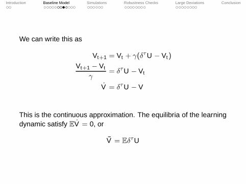
We can write this as
Vt+1 = Vt + γ(δτ U − Vt)
Vt+1 − Vt
γ= δτ U − Vt
V = δτ U − V
This is the continuous approximation. The equilibria of the learningdynamic satisfy EV = 0, or
V = Eδτ U
Introduction Baseline Model Simulations Robustness Checks Large Deviations Conclusion
There are two such equilibria:
Under universal acceptance, the wait time τ can beapproximated by an exponential distribution with wait time qε,leading to equilibria value of money
δqε
1 − δ(1 − qε)
Under universal rejection, the wait time is is given by q(1 − ε),with value
δq(1 − ε)
1 − δ(1 − q(1 − ε))
These correspond exactly to the rational equilibria.
Introduction Baseline Model Simulations Robustness Checks Large Deviations Conclusion
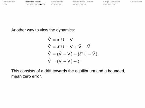
Another way to view the dynamics:
V = δτ U − V
V = δτ U − V + V − V
V = (V − V ) + (δτ U − V )
V = (V − V ) + ξ
This consists of a drift towards the equilibrium and a bounded,mean zero error.
Introduction Baseline Model Simulations Robustness Checks Large Deviations Conclusion
The dynamics of learning around the equilibria are described bythe mean dynamics of the learning algorithm:
˙V = E((V − V ) − ξ)
˙V = (V − V )
˙V = 0 at V = V
That is, both equilibria are stochastically stable.
Introduction Baseline Model Simulations Robustness Checks Large Deviations Conclusion
So, learning by itself does not select among rational equilibria;both equilibria can be learned.
So long as errors are possible (ε > 0) and agents learn fromthe past (γ > 0), the learning dynamic will spend some timein both equilibria as t → ∞.
But, it may be possible to characterize how much time in each andhow difficult it is to leave each equilibrium.
Introduction Baseline Model Simulations Robustness Checks Large Deviations Conclusion
We did 1000 simulations for 100 thousand periods, to get a senseof the behavior of the learning dynamic.We use these values for the simulations:
δ = 0.95.
U = 1.
c = 0.1.
γ = 0.2.
ε = 1/200.
Introduction Baseline Model Simulations Robustness Checks Large Deviations Conclusion
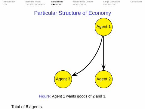
Particular Structure of Economy
Agent 1
Agent 3 Agent 2
Figure: Agent 1 wants goods of 2 and 3.
Total of 8 agents.
Introduction Baseline Model Simulations Robustness Checks Large Deviations Conclusion
Agent 1
Agent 4 Agent 3 Agent 2
Figure: Agent 2 wants goods of 3 and 4.
Total of 8 agents.
Introduction Baseline Model Simulations Robustness Checks Large Deviations Conclusion
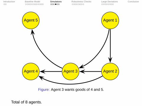
Agent 5 Agent 1
Agent 4 Agent 3 Agent 2
Figure: Agent 3 wants goods of 4 and 5.
Total of 8 agents.
Introduction Baseline Model Simulations Robustness Checks Large Deviations Conclusion
0 2 4 6 8 10
x 104
0
0.1
0.2
0.3
0.4
0.5
0.6
0.7
0.8
0.9
Time, periods
Bel
ief i
n va
lue
of m
oney
MedianMean
Figure: Mean Behavior of Learning.
Introduction Baseline Model Simulations Robustness Checks Large Deviations Conclusion
There is 185 observations of V > c going to V < c.
There is 7787 observations of V < c going to V > c.
These are not necessarily good estimates of equilibriumprobabilities; these are extremely unlikely tail events
Introduction Baseline Model Simulations Robustness Checks Large Deviations Conclusion
Assume agent 8 never ever ever accepts money.
It will slow down learning of agent 7: he has only one channelfor outflow of money.
It will slow down learning of agent 5: he has to deal with agent7.
Will it prevent learning?
Will it be strategically optimal?
Naturally, if both agents 7 and 8 never accepted money, moneywould never circulate.
Introduction Baseline Model Simulations Robustness Checks Large Deviations Conclusion
1 2 3 4 5 6
x 104
0
0.1
0.2
0.3
0.4
0.5
0.6
0.7
0.8
0.9
Time, periods
Bel
ief i
n va
lue
of m
oney
Baseline medianBaseline meanMedian for Agent 1Median for Agent 4Median for Agent 7Mean for Agent 1Mean for Agent 4Mean for Agent 7
Figure: Mean Behavior of Learning.
Introduction Baseline Model Simulations Robustness Checks Large Deviations Conclusion
Assume agent 8 always accepts money.
It will speed up learning of agent 7: he has one channel thatwill always take money.
It will speed up learning of agent 5: he can deal with agent 7.
Will it expedite total learning?
Will it be strategically optimal?
Introduction Baseline Model Simulations Robustness Checks Large Deviations Conclusion
0.2 0.4 0.6 0.8 1 1.2 1.4 1.6 1.8 2
x 104
0
0.1
0.2
0.3
0.4
0.5
0.6
0.7
0.8
0.9
Time, periods
Bel
ief i
n va
lue
of m
oney
Baseline medianBaseline meanMedian for Agent 1Median for Agent 4Median for Agent 7Mean for Agent 1Mean for Agent 4Mean for Agent 7
Figure: Mean Behavior of Learning.
Introduction Baseline Model Simulations Robustness Checks Large Deviations Conclusion
0 0.02 0.04 0.06 0.08 0.1 0.120.02
0.04
0.06
0.08
0.1
0.12
0.14
0.16
Current belief in money value
Pro
babi
lity
of u
sing
mon
ey n
ext p
erio
d
Both counteragents do not use money
Figure: Your Counteragents Do Not Take Money.
Introduction Baseline Model Simulations Robustness Checks Large Deviations Conclusion
0 0.02 0.04 0.06 0.08 0.1 0.120.9
0.92
0.94
0.96
0.98
1
Current belief in money value
Pro
babi
lity
of u
sing
mon
ey n
ext p
erio
d
One of two counteragents is using moneyBoth counteragents use money
Figure: Your Counteragents Take Money.
Introduction Baseline Model Simulations Robustness Checks Large Deviations Conclusion
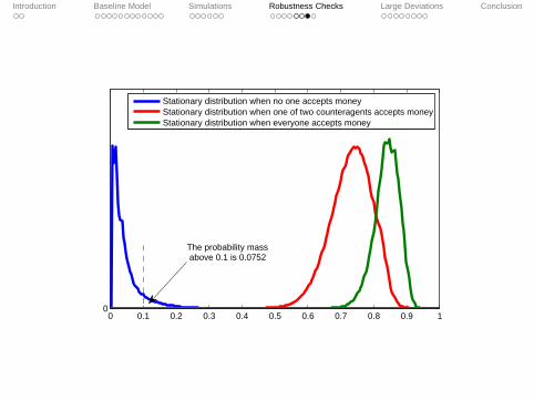
0 0.1 0.2 0.3 0.4 0.5 0.6 0.7 0.8 0.9 10
Stationary distribution when no one accepts moneyStationary distribution when one of two counteragents accepts moneyStationary distribution when everyone accepts money
The probability massabove 0.1 is 0.0752
Introduction Baseline Model Simulations Robustness Checks Large Deviations Conclusion
It is easy to learn to accept money even when no one elsedoes (probability of 7.52% in our parametrization).
It is not easy to become disappointed in money:
Hitting value 0.8 0.7 0.6 0.5Time to achieve 535 40K 51M >2B
Introduction Baseline Model Simulations Robustness Checks Large Deviations Conclusion
How to escape equilibrium
Consider the mean dynamics, holding every other agent’s beliefsfixed:
˙V = (V − V )
In order for V to leave this equilibrium, forcing errors s(t) mustovercome the drift towards V .
Introduction Baseline Model Simulations Robustness Checks Large Deviations Conclusion
How to escape equilibrium
Consider the mean dynamics, holding every other agent’s beliefsfixed:
˙V = (V − V )
In order for V to leave this equilibrium, forcing errors s(t) mustovercome the drift towards V .
With enough lucky (or unlucky) trading experiences, hisestimate of the value of money may leave the equilibrium andchange his acceptance rule.
We solve for the most likely way for this to happen.
Introduction Baseline Model Simulations Robustness Checks Large Deviations Conclusion
The large deviations of these dynamics describe how beliefsescape these equilibria:
it is unlikely, but must eventually happen due to the noise ξ;
if every agent’s beliefs move across the production cost c,they will have moved form the universal rejection equilibriumto the universal acceptance equilibrium.
So we solve for the rate function that governs the likelihood of thathappening.
Introduction Baseline Model Simulations Robustness Checks Large Deviations Conclusion
The large deviation properties are entirely driven by the behavior ofthis random variable:
Z = δτ U, τ ∽ Exponential(λ)
where λ is the probability of trading at equilibrium.
Introduction Baseline Model Simulations Robustness Checks Large Deviations Conclusion
The distribution g(z) of this random variable is given by
g(z) = −λ
(zU
)−1− λ
log δ
U log δ.
for z ∈ [0, U]; essentially a truncated power-law.The distribution of the mean zero error ξ is simply a shift of thisdistribution.
Introduction Baseline Model Simulations Robustness Checks Large Deviations Conclusion
From this we calculate the culmulant generating function:
H(t) = log Ezetz ,
and the rate function I(x) is the Legendre transform of H:
I(x) = supt
xt − H(t).
This function I governs the large deviation properties of Z .
Punchline: I is asymmetric; it is easier to to increase thandecrease, easier to learn money has value than to learn it does
not.
Introduction Baseline Model Simulations Robustness Checks Large Deviations Conclusion
The rate function I at the Universal Acceptance and UniversalRejection equilibria:
0.2 0.4 0.6 0.8 1.0
2
4
6
8
10
12
Figure: Solid - High Value Rate Function. Dashed - Low Value RateFunction
They are zero at their equilibrium.
Introduction Baseline Model Simulations Robustness Checks Large Deviations Conclusion
Superimposed, the difference is clear:
0.2 0.4 0.6 0.8 1.0
5
10
15
20
Figure: Solid - High Value Rate Function. Dashed - Low Value RateFunction
It is much lower cost to escape the low equilibrium.
Introduction Baseline Model Simulations Robustness Checks Large Deviations Conclusion
To characterize the long run distribution over equilibria, considerfirst a single agent leaving the universal rejection equilibrium.To do so, we must find a sequence of trading shocks s(t) (whichhave distribution ξ) that will drive his estimate from V to c at timeT :
V (0) = V
V (T ) = c
V = (V − V (t)) + s(t)
This condition has ODE form:
c = V + eT∫ T
0e−t(V + s(t))dt
Introduction Baseline Model Simulations Robustness Checks Large Deviations Conclusion
We now solve the following minimization problem:
minT ,s(·)
∫ T
0I(s(t))dt
subject to
c = V + eT∫ T
0e−t(V + s(t))dt
The rate function I can be interpreted as the “cost” of a shock ofsize s(t), and we seek shocks of minimal cost that will force thisagent across the boundary c.This is the mostly likely way to escape the equilibrium, thedominant escape path.
Introduction Baseline Model Simulations Robustness Checks Large Deviations Conclusion
The optimal shocks are constant in size. There are two effects:
after you move closer to the boundary, you have lessremaining distance to travel;
but the drift back towards equilibrium is stronger.
The optimal shocks to travel to the boundary in time T is given by
s(t) =eT (V − c)
eT − 1
which is constant in t .
Introduction Baseline Model Simulations Robustness Checks Large Deviations Conclusion
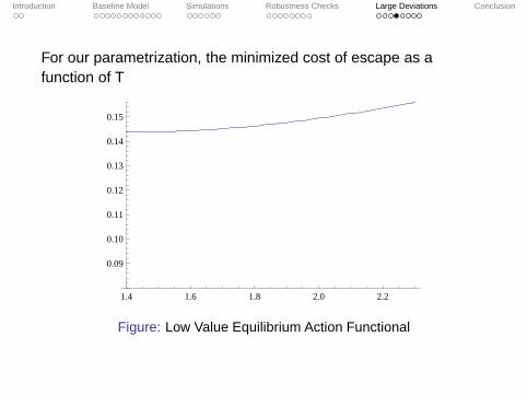
For our parametrization, the minimized cost of escape as afunction of T
1.4 1.6 1.8 2.0 2.2
0.09
0.10
0.11
0.12
0.13
0.14
0.15
Figure: Low Value Equilibrium Action Functional
Introduction Baseline Model Simulations Robustness Checks Large Deviations Conclusion
1.6 1.8 2.0 2.2
20
22
24
26
Figure: High Value Equilibrium Action Functional
There are two ways to escape: larger shocks alow one to escapein a shorter time, but are more costly. For the low equilibrium,since shocks are not so costly, the optimal T is smaller.
Introduction Baseline Model Simulations Robustness Checks Large Deviations Conclusion
c = 0.1 Escape Time Cost ProbabilityLow Value Equilibrium 1.45098 0.143836 0.49438
High Equilibrium 2.14218 18.1264 4.35614E − 40
Introduction Baseline Model Simulations Robustness Checks Large Deviations Conclusion
c = 0.1 Escape Time Cost ProbabilityLow Value Equilibrium 1.45098 0.143836 0.49438
High Equilibrium 2.14218 18.1264 4.35614E − 40Note: this is not an artifact of c being closer to the Low equilibriumthan to the High; with c equidistant we have
c=0.408 Escape Time Cost ProbabilityLow Value Equilibrium 0.857147 2.42028 5.55163E − 6
High Equilibrium 1.63005 4.14184 1.01415E − 9It is driven by asymmetry in the escape probabilities.
Introduction Baseline Model Simulations Robustness Checks Large Deviations Conclusion
c = 0.1 Escape Time Cost ProbabilityLow Value Equilibrium 1.45098 0.143836 0.49438
High Equilibrium 2.14218 18.1264 4.35614E − 40Note: this is not an artifact of c being closer to the Low equilibriumthan to the High; with c equidistant we have
c=0.408 Escape Time Cost ProbabilityLow Value Equilibrium 0.857147 2.42028 5.55163E − 6
High Equilibrium 1.63005 4.14184 1.01415E − 9It is driven by asymmetry in the escape probabilities. Probabilitiesare equal at c ≈ 0.461.
Introduction Baseline Model Simulations Robustness Checks Large Deviations Conclusion
To calculate the probability of the system as whole escapingequilibrium, there are only two ways for an agent to leave oneequilibrium:
In the manner described above, on his own - this is costly
If enough of his trading partners escape as above, the ODEgoverning his learning flips, so that the other equilibrium isattractive, and everyone may follow his new mean dynamics -this has cost zero.
We solve for the cost minimizing combination of agents going tothe boundary on their own and “waiting” while other follow zerocost mean dynamics.
Introduction Baseline Model Simulations Robustness Checks Large Deviations Conclusion
For our parametrization, the “low cost” way to escape the lowequilibrium is for half to escape, half to wait. To escape the highequilibrium all agents must escape on their own. This is very costly.
Transition CostLow Value Equilibrium 0.594863
High Equilibrium 145.011
Theorem (Williams 2002)As the gain γ → 0, the invariant distribution of beliefs areconcentrated on the higher-cost equilibrium
Introduction Baseline Model Simulations Robustness Checks Large Deviations Conclusion
Conclusion
We propose a way to choose a rational equilibrium in theKiyotaki and Wright model.
Introduction Baseline Model Simulations Robustness Checks Large Deviations Conclusion
Conclusion
We propose a way to choose a rational equilibrium in theKiyotaki and Wright model.
We show that the “good” rational equilibrium is quiteprominent.
In fact, it is the long run dominant equilibrium as γ → 0.