Learning your Child’s Price Evidence from Data on Projected Dowry in Rural India A. V. CHARI AND ANNEMIE MAERTENS WR-899 November 2011 This paper series made possible by the NIA funded RAND Center for the Study of Aging (P30AG012815) and the NICHD funded RAND Population Research Center (R24HD050906). WORKING P A P E R This product is part of the RAND Labor and Population working paper series. RAND working papers are intended to share researchers’ latest findings and to solicit informal peer review. They have been approved for circulation by RAND Labor and Population but have not been formally edited or peer reviewed. Unless otherwise indicated, working papers can be quoted and cited without permission of the author, provided the source is clearly referred to as a working paper. RAND’s publications do not necessarily reflect the opinions of its research clients and sponsors. is a registered trademark.
Transcript
Learning your Child’s Price
Evidence from Data on Projected Dowry in Rural India
A. V. CHARI AND ANNEMIE MAERTENS
WR-899
November 2011
This paper series made possible by the NIA funded RAND Center for the Study of Aging (P30AG012815) and the NICHD funded RAND Population Research Center (R24HD050906).
WORK ING P A P E R
This product is part of the RAND Labor and Population working paper series. RAND working papers are intended to share researchers’ latest findings and to solicit informal peer review. They have been approved for circulation by RAND Labor and Population but have not been formally edited or peer reviewed. Unless otherwise indicated, working papers can be quoted and cited without permission of the author, provided the source is clearly referred to as a working paper. RAND’s publications do not necessarily reflect the opinions of its research clients and sponsors.
is a registered trademark.
Number of households in village 1,720Number of households in sample 339Number of married children1 119Number of unmarried children1 719Average age of married children 21Average age of unmarried children 11Average number of household members 5.55Average Kharif income (Rs)2 51,176Average education level of respondent (in years)3 4.77Average dowry willing to accept (boys) (Rs)4 70,671Average dowry willing to pay (girls) (Rs)4 79,130Average dowry willing to accept (boys) (Rs)4 50,000Average dowry willing to pay (girls) (Rs)4 50,000
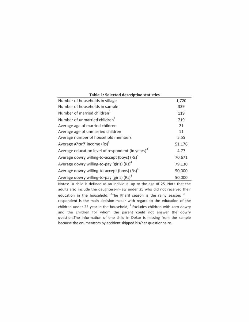
Table 1: Selected descriptive statistics
Notes: 1A child is defined as an individual up to the age of 25. Note that theadults also include the daughters in law under 25 who did not received theireducation in the household; 2The Kharif season is the rainy season; 3
respondent is the main decision maker with regard to the education of thechildren under 25 year in the household; 4 Excludes children with zero dowryand the children for whom the parent could not answer the dowryquestion.The information of one child in Dokur is missing from the samplebecause the enumerators by accident skipped his/her questionnaire.
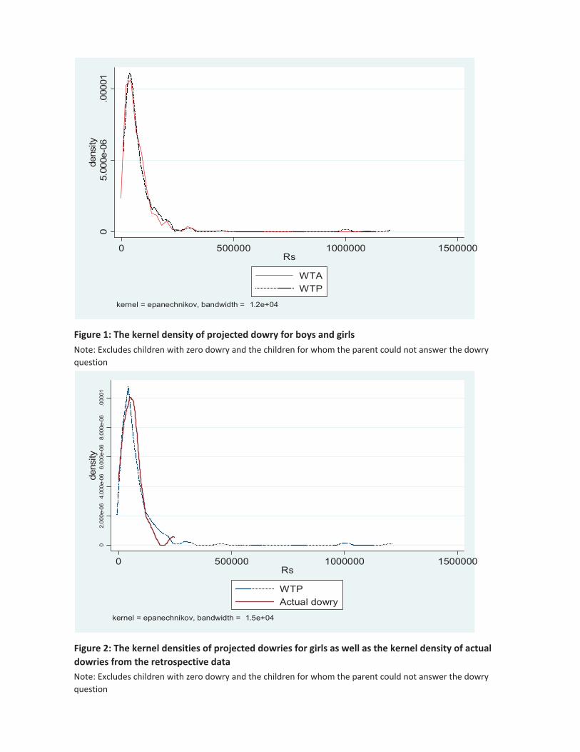
Figure 1: The kernel density of projected dowry for boys and girls
Figure 2: The kernel densities of projected dowries for girls as well as the kernel density of actualdowries from the retrospective dataNote: Excludes children with zero dowry and the children for whom the parent could not answer the dowryquestion
Note: Excludes children with zero dowry and the children for whom the parent could not answer the dowryquestion
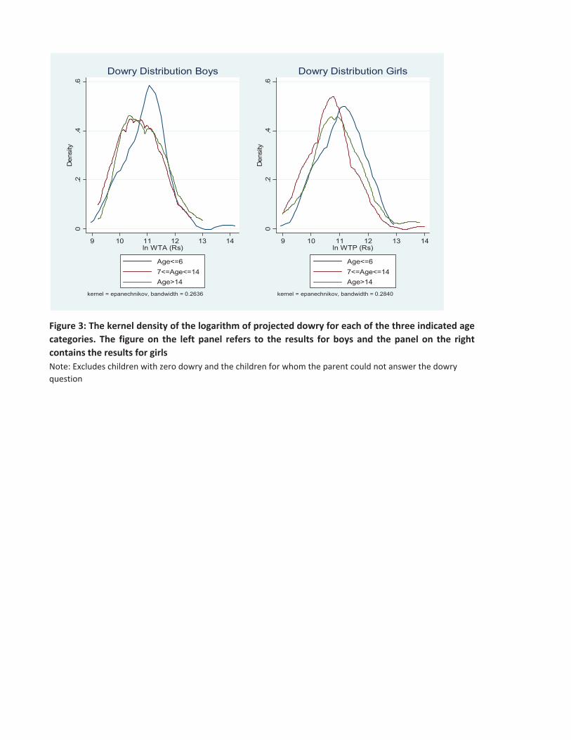
Figure 3: The kernel density of the logarithm of projected dowry for each of the three indicated agecategories. The figure on the left panel refers to the results for boys and the panel on the rightcontains the results for girlsNote: Excludes children with zero dowry and the children for whom the parent could not answer the dowryquestion
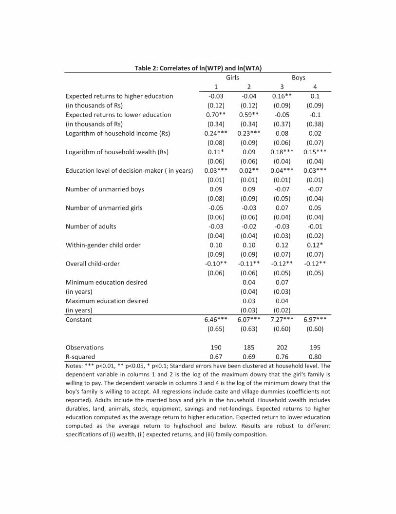
1 2 3 4Expected returns to higher education 0.03 0.04 0.16** 0.1(in thousands of Rs) (0.12) (0.12) (0.09) (0.09)Expected returns to lower education 0.70** 0.59** 0.05 0.1(in thousands of Rs) (0.34) (0.34) (0.37) (0.38)Logarithm of household income (Rs) 0.24*** 0.23*** 0.08 0.02
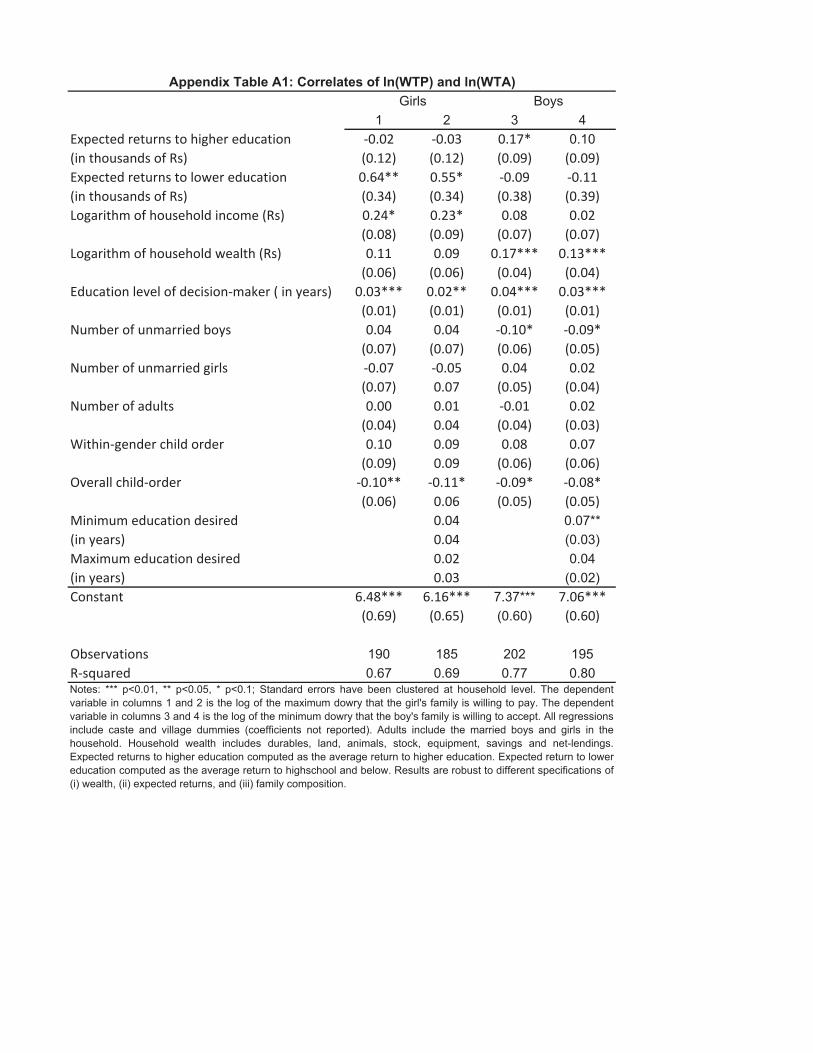
Table 2: Correlates of ln(WTP) and ln(WTA)Girls Boys
Notes: *** p<0.01, ** p<0.05, * p<0.1; Standard errors have been clustered at household level. Thedependent variable in columns 1 and 2 is the log of the maximum dowry that the girl's family iswilling to pay. The dependent variable in columns 3 and 4 is the log of the minimum dowry that theboy's family is willing to accept. All regressions include caste and village dummies (coefficients notreported). Adults include the married boys and girls in the household. Household wealth includesdurables, land, animals, stock, equipment, savings and net lendings. Expected returns to highereducation computed as the average return to higher education. Expected return to lower educationcomputed as the average return to highschool and below. Results are robust to differentspecifications of (i) wealth, (ii) expected returns, and (iii) family composition.
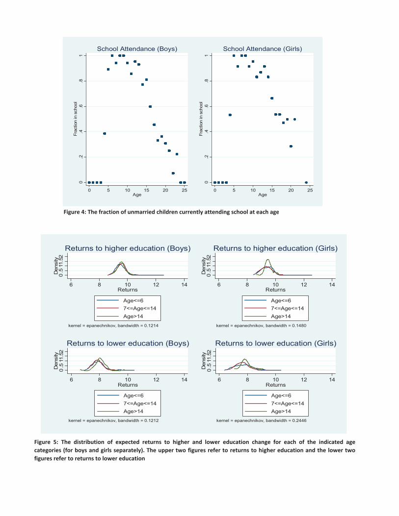
Figure 4: The fraction of unmarried children currently attending school at each age
Figure 5: The distribution of expected returns to higher and lower education change for each of the indicated agecategories (for boys and girls separately). The upper two figures refer to returns to higher education and the lower twofigures refer to returns to lower education
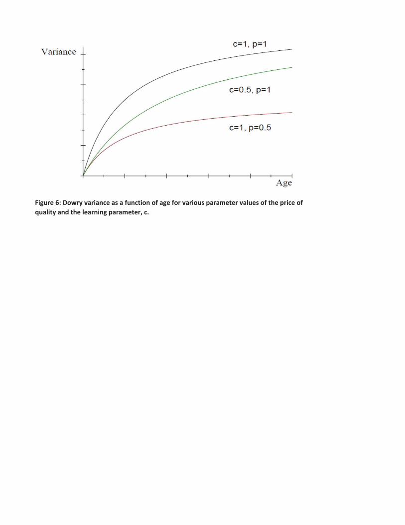
Figure 6: Dowry variance as a function of age for various parameter values of the price ofquality and the learning parameter, c.
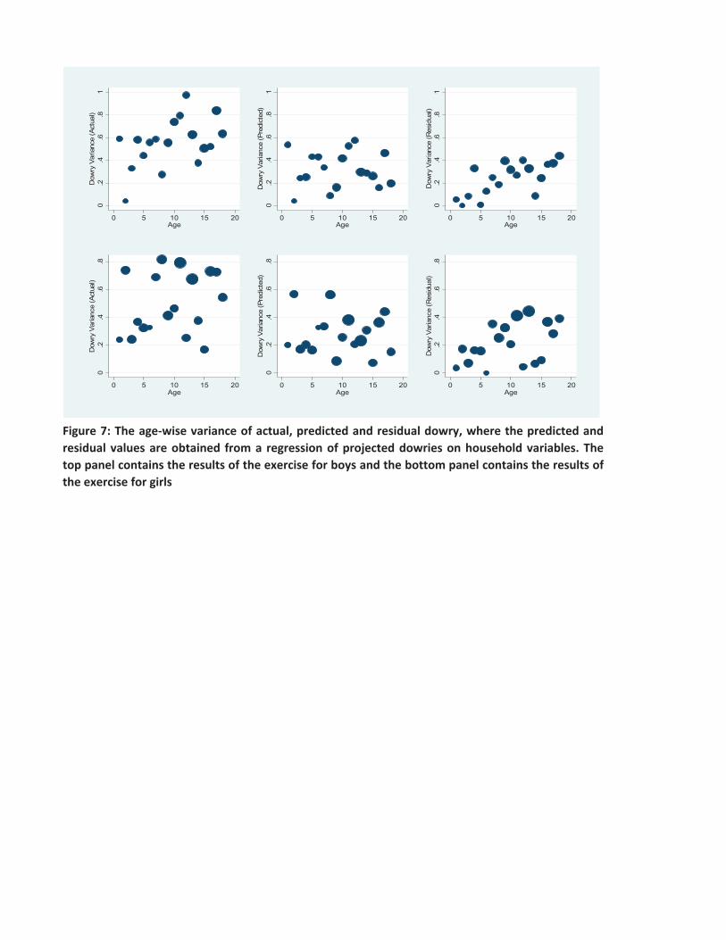
Figure 7: The age wise variance of actual, predicted and residual dowry, where the predicted andresidual values are obtained from a regression of projected dowries on household variables. Thetop panel contains the results of the exercise for boys and the bottom panel contains the results ofthe exercise for girls
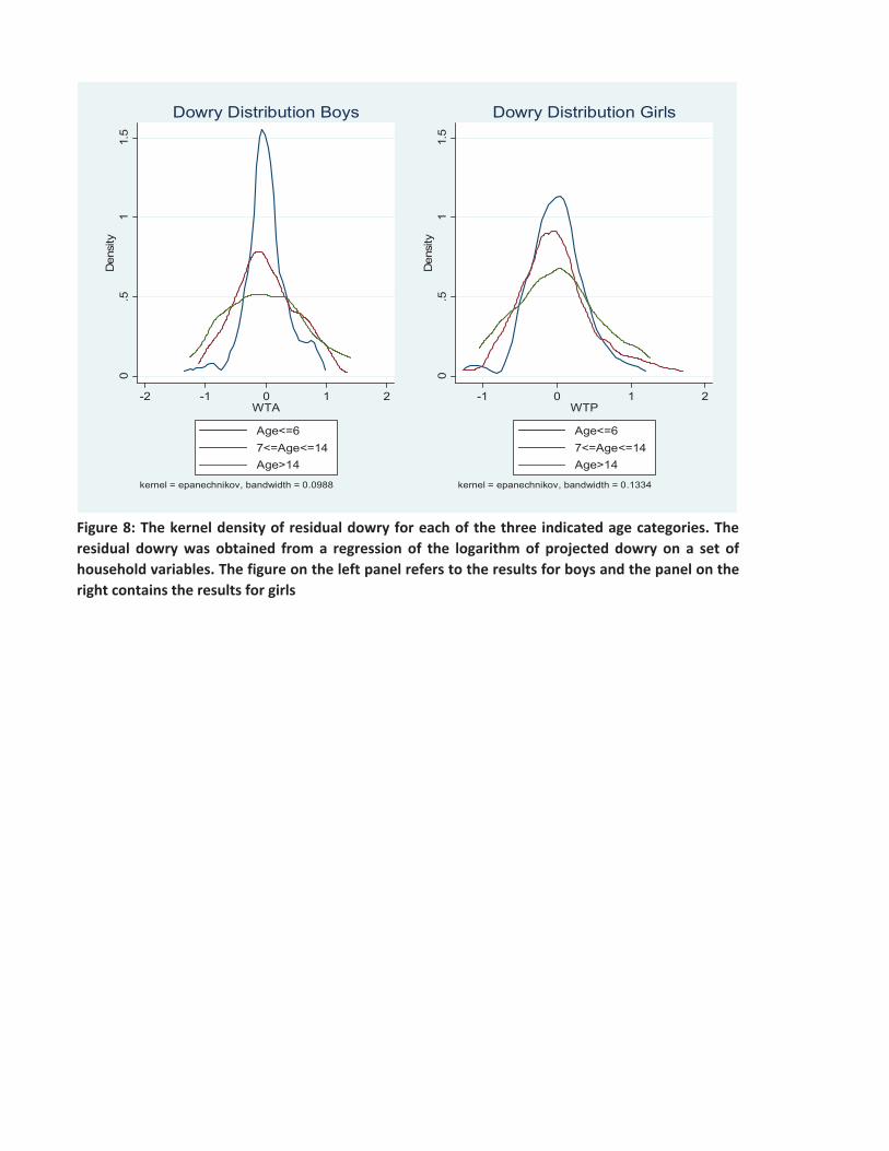
Figure 8: The kernel density of residual dowry for each of the three indicated age categories. Theresidual dowry was obtained from a regression of the logarithm of projected dowry on a set ofhousehold variables. The figure on the left panel refers to the results for boys and the panel on theright contains the results for girls
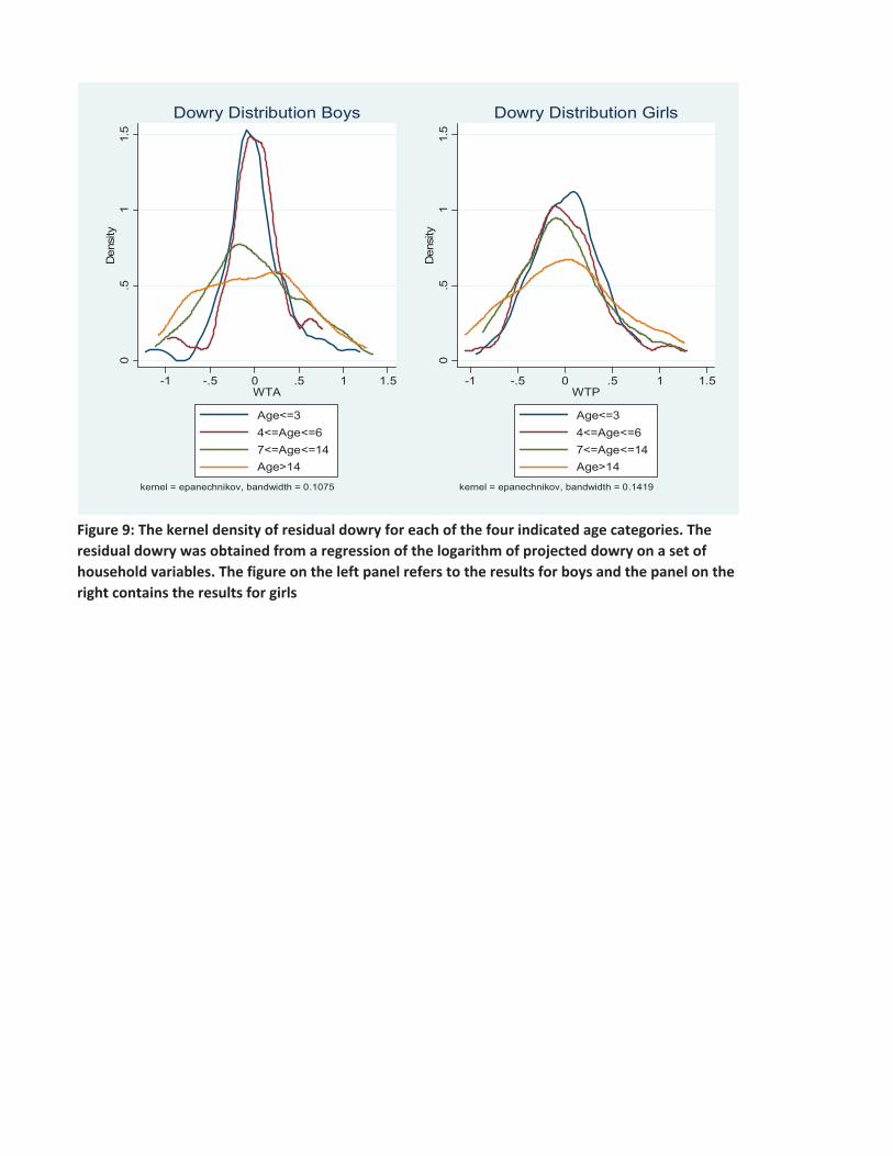
Figure 9: The kernel density of residual dowry for each of the four indicated age categories. Theresidual dowry was obtained from a regression of the logarithm of projected dowry on a set ofhousehold variables. The figure on the left panel refers to the results for boys and the panel on theright contains the results for girls
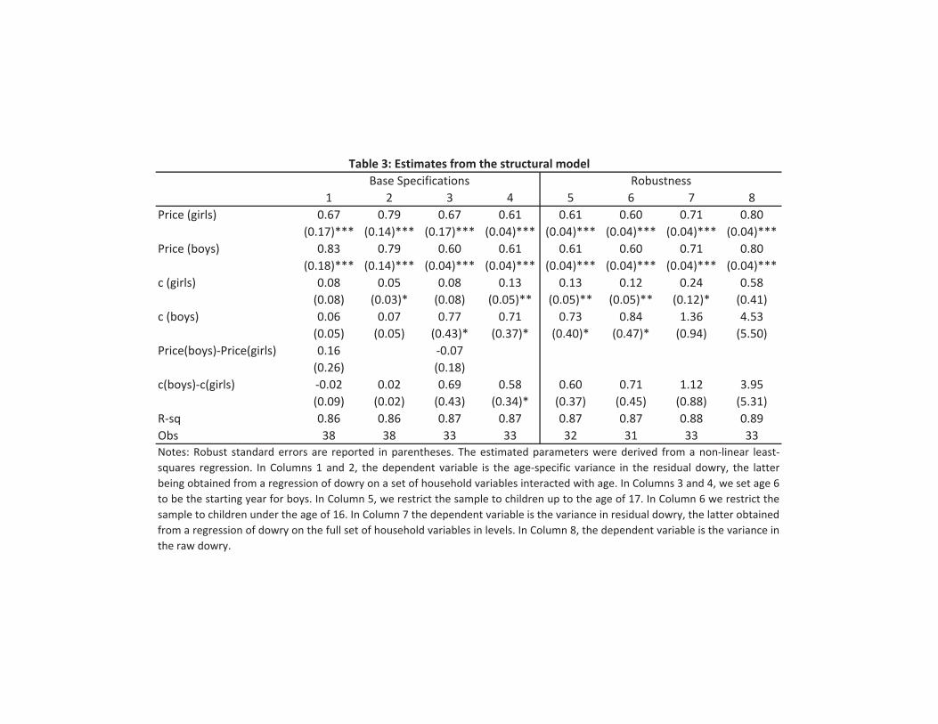
Table 3: Estimates from the structural modelBase Specifications Robustness
Notes: Robust standard errors are reported in parentheses. The estimated parameters were derived from a non linear leastsquares regression. In Columns 1 and 2, the dependent variable is the age specific variance in the residual dowry, the latterbeing obtained from a regression of dowry on a set of household variables interacted with age. In Columns 3 and 4, we set age 6to be the starting year for boys. In Column 5, we restrict the sample to children up to the age of 17. In Column 6 we restrict thesample to children under the age of 16. In Column 7 the dependent variable is the variance in residual dowry, the latter obtainedfrom a regression of dowry on the full set of household variables in levels. In Column 8, the dependent variable is the variance inthe raw dowry.
Expected returns to higher education 0.02 0.03 0.17*(in thousands of Rs) (0.12) (0.12) (0.09) (0.09)Expected returns to lower education 0.64** 0.55* 0.09 0.11(in thousands of Rs) (0.34) (0.34) (0.38) (0.39)Logarithm of household income (Rs) 0.24* 0.23* 0.08 0.02