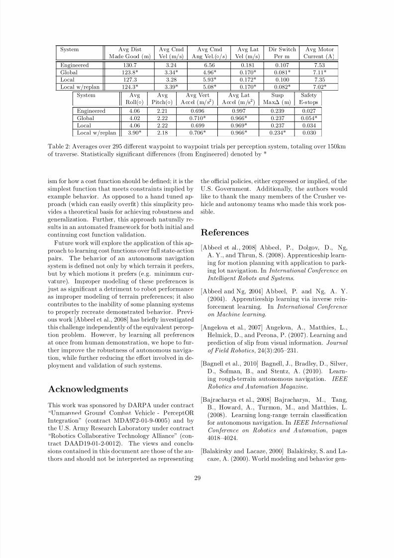
learningFromDemoIJRR2010

8/6/2019 learningFromDemoIJRR2010

http://slidepdf.com/reader/full/learningfromdemoijrr2010 1/32

Learning from Demonstration for Autonomous Navigation in

Complex Unstructured Terrain

David Silver, J. Andrew Bagnell, Anthony Stentz

Carnegie Mellon University

Pittsburgh, PA, USA

June 24, 2010

Abstract

Rough terrain autonomous navigation continues topose a challenge to the robotics community. Robustnavigation by a mobile robot depends not only on

the individual performance of perception and plan-ning systems, but on how well these systems are cou-pled. When traversing complex unstructured terrain,this coupling (in the form of a cost function) has alarge impact on robot behavior and performance, ne-cessitating a robust design. This paper explores theapplication of Learning from Demonstration to thistask for the Crusher autonomous navigation plat-form. Using expert examples of desired navigationbehavior, mappings from both online and offline per-ceptual data to planning costs are learned. Chal-lenges in adapting existing techniques to complex on-line planning systems and imperfect demonstrationare addressed, along with additional practical consid-erations. The benefits to autonomous performance of this approach are examined, as well as the decreasein necessary designer effort. Experimental results arepresented from autonomous traverses through com-plex natural environments.

1 Introduction

The capability of autonomous robotic systems to suc-cessfully navigate through difficult environments con-

tinues to advance [Kelly et al., 2006, Buehler, 2006].Ever improving high resolution sensors and percep-tion algorithms allow a mobile robot to build a de-tailed model of its environment, and advances in plan-ning systems allow for the generation of ever morecomplex routes and trajectories towards achieving anavigation goal. However, as perception and plan-ning systems become more complex, so does the taskof coupling these systems.

A common division of responsibility in mobile

robotics tasks a perception system with construct-ing a discrete model of the environment. This modelis then interpreted into an appropriate form for useby a planning system, which determines the robot’sactions. In the simplest case, this interpretation de-termines which locations in the environment modelthe robot can and cannot traverse through (i.e. anobstacle versus freespace or traversable versus non-traversable distinction). A planning system thencomputes a path through traversable regions of theenvironment. In this way, perception and planningare coupled through a binary classification of the en-vironment.

While such a binary approach was utilized inthe early days of outdoor autonomous navigation[Olin and Tseng, 1991], more recent work of the pastdecade has shown it to be insufficient for navigating

complex unstructured environments. Rough naturalterrain is not easily partitioned into clear traversableand non-traversable classes; while certain objectsmay be obvious non-traversable obstacles, unstruc-tured environments generally present a continuum of terrain that could fall into the traversable categorysuch as steep slopes, ditches, smaller (surmountable)objects, and widely varying vegetation (Figure 1).A binary interpretation results in no distinction be-tween these different terrain features, resulting in be-havior that is either overly aggressive or conservative(Figure 2).

As these issues have become better under-

stood, the result has been a move to sys-tems that use a continuous coupling betweenperception and planning [Kelly et al., 2006,Lacaze et al., 2002, Stentz et al., 2007,Singh et al., 2000, Urmson et al., 2006,Biesiadecki and Maimone, 2006]. Such a cou-pling is commonly called a Cost Function . A costfunction maps terrain features produced by percep-tion to a scalar cost value, with lower cost terrainbeing preferable to higher cost terrain. A planning

1



system then computes a trajectory that minimizesthe accrued cost of traversed terrain.

While using a continuous definition of cost allowsfor more intelligent behavior, it also increases thecomplexity of deploying a properly functioning robot.Systems that used a traversable or non-traversable

distinction only had to solve a binary classificationproblem. This mapping completely determined thebehavior of the robot (with respect to where it pre-ferred to drive); essentially, the desired behavior of the robot was encoded in the classification func-tion mapping perceptual data to traversable or non-traversable. However, in a system with continuouscosts, in essence a full regression problem must besolved. That is, the desired behavior of a robot isencoded not in a mapping from terrain properties toa binary class, but in a mapping from terrain prop-erties to a scalar value that encodes preferences (seeFigure 2).

This mapping from terrain properties to cost isfar more complex than a binary mapping, as it en-codes far more complex behavior (through continu-ous output). Worse, the preferences amongst terraintypes are not always well understood, because themetric for performance is rarely concretely defined.Common metrics for autonomous behavior includemaximizing safety or probability of success, minimiz-ing distance traveled or time taken, minimizing netenergy loss, minimizing observability or maximizingsensor coverage. However, often the actual desiredrobot behavior optimizes a combination of such met-rics; for example, it may be desirable for a robot toapproximately maximize safety but take certain risksto minimize distance traveled. Encoding a single met-ric into a cost function is sufficiently difficult, butproperly inferring the correct weighting to constructa multi-criterion optimization problem is even moredaunting. Fundamentally, while humans are good atdriving in complex or off-road environments, they arenot good at articulating their preferences in doing so.

Therefore, as preferences that mobile robotic sys-tems are expected to exhibit become more complex,the task of encoding these preferences in a cost func-tion will become both more difficult and time con-

suming, while at the same time becoming more cen-tral to improving performance. Unfortunately, thischallenge has not received a great deal of focus; it isoften only briefly mentioned in the literature. Withrespect to costs defined over patches of terrain, themapping to cost from terrain parameters or featuresis rarely described in detail, usually with the state-ment that it was simply constructed and hand-tunedto provide good empirical performance.

The issue of cost function design and tuning

was central during the development of Crusher[Stentz et al., 2007, Bagnell et al., 2010](Figure 1), avehicle designed from scratch for off-road autonomousmobility. Crusher is capable of traversing steepslopes, deep washes and ditches, large boulders, anddense vegetation. Robust navigation through such

terrain requires a proper description of preferencesover such terrain (e.g. how far should Crusher travelthrough dense vegetation to avoid a small ditch).Complicating matters further is the complexity of theperceptual inputs that navigating such environmentsnecessitates; complex terrain requires a high dimen-sional description in order to sufficiently encode allthe relevant features (see Figure 3). Finally, Crusherreceives multiple sources of perceptual input: alongwith the ever changing stream of perceptual dataproduced onboard the vehicle, static prior data wasavailable at varying resolution over large areas of op-eration (potentially hundreds of square kilometers)

[Silver et al., 2006, Silver et al., 2008]. This necessi-tated multiple cost functions for interpreting thesedisjoint data sources that encoded robust behaviorboth individually and when fused together.

This paper explores the application of a learn-ing from demonstration approach to this challenge.Specifically, algorithms are presented for learninggeneralizable terrain cost functions from expertdemonstration of desired behavior. This approachcan both reduce development effort and improve per-formance when applied to mobile robotic systems.The next section provides a brief overview of pre-vious and related work in coupling perception and

planning systems through cost functions. Section 3presents the basic theory of our approach, and Sec-tion 4 describes its practical adaptation to mobilerobotics. Experimental results from the Crusher sys-tem are provided in Section 5, with discussion andconclusion in Section 6.

2 Related Work

2.1 Hand Tuned Cost Functions

Manual hand tuning and engineering has by far been

the most common approach to constructing costfunctions for mobile robotic systems. Often, this isdone with little or no formalism; cost function designby hand remains one of the ’black arts’ of mobilerobotics, and has been applied to untold numbers of robotic systems. However, there has previously beenwork that created reusable frameworks for manualdesign and tuning of cost functions to map perceptualfeatures into scalar costs [Stentz and Hebert, 1995,Singh et al., 2000, Balakirsky and Lacaze, 2000,

2



Figure 1: The Crusher autonomous mobility platform is capable of cross-country traverse through rough,complex, and unstructured terrain

Seraji and Howard, 2002, Huertas et al., 2005,Biesiadecki and Maimone, 2006] The commonthread amongst these approaches is that they con-struct a parameterized mapping from a perceptualinput space to a scalar cost, and then adjust themapping to produce costs that result in good robotperformance. In this way, the behavior of an entire

robotic system is simply tuned to get a desiredresult.

This approach has several disadvantages. It is po-tentially quite time consuming; as complex environ-ments necessitate full featured and high dimensionaldescriptions, often on the order of dozens of featuresper discrete location. Worse still, there is often nota clear relationship between these features and cost.Therefore, engineering a cost function by hand is akinto manually solving a high dimensional optimizationproblem using local gradient methods. Evaluatingeach candidate function requires validation through

either actual or simulated robot performance. Sucha manual process requires a very detailed knowledgeof both a robot’s perception and planning systems;therefore the necessary effort must come from a po-tential small pool of full system experts.

Additionally, this tedious process is never trulycompleted, but rather remains ongoing. Wheneverincorrect behavior is observed, the cost function mayneed to be revisited. This is especially problematicwhen operating in a novel environment or scenario,

as there is no guarantee that a manually tuned costfunction will generalize well. It is also possible thatmultiple cost functions may be necessary to supportdifferent subsets of available perceptual data. Finally,if the perception system itself is ever modified to add,remove, or modify existing features (a very commonoccurrence during development of a fielded system),

the cost function must also be redesigned or retuned.

However, perhaps the biggest issue with manuallytuning a cost function is that there is no formalismbehind it. That is, there is no theory to explain why acertain cost function produces good behavior, or howwell it will generalize to novel environments. Fur-ther, even if sufficient validation is performed on acandidate cost function, there is nothing to indicateits absolute performance; that is, it may be sufficient,but could it still be better? As with many optimiza-tion procedures, manual parameter tuning is likely

to suffer diminishing returns, and will quickly reacha point where human effort and patience is unlikelyto improve a parameterization further. Such a forcedearly stopping will always leave lingering questions,and can make blame assignment difficult. That is, if the robot experiences a navigation failure (e.g. drivesover something it should not have, or avoids some-thing it did not need to) its unclear whether theblame lies with perception, planning, or their cou-pling (the cost function).

3



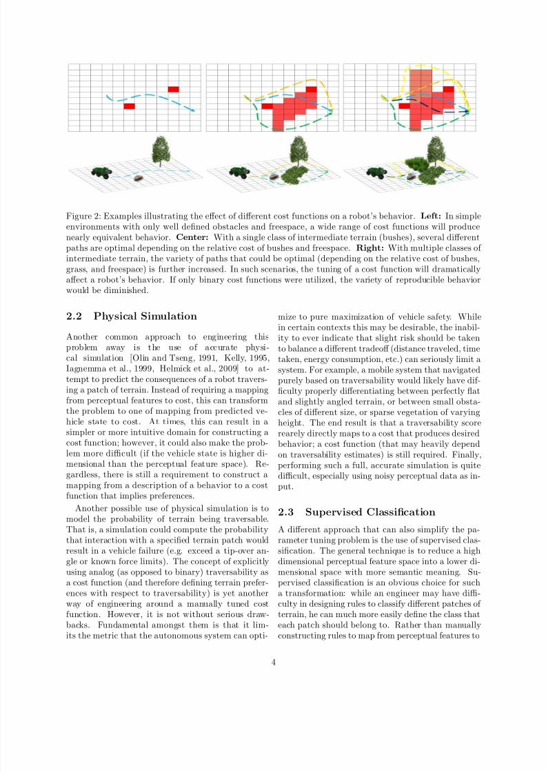
Figure 2: Examples illustrating the effect of different cost functions on a robot’s behavior. Left: In simpleenvironments with only well defined obstacles and freespace, a wide range of cost functions will producenearly equivalent behavior. Center: With a single class of intermediate terrain (bushes), several differentpaths are optimal depending on the relative cost of bushes and freespace. Right: With multiple classes of intermediate terrain, the variety of paths that could be optimal (depending on the relative cost of bushes,

grass, and freespace) is further increased. In such scenarios, the tuning of a cost function will dramaticallyaffect a robot’s behavior. If only binary cost functions were utilized, the variety of reproducible behaviorwould be diminished.

2.2 Physical Simulation

Another common approach to engineering thisproblem away is the use of accurate physi-cal simulation [Olin and Tseng, 1991, Kelly, 1995,Iagnemma et al., 1999, Helmick et al., 2009] to at-tempt to predict the consequences of a robot travers-ing a patch of terrain. Instead of requiring a mappingfrom perceptual features to cost, this can transformthe problem to one of mapping from predicted ve-hicle state to cost. At times, this can result in asimpler or more intuitive domain for constructing acost function; however, it could also make the prob-lem more difficult (if the vehicle state is higher di-mensional than the perceptual feature space). Re-gardless, there is still a requirement to construct amapping from a description of a behavior to a costfunction that implies preferences.

Another possible use of physical simulation is tomodel the probability of terrain being traversable.That is, a simulation could compute the probability

that interaction with a specified terrain patch wouldresult in a vehicle failure (e.g. exceed a tip-over an-gle or known force limits). The concept of explicitlyusing analog (as opposed to binary) traversability asa cost function (and therefore defining terrain prefer-ences with respect to traversability) is yet anotherway of engineering around a manually tuned costfunction. However, it is not without serious draw-backs. Fundamental amongst them is that it lim-its the metric that the autonomous system can opti-

mize to pure maximization of vehicle safety. Whilein certain contexts this may be desirable, the inabil-ity to ever indicate that slight risk should be takento balance a different tradeoff (distance traveled, timetaken, energy consumption, etc.) can seriously limit asystem. For example, a mobile system that navigatedpurely based on traversability would likely have dif-ficulty properly differentiating between perfectly flat

and slightly angled terrain, or between small obsta-cles of different size, or sparse vegetation of varyingheight. The end result is that a traversability scorerearely directly maps to a cost that produces desiredbehavior; a cost function (that may heavily dependon traversability estimates) is still required. Finally,performing such a full, accurate simulation is quitedifficult, especially using noisy perceptual data as in-put.

2.3 Supervised Classification

A different approach that can also simplify the pa-

rameter tuning problem is the use of supervised clas-sification. The general technique is to reduce a highdimensional perceptual feature space into a lower di-mensional space with more semantic meaning. Su-pervised classification is an obvious choice for sucha transformation: while an engineer may have diffi-culty in designing rules to classify different patches of terrain, he can much more easily define the class thateach patch should belong to. Rather than manuallyconstructing rules to map from perceptual features to

4



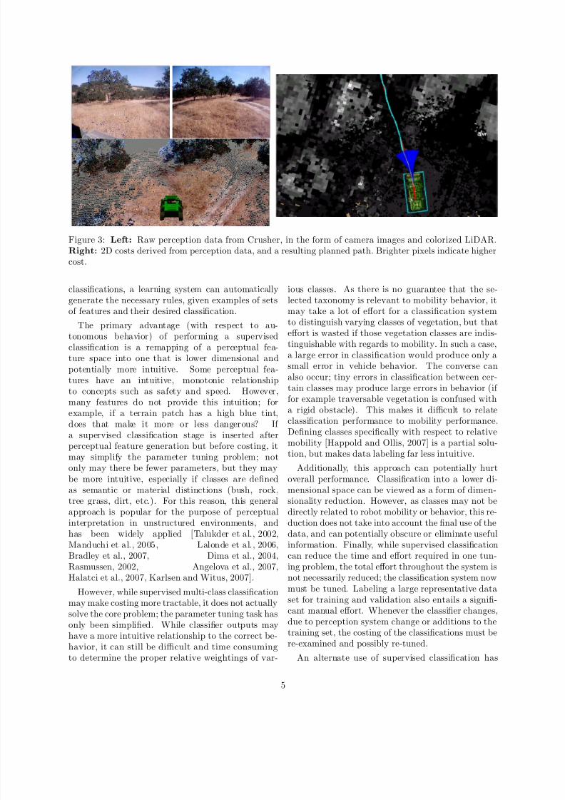
Figure 3: Left: Raw perception data from Crusher, in the form of camera images and colorized LiDAR.Right: 2D costs derived from perception data, and a resulting planned path. Brighter pixels indicate highercost.

classifications, a learning system can automaticallygenerate the necessary rules, given examples of setsof features and their desired classification.

The primary advantage (with respect to au-tonomous behavior) of performing a supervisedclassification is a remapping of a perceptual fea-ture space into one that is lower dimensional andpotentially more intuitive. Some perceptual fea-tures have an intuitive, monotonic relationshipto concepts such as safety and speed. However,many features do not provide this intuition; forexample, if a terrain patch has a high blue tint,does that make it more or less dangerous? If a supervised classification stage is inserted afterperceptual feature generation but before costing, itmay simplify the parameter tuning problem; notonly may there be fewer parameters, but they maybe more intuitive, especially if classes are definedas semantic or material distinctions (bush, rock,tree grass, dirt, etc.). For this reason, this generalapproach is popular for the purpose of perceptualinterpretation in unstructured environments, andhas been widely applied [Talukder et al., 2002,Manduchi et al., 2005, Lalonde et al., 2006,

Bradley et al., 2007, Dima et al., 2004,Rasmussen, 2002, Angelova et al., 2007,Halatci et al., 2007, Karlsen and Witus, 2007].

However, while supervised multi-class classificationmay make costing more tractable, it does not actuallysolve the core problem; the parameter tuning task hasonly been simplified. While classifier outputs mayhave a more intuitive relationship to the correct be-havior, it can still be difficult and time consumingto determine the proper relative weightings of var-

ious classes. As there is no guarantee that the se-lected taxonomy is relevant to mobility behavior, itmay take a lot of effort for a classification systemto distinguish varying classes of vegetation, but thateffort is wasted if those vegetation classes are indis-tinguishable with regards to mobility. In such a case,a large error in classification would produce only asmall error in vehicle behavior. The converse canalso occur; tiny errors in classification between cer-tain classes may produce large errors in behavior (if for example traversable vegetation is confused witha rigid obstacle). This makes it difficult to relate

classification performance to mobility performance.Defining classes specifically with respect to relativemobility [Happold and Ollis, 2007] is a partial solu-tion, but makes data labeling far less intuitive.

Additionally, this approach can potentially hurtoverall performance. Classification into a lower di-mensional space can be viewed as a form of dimen-sionality reduction. However, as classes may not bedirectly related to robot mobility or behavior, this re-duction does not take into account the final use of thedata, and can potentially obscure or eliminate usefulinformation. Finally, while supervised classification

can reduce the time and effort required in one tun-ing problem, the total effort throughout the system isnot necessarily reduced; the classification system nowmust be tuned. Labeling a large representative dataset for training and validation also entails a signifi-cant manual effort. Whenever the classifier changes,due to perception system change or additions to thetraining set, the costing of the classifications must bere-examined and possibly re-tuned.

An alternate use of supervised classification has

5



been to treat the task as a specific two class prob-lem: classifying terrain as either traversable ornon-traversable. Labels can be gathered either of-fline [Seraji and Howard, 2002, Howard et al., 2007]or online [Thrun et al., 2006, Sun et al., 2007] by ob-serving where an expert drives a robot; nearby

terrain that is not traversed is treated as havingbeen labeled non-traversable in a noisy manner1.[Ollis et al., 2007] involves similar data collection,but only for labeling of traversable terrain; explicitexamples of non-traversable regions are not required.The issues with this approach are twofold. First, thelabeling is likely to be very noisy, especially if exam-ples of non-traversable terrain are obtained by usingterrain located near traversable examples. More im-portantly, just as with physical simulation a probabil-ity of traversability, even if accurate, rarely directlymaps to the correct behavior.

2.4 Self-Supervised Learning from

Experience

In contrast with learning approaches that require ex-plicit supervision from an (usually human) expert,self-supervised approaches require no expert interac-tion. Instead, a robot uses its own interactions withthe world to slowly learn how to interpret what it per-ceives; the robot learns and adapts from experience.As opposed to requiring outside supervision and in-struction, the robot can learn from its own mistakes.This allows robots equipped with self-supervision to

adapt to novel environments or scenarios with littleto no human intervention, and is a powerful tool forachieving both robustness and reusability. Unsurpris-ingly, online self-supervised approaches to learninghave gained increasing popularity in recent years.

Approaches for self-supervised online learning canbe divided into two distinct classes. The first isnear-to-far learning that learns how to interpreta far-range, lower resolution sensor using a nearrange, higher-resolution sensor. Near-to-far learningis achieved by recalling how specific patches of terrainwere perceived by a far range sensor, and then laterobserving them with a near-range sensor. This pro-

vides a correspondence between the output of the twosensing modalities, and provides the necessary datato learn a mapping. Examples of such approaches in-clude learning to interpret monocular vision systemsfrom shorter range LiDAR [Dahlkamp et al., 2006]or stereo [Hadsell et al., 2009] range data, learn-

1This approach is fundamentally different from standardimitation learning in that demonstration is used purely as adata labeling technique; offline hand labeling could be usedwith similar results

Figure 4: An example of near-to-far learning from[Sofman et al., 2006]. In this example, as a robotdrives through an environment (left to right) it usesits short range sensors to train the interpretation of a far range sensor (in this case the satellite image atleft)

ing to map near range traversability estimatesto far range estimates [Bajracharya et al., 2008,Procopio et al., 2007], and learning to map full costfunctions from near to far [Sofman et al., 2006] (Fig-ure 4). However, near-to-far learning still requiresa (preexisting) correct interpretation of near-rangesensors. In fact, this near-range interpretation is in-creased in importance, since it is being used as aground truth signal for learning.

The other distinct class of self-supervised learningis learning from proprioception, also called learningfrom underfoot. As opposed to near-to-far learning,the ground truth signal comes not from a higherresolution exteroceptive sensor, but from propri-oceptive sensors. Aside from this distinction, themethodology is quite similar: as the robot drives

over a patch of terrain, it recalls how that terrainappeared in its near-range sensors just momentsago. This sets up a correspondence between howterrain appears, and how the robot interacts withit. These correspondences can be used to learnto model the robot’s interactions with terrainby predicting various terramechanical properties,such as roughness [Stavens and Thrun, 2006],vehicle slip [Angelova et al., 2007], soil cohesion[Iagnemma et al., 2004], or vegetation height

6



[Wellington et al., 2006]. Predictions can then beeither be used directly to determine robot behav-ior (i.e. as input into a cost function), or usedto improve the accuracy of a physical simulation[Helmick et al., 2009]. While these approaches cer-tainly provide useful information that can drastically

improve a robot’s robustness and adaptation, they donot directly address the general problem of mappingfrom features of terrain to terrain preferences.

Another approach to learning from proprioceptionis to attempt to directly learn traversability by ob-serving what terrain a robot can and can not success-fully traverse [Shneier et al., 2008, Kim et al., 2006].However, this approach has the same drawbacksas previously described techniques based on puretraversability. That is, it ignores the possibility of rel-ative preferences amongst equally traversable patchesof terrain. This issue also applies to other singlemetric learning from proprioception; for example, a

robot that learns to estimate its own speed over dif-ferent terrains would never be able to differentiatebetween terrains on which maximum speed is possi-ble but different mobility risk is encountered. Moreimportantly, this online approach to labeling terrainas non-traversable requires explicit interaction withnon-traversable terrain (e.g. the robot must driveinto an obstacle to learn that it is an obstacle). Notonly is this dangerous, it also results in a poten-tially difficult blame assignment problem (determin-ing which patch or patches of terrain were responsiblefor a failure).

2.5 Learning From Expert Demon-

stration

Given the difficulty in manually engineering acoupling between perception and planning systems,an alternative solution is to avoid this problemaltogether by learning to directly map perception toactions. This can be accomplished through learn-ing from demonstration, also known as imitationlearning. A key principle of imitation learning isthat while it may be very difficult to quantify whya certain behavior is desirable, the actual correct

behavior is usually known by a human expert.Therefore, rather than having a human experttune a system to achieve desired behavior, theexpert can demonstrate desired behavior and therobot can tune itself to match the demonstration.Learning from demonstration has a long historywith mobile robotics, starting with the ALVINNsystem [Pomerleau, 1989] and continuing throughmore recent applications [LeCun et al., 2006,Howard et al., 2005, Hamner et al., 2006].

These approaches to learning from demonstrationall fall into the category of action prediction: giventhe state of the world, or features of the state of theworld, they attempt to predict the action that the hu-man demonstrator would have selected. The funda-mental problem with pure action prediction is that it

is a purely reactive approach to planning. There is noattempt to model or reason about the consequences of a chosen action. Therefore, all relevant informationmust be encoded in the current state or features of the state. For certain scenarios this is feasible; pathtrackers are a classic example. However, in generalthe use of purely reactive systems is incredibly diffi-cult for planning long range, goal directed behaviorthrough complex unstructured environments.

An alternative to action prediction finds its roots inthe idea of Inverse Optimal Control [Kalman, 1964].While optimal control seeks a trajectory through astate space that optimizes some known metric, in-

verse optimal control seeks a metric such that aknown trajectory through a state space is optimal un-der said metric. Within mobile robotics, the parallelwould be to learn a cost function such that a robot’splanning system will reproduce expert2 demonstratedbehavior. Such an approach automates the hand con-struction and tuning of cost functions that is preva-lent in actual deployments. Not only does automat-ing this procedure result in large reduction in designeffort, it can potentially produce a better coupling;automatic optimization need not be nearly as con-cerned with diminishing returns, and can continueuntil convergence. Further, an automated approach

can take advantage of standard cross validation tech-niques to ensure that a learned coupling is robust andwill generalize well. Finally, if collection of expertdemonstration includes raw sensor data, changes tosensor processing within a perception system do notresult in additional human effort with respect to acost function; existing demonstrations can simply bereprocessed and coupling relearned.

Inverse Reinforcement Learning [Ng and Russell, 2000] was the first applicationof this idea to the framework of Markov DecisionProcesses commonly used for motion planning in

mobile robotics. This framework was later modifiedinto a new approach known as Apprenticeship Learn-ing [Abbeel and Ng, 2004]. Apprenticeship learningresulted in an algorithm that produced linear costfunctions such that any planned behavior would havethe same cost as demonstrated behavior (betweenequivalent start and end conditions); however there

2This expert need no longer be a full system expert, butrather only needs to have the necessary intuition to understandhow the robot should drive

7



was no mechanism for explicitly matching expertbehavior. Additionally, the final solution was astochastic mixture of multiple policies. The Maxi-mum Margin Planning (MMP) [Ratliff et al., 2006]framework addressed these problems by producinga single deterministic solution while also ensuring

an upper bound on the mismatch between demon-strated and planned behavior. More recent work hasextended the MMP framework to non-linear costfunctions [Ratliff et al., 2009, Silver et al., 2008], andwas applied to Crusher for the task of learning a costfunction to interpret both static and dynamic percep-tual data [Silver et al., 2009a, Silver et al., 2009b].

3 Learning to Interpret Per-

ceptual Data from Expert

Demonstration

The MMP framework treats learning from demon-stration as a constrained optimization problem. Indecision theory, a utility function is defined as a rela-tive ordering over all possible options. Since mostmobile robotic systems encounter an infinite num-ber of possible plans, such an explicit ordering is notpossible. Instead, plans are scored by a cost func-tion, and cost defines the ordering. However, thiscore idea of an ordering of preferences remains use-ful. If an expert can concretely define a relative or-

dering over even a small subset of possible plans, thisordering becomes a constraint on the cost function:the costs assigned to each possible plan must matchthe relative ordering. The more information on rela-tive preferences an expert provides, the more the costfunction is constrained.

This section first derives the basic MMP algo-rithm for learning a linear cost function to repro-duce expert demonstration. Next the LEARCH al-gorithm (LEArning to seaRCH) [Ratliff et al., 2009,Silver et al., 2008] is presented for extending this ap-proach to non-linear cost functions. The MMP frame-

work and associated algorithms are defined over gen-eral Markov Decision Processes. However, withoutloss of generality, this derivation is restricted to deter-ministic MDPs with a set of absorbing states; that is,goal directed path or motion planners. This changeis purely for notational simplification, as most mo-bile robotic systems use planners of this form. Ad-ditionally, only cost functions defined over states areconsidered, as opposed to full state-action pairs (seeSection 6).

3.1 Maximum Margin Planning with

Linear Cost Functions

Consider a state space S through which a planneroperates (e.g. S = R

2). A feature space F is de-fined over S . That is, for every x ∈ S , there exists

a corresponding feature vector F x ∈ F . F x can beconsidered as the raw output of a perception systemat state x3. For the output of a perception system tobe used by a planner, it must be mapped to a scalarcost value; Therefore, C is defined as a cost function,C : F → R

+. The cost of a state x is C (F x). Forthe moment, only linear cost functions of the formC (F ) = wT F are considered; the weight vector wcompletely defines the cost function. Finally, a pathP is defined as a sequence of states in S that leadfrom a start s to a goal g. The cost of an entirepath is simply defined as the sum of the costs of allstates along the path, or alternatively the cost of the

cumulative feature counts

C (P ) =x∈P

C (F x) =x∈P

wT F x = wT x∈P

F x (1)

Now consider an example path P e from a start statese to a goal state ge. If this example path is pro-vided via expert demonstration, then its is reasonableto consider applying inverse optimal control; that is,seeking to find a cost function C such that P e is theoptimal path from se to ge. While a single exampledemonstration does not imply a single cost function,

it does constrain the space of cost functions C: onlycost functions that consider P e the optimal path areacceptable. For now, it is assumed that all P e are atleast near optimal under at least one C ∈ C; Section4.2 will relax this assumption.

If a regularization term is also added to encouragesimple solutions, then the task of finding an accept-able cost function from an example can be phrasedas the following constrained optimization problem:

minimize O(w) = ||w||2 (2)

subject to the constraints

x∈P

(wT F x)≥

x∈P e

(wT F x)

∀P s.t. P = P e, s = se, g = ge

Unfortunately, this optimization has a trivial so-lution: w = 0. This issue can be addressed by in-cluding a margin in each constraint. The size of the

3For now it is assumed that the assignment of a featurevector to a state is static; the extension to dynamic assignmentis addressed in Section 4.1

8



margin is dependent on the similarity between paths;the example only needs to be slightly lower cost thana very similar path, but should be much lower costthan a very different path. Similarity between P e andan arbitrary path P is encoded by a loss functionL(P e, P ), or alternatively Le(P )4. The definition of

the loss function is somewhat application dependant;the simplest form would be to simply consider howmany states the two paths share (a Hamming loss).The effect of the scale of the margin is removed bythe regularization term. The constrained optimiza-tion can now be rewritten as


subject to the constraints

x∈P

(wT F x − Le(x)) ≥x∈P e

(wT F x)

∀P s.t. P = P e, s = se, g = ge

Le(x) =

1 if x ∈ P e0 otherwise

Depending on the state space, and the distancefrom se to ge, there are likely to be an infeasible (andpossibly infinite) number of constraints; one for eachalternate path to the demonstrated example. How-ever, it is not necessary to enforce every constraint.For any candidate cost function, there is a minimum

cost path between any two waypoints, P ∗. It is onlynecessary to enforce the constraint for P ∗, as once itis satisfied by definition all other constraints will besatisfied. With this single constraint, (3) becomes


subject to the constraintx∈P ∗

(wT F x − Le(x)) ≥

x∈P e

(wT F x)

P ∗ = arg minP

x∈P

(wT F x − Le(x))

It may not always be possible to exactly meetthis constraint (the margin may make it impossible).Therefore, a slack term ζ is added to allow for thispossibility.

4As a path is considered just a sequence of states, the lossfunction can be defined either over a full path or over a singlestate.

minimize O(w) = λ||w||2 + ζ (5)

subject to the constraint

x∈P ∗

(wT F x − Le(x)) −x∈P e

(wT F x) + ζ ≥ 0

The slack term ζ accounts for the error in meet-ing the constraint, while λ balances the tradeoff inthe objective between regularization and meeting theconstraint. However, the slack variable will alwaysbe tight; that is ζ will always be exactly equal to thedifference in path costs. Therefore, ζ can be replacedin the objective by the constraint, resulting in thefollowing (unconstrained) optimization problem

minimize O(w) = λ||w||2 + (6)

x∈P e

(wT

F x) − x∈P ∗

(wT

F x − Le(x))

or alternatively

minimize O(w) = λ||w||2 + (7)

x∈P e

(wT F x) − minP

x∈P

(wT F x − Le(x))

The final optimization seeks to minimize the dif-ference in cost between the example path P e and the(loss augmented) optimal path P ∗, subject to reg-

ularization. O(w) is convex, but non-differentiable;therefore, instead of gradient descent, it can be min-imized using the sub-gradient method with learningrate η. The sub-gradient of O with respect to w is

O = 2λw +

x∈P e

F x −

x∈P ∗

F x (8)

Intuitively, (8) says that the direction that willmost minimize the objective function is found bycomparing feature counts. If more of a certain fea-ture is encountered on the example path than thecurrent minimum cost path P ∗, the weight on that

feature (and therefore the cost) should be decreased.Likewise, if less of a feature is encountered on theexample path than on P ∗, the weight should be in-creased. Although the margin does not appear in thefinal sub-gradient, it does affect the computation of P ∗. The final linear MMP algorithm consists of iter-atively computing feature counts and then updatingthe cost function until convergence. However, one fi-nal caveat is to ensure that only cost functions thatmap to R

+ are considered (a requirement of most

9



Algorithm 1: The linear MMP algorithm

Inputs : Example Paths P 1e , P 2e ,...,P ne ,Feature Map F

w0 = 0;for j = 1...K do

M= buildCostmap(wj−1,

F );

F e = F ∗ = 0;foreach P ie do

P i∗ = planLossAugPath(start(P ie),goal(P ie),M);

foreach x ∈ P ie doF e+ = F e + F x;

foreach x ∈ P i∗ doF ∗ = F ∗ + F x;

wj = wn−1 + ηi[F ∗ − F e − λwj−1];enforcePositivityConstraint (wj ,F );

return wK

motion and path planners). This is achieved by iden-tifying F such that wT F ≤ 0, and projecting w backinto the space of allowable cost functions.

The MMP framework easily supports the use of multiple example paths. Each example implies itsown constraints as in (4), its own objective as in (7),and its own sub-gradient as in (8). Updating the costweights can take place either on a per example basis,or the feature counts can be computed in a batchwith a single update. The latter is computationallypreferable, as it may result in fewer cost function eval-uations, and projections back into the space of allow-able cost functions. The final linear MMP algorithmis presented in Algorithm 1.

3.2 MMP with Non-Linear Cost

Functions

The derivation to this point has assumed that thespace of possible cost functions C consists of all func-tions of the form C (F ) = wT F . Extension to other,more descriptive spaces of cost functions is possibleby considering (7) for any cost function C

minimize O[C ] = λReg(C ) (9)

+

x∈P e

C (F x) − minP

x∈P

(C (F x) − Le(x))

O[C ] is now an objective functional over a cost func-tion, and Reg represents a regularization functional.We can now consider the sub-gradient in the space of

cost functions

OF [C ] = λRegF [C ]+

x∈P e

δF (F x) −

x∈P ∗

δF (F x)

(10)

P ∗ = arg minP

x∈P

(C (F x) − Le(x))

where δ is the Dirac delta at the point of evaluation.Simply speaking, the functional gradient is positiveat values of F corresponding to states in the examplepath, and negative at values of F corresponding tostates in the current planned path. If the paths bothcontain a state corresponding to F , their contribu-tions cancel.

Applying gradient descent directly in this spacewould result in an extreme form of overfitting; es-sentially, it would involve raising or lowering the costassociated with specific values of F encountered oneither path, and would therefore produce no general-

ization whatsoever. Instead, a different space of costfunctions is considered

C ={C | C =

i

ηiRi(F ), Ri ∈ R, ηi ∈ R} (11)

R ={R | R : F → R ∧ Reg(R) < ν }C is now defined as the space of weighted sums of functions Ri ∈ R, where R is a space of functions of limited complexity that map from the feature spaceto a scalar. Choices of R include linear functions,parametric functions, neural networks, decision trees,etc. As in gradient boosting [Mason et al., 2000], this

space represents a limited set of ‘directions’ for whicha small step can be taken; the choice of the directionset in turn controls the complexity of C.

With this new definition, a gradient descent updatetakes the form of projecting the functional gradient5

onto the direction set by finding the element R∗ ∈ Rthat maximizes the inner product −OF [C ], R∗.The maximization of the inner product between thefunctional gradient and the hypothesis space can beunderstood as a learning problem:

R∗ = arg maxR

−OF [C ], R

= arg maxR

x∈P e∩P ∗

−OF [C ]R(F x)

= arg maxR

x∈P e∩P ∗

αxyxR(F x) (12)

αx = | OF x[C ]| yx = −sgn(OF x [C ])

In this form, it can be seen that finding the projectionof the functional gradient involves solving a weighted

5For the moment, the regularization term is ignored.

10



classification problem; the element of R that bestdiscriminates between features vectors for which thecost should be raised or lowered maximizes the in-ner product. Alternatively, defining R as a class of regressors adds an additional regularization to eachindividual R∗ [Ratliff et al., 2009]. Intuitively, the re-

gression targets yx are positive in regions of the fea-ture space that the planned path visits more than theexample path (indicating a desire to raise the cost),and negative in regions that the example path visitsmore than the planned path. Each regression targetis weighted by a factor αx based on the magnitude of the functional gradient.

In comparison to the linear MMP formulation, thisapproach can be understood as trying to minimize theerror in visitation counts instead of feature counts.For a given feature vector F and path P , the visita-tion count U is the cumulative count of the numberof states x

∈P such that F x = F . The visitation

counts can be split into positive and negative com-ponents, corresponding to the current planned andexample paths. Formally

U +(F ) =

x∈P ∗

δF (F x)

U −(F ) =

x∈P e

δF (F x)

U (F ) = U + − U − =

x∈P ∗

δF (F x) −

x∈P e

δF (F x)

(13)

Comparing this formulation to (10) demonstratesthat the planned visitation counts minus the examplevisitation counts equals the negative functional gra-dient (ignoring regularization). This allows for thecomputation of regression targets and weights purelyas a function of the visitation counts, providing astraight forward implementation (Algorithm 2) mak-ing use of off the shelf regression approaches (repre-sented by Rj ).

A final addition to this algorithm involves a slightlydifferent approach to optimization. Gradient descentcan be understood as encouraging functions that are

’small’ in the l2 norm; by controlling the learningrate η and the number of epochs, it is possible toconstrain the complexity of the learned cost function.However, instead we can consider exponentiated func-tional gradient descent , which is a generalization of exponentiated gradient to functional gradient descent[Ratliff et al., 2009]. Exponentiated functional gradi-ent descent encourages functions that are ‘sparse’ inthe sense of having many small values and a few po-tentially large values. This change results in C being

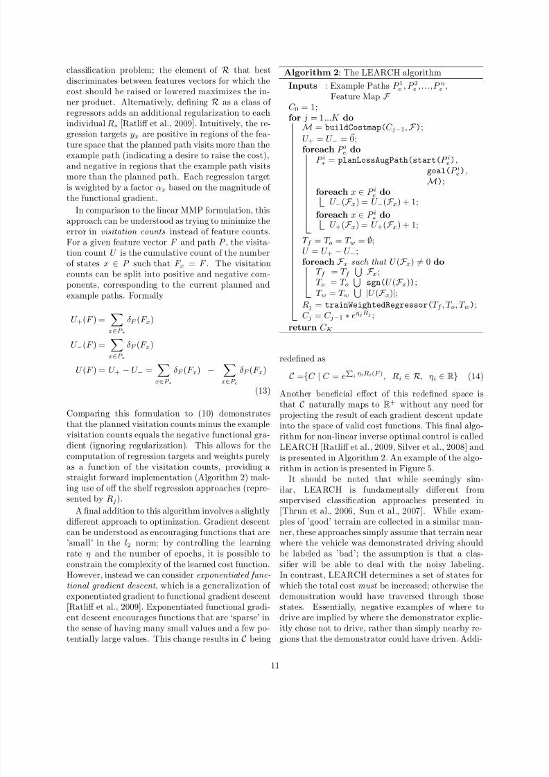
Algorithm 2: The LEARCH algorithm

Inputs : Example Paths P 1e , P 2e ,...,P ne ,Feature Map F

C 0 = 1;for j = 1...K do

M= buildCostmap(C j−1,

F );

U + = U − = 0;foreach P ie do

P i∗ = planLossAugPath(start(P ie),goal(P ie),M);

foreach x ∈ P ie doU −(F x) = U −(F x) + 1;

foreach x ∈ P i∗ doU +(F x) = U +(F x) + 1;

T f = T o = T w = ∅;U = U + − U −;foreach

F x such that U (

F x)

= 0 do

T f = T f F x;

T o = T o

sgn(U (F x));T w = T w

|U (F x)|;Rj = trainWeightedRegressor(T f , T o, T w);C j = C j−1 ∗ eηjRj ;

return C K

redefined as

C ={C | C = eP

iηiRi(F ), Ri ∈ R, ηi ∈ R} (14)

Another beneficial effect of this redefined space is

that C naturally maps toR+

without any need forprojecting the result of each gradient descent updateinto the space of valid cost functions. This final algo-rithm for non-linear inverse optimal control is calledLEARCH [Ratliff et al., 2009, Silver et al., 2008] andis presented in Algorithm 2. An example of the algo-rithm in action is presented in Figure 5.

It should be noted that while seemingly sim-ilar, LEARCH is fundamentally different fromsupervised classification approaches presented in[Thrun et al., 2006, Sun et al., 2007]. While exam-ples of ’good’ terrain are collected in a similar man-ner, these approaches simply assume that terrain near

where the vehicle was demonstrated driving shouldbe labeled as ’bad’; the assumption is that a clas-sifier will be able to deal with the noisy labeling.In contrast, LEARCH determines a set of states forwhich the total cost must be increased; otherwise thedemonstration would have traversed through thosestates. Essentially, negative examples of where todrive are implied by where the demonstrator explic-itly chose not to drive, rather than simply nearby re-gions that the demonstrator could have driven. Addi-

11



Figure 5: An example of the LEARCH algorithm learning to interpret satellite imagery (Top) as costs(Bottom). Brighter pixels indicate higher cost. As the cost function evolves (left to right), the current plan(green) recreates more and more of the example plan (red). Quickbird imagery courtesy of Digital Globe,Inc. Images cover approximately 300 m X 250 m.

Figure 6: Generalization of the LEARCH algorithm. The cost function learned from the single example inFigure 5 generalizes over terrain never seen during training (shown at approximately 1/2 scale) resulting insimilar planner behavior. 3 sets of waypoints (Left) are shown along with the corresponding paths (Center)planned under the learned cost function (Right).

tionally, the terrain that the demonstration traversedis not explicitly considered as ’good’ terrain; ratherits costs are only lowered until the path is preferred(for specified waypoints); there could still be high costregions along it. This distinction allows LEARCH togeneralize well over areas for which is was not explic-itly trained (Figure 6).

4 Adaptation and Application

to Mobile Robotic Systems

4.1 Extension to Dynamic and Un-

known Environments

The previous derivation of MMP and LEARCH onlyconsidered the scenario where the mapping fromstates to features is static and fully known a pri-ori. Recent work [Silver et al., 2009b] has extendedthe LEARCH algorithm to the scenario where nei-ther of these assumptions holds, such as when fea-

tures are generated from a mobile robot’s perceptionsystem. The limited range inherent in onboard sens-ing implies a great deal of the environment may beunknown; for truly complex navigation tasks, the dis-tance between waypoints is generally at least one ortwo orders of magnitude larger than the sensor range.Further, changing range and point of view from envi-ronmental structures means that even once an objectis within range, its perceptual features are continu-ally changing. Finally, there are the actual dynamicsof the environment: objects may move, lighting andweather conditions can change, etc.

Since onboard perceptual inputs are not static, arobot’s current plan must be continually recomputed.The original MMP constraint must be altered in thesame way: rather than enforcing the optimality of the entire example behavior once, the optimality of allexample behavior must be continually enforced as thecurrent plan is recomputed. Formally, we add a timeindex t to account for dynamics. F tx represents theperceptual features of state x at time t. P te represents

12



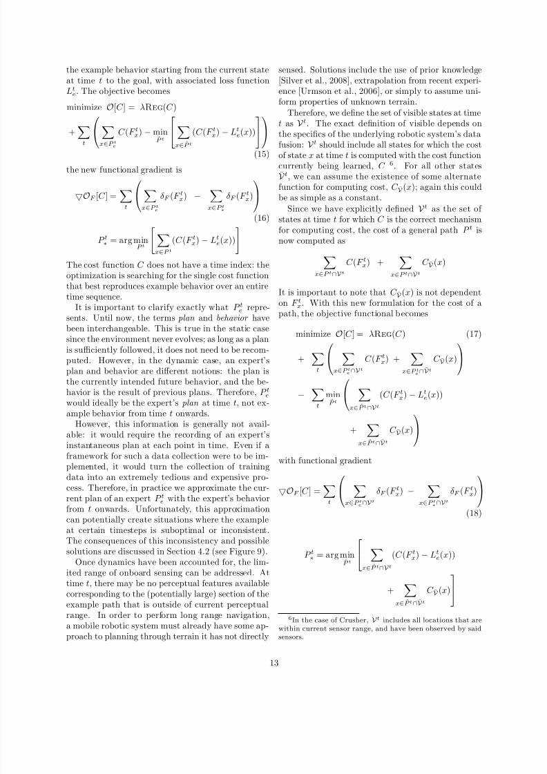
the example behavior starting from the current stateat time t to the goal, with associated loss functionLt

e. The objective becomes

minimize O[C ] = λReg(C )

+

t

x∈P te

C (F t

x) − minP t

x∈P t(C (F

t

x) − Lt

e(x))(15)

the new functional gradient is

OF [C ] =

t

x∈P te

δF (F tx) −

x∈P t∗

δF (F tx)

(16)

P t∗ = arg minP t

x∈P t

(C (F tx) − Lte(x))

The cost function C does not have a time index: theoptimization is searching for the single cost functionthat best reproduces example behavior over an entiretime sequence.

It is important to clarify exactly what P te repre-sents. Until now, the terms plan and behavior havebeen interchangeable. This is true in the static casesince the environment never evolves; as long as a planis sufficiently followed, it does not need to be recom-puted. However, in the dynamic case, an expert’splan and behavior are different notions: the plan isthe currently intended future behavior, and the be-havior is the result of previous plans. Therefore, P te

would ideally be the expert’s plan at time t, not ex-ample behavior from time t onwards.However, this information is generally not avail-

able: it would require the recording of an expert’sinstantaneous plan at each point in time. Even if aframework for such a data collection were to be im-plemented, it would turn the collection of trainingdata into an extremely tedious and expensive pro-cess. Therefore, in practice we approximate the cur-rent plan of an expert P te with the expert’s behaviorfrom t onwards. Unfortunately, this approximationcan potentially create situations where the exampleat certain timesteps is suboptimal or inconsistent.

The consequences of this inconsistency and possiblesolutions are discussed in Section 4.2 (see Figure 9).

Once dynamics have been accounted for, the lim-ited range of onboard sensing can be addressed. Attime t, there may be no perceptual features availablecorresponding to the (potentially large) section of theexample path that is outside of current perceptualrange. In order to perform long range navigation,a mobile robotic system must already have some ap-proach to planning through terrain it has not directly

sensed. Solutions include the use of prior knowledge[Silver et al., 2008], extrapolation from recent experi-ence [Urmson et al., 2006], or simply to assume uni-form properties of unknown terrain.

Therefore, we define the set of visible states at timet as V t. The exact definition of visible depends on

the specifics of the underlying robotic system’s datafusion: V t should include all states for which the costof state x at time t is computed with the cost functioncurrently being learned, C 6. For all other statesV t, we can assume the existence of some alternatefunction for computing cost, C V (x); again this couldbe as simple as a constant.

Since we have explicitly defined V t as the set of states at time t for which C is the correct mechanismfor computing cost, the cost of a general path P t isnow computed as

x∈P t∩V t

C (F tx) + x∈P t∩V t

C V (x)

It is important to note that C V (x) is not dependenton F tx. With this new formulation for the cost of apath, the objective functional becomes


+

t

x∈P te∩V t

C (F tx) +

x∈P te∩V t

C V (x)

− t

minP t

x∈P t∩V t


+

x∈P t∩V t

C V (x)

with functional gradient

OF [C ] =

t

x∈P te∩V t

δF (F tx) −

x∈P t∗∩V t

δF (F tx)

(18)

P t∗ = arg minP t

x∈P t∩V t


+

x∈P t∩V t

C V (x)

6In the case of Crusher, V t includes all locations that arewithin current sensor range, and have been observed by saidsensors.

13



since the gradient is computed with respect to C , itis only nonzero for visible states; the C V (x) termsdisappear. However, C V still factors into the plannedbehavior, and therefore does affect the learned com-ponent of the cost function. Just as LEARCH learnsC to recreate desired behavior when using a specific

planner, it learns C to recreate behavior when us-ing a specific C V . However, if the example behavioris inconsistent with C V , it will be more difficult forthe planned behavior to match the example. Suchan inconsistency could occur if the expert has differ-ent prior knowledge than the robot, or interprets thesame knowledge differently. Inconsistency can alsooccur due to the previously discussed mismatch be-tween expert plans and expert behavior. A solutionto this problem is discussed in Section 4.2.

The projection of the functional gradient onto thehypothesis space becomes

R∗ = arg maxR

t

x∈(P e∪P ∗)∩V t

αtxyt

xR(F tx) (19)

Contrasting the final form for R∗ with that of (12) helps to summarize the changes that result inthe LEARCH algorithm for dynamic environments.Specifically, a single expert demonstration from startto goal is discretized by time, with each timestep serv-ing as an example of what behavior to plan given alldata to that point in time. For each of these dis-cretized examples, only visitation counts in visiblestates are used. The resulting algorithm is presented

as Algorithm 3.A final detail for a LEARCH implementation is thesource of the input perceptual features. Rather thancomputing and logging these features online, it is use-ful to record all raw sensor data, and then to computethe features by simulating perception offline. Thisallows existing expert demonstration to be reused if new feature extractors are added, or existing onesmodified; perception is simply re-simulated to pro-duce the new inputs. In this way, learning a costfunction when the perception system is modified re-quires no additional expert interaction.

4.2 Imperfect and InconsistentDemonstration

The MMP framework implicitly assumes that one ormore cost functions exist under which demonstratedbehavior is near optimal. Generally this is not thecase, as there will always be noise in human demon-stration. Further, multiple examples possibly col-lected from different environments and different ex-perts may be inconsistent with each other (due to

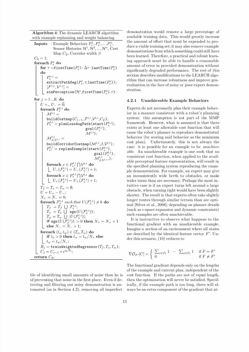
Algorithm 3: The dynamic LEARCH algorithm

Inputs : Example Behaviors P 1e , P 2e ,...,P ne ,Sensor Histories H1, H2,..., Hn, CostMap C V

C 0 = 1;foreach P ie do

for τ =firstTime(P ie): ∆τ :lastTime(P ie)do

P τ,ie =

extractPathSeg(P ie , τ,lastTime(P ie));[F τ,i, V τ,i] =simPerception(Hi,firstTime(P ie),τ );

for j = 1...K do

U += U − = 0;foreach P t,i

e do

Mt,i =buildCostmap(C i−1, F t,i,V t,i,C V );P t,i∗ = planLossAugPath(start(P t,i

e ),

goal(P t,ie ),Mt,i);foreach x ∈ P t,i

e

V t,i do

U −(F t,ix ) = U −(F t,i

x ) + 1;

foreach x ∈ P t,i∗

V t,i do

U +(F t,ix ) = U +(F t,i

x ) + 1;

T f = T o = T w = ∅;U = U + − U −;foreach F t,i

x such that U (F t,ix ) = 0 do

T f = T f

F t,ix ;

T o = T o

sgn(U (F t,i

x ));T w = T w |

U (

F t,ix )

|;

Rj = trainWeightedRegressor(T f , T o, T w);C j = C j−1 ∗ eηjRj ;

return C K

inconsistency in human behavior, a different conceptof what is desirable, or an incomplete perceptual de-scription of the environment by the robot.) Finally,sometimes experts are flat out wrong, and demon-strate behavior that is not even close to desirable.

While the MMP framework is robust to poor train-ing data, it does suffer degraded overall performance

and generalization, in the same way that supervisedclassification performance is degraded by noisy ormislabeled training data. Attempting to have an ex-pert sanitize the training input after initial demon-stration is disadvantageous for two reasons. First itcreates an additional need for human involvement,eliminating some of the time savings promised bythis approach. Second, it assumes that an expertcan detect all errors; while this may be true for ex-treme cases, a human expert may be no more capa-

14



Algorithm 4: The dynamic LEARCH algorithmwith example replanning and weight balancing

Inputs : Example Behaviors P 1e , P 2e ,...,P ne ,Sensor Histories H1, H2, ...,Hn, CostMap C V , Corridor width β

C 0 = 1;foreach P ie do

for τ =firstTime(P ie): ∆τ :lastTime(P ie)do

P τ,ie =

extractPathSeg(P ie , τ,lastTime(P ie));[F τ,i, V τ,i] =simPerception(Hi,firstTime(P ie),τ );

for j = 1...K do

U += U − = 0;foreach P t,i

e do

Mt,i =buildCostmap(C i−1,

F t,i,

V t,i,C V );

P t,i∗ = planLossAugPath(start(P t,ie ),goal(P t,i

e ),Mt,i);

Mt,i

β,V t,i=

buildCorridorCostmap(Mt,i,β ,V t,i);P t,i

e∗ = replanExample(start(P t,ie ),

goal(P t,ie ),

Mt,i

β,V t,i,);

foreach x ∈ P t,ie∗

V t,i do

U −(F t,ix ) = U −(F t,i

x ) + 1;

foreach x ∈ P t,i∗

V t,i do

U +(

F t,ix ) = U +(

F t,ix ) + 1;

T f = T o = T w = ∅;U = U + − U −;N + = N − = 0;foreach F t,i

x such that U (F t,ix ) = 0 do

T f = T f

F t,ix ;

T o = T o

sgn(U (F t,ix ));

T w = T w |U (F t,i

x )|;if sgn(U (F t,i

x )) > 0 then N + = N + + 1else N − = N − + 1;

foreach (to, tw) ∈ (T o, T w) doif to > 0 then tw = tw/N + else

tw = tw/N −;

Rj = trainWeightedRegressor(T f , T o, T w);C j = C j−1 ∗ eηjRj ;

return C K

ble of identifying small amounts of noise than he isof preventing that noise in the first place. Even if de-tecting and filtering out noisy demonstration is au-tomated (as in Section 4.2), removing all imperfect

demonstration would remove a large percentage of available training data. This would greatly increasethe amount of effort that must be expended to pro-duce a viable training set; it may also remove exampledemonstrations from which something could still havebeen learned. Therefore, a practical and robust learn-

ing approach must be able to handle a reasonableamount of error in provided demonstration withoutsignificantly degraded performance. The rest of thissection describes modifications to the LEARCH algo-rithm that can increase robustness and improve gen-eralization in the face of noisy or poor expert demon-stration.

4.2.1 Unachievable Example Behaviors

Experts do not necessarily plan their example behav-ior in a manner consistent with a robot’s planningsystem: this assumption is not part of the MMP

framework. However, what is assumed is that thereexists at least one allowable cost function that willcause the robot’s planner to reproduce demonstratedbehavior (by scoring said behavior as the minimumcost plan). Unfortunately, this is not always thecase: it is possible for an example to be unachiev-able. An unachievable example is one such that noconsistent cost function, when applied to the avail-able perceptual feature representation, will result inthe specified planning system reproducing the exam-ple demonstration. For example, an expert may givean inconsistently wide berth to obstacles, or makewider turns than are necessary. Perhaps the most in-

tuitive case is if an expert turns left around a largeobstacle, when turning right would have been slightlyshorter. The result is that experts often take slightlylonger routes through similar terrain than are opti-mal [Silver et al., 2008]; depending on planner details(such as c-space expansion and dynamic constraints)such examples are often unachievable.

It is instructive to observe what happens to thefunctional gradient with an unachievable example.Imagine a section of an environment where all statesare described by the identical feature vector F . Un-der this scenario, (10) reduces to

OF [C ] =

x∈P e

1 − x∈P ∗

1 if F = F

0 if F = F

The functional gradient depends only on the lengthsof the example and current plan, independent of thecost function. If the paths are not of equal length,then the optimization will never be satisfied. Specif-ically, if the example path is too long, there will al-ways be an extra component of the gradient that at-

15



(a) 3 Example Training Paths (b) Learned costmap with un-balanced weighting

(c) Learned costmap withbalanced weighting

(d) Ratio of the balanced tounbalanced costmaps

Figure 7: The red path is an unachievable example path, as it will be less expensive under any cost functionto cut more directly across the grass. With standard unbalanced weighting (b), the unachievable exampleforces down the cost of grass, and prevents the blue example from being achieved. Balanced weighting (c)prevents this bias, and the blue example is achieved. Overall, grass is approximately 12% higher cost withbalanced than unbalanced weighting (d)

tempts to lower costs at F . Intuitively, an unachiev-

able example implies that the cost of certain terrainshould be 0, as this would result in any path throughthat region being optimal. However, since costs areconstrained to R+, this will never be achieved. In-stead an unachievable example will have the effect of unnecessarily lowering costs over a large section of the feature space, and artificially reducing dynamicrange. Depending on the expressiveness of R, anunachievable example counteracts the constraints of other (achievable) paths, resulting in poorer perfor-mance and generalization (see Figure 7).

This negative effect can be avoided by performinga slightly different regression or classification when

projecting the gradient. Instead of minimizing theweighted error, the balanced weighted error is min-imized; that is, both positive and negative targetsmake an equal contribution. Formally, in (19) R∗ isreplaced with RB

∗ defined as

RB∗ = arg max

R

Xt

0@Xytx>0

αtxR(F tx)

N +−Xytx<0

αtxR(F tx)

N −

1A

N + =Xt

Xytx>0

αtx = |U +|1 N − =Xt

Xytx<0

αtx = |U −|1

(20)

In the extreme unachievable case described above,

RB

∗ will be zero everywhere; the optimization will besatisfied with the cost function as is. The effect of bal-ancing in the general case can be observed by rewrit-ing the regression operation in terms of the plannedand example visitation counts, and observing the cor-relation of their inputs.

R∗ = arg maxR, U + − U −RB∗ = arg maxR,

U +N +

− U −N −

Theorem 4.1. The regression targets of R∗ and

RB∗ are always correlated, except when the visitation counts between the example and planned path are per-

fectly correlated.

Proof.

U + − U −,U +N +

− U −N −

=U +, U +

N +− U +, U −

N ++

U −, U −N −

− U +, U −N −

=|U +|2

N ++

|U −|2N −

− (1

N ++

1

N −)U +, U − (21)

By the Cauchy-Schwarz inequality,U +, U −

is

bounded by |U +||U −|, and is only tight against thisbound when the visitation counts are perfectly corre-lated, which implies

U +, U − = |U +||U −| ⇐⇒ U − = κU +

=⇒ |U −| = κ|U +| , N − = κN +

for some scalar κ. By substitution

|U +|2N +

+|U −|2

N −− (

1

N ++

1

N −)U +, U −

≥ |U +|2N +

+|U −|2

N −− (

1

N ++

1

N −)|U +||U −|

= |U +|2N +

+ κ2|U +|2κN +

− ( 1N +

+ 1κN +

)κ|U +||U +|

=|U +|2

N ++

κ|U +|2N +

− |U +|2N +

− κ|U +|2N +

= 0

When U +, U − is not tight against the upper bound

U + − U −,U +N +

− U −N −

≥ 0

16



By (21) the similarity between inputs to the projec-tions is negatively correlated to the overlap of the pos-

itive and negative visitation counts. When there ex-ists clear differentiation between what features shouldhave their costs increased and decreased, the projec-tion inputs will be similar. As the example and cur-rent planned behaviors travel over increasingly sim-ilar terrain, the inputs being to diverge; the contri-bution of the balanced projection to the current costfunction will level out, while that of the unbalancedprojection will increase in the direction of the longerpath. Finally, in a fully unachievable case, the bal-anced projection will zero out, while the unbalancedwould drive the cost in the direction of the more dom-inant class. This effect is observed empirically in Sec-

tion 5. The implementation of this balancing is shownin Algorithm 4.

4.2.2 Noisy Demonstration: Replanning and

Corridor Constraints

A balanced regression can help to account for largescale sub-optimality in human demonstration. How-ever, sub-optimality can also occur at a smaller scale.It is unreasonable to ever expect a human to drive ordemonstrate the exact perfect path; it is often the

case that a plan that travels through neighboring ornearby states would be a slightly better example. Insome cases this example noise translates to noise inthe cost function; in more extreme cases it can signifi-cantly affect performance (Figure 8). What is neededis an approach that smoothes out small scale noisein expert demonstration, producing a better trainingexample.

Such a smoothed example can be derived fromexpert demonstration by redefining the MMP con-straint: instead of example behavior being inter-preted as the exact optimal behavior, it can be in-

terpreted as a behavior that is spatially near the op-timal path. The exact definition of ’close’ dependson the state space; the loss function will always pro-vide at least one possible metric. If the state spaceis Rn, then Euclidean distance is a natural metric.Therefore, rather than an example defining the exactoptimal path, it would define a corridor in which theoptimal path exists.

Redefining the original MMP constraint in (4) inthis way yields

minimize O[C ] = λReg[C ] (22)

subject to the constraint

x∈P ∗

(C (F x) − Le(x)) ≥x∈P ∗e

C (F x)

P ∗ = arg minP

x∈P

(C (F x) − Le(x))

P ∗e = arg minP ∈N e

x inP

C (F x)

Instead of enforcing that P e is optimal, the new con-straint is to enforce that P ∗e is optimal, where P ∗e isthe optimal path within some set of paths N e. Thedefinition of N e determines how ’close’ is defined. Us-ing the above example of a corridor in a Euclideanspace, N e would be defined as

N e = {P | ∀x ∈ P ∃y ∈ P e s.t. ||x − y|| ≤ β }with β defining the corridor width. In the generalcase, this definition can always be rewritten in termsof the loss function

N e = {P | ∀x ∈ P ∃y ∈ P e s.t. L(x, y) ≤ β }It is important to note that the definition of N e isonly dependent on individual states. Therefore, P ∗ecan be found by an optimal planner, simply by onlyallowing traversal through states that meet the lossthreshold β with respect to some state in P e.

Reformulating (22) as an optimization problem

yields the following objective

minimize O[C ] = λReg(C )

+ minP e∈N e

x∈P e

C (F x)

− minP

x∈P

(C (F x) − Le(x))

(23)

The resulting change in the LEARCH algorithm is to

carry through the extra minimization to the compu-tation of the visitation counts. That is, at every iter-ation, a new, smoothed, example is chosen from with

N e; example visitation counts are computed with re-spect to this path. This new step is shown in Algo-rithm 4.

It should be noted that as a result of this addi-tional min term, the objective is no longer convex.It is certainly possible to produce individual exam-ples where such a smoothing step can result in poor

17



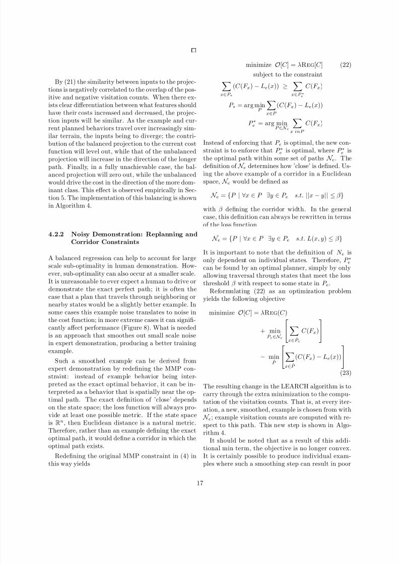
(a) Example Paths (b) Planned Paths (No Replanning) (c) Planned Paths (With Replanning)

Figure 8: An example of how noisy demonstration can hurt performance. The red and green example pathsin (a) are slightly too close to trees, preventing the cost of the trees from increasing sufficiently to matchthe red example (map (b)). However, if the paths are allowed to be replanned within a corridor, the redand green path are essentially smoothed, allowing the cost of trees to get sufficiently high (map (c)). Onaverage, the trees achieve three times the cost in (c) as in (b).

local minima; however, it has been observed empiri-cally that this effect is neutralized when using multi-ple examples. The experimental performance of thissmoothing step is presented in Section 5.

When operating with dynamic and partially un-known perceptual data, this replanning step providesanother important side effect. Rewriting (17) withthis additional min term yields


+Xt

minP te∈N

te

0@ X

x∈P te∩Vt

C (F tx) +X

x∈P te∩Vt

C V(x)

1A

−Xt

minP t

0@ Xx∈P t∩Vt

(C (F tx) − Lte(x)) +X

x∈P t∩Vt

C V(x)1A

Where N te is the set of paths near P te . However, asbefore it should be noted that the C V terms will haveno affect on the functional gradient. Therefore, thedefinition of N te does not need to consider states inV . This yields the following general definition of N te

N te = {P t | ∀x ∈ P t

V t ∃y ∈ P te

V ts.t. L(x, y) ≤ β }

the result is that N t

e only defines closeness over V t

.Behavior outside of V t does not directly affect thegradient, but does affect the objective value (the dif-ference in cost between the current (replanned) exam-ple and planned behavior). Therefore, by performinga replanning step (even with β = 0), example be-havior can be made consistent with C V without com-promising its effectiveness as an example within V t.This notion of consistency proves to have meaningfulvalue.

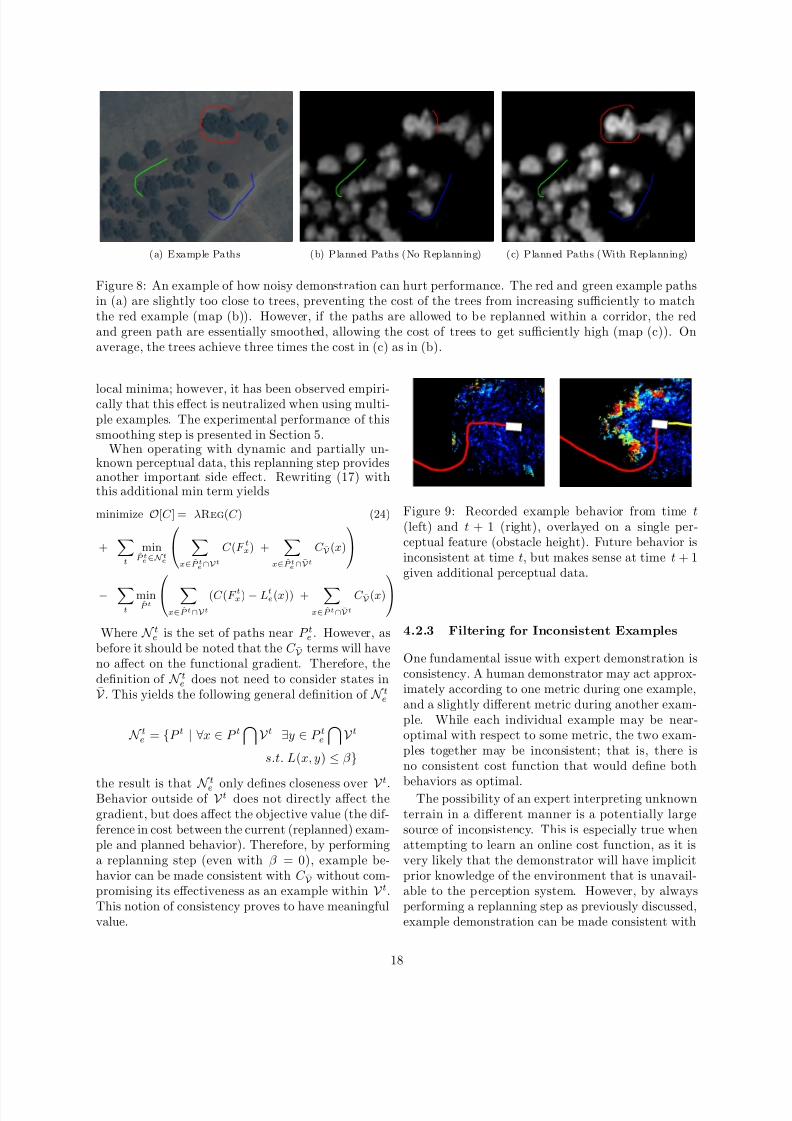
Figure 9: Recorded example behavior from time t(left) and t + 1 (right), overlayed on a single per-ceptual feature (obstacle height). Future behavior isinconsistent at time t, but makes sense at time t + 1given additional perceptual data.

4.2.3 Filtering for Inconsistent Examples

One fundamental issue with expert demonstration isconsistency. A human demonstrator may act approx-imately according to one metric during one example,and a slightly different metric during another exam-ple. While each individual example may be near-optimal with respect to some metric, the two exam-ples together may be inconsistent; that is, there isno consistent cost function that would define both

behaviors as optimal.The possibility of an expert interpreting unknown

terrain in a different manner is a potentially largesource of inconsistency. This is especially true whenattempting to learn an online cost function, as it isvery likely that the demonstrator will have implicitprior knowledge of the environment that is unavail-able to the perception system. However, by alwaysperforming a replanning step as previously discussed,example demonstration can be made consistent with

18



the robot’s interpretation of the environment in un-observed regions.

With consistency in unobserved regions accountedfor, there remain four primary sources of inconsistentdemonstration

•Inconsistency between multiple experts

• Expert error (poor demonstration)

• Inconsistency between an expert’s and therobot’s perception in observed regions

• A mismatch between an expert’s planned andactual behavior

This last issue was alluded to in Section 4.1: whilean expert example should consist of an expert’s plan at time t from the current state to the goal, what isrecorded is the expert’s behavior from time t to thegoal. Figure 9 provides a simple example of this mis-

match: at time t, the expert likely planned to drivestraight, but was forced to replan at time t + 1 whenthe cul-de-sac was observed. This breaks the assump-tion that the expert behavior from time t onwardmatches the expert plan; the result is that the dis-cretized example at time t is inconsistent with otherexample timesteps.

However, the very inconsistency of such timestepsprovides a basis for their filtering and removal.Specifically, it can be assumed that a human expertwill plan in a fairly consistent manner during a sin-gle example traverse7. If the behavior from a singletimestep or small set of timesteps is inconsistent withthe demonstrated behavior at other timesteps, thenit is safe to assume that this small set of timestepsdoes not demonstrate correct behavior, and can befiltered out and removed as training examples. Thisdoes not significantly affect the amount of trainingdata required to train a full system., as by definitionan inconsistent timestep is unlikely to provide an ex-ample of an important concept.

Inconsistency can be quantitatively defined by ob-serving each timestep’s contribution to the objectivefunctional (its slack penalty). In (5) this penalty isexplicitly defined as a a measurement of by how much

a constraint remains violated. If the penalty at a sin-gle timestep of an example behavior is a statisticaloutlier from the distribution of slack penalties at allother timesteps, it indicates that single timestep im-plies constraints that remain violated far more thanothers. That is, the constraints at an outlier timestepare inconsistent with those implied by the rest of ademonstration.

7If this assumption does not hold, then the very idea of learning from said expert’s demonstration is flawed

Therefore, the following filtering heuristic is pro-posed as a pre-processing step. First, attempt tolearn a cost function over all timesteps of a singleexample behavior and identify statistical outliers (ac-cording to slack penalties). During this step, a morecomplex hypothesis space of cost functions should

be used than is intended for the final cost function(i.e use more complex regressors). As these outliertimesteps are inconsistent within an overly complexhypothesis space, there is evidence that the incon-sistency is in the example itself, and not for lack of expressiveness in the cost function. Therefore, thesetimesteps should be removed. This process can berepeated for each example behavior, with only re-maining timesteps used in the final training.

Aside from filtering out inconsistency due toplan/behavior mismatch, this approach will also fil-ter timesteps due to other sources of inconsistency.This is beneficial, as long as the timesteps truly are

inconsistent. However, the possibility always remainsthat the example itself was correct; it may only ap-pear inconsistent due to the fidelity of perception orplanning. In this case, filtering is still beneficial, asthe examples would not have been learnable (withthe current set of perceptual features and the currentplanning system); instead, the small subset of filteredexamples can be examined by a system expert, whomay then identify a necessary additional componentlevel capability. Experimental results of this filteringapproach are presented in Section 5.

4.3 Application to Mobile RoboticSystems

Before LEARCH (in either its static or dynamicforms) can be applied to the task of learning a ter-rain cost function for a mobile robotic system, thereare still some practical considerations to address. Itis important to remember the specific task for whichLEARCH is intended: it is designed to select a costfunction from a defined hypothesis space C , such thatexpert demonstration is recreated when the cost func-tion is applied to the specific perception and planningsystems for which it was trained. There are several

hidden challenges in that statement, such as definingC, and ensuring LEARCH is producing a cost func-tion for the correct planning system.

4.3.1 Selecting a Cost Function Hypothesis

Space

The cost function hypothesis space C is implicitly de-fined by the regressor space R. In turn, R is definedby design choices relating to the family and allowable

19



Figure 10: Example of a new feature (right) learnedautomatically from panchromatic imagery (left) usingonly expert demonstration (there are no explicit classlabels).

complexity of regressors. For example, if single layer

neural networks with at most H hidden are chosenas the class of regressors, than C consists of all costfunctions that are a weighted sum of such networks.In this way, cost functions of almost arbitrary com-plexity can be allowed.

However, as with most machine learning tech-niques, there is a design tradeoff between expressive-ness and generalization. Complex regressors are ca-pable of expressing complex costing rules, but aremore prone to overfitting. In contrast, simpler re-gressors may generalize better, but are also limitedin the costing rules they can express. This tradeoff must be effectively balanced to ensure both sufficientexpressiveness and generalization. Fortunately, as re-gression is a core machine learning task, there are welldeveloped and understood approaches for achievingthis balance. In practice, validation with an inde-pendent holdout set of demonstrated behaviors canhelp quantify this tradeoff. This allows a range of regressor types and complexities to be automaticallyevaluated; the one with the best holdout performancecan be selected with minimal additional human inter-action.

Another issue with respect to the definition of C iscomputational cost. In a scenario where perceptual

features are static, this concern is not as important,as cost evaluations are only performed once. How-ever, in an online and dynamic setting, cost eval-uations are performed continuously; computationalcomplexity may be a much larger issue. As the finallearned cost function is a weighted combination of K regressors, computational complexity of the final costfunction is linear in K . Again, this creates a designtradeoff; limiting K will limit the computational costper evaluation, but will also limit the accuracy of the

cost function (as the final steps of a gradient descentoperation fine tune the solution).

One solution is to define R as the space of linearfunctions. Since the weighted sum of linear func-tions is another linear function, using this defini-tion of R would result in the final complexity of

C K being constant with respect to K . However us-ing linear regressors with LEARCH results in almostthe same solution as would be produced by the lin-ear MMP algorithm (but not identical due to expo-nentiated functional gradient descent). As the fun-damental advantage of the LEARCH approach wasto allow non-linear cost functions, this would seemto imply a necessary tradeoff. However, the addi-tion of a feature learning phase [Ratliff et al., 2007,Silver et al., 2008, Silver et al., 2009a] to LEARCHcan potentially solve this problem. During mostlearning iterations, linear regressors are used. How-ever, when it is detected that the objective error is no

longer decreasing, a single, simple non-linear regres-sion is performed. This single, non-linear step wouldbetter discriminate between terrains that are difficultfor a purely linear regressor. However, rather thanadd this new regressor directly into the cost func-tion, it is instead treated as a new feature. Figure 10provides a simple example of a learned feature withonly greyscale imagery as input.

4.3.2 Planner Interpretation of Cost Maps

A common approach in mobile robotics is to treat theenvironment as a 2.5D space; this allows the statespace S for high level path planning to be R2. Thisresults in terrain costs defined over a a discretized2D grid. However, different planning systems mayinterpret a 2D cost grid differently. Since the goal isto learn a cost function to recreate behavior with aspecific planning system, these details must be takeninto account to learn the cost function correctly.

Perhaps the simplest cost-aware planner one mightuse for a mobile robot would be 4-connected A* (orother grid planner). Such a planning system wouldincur a cost of C (x) whenever a cell x was traversed.Now consider the case of an 8-connected A*. Many

8-connected implementations treat traversing a celldiagonally as higher cost than traversing the samecell axis-aligned; this allows the planner to take intoaccount the extra distance traversed through a grid.This usually takes the form of incurring a cost of C (x)when traversing the cell axis-aligned, and a cost of √

2C (x) when traversing the cell diagonally.

Since cells traversed diagonally incur more cost,this must be taken into account by LEARCH whencomputing the projection of the functional gradient.

20



With respect to the final cost of a path, a cell tra-versed diagonally will have a

√2 greater affect than

one traversed axis-aligned; therefore it is√

2 timesmore important to get the sign right on the projec-tion. The solution is to increment the visitation countof a cell by 1 when traversing it axis-aligned, and by

√2 when traversing diagonally. In the general case,a planner may incur a cost of dC (x) when traversinga distance d through cell x; the visitation count of state x should then be incremented by d.

Another issue that must be considered is that of configuration space expansion. Motion planners formobile robotic systems often apply a c-space expan-sion to an input cost map before generating a plan,in order to account for the physical dimensions of therobot. The result is that the cost the planner assignsfor traversing distance d through state x is no longerdC (x), but rather something along the lines of

d

y∈N

W (x, y)C (y) (25)

where N is a set of states sufficiently close to x, andW is a weighting function. Common choices for W in-clude a constant, or a linear falloff based on ||x − y||.As before, this weighting must be captured by thevisitation counts: if distance d is traversed throughcell x, then all cells y ∈ N must have there visitationcounts incremented by dW (x, y). A further compli-cation arises if W depends not only on the locationsof x and y, but also their (or other states) cost values.For instance, if a c-space expansion defined the cost

of traversing d through state x as

d maxy∈N

C (y)

then only the state y with the maximum cost in N should have its visitation count incremented by d; allother states would not affect the planner perceivedcost of traversing x under the current C . Unlike (25),this form results in non-convexity in the LEARCHalgorithm (in addition to non-convexity from replan-ning), as different initial cost functions C 0 may pro-duce significantly different results.

4.3.3 Planners with Motion Constraints

A common architecture for mobile robot planningsystems is to utilize a hierarchy of planners, rang-ing from long-range low resolution planners to short-range high resolution planners. The simplest formof this architecture utilizes a long-range, uncon-strained ’global’ planner, and a short-range, kine-matically or dynamically constrained ’local’ planner

[Kelly et al., 2006, Stentz et al., 2007]. Usually, a lo-cal planner does not plan all the way to the goal; in-stead it produces a set of feasible short-range actions,and utilizes the global planner to produce a path fromthe end of the action to the goal. Local planner gen-erated plans are not actually followed to completion,

but instead are replanned at a high rate. In this way,the local planner is not actually optimal, but insteadperforms something akin to a greedy search.

If LEARCH is to be used for an onboard percep-tion system, it is important that they be learned withrespect to the planning system that will be used on-board the robot. If a hybrid architecture is used,LEARCH must therefore be implemented using thesame configuration. It is important that the decisionsthe planner is tasked with making during training areexactly those that will be required during operation.For example, in the case of a greedy local planningsystem, P t∗ at each iteration should be the direct out-

put of the planning system, not the concatenation of multiple planning cycles (even though this is how therobot’s behavior is determined online). This is nec-essary for credit assignment; if at time t the expertswerved to avoid an obstacle, then not only must thecost of the obstacle be sufficiently high, but the costof the terrain swerved over must be sufficiently low.Even if subsequent actions reduce the distance trav-eled during the swerve, the planner must be willingto perform a large turn at time t to begin that ma-neuver.

Related to this issue is one of planner fidelity. De-pending on discretization resolution and the level of vehicle modeling, it is unlikely that a kinematically ordynamically constrained planning system will be ableto exactly recreate the same behavior as executedduring demonstration. Inability to recreate demon-strated behavior can introduce noise into the learnedcost function, of magnitude proportional to the de-gree of mismatch. Possible solutions for this issueare discussed in the next two sections.

5 Experimental Results

Learning cost functions by demonstration was appliedto the Crusher autonomous system (Figure 1). TheCrusher vehicle is capable of traversing rough, com-plex, and unstructured terrain; as such understandingthe relative benefits and tradeoffs of various terraintypes is of paramount importance to its autonomousoperation. On Crusher, terrain data comes from twoprimary sources. The first is prior, static, overheaddata sources (satellite or aerial imagery, aerial Li-DAR, etc.). Overhead data is processed via a set

21



Figure 11: A high level block diagram of the CrusherAutonomy system

of engineered feature extractors into a set of featuremaps, which are then mapped into a single, staticcostmap for an entire area of operation. The sec-ond source of terrain data comes from the onboardperception system. The onboard perception systemprocesses local data from onboard camera images andLiDAR into a dynamic stream of features. At a highdata rate, these features are continuously mapped tocostmaps over a local area.

Costs from both sources are continuously fused intoa single consistent costmap, which is then passedto Crusher’s motion planning system. Fusing priorand onboard perceptual data at the cost level al-lows for Crusher to continuously plan a path allthe way from its current position to the goal. Dueto the dynamic nature of this cost data, the FieldD* algorithm is utilized [Ferguson and Stentz, 2006].In order to determine feasible local motion com-mands for Crusher, a variant of the RANGER sys-tem [Kelly, 1995, Kelly et al., 2006] is applied, uti-lizing the Field D* plan for global guidance. This

architecture is shown is Figure 11.Early in Crusher’s development, the task of in-terpreting both static and dynamic perceptual datainto costs was performed through manual engineer-ing, and was a large source of frustration. This ledto the application of learning by demonstration toconstructing cost functions. This was first applied inthe static perceptual case (overhead data) utilizingthe Field D* planner, and was next applied to thedynamic case (onboard perceptual data) utilizing theField D* guided RANGER local planner. The re-mainder of this section describes these experiments,along with offline results from each task.

Two metrics are used for evaluating offline perfor-mance. The first is the average loss along a path. Asthe loss function is constructed to encode the similar-ity between two paths, the loss between an examplepath and the corresponding planned path (over theinterval [0,1]) is a measure of how accurately expertbehavior has been reproduced. A second measureis the cost ratio, defined as the cost of an examplepath divided by the cost of the corresponding plannedpath. As this ratio approaches 1, it indicates the cur-

(a) Simulated Examples

(b) Expert Drawn Examples

Figure 12: Learning simulated and expert drawn ex-

ample paths. Test set performance is shown as a func-tion of number of input paths

rent cost function hypothesis is approaching consis-tency with the expert demonstration. The cost ratioas opposed to cost difference is used to account forthe affect of scaling on the cost function (with thecost difference, simply scaling the costs closer to zerowould improve the metric, without improving the rel-ative cost difference).

5.1 Learning to Interpret Overhead

Data

In order to verify LEARCH under ideal conditions,tests were first run on simulated examples. A known(arbitrary) cost function was used to generate a costmap over a single environment from its overhead fea-tures; this cost map was used to produce paths be-tween random waypoints. Different numbers of thesepaths were then used as input for LEARCH, and theperformance measured on a large independent vali-

22



0 5 10 150.42

0.44

0.46

0.48

0.5

0.52

0.54

0.56

0.58

0.6

Corridor Size (in cells)

V a l i d

a t i o n

L o s s

Figure 13: Validation loss as a function of the corri-dor size. Using corridor constraints improves perfor-mance as long as the corridor is not too large

dation set of paths (generated in the same manner).Figure 12(a) shows the results using both the

balanced and standard weighting schemes (Section4.2.1). As the number of training paths is increased,the test set performance continues to improve. Eachinput path further constrains the space of possiblecost functions, bringing the learned function closerto the desired one. However, there are diminishingreturns as additional paths overlap to some degreein their constraints. Finally, the performance of thebalanced and standard weighting schemes is similar.Since all paths for this experiment were generated by

a planner, they are by definition optimal under somemetric, and therefore both achievable and consistentwith each other.

Next, experiments were performed with expert ex-amples (both training and validation) drawn on top of overhead data maps. Figure 12(b) shows the resultsof an experiment of the same form as that performedwith simulated examples. Again, the validation setcost ratio decreases as the number of training exam-ples increases. However, with real examples thereis a significant difference between the two weight-ing schemes; the balanced weighting scheme achievedsignificantly better performance. This demonstrates

both how human demonstration can suffer from largescale non-optimality, and how LEARCH can be maderobust to this fact through a balanced regression.

Another series of experiments were performed todetermine the effect of performing replanning withcorridor constraints (Section 4.2.2). For these ex-periments, the performance of learning was measuredwith validation loss, to indicate how well the plannedpaths matched the examples. When measuring losson the validation set, no replanning was performed.

Therefore, in order to provide a smoother metric, thespecific loss function used was a radial basis functionbetween states on the current path P ∗ and the closeststate on the example P e, with a scale parameter σ2

L(P ∗, P e) =1

|P ∗| x∈P ∗

[1

−exp( min

xi∈

P e

[

x

−xi

2]/σ2)]

Using a loss function of this form provides a more ana-log metric than a Hamming style loss as previouslydescribed. Figure 13 shows the results on the valida-tion set as a function of the corridor size (in cells).Small corridors provide an improvement over no cor-ridor, demonstrating how small scale smoothing canimprove generalization. However, as the corridor getstoo large, this improvement disappears; large corri-dors essentially over-smooth the examples and beginto miss critical information.

Finally, experiments were performed in order to

compare the offline performance of learned costmapswith engineered ones. A cost map was trained off of satellite imagery for an approximately 60 km2 sizeenvironment. An engineered costmap had been pre-viously produced for this same test site to supportCrusher operations. This engineered map was pro-duced by performing a supervised classification of theimagery, and then manually determining a cost foreach class [Silver et al., 2006]. A subset of both mapsis shown in Figure 15. The two maps were comparedusing a validation set of paths generated by a Crusherteam member not directly involved in the develop-ment of overhead costing. The average validation lossusing the LEARCH map was 23% less than the engi-neered map (Figure 14), thus demonstrating superiorgeneralization of the learned approach.

Online validation of the learned costmaps was alsoachieved during Crusher field tests. These tests con-sisted of Crusher autonomously navigating a series of courses, with each course defined as a set of widelyspaced waypoints. Courses ranged in length up to20 km, with waypoint spacing on the order of 200 to1000 m. These tests took place at numerous locationsacross the continental U.S., each with highly varyinglocal terrain characteristics, and sizes ranging from

tens to hundreds of square kilometers.During 2005 and 2006, prior maps were primarily

generated as described in [Silver et al., 2006]. An ini-tial implementation of the LEARCH algorithm wasalso field tested and demonstrated in smaller testsduring 2006. During 2007 and 2008, LEARCH be-came the default approach for producing cost maps.Overall, LEARCH maps were used during more than600 km of sponsor monitored autonomous traverse,plus hundreds of kilometers more of additional field

23



Experiment Total Net Avg. Total Cost Max CostDistance(km) Speed(m/s) Incurred Incurred

Experiment 1 6.63 2.59 11108 23.6LearnedExperiment 1 6.49 2.38 14385 264.5Engineered

Experiment 2 6.01 2.32 17942 100.2LearnedExperiment 2 5.81 2.23 21220 517.9EngineeredExperiment 2 6.19 1.65 26693 224.9No Prior

Table 1: Results of experiments comparing learned to engineered prior maps. Indicated costs are from thevehicle’s onboard perception system.

Engineered Learned

0

0.1

0.2

0.3

0.4

0.5

0.6

0.7

0.8

V a l i d a t i o n L o s s

Figure 14: Performance comparison between alearned and engineered prior costmap. The learnedmap produced behavior that better matched an in-dependent validation set of examples.

testing. This demonstrates that a learned cost func-tion was sufficient for use online a complex roboticsystem.

In addition, two direct online comparisons were

performed. These two tests were performed severalmonths apart, at different test sites. During eachexperiment, the same course was run twice, vary-ing only the prior cost map given to the vehicle be-tween runs. The purpose of these experiments wasto demonstrate that learning a cost function not onlygeneralized better with respect to initial route plan-ning, but also with respect to dynamic replanningonline.

Each run was scored according to the total cost

incurred by the vehicle according to its onboard per-

ception system. At the time of these experiments, theperception system made use of a manually engineeredcost function. However, this function was shownthrough numerous experiments [Stentz et al., 2007]to result in a high level of autonomous performance;therefore it is a valid metric for scoring the safety of a single autonomous run.

The results of these experiments are shown in Ta-ble 1. In both experiments, the vehicle traveled far-ther to complete the same course using learned priordata, and yet incurred less total (online) cost. Overboth experiments, with each waypoint to waypointsection considered an independent trial, the improve-

ment in average cost and average speed is statisti-cally significant at the 5% and 10% levels, respec-tively. This indicates that the terrain the vehicle tra-versed was on average safer when using the learnedprior map, according to its own onboard perceptionsystem. This normalization by distance traveled isnecessary because the learned prior and engineeredperception cost functions do not necessarily agree inwhat they consider unit cost. Additionally, the max-imum cost incurred at any point along an experimentis also provided; for both terrains, the maximum issignificantly lower when using the learned prior data.The course for Experiment 2 was also run withoutany prior data; the results are presented for compar-ison.

In addition to improving vehicle performance, us-ing learned cost functions also reduced the necessaryamount of human interaction. When preparing for aCrusher test using engineered costmaps, performinga supervised classification and tuning the cost func-tion would take on the order of 1-2 days. In contrast,when using learned costmaps drawing example paths

24



Figure 15: A 10 km2 section of a Crusher test site.From top to bottom: Quickbird imagery, LearnedCost, and Engineered Cost

would require on the order of 1-2 hours8. In a timedhead-to-head experiment on a 2 km2 test site, pro-ducing a supervised classification required 40 minutesof expert involvement, and tuning a cost function re-quired an additional 20 minutes. In contrast, produc-ing example paths required only 12 minutes. On thissame experiment, the learned costmap had a valida-tion loss of 0.43, compared to 0.56 for the engineeredmap. This demonstrates that the learned approach

8Neither of these timings include the necessary effort toprocess raw overhead data into feature maps, as this processis a shared precursor to both approaches to costing

EngineeredLearned (w/class)

Learned(wo/class)

0

10

20

30

40

50

60

70

0

0.1

0.2

0.3

0.4

0.5

0.6

Loss

Time

T i m e ( m i n u t e s )

V a l i d a t i o n

L o s s

Figure 16: Performance comparison between 3 ap-proaches to generating prior costmaps. LEARCH notonly performs better and faster at the task of deter-mining costs of different semantic classes, it also doesa better job at interpreting raw data (for the purposeof costing) than semantic classification.

produced superior performance, with less human in-teraction time (Figure 16).

An additional test was performed in which thesame training set of example paths was used to learna cost function only from the results of the supervisedclassification; in this case the learned map had a vali-dation loss of 0.52. This demonstrates two importantpoints. The first is that even when the problem of learning a cost function was reduced to solely a lowdimensional parameter tuning problem (in this case5 dimensions), the automated approach was able toperform better than manual tuning, and with lesshuman interaction. The second point is that reduc-ing the task to a lower dimensional problem (labelingfor the supervised classification) required additionalinteraction, and that this feature space compressionresulted in a loss of useful information (as the val-idation loss was better when learning from the fullfeature space as opposed to the compressed one).

5.2 Learning to Interpret Online Per-

ceptual Data

Next, dynamic LEARCH was applied to the task of learning a cost function for Crusher’s onboard percep-tion system (Figure 17). Training data in the formof expert example behaviors was gathered by havingCrusher’s safety operator RC the vehicle through setsof waypoints. Different training examples were col-lected over a period of months in varying locationsand weather conditions, and with 3 different oper-ators at one time or another. During data collec-

25



0 20 40 60 80 100 120 140 160 180 2000.55

0.6

0.65

0.7

0.75

0.8

iteration

v a l i d a t i o n

l o s s

unbalanced

balanced

0 20 40 60 80 100 120 140 160 1800.588

0.59

0.592

0.594

0.596

0.598

0.6

0.602

0.604

corridor size in cm

v a l i d a t i o n

l o s s

0 1 2 3 4 5 6 7 8 9

0.57

0.575

0.58

0.585

0.59

0.595

0.6

0.605

0.61

Number of Regression Trees

v a l i d a t i o n

l o s s

Figure 18: Results of offline experiments on logged perception data. Left: Validation Loss during learningfor the balanced and standard weighting Center: Validation Loss as a function of the replanning corridorsize Right: Validation Loss as a function of the number of regression trees.

tion, all raw sensor data was logged along with theexample path. Perceptual features were then pro-duced offline by feeding the raw sensor data through

Crusher’s perception software. In this way, the baseperception system and its features could be modifiedand improved without having to recollect new train-ing data; the raw data is just reprocessed, and a costfunction learned for the new features.

This set of examples was first used to perform aseries of offline experiments to validate the dynamicextension of LEARCH. Loss on a validation set wasused as the metric, to measure how well planned be-havior recreated example behavior. These results arepresented in Figure 18. The left graph again demon-strates the effectiveness of performing balanced as op-posed to unbalanced regression, as the balanced ver-sion has superior validation performance. The centergraph further demonstrates the utility of replanningwith corridor constraints. With a small corridor size,the algorithm is able to smooth out some of the noisein example human behavior, and improve generaliza-tion. As the corridor size increases, the algorithmbegins to over-smooth, resulting in decreasing valida-tion performance. This also demonstrated how vali-dation data can be used to automatically determinethe optimal corridor size.

An experiment was also performed to assess the ef-fectiveness of filtering out inconsistent timesteps. A

single expert behavior was used to learn a cost func-tion, first with no filtering, and then with approx-imately 10% of its timesteps automatically filtered.As would be expected, the performance of the re-maining 90% of the training set improved after filter-ing (Figure 19). However, performance on the vali-dation set also improved slightly. This demonstratesthat filtering out inconsistent timesteps non only im-proves performance on examples for which the filteredtimesteps were inconsistent, it also improves general-

ization to unseen examples.

As cost evaluations in an onboard perception sys-tem must be performed in real time, the computa-

tional cost of an evaluation is an important consid-eration. As described in (Section 4.3.1), using onlylinear regressors is beneficial from a computationalstandpoint, and feature learning can be used to im-prove the complexity of the cost function if necessary.Figure 18 (Right) shows validation loss as a functionof the number of added features learned using simpleregression trees. At first, additional features improvesthe validation performance; however, eventually toomany features can cause overfitting.

Next, the collected training set was used to learna cost function to run onboard Crusher. Originally,

Crusher used an engineered perception cost func-tion. During more than 3 years of Crusher develop-ment, this cost function was continually redesignedand retuned, culminating in a high performance sys-tem [Stentz et al., 2007]. However, this performancecame at a high cost of human effort. Version con-trol logs indicate that 145 changes were made to justthe structure of the model mapping perceptual fea-tures to costs; additionally more than 300 parameterchanges were checked in (untold more were tried atone point or another, requiring verification on loggeddata or actual vehicle performance). As each com-mitted change requires significant time to design, im-

plement, and validate, easily hundreds of hours werespent on engineering the cost function. In contrast,the time to collect the final training set for learningby demonstration required only a few hours of hu-man time (spread over several months). This seem-ingly small amount of human demonstration is suf-ficient due to the numerous constraints implied byeach example behavior: the approximately 3 kilome-ters of demonstration provides hundreds of thousandsof examples of states to traverse, and millions more

26



(a) Left Camera Image (b) Right Camera Image

(c) Max Object Height (d) Density in Wheel Re-gion

(e) Density in Hull Region (f) Density above Vehicle

(g) Solid Classification (h) Learned Cost

Figure 17: An example of learned perception costfrom a simple scene, depicted in (a),(b). Processing

of raw data results in perceptual features (a subset of which are shown in (c) - (g)) that are mapped intocost (h) by a learned function.

Training Loss Validation Loss

0

0.1

0.2

0.3

0.4

0.5

0.6

0.7

With Filtering

No Filtering

Figure 19: Comparison of performance with andwithout filtering. Filtering out inconsistent timestepsimproves performance on both training examplewhich were inconsistent with the filtered examples,

as well as on an independent validation set.

examples of states that were avoided.

Crusher’s perception system actually consists of two modules: a local perception system that pro-duces high resolution cost data out to 20m, and afar range perception system that produces mediumresolution cost data out to 60m. The far rangesystem utilizes near-to-far learning as described in[Sofman et al., 2006] for learning a far range costfunction from near range cost data. Therefore, whenthe system learns online from scratch, the near rangecost function implicitly defines the far range costfunction. For this reason, learning by demonstra-tion was only used to learn the near range function;the far range function would automatically adapt towhatever near range function was utilized.

As Crusher utilizes a hybrid local/global plan-ning architecture, it was necessary to learn a costfunction with respect to the lowest level of motionplanning (see Section 4.3.3); otherwise the learnedcost function would not actually recreate demon-strated behaviors when applied online. However,the local planner suffers from low fidelity; while

the concatenation of multiple planning cycles canproduce behavior of surprising complexity, indi-vidual planning cycles consider only a relativelysmall subset of possible actions. This approachhas proven quite effective on Crusher, as well as inprevious off road mobile systems [Singh et al., 2000,Kelly et al., 2006, Biesiadecki and Maimone, 2006,Carsten et al., 2009]. Unfortunately, as previouslystated this inability for the planner to recreatedemonstrated behavior in a single planning cycle can

27





System Avg Dist Avg Cmd Avg Cmd Avg Lat Dir Switch Avg MotorMade Good (m) Vel (m/s) Ang Vel.(◦/s) Vel (m/s) Per m Current (A)

Engineered 130.7 3.24 6.56 0.181 0.107 7.53

Global 123.8* 3.34* 4.96* 0.170* 0.081* 7.11*Local 127.3 3.28 5.93* 0.172* 0.100 7.35

Local w/replan 124.3* 3.39* 5.08* 0.170* 0.082* 7.02*

System Avg Avg Avg Vert Avg Lat Susp SafetyRoll(◦) Pitch(◦) Accel (m/s2) Accel (m/s2) Max∆ (m) E-stops

Engineered 4.06 2.21 0.696 0.997 0.239 0.027

Global 4.02 2.22 0.710* 0.966* 0.237 0.054*

Local 4.06 2.22 0.699 0.969* 0.237 0.034Local w/replan 3.90* 2.18 0.706* 0.966* 0.234* 0.030

Table 2: Averages over 295 different waypoint to waypoint trials per perception system, totaling over 150kmof traverse. Statistically significant differences (from Engineered) denoted by *

ism for how a cost function should be defined; it is thesimplest function that meets constraints implied by

example behavior. As opposed to a hand tuned ap-proach (which can easily overfit) this simplicity pro-vides a theoretical basis for achieving robustness andgeneralization. Further, this approach naturally re-sults in an automated framework for both initial andcontinuing cost function validation.

Future work will explore the application of this ap-proach to learning cost functions over full state-actionpairs. The behavior of an autonomous navigationsystem is defined not only by which terrain it prefers,but by which motions it prefers (e.g. minimum cur-vature). Improper modeling of these preferences is

just as significant a detriment to robot performanceas improper modeling of terrain preferences; it alsocontributes to the inability of some planning systemsto properly recreate demonstrated behavior. Previ-ous work [Abbeel et al., 2008] has briefly investigatedthis challenge independently of the equivalent percep-tion problem. However, by learning all preferencesat once from human demonstration, we hope to fur-ther improve the robustness of autonomous naviga-tion, while further reducing the effort involved in de-ployment and validation of such systems.

AcknowledgmentsThis work was sponsored by DARPA under contract“Unmanned Ground Combat Vehicle - PerceptORIntegration” (contract MDA972-01-9-0005) and bythe U.S. Army Research Laboratory under contract“Robotics Collaborative Technology Alliance” (con-tract DAAD19-01-2-0012). The views and conclu-sions contained in this document are those of the au-thors and should not be interpreted as representing

the official policies, either expressed or implied, of theU.S. Government. Additionally, the authors would

like to thank the many members of the Crusher ve-hicle and autonomy teams who made this work pos-sible.

References

[Abbeel et al., 2008] Abbeel, P., Dolgov, D., Ng,A. Y., and Thrun, S. (2008). Apprenticeship learn-ing for motion planning with application to park-ing lot navigation. In International Conference on Intelligent Robots and Systems.

[Abbeel and Ng, 2004] Abbeel, P. and Ng, A. Y.(2004). Apprenticeship learning via inverse rein-forcement learning. In International Conferenceon Machine learning .

[Angelova et al., 2007] Angelova, A., Matthies, L.,Helmick, D., and Perona, P. (2007). Learning andprediction of slip from visual information. Journal of Field Robotics, 24(3):205–231.

[Bagnell et al., 2010] Bagnell, J., Bradley, D., Silver,D., Sofman, B., and Stentz, A. (2010). Learn-ing rough-terrain autonomous navigation. IEEE Robotics and Automation Magazine.

[Bajracharya et al., 2008] Bajracharya, M., Tang,B., Howard, A., Turmon, M., and Matthies, L.(2008). Learning long-range terrain classificationfor autonomous navigation. In IEEE International Conference on Robotics and Automation , pages4018–4024.

[Balakirsky and Lacaze, 2000] Balakirsky, S. and La-caze, A. (2000). World modeling and behavior gen-

29



eration for autonomous ground vehicle. In Proceed-ings IEEE International Conference on Roboticsand Automation , volume 2, pages 1201–1206.

[Biesiadecki and Maimone, 2006] Biesiadecki, J. andMaimone, M. (2006). The mars exploration roversurface mobility flight software driving ambition.In IEEE Aerospace Conference.

[Bradley et al., 2007] Bradley, D., Unnikrishnan, R.,and Bagnell, J. A. (2007). Vegetation detection fordriving in complex environments. In International Conference on Robotics and Automation .

[Buehler, 2006] Buehler, M. (2006). Summary of dgc2005 results. Journal of Field Robotics, 23:465–466.

[Carsten et al., 2009] Carsten, J., Rankin, A., Fer-guson, D., and Stentz, A. (2009). Global planningon the mars exploration rovers: Software integra-

tion and surface testing. Journal of Field Robotics,26:337–357.

[Dahlkamp et al., 2006] Dahlkamp, H., Kaehler, A.,Stavens, D., Thrun, S., and Bradski, G. (2006).Self-supervised monocular road detection in desertterrain. In Proceedings of Robotics: Science and Systems, Philadelphia, USA.

[Dima et al., 2004] Dima, C., Vandapel, N., andHebert, M. (2004). Classifier fusion for outdoorobstacle detection. In International Conference on Robotics and Automation , volume 1, pages 665 –671. IEEE.

[Ferguson and Stentz, 2006] Ferguson, D. andStentz, A. (2006). Using interpolation to improvepath planning: The field D* algorithm. Journal of Field Robotics, 23(2):79–101.

[Hadsell et al., 2009] Hadsell, R., Sermanet, P., Ben,J., Erkan, A., Scoffier, M., Kavukcuoglu, K.,Muller, U., and LeCun, Y. (2009). Learning long-range vision for autonomous off-road driving. Jour-nal of Field Robotics, 26:120–144.

[Halatci et al., 2007] Halatci, I., Brooks, C., and Iag-nemma, K. (2007). Terrain classification and clas-sifier fusion for planetary exploration rovers. InIEEE Aerospace Conference.

[Hamner et al., 2006] Hamner, B., Singh, S., andScherer, S. (2006). Learning obstacle avoidance pa-rameters from operator behavior. Journal of Field Robotics, 23(1):1037–1058.

[Happold and Ollis, 2007] Happold, M. and Ollis, M.(2007). Using learned features from 3d data for

robot navigation. Autonomous Robots and Agents,76:61–69.

[Helmick et al., 2009] Helmick, D., Angelova, A.,and Matthies, L. (2009). Terrain adaptive naviga-tion for planetary rovers. Journal of Field Robotics,26:391–410.

[Howard et al., 2007] Howard, A., Turmon, M.,Matthies, L., Tang, B., Angelova, A., and Mjol-sness, E. (2007). Towards learned traversability forrobot navigation: From underfoot to the far field.Journal of Field Robotics, 23:1005–1017.

[Howard et al., 2005] Howard, A., Werger, B., andSeraji, H. (2005). A human-robot mentor-protegerelationship to learn off-road navigation behav-ior. In IEEE International Conference on Systems,Man and Cybernetics, volume 1, pages 430–435Vol. 1.

[Huertas et al., 2005] Huertas, A., Matthies, L., andRankin, A. (2005). Stereo-based tree traversabil-ity analysis for autonomous off-road navigation. InSeventh IEEE Workshops on Application of Com-puter Vision , volume 1, pages 210–217.

[Iagnemma et al., 1999] Iagnemma, K., Genot, F.,and Dubowsky, S. (1999). Rapid physics-basedrough-terrain rover planning with sensor and con-trol uncertainty. In IEEE Internation Conferenceon Robotics and Automation .

[Iagnemma et al., 2004] Iagnemma, K., Kang, S.,

Shibly, H., and Dubowsky, S. (2004). Onlineterrain parameter estimation for wheeled mobilerobots with application to planetary rovers. IEEE Transactions on Robotics, 20(5):921–927.

[Kalman, 1964] Kalman, R. (1964). When is a linearcontrol system optimal? Trans. ASME, J. BasicEngrg., 86:51–60.

[Karlsen and Witus, 2007] Karlsen, R. and Witus,G. (2007). Terrain understanding for robot navi-gation. In IEEE/RSJ International Conference on Intelligent Robots and Systems, pages 895–900.

[Kelly, 1995] Kelly, A. (1995). An Intelligent Pre-dictive Control Approach to the High-Speed Cross-Country Autonomous Navigation Problem . PhDthesis, Robotics Institute, Carnegie Mellon Univer-sity.

[Kelly et al., 2006] Kelly, A., Stentz, A., Amidi, O.,Bode, M., Bradley, D., Diaz-Calderon, A., Hap-pold, M., Herman, H., Mandelbaum, R., Pilarski,T., Rander, P., Thayer, S., Vallidis, N., and

30



Warner, R. (2006). Toward reliable off road au-tonomous vehicles operating in challenging envi-ronments. International Journal of Robotics Re-search , 25(5-6):449–483.

[Kim et al., 2006] Kim, D., Sun, J., Oh, S. M., Rehg,J., and Bobick, A. (2006). Traversability classifi-cation using unsupervised on-line visual learningfor outdoor robot navigation. In Proceedings IEEE International Conference on Robotics and Automa-tion , pages 518–525.

[Lacaze et al., 2002] Lacaze, A., Murphy, K., andDelgiorno, M. (2002). Autonomous mobility for thedemo iii experimental unmanned vehicles. In in As-soc. for Unmanned Vehicle Systems Int. Conf. on Unmanned Vehicles (AUVSI 02 .

[Lalonde et al., 2006] Lalonde, J.-F., Vandapel, N.,Huber, D., and Hebert, M. (2006). Natural ter-

rain classification using three-dimensional ladardata for ground robot mobility. Journal of Field Robotics, 23(10):839–861.

[LeCun et al., 2006] LeCun, Y., Muller, U., Ben, J.,Cosatto, E., and Flepp, B. (2006). Off-road obsta-cle avoidance through end-to-end learning. In Ad-vances in Neural Information Processing Systems18 . MIT Press.

[Manduchi et al., 2005] Manduchi, R., Castano, A.,Talukder, A., and Matthies, L. (2005). Obstacledetection and terrain classification for autonomous

off-road navigation. Autonomous Robots, 18:81–102.

[Mason et al., 2000] Mason, L., Baxter, J., Bartlett,P., and Frean, M. (2000). Boosting algorithms asgradient descent. In Advances in Neural Informa-tion Processing Systems 12 , Cambridge, MA. MITPress.

[Ng and Russell, 2000] Ng, A. Y. and Russell, S.(2000). Algorithms for inverse reinforcement learn-ing. In Proc. 17th International Conf. on MachineLearning .

[Olin and Tseng, 1991] Olin, K. and Tseng, D.(1991). Autonomous cross-country navigation: anintegrated perception and planning system. IEEE Expert , 6(4):16–30.

[Ollis et al., 2007] Ollis, M., Huang, W. H., and Hap-pold, M. (2007). A bayesian approach to imitationlearning for robot navigation. In Proceedings of theIEEE/RSJ International Conference on Intelligent Robots and Systems.

[Pomerleau, 1989] Pomerleau, D. (1989). Alvinn: anautonomous land vehicle in a neural network. Ad-vances in neural information processing systems 1,pages 305 – 313.

[Procopio et al., 2007] Procopio, M., Mulligan, J.,and Grudic, G. (2007). Long-term learning us-ing multiple models for outdoor autonomous robotnavigation. In IEEE/RSJ International Confer-ence on Intelligent Robots and Systems, pages3158–3165.

[Rasmussen, 2002] Rasmussen, C. (2002). Combin-ing laser range, color, and texture cues for au-tonomous road following. In IEEE Conference on Robotics and Automation .

[Ratliff et al., 2006] Ratliff, N., Bagnell, J. A., andZinkevich, M. (2006). Maximum margin planning.In International Conference on Machine Learning .

[Ratliff et al., 2007] Ratliff, N., Bradley, D., Bagnell,J. A., and Chestnutt, J. (2007). Boosting struc-tured prediction for imitation learning. In Ad-vances in Neural Information Processing Systems19 , Cambridge, MA. MIT Press.

[Ratliff et al., 2009] Ratliff, N. D., Silver, D., andBagnell, J. A. (2009). Learning to search: Func-tional gradient techniques for imitation learning.Autonomous Robots.

[Seraji and Howard, 2002] Seraji, H. and Howard,A. (2002). Behavior-based robot navigation on

challenging terrain: A fuzzy logic approach.IEEE Transactions on Robotics and Automation ,18(3):308–321.

[Shneier et al., 2008] Shneier, M., Chang, T., Hong,T., Shackleford, W., Bostelman, R., and Albus,J. (2008). Learning traversability models for au-tonomous mobile vehicles. Autonomous Robots,24:69–86.

[Silver et al., 2008] Silver, D., Bagnell, J. A., andStentz, A. (2008). High performance outdoor nav-igation from overhead data using imitation learn-

ing. In Proceedings of Robotics Science and Sys-tems.

[Silver et al., 2009a] Silver, D., Bagnell, J. A., andStentz, A. (2009a). Applied imitation learning forautonomous navigation in complex natural terrain.In Field and Service Robotics.

[Silver et al., 2009b] Silver, D., Bagnell, J. A., andStentz, A. (2009b). Perceptual interpretation forautonomous navigation through dynamic imitation

31



learning. In International Symposium on RoboticsResearch .

[Silver et al., 2006] Silver, D., Sofman, B., Vandapel,N., Bagnell, J. A., and Stentz, A. (2006). Experi-mental analysis of overhead data processing to sup-port long range navigation. In Proceedings of theIEEE/JRS International Conference on Intelligent Robots and Systems.

[Singh et al., 2000] Singh, S., Simmons, R., Smith,T., Stentz, A., Verma, V., Yahja, A., and Schwehr,K. (2000). Recent progress in local and globaltraversability for planetary rovers. IEEE Confer-ence on Robotics and Automation .

[Sofman et al., 2006] Sofman, B., Ratliff, E. L., Bag-nell, J. A., Cole, J., Vandapel, N., and Stentz,A. (2006). Improving robot navigation throughself-supervised online learning. Journal of Field

Robotics, 23(12).

[Stavens and Thrun, 2006] Stavens, D. and Thrun,S. (2006). A self-supervised terrain roughness esti-mator for off-road autonomous driving. In In Proc.of Conf. on Uncertainty in AI , pages 13–16.

[Stentz et al., 2007] Stentz, A., Bares, J., Pilarski,T., and Stager, D. (2007). The crusher systemfor autonomous navigation. In AUVSIs Unmanned Systems.

[Stentz and Hebert, 1995] Stentz, A. and Hebert, M.(1995). A complete navigation system for goal ac-quisition in unknown environments. AutonomousRobots, 2(2).

[Sun et al., 2007] Sun, J., Mehta, T., Wooden, D.,Powers, M., Rehg, J., Balch, T., and Egerstedt, M.(2007). Learning from examples in unstructured,outdoor environments. Journal of Field Robotics,23:1019–1036.

[Talukder et al., 2002] Talukder, A., Manduchi, R.,Rankin, A., and Matthies, L. (2002). Fast and reli-able obstacle detection and segmentation for cross-country navigation. In IEEE Intelligent Vehicles

Symposium , pages 610–618.

[Thrun et al., 2006] Thrun, S., Montemerlo, M.,Dahlkamp, H., Stavens, D., Aron, A., Diebel, J.,Fong, P., Gale, J., Halpenny, M., Hoffmann, G.,Lau, K., Oakley, C., Palatucci, M., Pratt, V.,Stang, P., Strohband, S., Dupont, C., Jendrossek,L.-E., Koelen, C., Markey, C., Rummel, C., vanNiekerk, J., Jensen, E., Alessandrini, P., Bradski,G Davies B Ettinger S Kaehler A Nefian

A., and Mahoney, P. (2006). Stanley: The robotthat won the darpa grand challenge. Journal of Field Robotics, 23(9):661–692.

[Urmson et al., 2006] Urmson, C., Ragusa, C., Ray,D., Anhalt, J., Bartz, D., Galatali, T., Gutierrez,A., Johnston, J., Harbaugh, S., ldquo, H., Kato,Y., Messner, W., Miller, N., Peterson, K., Smith,B., Snider, J., Spiker, S., Ziglar, J., Whittaker,W. L., Clark, M., Koon, P., Mosher, A., and Stru-ble, J. (2006). A robust approach to high-speednavigation for unrehearsed desert terrain. Journal of Field Robotics, 23(8):467–508.

[Wellington et al., 2006] Wellington, C., Courville,A., and Stentz, A. (2006). A generative model of terrain for autonomous navigation in vegetation.The International Journal of Robotics Research ,25(1):1287 – 1304.

Date post:	07-Apr-2018
Category:	Documents
Upload:	ezamora1981
View:	217 times
Download:	0 times

learningFromDemoIJRR2010

Documents