Learning to Play Games from Multiple Imperfect Teachers Master’s Thesis in Complex Adaptive Systems JOHN KARLSSON Department of Computer Science & Engineering Chalmers University of Technology Gothenburg, Sweden 2014
Transcript
Learning to Play Games from MultipleImperfect Teachers
Master’s Thesis in Complex Adaptive Systems
JOHN KARLSSON
Department of Computer Science & Engineering
Chalmers University of Technology
Gothenburg, Sweden 2014
The Author grants to Chalmers University of Technology and University of Gothen-burg the non-exclusive right to publish the Work electronically and in a non-commercialpurpose make it accessible on the Internet.
The Author warrants that he/she is the author to the Work, and warrants that theWork does not contain text, pictures or other material that violates copyright law.
The Author shall, when transferring the rights of the Work to a third party (forexample a publisher or a company), acknowledge the third party about this agreement.If the Author has signed a copyright agreement with a third party regarding the Work,the Author warrants hereby that he/she has obtained any necessary permission fromthis third party to let Chalmers University of Technology and University of Gothenburgstore the Work electronically and make it accessible on the Internet
Learning to Play Games from Multiple Imperfect Teachers
Chalmers University of TechnologyDepartment of Computer Science and EngineeringSE-412 96 GoteborgSwedenTelephone + 46 (0)31-772 1000
Department of Computer Science and Engineering
Goteborg, Sweden June 2014
Abstract
This project evaluates the modularity of a recent Bayesian Inverse ReinforcementLearning approach [1] by inferring the sub-goals correlated with winning board gamesfrom observations of a set of agents. A feature based architecture is proposed togetherwith a method for generating the reward function space, making inference tractable inlarge state spaces and allowing for the combination with models that approximate state-action values. Further, a policy prior is suggested that allows for least squares policyevaluation using sample trajectories. The model is evaluated on randomly generatedenvironments and on Tic-tac-toe, showing that a combination of the intentions inferredfrom all agents can generate strategies that outperform the corresponding strategies fromeach individual agent.
Several board games have remained as important targets in the field of ArtificialIntelligence for being well defined environments with simplistic sets of rules, yetstill being unsolved after decades of research. In the recent years, the surge ofbig data applications have made unsupervised learning techniques increasingly
popular. Many games have extensive and growing databases of expert play available,and this has become an interesting source for knowledge extraction.
Multitask inverse reinforcement learning is concerned with inferring the motivationsof different agents trying to solve the same task in a dynamic environment. The solutionsthat the agents choose are biased by their different preferences. By studying databases ofgame records, it is possible to infer the preferences that motivate the agents’ behaviour.
This work focuses on inferring the motivations of multiple imperfect teachers whosepreferences have formed during interaction with the complex and adaptive system repre-sented by a community of co-evolving agents. Over time, the game playing agents reachequilibrium where their sets of preferences no longer change. This makes reinforcementlearning techniques applicable, which generally assume a stationary, Markovian environ-ment.
1.1 Problem formulation
The benefits of board games is that values can be assigned to any terminal state (finalposition) in terms of a win, loss, draw, or by a scoring mechanism defined by the gamerules. Via backward induction, the expected value for any state in the game can becalculated. This allows for the construction of an optimal strategy that uses one steplookahead to choose the action (move) that maximises the expected value of the nextstate. However, due to time and space constraints, the value calculation is generally
1
1.2. MOTIVATION FROM RELATED FIELDS CHAPTER 1. INTRODUCTION
infeasible. A few notable examples of game state-space complexities1 are Go (10171),Chess (1047), Havannah (10127), Hex (1057) and Othello (1028). The fact that definitegoals exist only as terminal states also becomes the largest difficulty.
By utilising demonstrations made by experts in the game, it is possible to performinference on their intrinsic sub-goals that correlate with winning outcomes. Unfortu-nately, none of the experts are infallible, and any statistical approaches used must takesub-optimality, even with regards to the experts own intentions, into account. In fact, ina recent Bayesian approach [1], this is attempted for general environments that are notnecessarily board games, by repeatedly solving for the optimal strategy given differentproposed sub-goals, to be formalised later.
In large state spaces, clever methods must be incorporated to make such approachesfeasible. Also, in board games, it is assumed that all experts share some common goals,which converge to one single goal near terminal states. The purpose of this project is toimplement the algorithm in [1] and to extend it to large state spaces and to further utilisethe structure of game trees to make the fully Bayesian approach feasible for inferringexperts’ intentions.
1.2 Motivation from related fields
One way of transferring knowledge is by demonstrations, such as in the field of Program-ming by Demonstration (PbD) [3] where an engineer may demonstrate to a robot howto perform a task, rather than having to perform the often hard and time consumingwork of engineering the behaviour by hand. This concept allows for agents to requestdemonstrations and exchange advice between each other, combining it with individualexperiences acquired through interaction with the environment [4]. The goal of transferlearning is to share knowledge learned within and between different domains [5]. As anexample, we might want to perform training in one domain while all the training dataresides in another domain with a different feature space and distribution; e.g. in an-other agent’s memory of experiences. A motivation in this field is the need for machinelearning methods to retain and reuse knowledge [5].
An agent may have have cognitive or emotional limitations of information processingthat limits its ability to act and plan perfectly according to its own preferences. Thefield of preference elicitation is concerned with extracting the preferences of an agent forthe purpose of constructing decision support systems such as recommender systems andpersonalised marketing systems [6]. Utility based approaches have been made to linkthe theory to applications such as (inverse) reinforcement learning [7] and e-commercerecommender systems [8].
A difficulty in learning to play games is that it usually requires a long sequenceof moves before any definite success or failure can be determined, often referred to asthe credit assignment problem [9]. When children learn a task, they quickly manageto deduce which actions correlate with a positive outcome, and consequently proceed
1State-space complexity — The number of positions reachable from the initial position of the game[2].
2
1.2. MOTIVATION FROM RELATED FIELDS CHAPTER 1. INTRODUCTION
to take those actions more often. The task of dopamine neurons is to associate stimuliin the environment with bodily needs [10]; this is the biological solution to the creditassignment problem. When making faulty predictions, the dopamine neurons react bypropagating the information about the presence or absence of a reward. This form ofmessage passing is a way of learning to predict the timing and magnitude of futurerewards [11], which has a close resemblance to temporal difference learning — one of themost central classes of reinforcement learning algorithms [12, 13].
3
2
Theory
Reinforcement Learning is an area of machine learning where an agent actingin a (potentially unknown) environment must learn an optimal strategy in afeedback loop of signals transmitted between them. The agent’s input fromthe environment are (1) reinforcement signals referred to as rewards and (2)
sensory information about current state that the environment is said to be in. Theagent’s output signals are referred to as actions.
Although there is a notion of rewards, the reinforcement learning problem is dif-ferent from supervised learning problems in the following sense. Improving knowledgeabout optimal actions in stochastic environments entails trial and error via multiple in-teractions. This carries the problem of balancing between exploration — improving thecertainty about current beliefs, and exploitation — taking those actions that have beenfound to be effective in the past.
In a machine learning setting, the agent’s interaction with the environment is modeledas a Markov decision process (MDP) (Section 2.1.1), where it is to maximize an inherentand to the agent subjective utility (Section 2.1.2) which is a function of the rewards.
Also, the actions may affect not only immediate rewards, but all subsequent rewardsas well. In many cases, the rewards are delayed until several actions have been made,leading to the credit assignment problem where the agent must learn which actions areto be assigned credit or blame for the final outcome (see Section 2.3).
In Inverse reinforcement learning (Section 2.4.1), the agent is referred to as an expert
or demonstrator of a certain task (modeled as an MDP) and the problem is to infer theparameters of the environment (i.e. the reinforcement learning problem) as the agentperceives it. In short, the problem is to infer the agent’s motivations (utility) given somedata generated by the agent.
4
2.1. DECISION MAKING UNDER UNCERTAINTY CHAPTER 2. THEORY
2.1 Decision making under uncertainty
This section treats decision making in Markov decision processes and the formalisationof agent strategies.
Decision theory is concerned with the optimisation of utility : a subjective measureinherent in the decision maker. When faced with a decision under uncertanty, expectedutility is defined as the sum of all possible outcomes weighed by their relative likelihoods(which may also be subjective), acting as a basis framework for the formalisation ofrationality in agents.
2.1.1 Markov decision processes
AMarkov decision process (MDP) is a Markov process1 whose transitions are conditionedon a decision — the agent’s action — made in every state. It is defined by a tupleµ = (S,A,T ,ρ) whose elements are described as follows.S is a set of states which may be either discrete or continuous. In every time step t,
the Markov process is in a state st ∈ S, and transitions to a state st+1 ∈ S. Althoughthe focus will be exclusively on discrete state spaces, the size will still be too large forpractical enumeration in the algorithms considered here (Section 2.2). This calls for afeature representation of the state space (Section 2.3.1), which is a method that easilytranslates to continuous state spaces as well.A is the set of actions, on which the stochastic transitions of the MDP are condi-
tioned. Like the state space, the set of actions may also be continuous, for example whenthe action represents the amount of force to apply in a control problem. All methodspresented here will however assume that there is a small, discrete set of actions availablein each state.
The transition kernel T , {τa(· | s) : s ∈ S, a ∈ A} defines a set of |S ×A| functionsfor the transition probabilities from state s to successor states s′ given action a, s.t.∀(s,a) ∈ S × A :
∑s′∈S τa(s
′ | s) = 1. A convenient alternative representation withmany practical advantages from linear algebra is to define T as a set of |A| matricesτa(s
′ | s) ∈ R|S|×|S|.
A reward function ρ : S → R defines the numerical reward ρ(s) generated by thetransition to state s ∈ S.2
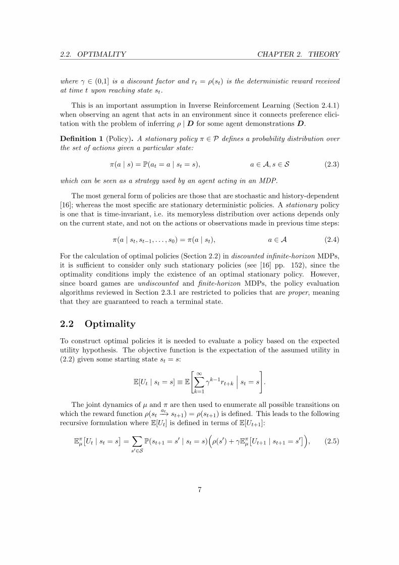
Example MDP
A deterministic mapping π : S → A from states to actions results in a single strategy-induced transition matrix T
π which defines the kernel of a regular Markov chain. Asan example of the dynamics of a simple MDP with 3 states and 2 actions, Figure 2.1shows a pictorial representation of the two different Markov chains induced by the two
1Markov process — A stochastic process which has the Markov property, i.e. being memoryless, s.t.transitions between states depend solely on the current state that the system is in.
2Sometimes more general definitions are used, such as the reward function ρ : S ×A×S → R definedon the space of all possible transitions st
at−→ st+1.
5
2.1. DECISION MAKING UNDER UNCERTAINTY CHAPTER 2. THEORY
strategies π1(·) = a1 and π2(·) = a2. In this example, T π1 and Tπ2 are given by:
Tπ1 =
1/2 1/2 0
0 1 0
1 0 0
T
π2 =
1 0 0
1/2 0 1/2
1/2 0 1/2
(2.1)
s.t. element (st,st+1) denotes the transition probabilities between those states. Thus,T
π for any particular strategy π is then a mixture of the two.
+10
-5 +1
1
1/2
1/2
1
+10
-5 +1
1/2 1/2
1/2
1/21
Figure 2.1: A pictorial representation of an MDP where arrows indicate transition prob-abilities for a1 (left) and a2 (right). Rewards are shown inside the nodes and are supposedto be identical in the two images.
2.1.2 Policies
To be able to formulate an optimal policy, i.e. an optimal strategy for an agent actingin an MDP, it is necessary to make assumptions regarding the objective function beingoptimised.
Since the preferences of an agent are indeed subjective, decision theory handles theproblem by formalising the notion of an agent’s utility as a function U : R → R, whereR can formally be seen as the set of all possible reward sequences of different lengths.It is then said that if an agent prefers a reward r1 to r2, then E
[U(r1)
]> E
[U(r2)
]; also
known as the expected utility hypothesis [14].Further, the following assumption is a common one to make, which is found in most
literature on MDPs [15].
Assumption 1 (Agent utility). The agent acts to maximize the discounted sum of future
rewards
Ut ,
∞∑
k=1
γk−1rt+k, (2.2)
6
2.2. OPTIMALITY CHAPTER 2. THEORY
where γ ∈ (0,1] is a discount factor and rt = ρ(st) is the deterministic reward received
at time t upon reaching state st.
This is an important assumption in Inverse Reinforcement Learning (Section 2.4.1)when observing an agent that acts in an environment since it connects preference elici-tation with the problem of inferring ρ |D for some agent demonstrations D.
Definition 1 (Policy). A stationary policy π ∈ P defines a probability distribution over
the set of actions given a particular state:
π(a | s) = P(at = a | st = s), a ∈ A, s ∈ S (2.3)
which can be seen as a strategy used by an agent acting in an MDP.
The most general form of policies are those that are stochastic and history-dependent[16]; whereas the most specific are stationary deterministic policies. A stationary policyis one that is time-invariant, i.e. its memoryless distribution over actions depends onlyon the current state, and not on the actions or observations made in previous time steps:
π(a | st, st−1, . . . , s0) = π(a | st), a ∈ A (2.4)
For the calculation of optimal policies (Section 2.2) in discounted infinite-horizon MDPs,it is sufficient to consider only such stationary policies (see [16] pp. 152), since theoptimality conditions imply the existence of an optimal stationary policy. However,since board games are undiscounted and finite-horizon MDPs, the policy evaluationalgorithms reviewed in Section 2.3.1 are restricted to policies that are proper, meaningthat they are guaranteed to reach a terminal state.
2.2 Optimality
To construct optimal policies it is needed to evaluate a policy based on the expectedutility hypothesis. The objective function is the expectation of the assumed utility in(2.2) given some starting state st = s:
E[Ut | st = s] ≡ E
[∞∑
k=1
γk−1rt+k
∣∣∣ st = s
].
The joint dynamics of µ and π are then used to enumerate all possible transitions onwhich the reward function ρ(st
at−→ st+1) = ρ(st+1) is defined. This leads to the followingrecursive formulation where E[Ut] is defined in terms of E[Ut+1]:
Eπµ
[Ut | st = s
]=
∑
s′∈S
P(st+1 = s′ | st = s)(ρ(s′) + γEπ
µ
[Ut+1 | st+1 = s′
]), (2.5)
7
2.2. OPTIMALITY CHAPTER 2. THEORY
where the indices µ and π indicate that the expectation is over the dynamics of the MDPst+1 | st ∼ τat and the actions of the policy at | st ∼ π s.t.
P(st+1 | st) =∑
a∈A
P(st+1 | st,at = a)P(at = a | st)
≡∑
a∈A
τa(st+1 | st)π(at = a | st).
This is a good time to introduce the value function which serves a more intuitivenotation:
V πµ (s) , E
πµ
[Ut | st = s
]
=∑
s′∈S
∑
a∈A
π(a | s)τa(s′ | s)
(ρ(s′) + γV π
µ (s′)), (2.6)
From here on, the subscript µ will be dropped whenever it is clear from context. Later,however, when the need arises to distinguish between the values in different tasks(MDPs), the only varying element will be ρ ∈ µ and the notation V π
ρ will be used
instead. An optimal policy π∗ has the property V π∗
= V ∗ where
V ∗(s) , maxa
{∑
s′∈S
Pa(s′ | s)
(ρ(s′) + γV ∗(s′)
)}, ∀s ∈ S (2.7)
Another common notation is the Q-value of a state-action pair (s,a), defined as theexpected utility conditioned on action a taken in state s:
Qπ(s,a) , E[U | s,a
](2.8)
= E[ρ(s′) | s,a
]+ γ
∑
s′∈S
τa(s′ | s)
∑
a′∈A
π(a′ | s)Q(s′,a′) (2.9)
=∑
s′∈S
τa(s′ | s)
(ρ(s′) + γV π(s′)
)(2.10)
and Q∗(s,a) , Qπ∗
(s,a), (2.11)
s.t. V ∗(s) ≡ maxa
{Q∗(s,a)
}(2.12)
2.2.1 Bellman Optimality Equations
The value of a policy in (2.6) and that of the optimal policy in (2.7) are the two equationsknown as the Bellman equation and Bellman optimality equation respectively [17], whichform the basis of the policy evalutation and value iteration algorithms. These algorithmsboth apply the respective equation as an update rule to all possible states until the valuesof all states no longer change.
Consider the MDP from the previous example in Figure 2.1 and assume an infinitehorizon and γ = 1
2 for simplicity, and focus on the left side induced by the policy π1(·) =a1. The value V
π1(s2) of the top right state denoted by s2 for this policy is the easiest to
8
2.3. TEMPORAL DIFFERENCE LEARNING CHAPTER 2. THEORY
calculate, since it is given by the geometric series V π1(s2) = 1× (ρ(s2) + γV π1(s2)) = 2.By backtracking to the top left state, denoted by s1, there is only one unknown variable(value) which can be solved by V π1(s1) = 1
2 × (−5 + γV π1(s2)) +12 × (1 + γV π1(s1)),
giving V π1(s1) = −2. Similarly, V π1(s3) = −6.At a more general note, Equation (2.6) forms a linear system of equations:
vπ = Tπr + γT πvπ, (2.13)
which has the solution given by the policy evaluation step:
vπ = (I − γT π)−1T
πr. (2.14)
In the case discussed above, the value function is vπ1 = (−2, 2,−6)⊤. In other words,given the policy π1 that only chooses action a1, the bottom state is not very good. Apolicy improvement step would update the policy similarly to Equation (2.7):
πn+1(s) = argmaxa
{∑
s′∈S
Pa(s′ | s)
(ρ(s′) + γVn(s
′))}
, ∀s ∈ S
⇔
πn+1 = argmaxπ
{T
π(r + γvn)},
(2.15)
where the subscript n denotes the iteration index. In this case, the updated policy wouldbe πn+1((s1, s2, s3)
⊤) = (a1, a1, a2)⊤, i.e. where the action changed only in s3 from a1
to a2, giving vπn+1 = (−2, 2, 83)⊤. The policy induced transition kernel T πn+1 is then
constructed by choosing rows 1,2 from Tπ1 and row 3 from T
π2 . In yet another andfinal iteration in the same manner, the algorithm would converge to the optimal policydenoted by π∗ = πn+2((s1, s2, s3)
⊤) = (a1, a2, a2)⊤, giving the optimal value function
v∗ = vπ∗
= (2, 83 ,83)
⊤. This concludes the example of the policy iteration algorithm.Policy iteration iteratively performs steps (2.14) and (2.15) until convergence, i.e.
until ‖vn − vn+1‖ ≤ ε (which is also implied when πn+1 = πn).Value iteration combines these steps such that the policy is not queried, but the
maximum over actions is taken in each iteration, see Algorithm 1.
2.3 Temporal Difference learning
Temporal Difference (TD) learning methods [12, 18] attempt to estimate the value func-tion V π(·) for a given policy π:
V π(st) = ρ(st+1) + γV π(st+1), (2.16)
given one or more finite sample trajectories of kind {st}Tt=1 generated by π, where sT is
a terminal state with a reward (outcome) ρ(sT ). They attempt to solve the (temporal)credit assignment problem inherent in problems with delayed rewards [9], such as boardgames where the reinforcement is usually delayed until the very last (terminal) states.
9
2.3. TEMPORAL DIFFERENCE LEARNING CHAPTER 2. THEORY
Algorithm 1: Value Iteration
Input: MDP µ Discount factor γ, Precision parameter εResult: Vector v s.t. vs = V ∗
µ (s), ∀s ∈ Sv0 ← 0n← 0repeat
n← n+ 1foreach s ∈ S do
vn(s)← maxa
{∑
s′∈S
τa(s′ | s)
(ρ(s′) + γvn−1(s
′))}
end
until ‖vn − vn−1‖ ≤ ε;return vn
The method attempts to match current estimates V (st) with (hopefully) more accuratebeliefs about the values for future states V (sk), k > t. This takes advantage of theassumption that subsequent values V (st), V (st+1), . . . are correlated.
A regular Monte Carlo (MC) learning method would approximate the value V (st)by generating a rollout3 sample Ut and applying the update rule:
V (st)← V (st) + α(Ut − V (st)
), (2.17)
where α is a step size parameter. Clearly, if the current prediction Vt matches the targetvalue E[Ut], the value function has been learned and only fluctuates depending on thestep size α. The issue with this method, however, is that a full trajectory needs to begenerated for every sample of Ut. TD-methods instead attempt to minimize the TD-error
between subsequent states by applying the update rule:
V (st)← V (st) + α(ρ(st+1) + γV (st+1)− V (st)
). (2.18)
The target instead becomes E[ρ(st+1)+γV (st+1)
], which, since V (st+1) is itself a current
estimate maintained by the algorithm, makes TD-learning a bootstrapping method.Algorithm 2 presents a version of this method which queries the policy in an on-line
fashion, updating the value function as the trajectory is being generated.For the coming section, it is instructive to use the state-action value notation Qπ(s,a)
and to briefly introduce on-policy and off-policy learning, for which two common exam-ples (among TD-methods) are Sarsa [12, 19] and Q-learning [20] respectively. Both ofthese methods attempt to learn an optimal value function, whereas the former of the twoworks nearly identically to Algorithm 2 apart from two modifications. First, to chooseactions at,at+1, . . . , Sarsa queries a policy πQπ that chooses its actions based on the
3Rollout - sample trajectory from a starting state following some policy π until a terminal state isreached, resulting in a sampled cumulative sum of returns Ut.
10
2.3. TEMPORAL DIFFERENCE LEARNING CHAPTER 2. THEORY
Algorithm 2: TD-learning of V π
Input: MDP µ, Policy π, Discount factor γ, Precision parameter εResult: Vector v s.t. vs ≈ V
πµ (s), ∀s ∈ S
v ← 0repeat
t← 0s0 ← starting stateδmax ← 0repeat
at ∼ π(· | st)st+1 ∼ τa(st)δ ← ρ(st+1) + γvst+1 − vstvst ← vst + αδδmax ← max
{|δ|, δmax
}
t← t+ 1until st is terminal ;
until δmax ≤ ε;return v
current belief over the state-action values Qπ. The convergence properties to Q∗ relyon the policy’s ability to balance between exploration and exploitation [12], and mostimportantly, that π is gradually tuned to be more greedy w.r.t. Qπ. The update is thendone on the these state-action values:
Qπst,at ← Qπ
st,at + α(ρ(st+1) + γQπ
st+1,at+1−Qπ
st,at
). (2.19)
In Q-learning, the difference is subtle; the definition of an off-policy method is that itdoes not learn the value function of the policy followed. In this case, the value functionlearned is still Q∗ but the only requirement on the policy is that all state-action pairsare visited and updated. The update is then given by:
Qst,at ← Qst,at + α(ρ(st+1) + γmax
aQst+1,a −Qst,at
). (2.20)
2.3.1 Least-squares methods
This section describes least-squares methods of approximating the value function of apolicy. This is the same task as the previously mentioned algorithms are solving, butthe solutions presented here are adapted to handle large state spaces.
Feature representation
From here on, the value functions will be approximated with feature representations ofthe state-action pairs, mainly so that large state spaces can be handled more efficiently.
11
2.3. TEMPORAL DIFFERENCE LEARNING CHAPTER 2. THEORY
For the state-action value function used in this section, the approximation is defined bythe linear combination
Q(s,a) , φ(s,a)⊤w, φ(s,a),w ∈ Rk, (2.21)
or by the more compact notation
q = Φw, Φ ∈ R|S||A|×k,w ∈ R
k. (2.22)
Where each feature vector, given by the function φ : S × A → Rk, is comprised of k
different, generally nonlinear, functions of the state-action pairs. The symbol q will beused to denote any value function, and q to denote a value function that lies in thesubspace spanned by Φ.
Bellman residual minimisation
This section acts as a bridge to the explanation of the LSTDQ algorithm presentedin the next section, and it partly follows the presentation made by its authors in [21].It is a natural extension to solving the linear system for the value function when it isapproximated by a linear combination of features.
Recall the Bellman equation for Qπ(s,a) in Equation (2.9) and note that it has thelinear system representation
qπ = r + γT πqπ, (2.23)
where q, r ∈ R|S||A|, r(s,a) = E
[ρ(s′) | s,a
]and T
π ∈ R|S||A|×|S||A|. In this context, T π
is the policy induced transition kernel of a Markov chain with transitions of the kind(s,a) → (s′,a′) with probability T π
(s,a),(s′,a′). The summation over pairs (s′,a′) in (2.9),
where the expectation is given a state-action pair (s,a), can be seen as T πq = T Ππqπ
where T(s,a),s′ = τa(s′ | s) and Πs′,(s′,a′) = π(a′ | s′).
The right hand side of the linear system in (2.23) is often defined as the Bellman
operator Lπ applied to the left hand side. In other words, a shorthand for the linearsystem is qπ = Lπq
π, and in an iterative policy evaluation scheme the updates areqn+1 ← Lπqn.
Replacing qπ with Φwπ gives an overconstrained system (since k < |S||A|) with theleast-squares solution:
wπ =((Φ− γT πΦ)⊤(Φ− γT πΦ)⊤
)−1(Φ− γT πΦ)⊤r (2.24)
This is a natural approach that mimics everything that we have learned so far; the onlydifference being that a linear feature approximation makes the system overconstrained.The interesting property to remember, however, is that the solution minimises the Bell-
man residual, i.e. the L2 distance taken by Lπ when applied to Φw. This helps inunderstanding why LSTDQ takes a different approach; and why that approach may bebetter.
12
2.3. TEMPORAL DIFFERENCE LEARNING CHAPTER 2. THEORY
Note that the Bellman operator applied to Φw, a point in the feature plane, gives aresulting point that is generally outside that plane. The Bellman residual minimisation
above minimises this distance, but LSTDQ attempts to find a solution such that, whenthe Bellman operator is applied to it, the resulting vector is still in the feature plane:
q ≈ Lπq. (2.25)
The equation can then be expressed as follows. The value function should be invariantto the combined operation of applying the Bellman operator and then projecting theresult onto the feature plane:
qπ = PΦLπqπ, (2.26)
where the orthogonal projection PΦ onto the subspace spanned by Φ is given byΦ(Φ⊤Φ)−1Φ⊤ (cf. [22] pp. 430 eq. (5.13.3)). The solution to this system is
wπ =(Φ⊤
(Φ− γT πΦ
))−1Φ⊤r, (2.27)
whose derivation can be found in [21] and is left out here for brevity. This method triesto find the point in the feature plane closest to the true value function. If the real valuefunction is actually inside the feature plane, the two different methods give the sameresult.
The algorithm proceeds as follows. Given some data D ={(si, ai, s
′i, ri)
}L
i=1of
transitions, let f : |S||A| → R be a probability distribution over the state-action pairs,s.t. fD is the true distribution of D, and let ∆f be a diagonal matrix with elementsf(s,a). Then the LSTDQ algorithm builds empirical estimates of
A = Φ⊤∆fD
(Φ− γT πΦ
), and (2.28)
b = Φ⊤∆fDr (2.29)
given by
A =1
L
L∑
i=1
φ(si,ai)(φ(si,ai)− γφ(s
′i, π(s
′i))
)⊤, and (2.30)
b =1
L
L∑
i=1
φ(si,ai)ri (2.31)
s.t. the solution is given by wπ = A−1
b. In the limit of L → ∞, this gives the truesolution biased by the distribution of the data fD. LSTDQ is summarised in Algorithm3.
13
2.3. TEMPORAL DIFFERENCE LEARNING CHAPTER 2. THEORY
Algorithm 3: LSTDQ
Input: Data D, Basis functions φ, Discount factor γ, Policy πResult: Vector w s.t. Qπ(s,a) ≈ φ(s,a)⊤wA← 0b← 0foreach (s,a,s′,r) ∈D do
A← A+ φ(s,a)(φ(s,a)− γφ(s′,π(s′))
)⊤
b← b+ φ(s,a)rend
return wπ = A−1
b
Least-squares Policy Iteration (LSPI)
LSTDQ is an extension of LSTD from previous work in [23, 24] which is based on statevalues V . The issue with LSTD, as argued by [21], is that it cannot be used for actionselection without a model of the underlying process. For instance, had the model T ∈ µbeen given, together with a value function V a policy π with the property V ≡ V π
can always be constructed as π(s) = argmaxa{∑
s′∈S τa(s′ | s)
(ρ(s′) + γV (s′)
)}. This
concern is relevant in board games, where the actions made by the opponent are anunknown stochastic part of the model.
When state-action values Q are given, the policy can be constructed directly byπ(s) = argmaxa
{Q(s,a)
}. To demonstrate the benefits, the authors also suggest a
model-free policy iteration algorithm for finding an optimal4 policy by using LSTDQ. Thealgorithm is named Least Squares Policy Iteration (LSPI) and is presented in Algorithm4.
4The performance of the policy π returned by LSPI is bounded by ‖Qπ −Q∗‖∞ ≤ 2γε(1−γ)2
, details
given in [21].
14
2.4. LEARNING FROM DEMONSTRATIONS CHAPTER 2. THEORY
2.4 Learning from demonstrations
A value function roughly states how to accomplish a task, since it directly defines adeterministic policy. For example, in large and complex environments the goal may beto reach a specific terminal state, such as escaping a maze, retrieving an item or winninga board game. The value function then measures the proximity of such a goal. Statinga value function manually is thus a difficult task subject to bias in the resulting policy.Algorithms learning the value function directly also need to worry about generalisingwell to unseen states.
The reward function is a natural abstraction that instead states what to accomplish,e.g. by assigning a numerical reward of +1 to goal states and 0 to all others. This allowsthe algorithms discussed so far to find optimal value functions and optimal policieswith no bias. However, for long and complex tasks in large environments, they becomeinefficient unless a proper set of subgoals can be defined. If certain subgoals do indeedsignify progress towards the end goal, they could be assigned positive rewards; butidentifying such subtasks is a difficult problem.
Inverse reinforcement learning [25, 26] is concerned with inferring the inherent pref-erences of a demonstrator or expert from its observed interactions with an environment.Constructing good reward functions thus becomes an inference task. This section ex-plains IRL techniques for construction of reward functions through the use of unlabeleddata, which is the common approach since data where the goals have been labeled ismuch less common.
When multiple experts act in the same environment, their individual subgoals may bedifferent and the method explained here infer them in a multiple task setting. The mainfocus is on the multitask Bayesian approach proposed in [7]; an extension of its singletask counterpart in [1]. This is reviewed in the next section. Some previous multitaskBayesian approaches include [27, 28, 29] but are not covered here.
When dealing with IRL it is instructive to separate the MDP tuple into the partsµ = (ν, ρ, γ), where ν = (S,A,T ) is a controlled Markov process (CMP) defining thedynamics of the game/system. In this framework, we will distinguish between M dif-ferent tasks {µm = (ν, ρm, γ)}
Mm=1 so that the only varying element between tasks is the
reward function. For each task m, there is a set of demonstrations dm, s.t. the completedataset is denoted by D = {dm}
Mm=1. The corresponding sets of (unknown) reward
functions and policies are denoted by ρ = {ρm}Mm=1 and π = {πm}
Mm=1 respectively.
The following model employs a hierarchical Bayesian approach with a hyperprior η onthe joint reward-policy priors φ. Since η is defined on the joint reward-policy distribution
function space, rather than on the parameters of some fixed functions’ parameters, itbecomes the only parameter to the model in a very general sense.
As the first of two examples demonstrated in [1], if η is chosen as the distribution ona product prior φ on reward functions and policy Softmax temperatures (i.e. noise levels,see Section 3.3), it then jointly determines unique policies for which the likelihood of the
15
2.4. LEARNING FROM DEMONSTRATIONS CHAPTER 2. THEORY
data is well defined. This is clear because a sampled reward function ρ gives rise to anoptimal value function Q∗
ρ which induces a policy π that follows Q∗ρ according to a well
defined probability with noise. From here on, the notation Qρ , Qµ, where µ = (ν,ρ,γ),will be used to emphasis the dependency on ρ.
The second formulation, to be used here, lets η be a distribution on priors φ on policy
functions and on the optimality of the policies, leading to an implicit distribution onreward functions conditional on policies. The posterior probability of a reward functioncan then be calculated as the marginal over a set of sampled posterior policies. This isthe heart of the algorithm, to be made more clear here.
Model
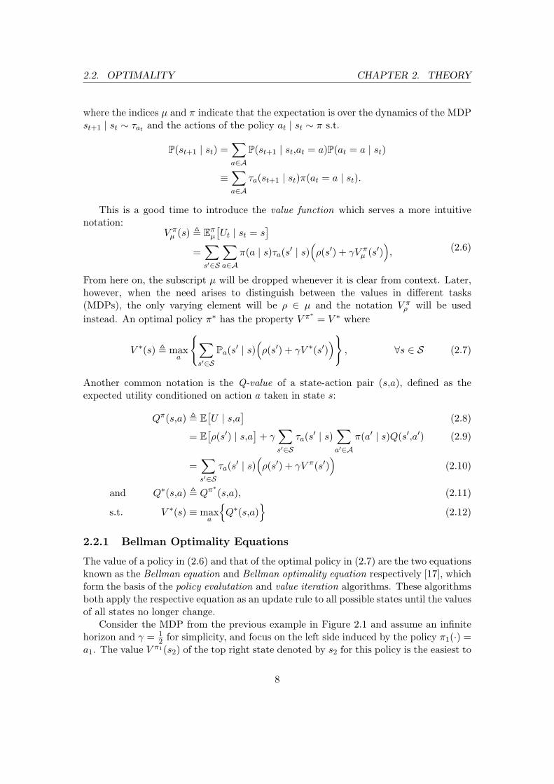
The joint reward prior ψ and policy prior ξ, denoted by φ, is sampled from the hyperpriorη. The notation φ will not be used very much, but it is connected to the individual priorsin the sense that φ is a probability measure on the reward-policy product space R× Paccording to φ(R,P | ν) ,
∫R ξ(P | ν)dψ(ρ | ν) for R ⊂ R and P ⊂ P. ψ(ρm = ρ | ν)
denotes the prior probability that the m:th reward function is ρ, and ξ(πm = π | ν)denotes the prior probability that them:th policy is π. The dependencies on ν will be leftout for clarity, since it stays constant throughout the different tasks. The correspondingposteriors are denoted by ψ(· |D) and ξ(· |D). The model is shown in Figure 2.2.
η φ ρm
πm
dm
M
Figure 2.2: Graphical model of the reward-policy priors. Darker color indicates observ-ables. Here, ρm,πm is sampled jointly from φ, indicated by the undirected edge betweenthem. The data dm is generated by the m:th demonstrator’s policy πm.
Derivation
The purpose of Bayesian IRL is to calculate the posterior probability ψ(· |D) on rewardfunctions. As mentioned, this model does so by approximating the marginal over policyposteriors
ψ(ρ |D) =∑
π∈P
ψ(ρ | π)ξ(π |D) (2.32)
by sampling from ξ(· | D). The policy posterior is simple to calculate if, for instance,ξ ∼ Dir(α) is chosen. Thus, the main goal is to find a way to express and approximateψ(ρ | π).
16
2.4. LEARNING FROM DEMONSTRATIONS CHAPTER 2. THEORY
Let the loss of policy π w.r.t. reward function ρ be defined as
ℓρ(π) , maxs
∥∥V ∗ρ (s)− V
πρ (s)
∥∥. (2.33)
A policy is said to be ε-optimal w.r.t. ρ if ℓρ(π) < ε. Let the prior probability thatℓρ(π) = ε be given by β(ε | π) for any ρ, and assume β(ε | π) = β(ε)5. Then β([0,ε])is the prior probability that the policy is ε-optimal. This opens up the possibility tocalculate ψ(ρ | π) via
ψ(ρ | π) =
∫ ∞
0ψ(ρ | ε,π)dβ(ε), (2.34)
where ψ(ρ | ε,π) can be interpreted as a prior probability measure on R given that π isε-optimal. The marginal posterior (2.32) can then be written as
ψ(ρ |D) =∑
π∈P
(∫ ∞
0ψ(ρ | ε,π)dβ(ε)
)ξ(π |D). (2.35)
The next task is then to find a motivated expression for ψ(ρ | ε,π). Let Rπε ,
{ρ ∈ R : ℓρ(π) < ε} be the set of reward functions for which π is ε-optimal. Then thefollowing definition is motivated in [1] by using a counting measure on R:
ψ(ρ | ε,π) ,✶Rπ
ε(ρ)
|Rπε |
, (2.36)
which can be seen as an unnormalised prior on reward functions.
Assuming that some finite setR is given, and thatK policies π(1), . . . ,π(k), . . . ,π(K) iid∼
ξ(· | D) are sampled from the posterior, a loss matrix L ∈ RK×|R| can be constructed
from (2.33). One final observation remains for (2.32) to be approximated. Let (εi)K×|R|i=1
be a monotonically increasing sequence of the elements of L. Then ψ(ρ | ε,π) = ψ(ρ |ε′,π) for any ε,ε′ ∈ [εi,εi+1], and the approximation is finally given by:
ψ(ρ |D) =K∑
k=1
K|R|∑
i=1
ψ(ρ | ǫi,π(k))β([ǫi,ǫi+1]) (2.37)
=
K∑
k=1
K|R|∑
i=1
✶Rπ(k)
εi
(ρ)
|Rπ(k)
εi |β([ǫi,ǫi+1]). (2.38)
Algorithm
The end result is a Monte Carlo approximation scheme shown in Algorithm 5; K beingthe number of MC samples. Here, the hyperprior generates ξ (i.e. α if ξ ∼ Dir(α)) anda parameter for the chosen form of the optimality prior β.
5This is not to be confused with the Beta distribution. In fact, later, β is chosen to be the exponentialdistribution.
17
2.4. LEARNING FROM DEMONSTRATIONS CHAPTER 2. THEORY
Algorithm 5: Bayesian Multitask IRL - Monte Carlo approximation
Input: Reward functions Rfor k = 1, . . . ,K do
(ξ(k),β(k)) ∼ ηfor m = 1, . . . ,M do
π(k)m ∼ ξ(· | dm)
end
end
Calculate ψ(· | dm) from (2.37) and{π(k)m
}K
k=1for all m
18
3
Model
This chapter explains the choices required to implement the Bayesian multitask InverseReinforcement Learning algorithm (BMTIRL) (Algorithm 5).
Since the algorithm calculates a probability distribution on the reward space R, theexpected reward function
ρm ,∑
ρ∈R
ψ(ρ | dm)ρ (3.1)
and its corresponding optimal policy π∗m , π∗ρm , where π∗ρ , π∗µ=(ν,ρ,γ), will be used
to denote the outputs of the algorithm. The true m:th reward function denoted by ρmrepresents them:th expert’s intrinsic goals, and technically means that the agent believesthat it is interacting with the environment µm = (ν,ρm,γ) in which it is not necessarilyoptimal. All experts are however acting in the same real environment µ = (ν,ρ,γ) and itis assumed that each ρm is drawn from some distribution with mean ρ. To approximateρ, the combined reward function across all experts will be used and is denoted by
ρ ,1
M
M∑
m=1
ρm, (3.2)
with the corresponding optimal policy denoted by π∗ , π∗ρ.Section 3.5 discusses how to construct R when there exists some approximation of
the optimal value function. The hope is that the value V ∗ρ of the optimal policy inferred
from all experts is somehow closer to the true optimal value function V ∗ρ than any (or
most) of the individual value functions V ∗ρm
. This may be due to the fact that differentexperts contribute to different parts of the feature vector that is used to approximate V .Figure 3.1 shows a schematic representation of this assumption.
19
3.1. FEATURES CHAPTER 3. MODEL
¶m2
VΡ
*
VΡ`*
VΡm2
*
VΡ`
m2
*
VΡm2
Πm2
VΡm1
*
VΡ`
m1
*
VΡm1
Πm1
¶m1
VΡ`
m2
Π dm2
VΡ`
m1
Π dm1
Figure 3.1: A schematic representation of the assumed relationship between the valuefunctions for the different environments considered in the inference process. In the centerof the figure lies the true value function V ∗
ρ of optimal play, and close to it are two differentexperts’ intended value functions Vρm1,2
. Implied by the colored areas around the experts’
actual values Vπm1,2
ρm1,2are all possible value functions from pairs of sampled policies and
reward functions. The approximated optimal value V ∗
ρ derived from ρm1,2is assumed to lie
close to the true optimal value V ∗
ρ .
3.1 Features
Although features for state-action pairs have been mentioned, a definition has not beenchosen yet. In many board games an action implies a local interaction within a subregionof the board. It is thus a natural choice for a state-action feature vector to be composedof features from this region only. However, for simplicity, the choice made here is to definethe state-action feature vector as the expected vector given by transition probabilitiesfor action a in state s:
φ(s,a) ,∑
s′∈S
τa(s′ | s)φ(s), (3.3)
where φ(s) is a set of nonlinear functions of the state s independent of the previousaction. This method of averaging feature vectors has some convenient properties, asshall be seen later. The chosen features for the different environments are explained inSection 3.2.
3.1.1 Reward function feature representation
Recall that the rewards are chosen as a function of the state transitioned to, althoughin the most general case they may be a function of all parameters from the transition
20
3.2. ENVIRONMENTS CHAPTER 3. MODEL
(such as the action). Regarding the argument made in Section 3.1 above, this wouldhave allowed for the combination of state-action features and rewards defined on them.For the applications discussed here, however, it will be sufficient to continue with thecurrent convention and to choose the definition:
ρw(s) , φ(s)⊤w. (3.4)
3.2 Environments
This section explains the MDP environments that will be examined.
3.2.1 Random MDP
The feature vector of a state in the Random MDP state space is chosen to have the samelength as the feature space |S| and to have the following one-hot encoding representation:
φi(s) ,
1 if i = s
0 otherwise(3.5)
Note that, together with (3.3), this definition leads to the property that φs′(s,a) ≡ τa(s′ |
s), i.e. that the state-action feature vector is a list of transition probabilities for the givenaction.
The transition kernel T will be sampled so that the τ ∈ T are given by τ a(·, s)iid∼
Dir(α) for all (a,s) ∈ A× S.The reward function is sampled according to Equation (3.4) and w ∼ Dir(α). Note
that, together with (3.3) and (3.5), this implies that ρw(s) ≡ ws.
3.2.2 Tic-tac-toe
Tic-tac-toe is the famous game where two players, referred to as X and O, take turnsplacing symbols on a board of size 3 × 3 until either one player has three symbols in arow (in any orientation) or the board is filled without a winner (a tie).
Tic-tac-toe is chosen for its state space being large enough for approximation byvalue iteration to be impractical, but small enough for having a known optimal policyand natural features. Although the state space can in fact be reduced to manageablesizes by considering equivalent reflections and rotations of the board, this is not thepurpose of the work and will not be done here. It will be handled as though the statespace is indeed of size 39 = 19683, i.e. by representing the state by an integer in therange [0,19683], although most of those states are not even legal positions. The numberof legal actions varies between 0 to 9 depending on the number of occupied locations ofthe board (of size 3× 3).
To make the translation to an MDP simpler, the dynamics will have player X in focus,so that every transition leads to a state where it is X’s turn to play unless the game ends.
21
3.3. GENERATION OF DEMONSTRATIONS CHAPTER 3. MODEL
The opponent is the random player, so that the transition probabilities given a move byX are uniformly distributed by the available remaining moves for O.
An optimal strategy is given by a heuristic set of rules in [30], which will be referredto as the programmatic optimal policy.1
Features
The feature vector for a state in the Tic-tac-toe environment is chosen to be a subset ofthe features discussed in [31], namely, for each player X and O: the number of singlets(lines in any orientation with exactly one symbol), doublets (like singlets but exactly two
identical symbols), triplets (three identical symbols in a row), crosspoints (the numberof empty points that belong to at least two singlets), corners (the number of occupiedcorners), and finally a center occupation feature with value in {−1,0,1} for O, empty andX respectively. Apart from these features, an extra fork feature is added, defined as thenumber of distinct doublets - 1. Apart from the center occupation feature, all featuresare defined for both players, which makes a total of k = 13 features.
The choice of adding the fork feature was made so that the programmatic optimalpolicy could be implemented by the use of features and one step lookahead alone.
Rewards
True rewards are given in the terminal states (win or tie) as {−1,0,1} for a loss, tie andwin respectively. Let x be the index of the triplets feature for X and o the correspondingindex for O, then the true reward function ρw is defined by
wi =
1 if i = x,
−1 if i = o,
0 otherwise.
(3.6)
Naturally, when a reward function ρ ∈ R during inference in BMTIRL is considered, itwill be used instead of (3.6).
3.3 Generation of demonstrations
Recall that an optimal policy given a value function Q(s,a) is based on the maximisationπ∗Q(s) , argmaxa{Q(s,a)}. A common alternative [13] that makes the policy (infinitely)differentiable is to define a Softmax policy according to
πSoftmax(c)Q (a | s) ,
eQ(s,a)/c
∑a′∈A eQ(s,a′)/c
, (3.7)
1As is also referenced and reviewed in http://en.wikipedia.org/wiki/Tic-tac-toe#Strategy; ac-cessed at 2014-05-10.
where c is a temperature parameter with the properties limc→0 πSoftmax(c)Q = π∗Q and
that limc→∞ πSoftmax(c)Q is the uniformly random policy. It will be used here to generate
demonstrations so that the noise level can be controlled. No real data from human playwill be used.
Each expert m generates a dataset dm (see Figure 2.2) consisting of N independenttrajectories of total lengths T1, . . . ,Tn, . . . ,TN :
dm =
{((s
(n)t ,a
(n)t )
)Tn
t=1
}N
n=1
. (3.8)
Each trajectory n starts in a state s0 drawn from some initial state distribution, actions
are sampled by at ∼ πSoftmax(c)Q (· | st) and states by st+1 ∼ τat(· | st) until st = sTn .
The termination may be chosen either by setting a fixed demonstration length or by justfollowing the policy until a terminal state is reached2.
3.4 Policy space
The approximation of the posterior reward distribution in Equation (2.37) relies on
samples π(k)m from πm | dm, where the policy prior is chosen s.t. πm(· | s) ∼ Dir(α) for
all s ∈ S.For a state s, the updates of the Dirichlet parameters α
(s)a for each action a is given
by simply adding the count of the number of times that (s,a) was observed in dm:
α(s)a = α(s)
a +N∑
n=1
Tn∑
t=1
✶
{s(n)t = s ∧ a
(n)t = a : (s
(n)t , a
(n)t ) ∈ dm
}, (3.9)
which applies for all (s,a) ∈ S ×A. At a first glance, this requires the enumeration of all
parameters α(s)a , which would be intractable since this work focuses on too large state
spaces. However, it is still possible for a lazy3 representation in the following sense. Forevery expert m, the posterior is stored as counts of observed state-action pairs in dm,
and for every sampled policy π(k)m , a multinomial is sampled and stored only once for
every s upon the querying of π(k)m (· | s).
3.4.1 Loss calculation
The loss calculation ℓρ(π) in (2.33) amounts to estimating V πρ and V ∗
ρ for all states, butsince all states cannot be enumerated, a subset S ⊂ S has to be used instead. Also, dueto that the posterior policy will have updated parameters only in observed states, thismotivates the choice of using S = {s : s ∈ dm} for each expert m.
2This assumes that policy is proper and is guaranteed to reach a terminal state, which holds triviallyfor the MDPs focused on here.
3Lazy initialisation — An object is not calculated before it is requested.
23
3.5. REWARD FUNCTION SPACE CHAPTER 3. MODEL
To actually estimate V πρ , LSTDQ (Algorithm 3) is used to get a vector of weights
w for which Qπρ ≈ φ(s,a)⊤w. Similarly, LSPI (Algorithm 4) is used to retrieve π∗ρ and
Q∗ρ. As LSTDQ relies on sampled transitions from some distribution (where the only
requirement is that the distribution visits all states), a completely random policy will beused to generate the LSTDQ-specific demonstrations for the random MDP.
3.5 Reward function space
This section connects the assumed value function space in Figure 3.1 with the generationof the reward space R. If an approximation of the optimal value function exists, theexperts’ intended value functions should also be close. Using a Gaussian approximationon state-action values, the distribution on the reward space can be solved for and thediscrete reward space R can be sampled.
In Equation (2.23), the linear system qπ = r + γT πqπ was based on Equation (2.9)where r(s,a) = E[ρ(s′) | s,a]. Using definitions (3.4) and (3.3) for the reward function
and state-action feature function respectively results in the equivalences r(s,a) , E[ρ(s′) |
s,a] ≡ φ(s,a)⊤w and r ≡ Φw, where Φ ∈ R|S||A|×k as in Section 2.3.1.4
Let r = q − γT πq denote the target values in a linear system r = Φw, so that itsleast-squares soluton is w = (Φ⊤Φ)−1Φr. Now assume that there exists some multi-variate normal approximation q of q with known correlations. With assumpions on thegame dynamics, this induces a transformed distribution for r denoted by µr,Σr.
This is different from regular Bayesian linear regression since, there, it is assumedthat every single target value ri has some unknown univariate i.i.d. noise εi ∼ N (0,σ2)added to it. In the above context, (µr,Σr) is already given and the problem is tocalculate (µw,Σw). The solution is calculated in [32] where the following expressionsare given by (14.11) and (14.12) in the cited work:
µw = (Φ⊤Σ−1r Φ)−1Φ⊤Σ−1
r µr, (3.10)
Σw = (Φ⊤Σ−1r Φ)−1. (3.11)
Each reward function ρi ∈ R, where ρi(s) = φ(s)⊤wi, is thus sampled according to:
wiiid∼ N (µw,Σw), (3.12)
which is equivalent to the slower procedure of — for every sample i — first sampling aset of values q ∈ R
|S||A| for some S ⊂ S, and then solving the linear system mentionedabove.
One limitation of BMTIRL is that it has to operate on a finite reward space R, whichmakes generating it an important task. The above procedure motivates why it can besampled using random playouts. In fact, in a message passing framework employed in
4Take careful note, however, that the weight vector w used in ρw is not the same as the one usedin Section 2.3.1 for value functions. Throughout this chapter, w is used only to describe the rewardfunction, hence a minimal risk for confusion.
24
3.5. REWARD FUNCTION SPACE CHAPTER 3. MODEL
[33], they motivate that only one random playout is necessary under the assumption thatterminal states with similar outcomes are clustered. The same approach will be usedhere to build estimates of the values.
25
4
Experiments
The general setup of the experiments are as follows.Given an increasing amount of data from each expert, the quality of the inference
was examined. In particular, the model (3.1) assumes that each expert m may havea different distribution on reward functions, and it does not know whether the expertsact in the same or similar environments (same or different ρm). Thus, convergence isshown for all experiments by measuring the loss ℓρm(π
∗m) of the m:th inferred optimal
policy (that is optimal w.r.t. the estimated reward function for each individual expertρm), evaluated in the m:th true environment given by ρm. When all experts use thesame reward function, this simplifies somewhat to the single task setting where the truereward function ρm = ρ will be chosen for all experts. The convergence measure is then(equivalently) ℓρ(π
∗m).
The performance is shown by measuring the loss ℓρ(π∗) of the policy π∗ (that is
optimal w.r.t. the inferred expected reward function ρ from (3.2)), evaluated in thetrue environment given by ρ. Note the similarity to the convergence measure in theprevious paragraph, and that in the single task setting the convergence and performanceare measured in the same space and can be viewed together, whereas in the multitasksetting these spaces are different and are viewed side by side.
4.1 Random MDP
The first experiment was to evaluate the algorithm a small randomly constructed MDPwith 20 states and 5 actions available in each state. Each transition probability vector
was sampled according to τa(· | s)iid∼ Dir(α = 1.0), ∀a ∈ A, and the true reward function
ρw was sampled by w ∼ Dir(α = 1.0). The set of proposal reward functions consistedof |R| = 20 i.i.d. samples from the same distribution as the true reward function. Theoptimality prior β was set to the exponential distribution with parameter λ = 10.0,which roughly sets a cumulative probability to a loss < 0.05 to approximately 40%. A
26
4.1. RANDOM MDP CHAPTER 4. EXPERIMENTS
ææ
æææ
æ
æ
æ
ææ
æ
à
ààà
à
à
àà
à
à à
ì
ì
ì
ìì
ì
ì
ì ì
ì ì
ò
ò
òò
ò
òò ò
ò ò
ò
ôô
ô
ô
ô
ô ô ô
ô ô
ô
æææ
ææ
æ
æ
æ
æ æ æ
0 500 1000 1500 2000ÈdmÈ0.00
0.05
0.10
0.15
{
æ {ΡHΠ`*L
æ {ΡHΠ`
1*L
à {ΡHΠ`
2*L
ì {ΡHΠ`
3*L
ò {ΡHΠ`
4*L
ô {ΡHΠ`
5*L
{ΡHΠ1L
{ΡHΠ2L
{ΡHΠ3L
{ΡHΠ4L
{ΡHΠ5L
(a) Losses of policies derived from inferred reward functions,where the policy derived from the average reward function isshown in dashed, blue.
a1
a2
a3
a4
a5
0.0 0.2 0.4 0.6 0.8 1.0
ΠHa È s5, DL
Expert 1 H~optimalL
Expert 5 H~randomL
(b) The posterior actionprobability for two differentexperts in state s5.
Figure 4.1: Single task convergence (a) of random MDP with 20 states and 5 actions, 5experts, γ = 0.90, K = 30 and |R| = 20. The choice of parameters makes the first expertnearly optimal and the last expert close to random as shown in in (b), due to Softmax actionprobabilities ∝ eQ(s,a)/c depending implicitly on the MDP parameters via the magnitudesof the value function.
discounting of γ = 0.9 was used.The first experiment examined the single task setting (ρm = ρ, ∀m) for 5 differ-
ent experts by setting the m:th expert’s Softmax temperature to cm = {0.001, 0.005,0.01, 0.015, 0.02}m. The experiment was repeated many times, and the results presentedin Figure 4.1 were representative. Increasing the size of the reward function space by20→ 60 gave improved results shown in Figure 4.2. In another experiment not reportedhere, the number was increased even further to 120, without any difference in results.
The multitask setting and the hypothesised relationship between value functions(Figure 3.1) were examined by perturbing the weight vector of the reward function ofeach expert by adding i.i.d. Gaussian noise with variance σ2 = 4.0 to each element,i.e. ρ = ρw, ρm = ρwm and wm ∼ N (w, 4.0). This value was chosen so that theperformance ℓρ(πm) of the experts’ policies πm (which are optimal w.r.t. ρm) would besignifinantly different than those of π∗ρ. The results presented in Figure 4.3 show that itis now possible to achieve a higher performance (lower loss) in comparison to those ofthe individual experts.
27
4.1. RANDOM MDP CHAPTER 4. EXPERIMENTS
æ
æ
æ
æ
æ
æ
æ æ æ æ æ
à
à
à
à
à
à à àà
à
à
ì
ìì
ì
ì ì
ì ì
ì
ì ì
ò
ò
ò
ò
ò
òò
ò
òò
ò
ô
ôô
ô
ô
ô
ô ô
ôô
ô
æ
æ
æ
æ
æ
æ
æ
æ
æ
æ æ
0 500 1000 1500 2000ÈdmÈ0.00
0.05
0.10
0.15
{
æ {ΡHΠ`*L
æ {ΡHΠ`
1*L
à {ΡHΠ`
2*L
ì {ΡHΠ`
3*L
ò {ΡHΠ`
4*L
ô {ΡHΠ`
5*L
{ΡHΠ1L
{ΡHΠ2L
{ΡHΠ3L
{ΡHΠ4L
{ΡHΠ5L
Figure 4.2: Random MDP with 20 states and 5 actions, 5 experts, γ = 0.90. The numberof reward functions is increased to |R| = 60, leading to lower losses reached.
æ
æ
ææ
æ
æ
æ ææ
æ
à
à
à
à
à
à
à à
à à
ì
ì
ì
ì
ì
ì
ìì
ì ì
ò
ò
òò
ò òò ò ò ò
ô
ô
ô
ô
ô
ô
ô ô ô ô
0 200 400 600 800 1000ÈdmÈ0
2
4
6
8
10
12
14{
æ {Ρ1HΠ`
1*L
à {Ρ2HΠ`
2*L
ì {Ρ3HΠ`
3*L
ò {Ρ4HΠ`
4*L
ô {Ρ5HΠ`
5*L
(a) Multitask convergence of losses.
æ
æ
ææ
æ æ
ææ
æ æ
0 200 400 600 800 1000ÈdmÈ0.14
0.16
0.18
0.20
0.22
0.24
0.26{
{ΡHΠ1L
{ΡHΠ2L
{ΡHΠ3L
{ΡHΠ4L
{ΡHΠ5L
æ {ΡHΠ`*L
(b) Multitask optimal policy π∗ performance intrue MDP compared to each expert.
Figure 4.3: Inference in the multitask setting where each expert has its own reward functionρwm
where wm ∼ N (w,4.0) and ρw is the true reward function. Parameters are K =10,|R| = 20,γ = 0.90 and all expert temperatures are set to 0.001.
28
4.2. TIC-TAC-TOE CHAPTER 4. EXPERIMENTS
Feature Prog. LSPI
Singlets X 0.151 0.190
Doublets X 0.212 0.306
Triplets X 0.879 0.884
Crosspoints X 0.004 0.009
Corners X 0.072 0.068
Forks X 0.153 0.280
Singlets O 0.186 0.370
Doublets O -0.063 -0.040
Triplets O -1.352 -1.518
Crosspoints O -0.258 -0.428
Corners O 0.100 0.099
Forks O -0.921 -1.434
Center occupation 0.030 0.013
Table 4.1: Weights found by evaluating the programmatic optimal policy (Prog.) usingLSTDQ, and those found by letting LSPI converge to an optimal policy from initial weightsw0 = 0.
4.2 Tic-tac-toe
The second experiment involved evaluating the multitask setting of the algorithm in theTic-tac-toe domain. First it was asserted that the programmatic optimal policy and thepolicy returned by LSPI had similar weights in their resulting value function. A numberof 5000 random playouts were generated as data for LSTDQ. This gave the weightspresented in Table 4.1. Some discrepancy does exist, but no further analysis was madeas to why. Both policies have roughly the same win rate against the random policy, buttheir strategies may be different.
Each reward function was sampled by first sampling a set of state-action values andthen solving the linear system given by those values, as explained in Section 3.5. Thestate-action values were sampled for every (s,a) ∈ X where X was the demonstrationsfrom 10 completely random playouts. To approximate the value of each (s,a) ∈ X, theterminal reward from 1 random playout was used. A number of R = 60 reward functionswere sampled this way.
The experts were then defined as Softmax policies similar to the previous exper-iments, with low to zero noise for easier observation of results. The experts’ valuefunctions were derived from an approximative reward function sampled according to theabove mentioned procedure (for a larger set of size |X| = 200), but where some weights
29
4.2. TIC-TAC-TOE CHAPTER 4. EXPERIMENTS
Feature Expert 1 Expert 2 Expert 3
Singlets X 1
Doublets X 1
Triplets X
Crosspoints X 1
Corners X 1 1
Forks X 1
Singlets O 1
Doublets O 1
Triplets O
Crosspoints O 1
Corners O 1 1
Forks O 1
Center occupation 1 1 1
Table 4.2: Factors of the reward weightsw used for each expert’s individual reward functionρw. The base reward function was a random sample using the procedure described in thetext. This method represents missing knowledge where the weights are 0 (empty tableelements).
were set to 0 to simulate lack of information processing capabilities. For instance, if theweight for ”Triplets X” were set to 0, the expert would not know how to win, but playoptimally up until the last move (and then possibly win by pure chance). The purposewas to construct experts whose scoring were not too high, and the feature weights werechosen arbitrarily to achieve this. The factors of the weights per expert’s reward functionis presented in Table 4.2.
The expert’s demonstrations dm were used as samples for the LSTDQ policy evalu-ation step as explained in Section 3.4.
The convergence of the multitask experiment is presented in Figure 4.4. The perfor-mance results presented in Figure 4.5 is measured in terms of the score being the averagereward ∈ {−1,0,1} of random playouts from the initial (empty) state, facing an opponentthat plays randomly unless it can win in 1 move. Here it is shown that it is possible forthe derived policy π∗ to outperform those inferred from the individual experts.
The following other experiments, explained only briefly, involved different methodsof sampling reward functions and different construction of expert policies that did notdo as well.
Retaining only one dimension of the sampled reward function was tested, hoping thatthis would allow for further combinations within each task m and also between tasks.
30
4.2. TIC-TAC-TOE CHAPTER 4. EXPERIMENTS
æ
æ
ææ
æ
æ
ææ
æ
æææææ æ
ææ æ æ æ æ æ
æ
ææææææææ æ
à
à
à
à
àà
à
à
àààà
à à
àà
à à àà à
ì
ì
ì
ì
ì
ì
ìì
ìì ì ì
ìì
500 1000 1500 2000ÈdmÈ
0.05
0.10
0.15
0.20
{
æ {Ρ1HΠ`
1*L
à {Ρ2HΠ`
2*L
ì {Ρ3HΠ`
3*L
(a) First run
æ
ææ
æ
æ
ææ
ææ
æ
ææææ
ææ æ æ æ æ æ æ
æ æ
à
àà
àààààà
à ààà à à à à à à à à à
ì
ì
ì
ì
ì
ì
ì
ì
ì
ì
ììì
ì
ìì
ì ì ìì
ì
200 400 600 800 1000ÈdmÈ
0.02
0.04
0.06
0.08
0.10
{
æ {Ρ1HΠ`
1*L
à {Ρ2HΠ`
2*L
ì {Ρ3HΠ`
3*L
(b) Second run
Figure 4.4: Convergence of the loss of each inferred policy π∗
m in the truem:th environmentρm.
æ
æ
æ
æ
æ
æ
æ
ææ
æ
æ
æ
æ
æ
æ
æ
æ
æ
æ æ
æ æ
æ
ææææ
à
à
à
à
à
à
à
à
à
à
à
à
à àà
à
à
à à à à à
ì
ì
ì
ì
ì
ì
ì
ì
ìì
ìì
ì
ì ìì
ìì ì
ì ì
ì
ò
ò
ò
òò
òòò
òòò
òòò òò ò ò ò ò ò ò
ò
500 1000 1500 2000ÈdmÈ
0.5
0.6
0.7
0.8
0.9
score
æ sHΠ`
1*L
à sHΠ`
2*L
ì sHΠ`
3*L
ò sHΠ`*L
(a) First run
æ
æ
æ
æ
æ
ææ
æ
ææ
æ æ
æ
æ
ææ
æ
æ
æ
æ
ææ æ
à
à
à
à
à
à
à
àà
à
à
à
à
à
à
à
à
àà
àà
à
ì
ì
ì
ì
ìì
ì
ì
ì
ì
ì
ì
ì
ì ì
ì
ì
ìì ì
òò
òòòòòò
ò
ò
ò
òò
òò
ò
òò
òò
ò ò
200 400 600 800 1000ÈdmÈ
0.86
0.88
0.90
0.92
0.94
0.96score
æ sHΠ`
1*L
à sHΠ`
2*L
ì sHΠ`
3*L
ò sHΠ`*L
(b) Second run
Figure 4.5: The solid green score s(π∗) on top is the optimal policy derived from ρ =1M
∑Mm=1 ρm, showing that the combined policy can outperform each individually inferred
optimal policy π∗
m.
However, many of them resulted in nonsense optimal policies. For instance, if only thesinglets feature was retained, the policy would avoid making doublets since that wouldeliminate the singlet. Also tested was to use the same Dirichlet sampling procedure as inSection 4.1, but since this method had litte correspondence to actually play the game, itcould not be used. The prior in Section 3.5 was developed specifically for this purpose,and allows for weights wi ∈ (−∞,∞).
Optimal experts using values from the weights from Table 4.1 were tested, but onlyresulted in too fast convergence; the reward functions in R that best explained thereal game would be inferred as most likely, and the corresponding optimal policies wereoptimal given only little amounts of data. Instead, learning from imperfect teacherswas better for the evaluation of the proposed algorithm. Also, controlling the inferenceprocedure was easier if the experts were defined in terms of a reward function ratherthan the value function.
31
5
Conclusions
The output of the algorithm is used to construct a deterministic policy which does notchange beyond the early stages in the small MDP with 20 states and 5 actions. Althoughthe posterior policy samples converge to the demonstrator’s policies (not shown), theresulting deterministic policy is still identical when adding more data.
In the first experiments, each reward function is sampled from the simplex and allexperts use the same reward function with different noise. This gave a loss ℓρ(π
∗) of
the policy derived from ρ = 1M
∑Mm=1 ρm which does not improve on the best loss in
{ℓρ(π∗m)}Mm=1. The loss ℓρ(π
∗) is essentially an average across the losses of the indidivualexperts. In other words, it seems as though, in practice, the performance is bounded bythat of the best ρ ∈ R.
A reason not to expect further variations when adding more data is that, in the limitof increased number of demonstrations or increased demonstration length, each samplefrom the policy posterior are identical points. This effectively lowers the importanceof the number of Monte Carlo samples K, s.t. the BMTIRL approximation in (2.37)becomes a mean of of K identical values.
The model was quite sensitive to parameter tuning and since its inner workings arebased on loss calculations, domain specific knowledge of the value function magnitude isrequired. The choice of norms ℓ2 or ℓ∞ also had a large effect on what values appeared inthe loss matrix; the variation in magnitude of the supremum norm (the latter of the two)can be hard to anticipate. A choice to switch to ℓ2 was made since it made observingthe algorithm’s behaviour easier, but if high dimensionality feature vectors are to beconsidered, this choice may need revision.
When moving to the true multitask setting, where there are M reward functionsinstead of only 1, it is possible to surpass the experts within environment ρ. This requiredthe assumption that each ρm is generated with mean ρ. Similarly, the performance ofthe combined reward function for Tic-tac-toe outperforms that of each individual expertsince the same assumptions hold here also.
32
5.1. DISCUSSION AND FUTURE WORK CHAPTER 5. CONCLUSIONS
5.1 Discussion and Future Work
Reinforcement learning techniques are very modular, and the contributions made herehave mostly been to evaluate this modularity with large state spaces as a main consid-eration. The project involved the combination and implementation of work from severaldifferent papers, and much time was spent on evaluating different techniques.
The enumeration of reward functions and repeated solving of the reinforcement learn-ing problem associated with calculating value functions for reward-policy pairs is slowand a potential problem in larger domains. BMTIRL would have to be modified on agreater extent than was done here to fully utilize knowledge of values near terminal statesfor improved sampling. It would benefit to develop methods for calculating the poste-rior reward distribution based on a parameterisation rather than performing discreteenumeration.
Inference was made possible in large domains thanks to the combination of the chosenpolicy space and the fact that LSTDQ to some extent mitigated having observations inonly a small part of the state space. However, it is not clear how this scales to morecomplex domains, where trajectories are more spread apart and an insufficient set offeatures will have a much larger impact on the ability to differentiate between policies.Thus, future work would involve a focus on feature engineering and the development of afeature based policy prior that does not depend on state-action counts. It is tempting touse the Softmax policy prior but it does not allow for a closed form posterior calculation.1
An interesting observation during the construction of the experts was that whencombining two mutually exclusive (in weights) reward functions, the optimal policy ofthe combined reward functions could in some cases have worse performance than thoseof its individual parts. This relates to the discussion in Section 2.4 about the sensi-tivity of the construction of reward functions. Future work in this area would involvefurther investigation on how the combination of reward functions affects the resultingoptimal policies. This is necessary if one wants to take advantage of the value functionrelationship assumed in Figure 3.1.
The Tic-tac-toe results motivate the development of more complex generative modelsfor how the experts choose their reward functions; there should be alot of structure andthey are not independent, there might be clusters and so on. This is certainly one of themore interesting paths for future work.
1A Softmax policy prior would on the other hand allow for using a MAP approach such as in [34]at the expense of not being fully Bayesian. For convexity and to likely be solvable by gradient basedtechniques it also requires that the prior on reward parameters is flat. In this model, the reward priorfrom Section 3.5 is Gaussian and can be combined with existing techniques that approximate state-actionvalues.
33
Bibliography
[1] C. Dimitrakakis, C. A. Rothkopf, Bayesian multitask inverse reinforcement learning,in: Recent Advances in Reinforcement Learning, Springer, 2012, pp. 273–284.
[2] V. L. Allis, Searching for solutions in games and artificial intelligence, Ph.D. thesis,Universiteit Maastricht (1994).
[3] S. Calinon, Robot programming by demonstration, in: Springer handbook ofrobotics, Springer, 2008, pp. 1371–1394.
[4] B. D. Argall, S. Chernova, M. Veloso, B. Browning, A survey of robot learning fromdemonstration, Robotics and autonomous systems 57 (5) (2009) 469–483.
[5] S. J. Pan, Q. Yang, A survey on transfer learning, Knowledge and Data Engineering,IEEE Transactions on 22 (10) (2010) 1345–1359.
[6] L. Chen, P. Pu, Survey of preference elicitation methods, Tech. rep., Technical Re-port IC/200467, Swiss Federal Institute of Technology in Lausanne (EPFL) (2004).
[7] C. A. Rothkopf, C. Dimitrakakis, Preference elicitation and inverse reinforcementlearning, in: Machine Learning and Knowledge Discovery in Databases, Springer,2011, pp. 34–48.
[8] S.-l. Huang, Designing utility-based recommender systems for e-commerce: Evalu-ation of preference-elicitation methods, Electronic Commerce Research and Appli-cations 10 (4) (2011) 398–407.
[9] M. Minsky, Steps toward artificial intelligence, Proceedings of the IRE 49 (1) (1961)8–30.
[10] W. Schultz, Predictive reward signal of dopamine neurons, Journal of neurophysi-ology 80 (1) (1998) 1–27.
[11] W. Schultz, P. Dayan, P. R. Montague, A neural substrate of prediction and reward,Science 275 (5306) (1997) 1593–1599.
34
BIBLIOGRAPHY BIBLIOGRAPHY
[12] R. S. Sutton, Learning to predict by the methods of temporal differences, Machinelearning 3 (1) (1988) 9–44.
[13] A. G. Barto, Reinforcement learning: An introduction, MIT press, 1998.
[14] M. Friedman, L. J. Savage, The expected-utility hypothesis and the measurabilityof utility, The Journal of Political Economy (1952) 463–474.
[15] J. Wal, J. Wessels, Markov decision processes, Statistica Neerlandica 39 (2) (1985)219–233.
[16] M. L. Puterman, Markov decision processes: discrete stochastic dynamic program-ming, Vol. 414, John Wiley & Sons, 2009.
[17] R. Bellman, The theory of dynamic programming, Tech. rep., DTIC Document(1954).
[18] I. H. Witten, An adaptive optimal controller for discrete-time markov environments,Information and control 34 (4) (1977) 286–295.
[19] G. A. Rummery, M. Niranjan, On-line Q-learning using connectionist systems, Uni-versity of Cambridge, Department of Engineering, 1994.
[20] C. J. Watkins, P. Dayan, Q-learning, Machine learning 8 (3-4) (1992) 279–292.
[21] M. G. Lagoudakis, R. Parr, Least-squares policy iteration, The Journal of MachineLearning Research 4 (2003) 1107–1149.
[22] C. D. Meyer, Matrix analysis and applied linear algebra, Vol. 2, Siam, 2000.
[23] J. A. Boyan, Least-squares temporal difference learning, in: ICML, Citeseer, 1999.
[24] S. J. Bradtke, A. G. Barto, Linear least-squares algorithms for temporal differencelearning, Machine Learning 22 (1-3) (1996) 33–57.
[25] A. Y. Ng, S. J. Russell, et al., Algorithms for inverse reinforcement learning., in:Icml, 2000, pp. 663–670.
[26] P. Abbeel, A. Y. Ng, Apprenticeship learning via inverse reinforcement learning, in:Proceedings of the twenty-first international conference on Machine learning, ACM,2004, p. 1.
[27] A. Wilson, A. Fern, S. Ray, P. Tadepalli, Multi-task reinforcement learning: ahierarchical bayesian approach, in: Proceedings of the 24th international conferenceon Machine learning, ACM, 2007, pp. 1015–1022.
[28] A. Lazaric, M. Ghavamzadeh, et al., Bayesian multi-task reinforcement learning, in:ICML-27th International Conference on Machine Learning, 2010, pp. 599–606.
35
BIBLIOGRAPHY
[29] T. Heskes, Solving a huge number of similar tasks: A combination of multi-tasklearning and a hierarchical bayesian approach., in: ICML, Vol. 15, Citeseer, 1998,pp. 233–241.
[30] K. Crowley, R. S. Siegler, Flexible strategy use in young children’s tic-tac-toe, Cog-nitive Science 17 (4) (1993) 531–561.
[31] W. Konen, T. Bartz-Beielstein, Reinforcement learning for games: failures andsuccesses, in: Proceedings of the 11th Annual Conference Companion on Geneticand Evolutionary Computation Conference: Late Breaking Papers, ACM, 2009, pp.2641–2648.
[32] A. Gelman, J. B. Carlin, H. S. Stern, D. B. Dunson, A. Vehtari, D. B. Rubin,Bayesian data analysis, CRC press, 2003.
[33] P. Hennig, D. Stern, T. Graepel, Coherent inference on optimal play in game trees.
[34] A. C. Tossou, C. Dimitrakakis, Probabilistic inverse reinforcement learning in un-known environments, arXiv preprint arXiv:1307.3785.