27
Vehicle motion
| Date post: | 15-Apr-2017 |
| Category: |
Engineering |
| Upload: | hossam-ronaldo |
| View: | 530 times |
| Download: | 3 times |

Vehicle motion

Transportation
Engineering
Dr. Lina Shbeeb 2
Definitions
• Kinematic is the study of motion irrespective of the forces that cause it
• Kinetic is the study of motion that accounts the forces that cause it.
• The motion of a body can be linear or curvilinear
• It can be investigated in relation to a fixed coordinate system (absolute motion) or in relation to a moving coordinate system (relative motion)
Vehicle motion can be described based on kinematic and kinetic equations

Transportation
Engineering
Dr. Lina Shbeeb 3
Equation of motion/ Rectilinear Motion
• The rectilinear position of x is measured from a
reference point and has unit of length
• The displacement is the difference in its position
between two instants.
• Velocity v is the displacement of the particle divided by
time over which the displacement occurs. It is given by
the derivative of the displacement with respect of time
• Speed is a scalar quantity and it is equal to the
magnitude of the velocity, which is a vector
dt
dxv

Transportation
Engineering
Dr. Lina Shbeeb 4
Equation of motion/ Rectilinear Motion
• Acceleration a is the rate of change
of velocity with respect to time.
• It can be positive, zero or negative.
Negative acceleration or what is
common known as deceleration is
often denoted as d and its
magnitude is given in the positive
(d of 16 ft/s2 equals the same as an
acceleration of - ft/s2) adxvdv
toleadswhich
vdx
dva
dt
dx
dx
dva
dt
dva
Equation derivation

Transportation
Engineering
Dr. Lina Shbeeb 5
Equation of motion/ Rectilinear Motion • The simplest case of rectilinear motion is the
case of constant acceleration where
oo
oo
o
t
o
v
v
xtvatx
Thus
xxavv
leadwhichadxvdv
inegratingbycedisoffunctionaasressedbecanvelocityThe
vatv
dtadv
givesttotittheoveregratingby
adtdv
tconsadt
dv
o
2
22
2
1
)(2
1
,
tanexp
0limint
tan
Transportation
Engineering
Dr. Lina Shbeeb 6
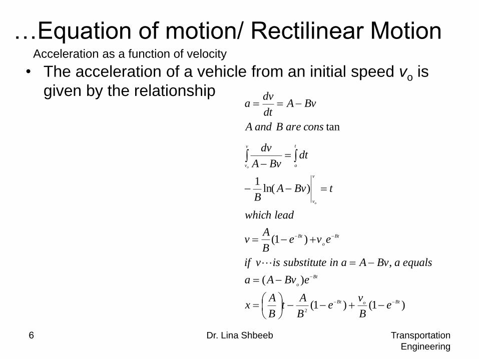
…Equation of motion/ Rectilinear Motion
• The acceleration of a vehicle from an initial speed vo is
given by the relationship
Acceleration as a function of velocity
)1()1(
)(
,
)1(
)ln(1
tan
2
BtoBt
Bt
o
Bt
o
Bt
v
v
t
o
v
v
eB
ve
B
At
B
Ax
eBvAa
equalsaBvAainsubstituteisvif
eveB
Av
leadwhich
tBvAB
dtBvA
dv
consareBandA
BvAdt
dva
o
o

Dr. Lina Shbeeb
Travel Speed
12
12
tt
xxv
Time
Distance
t2
t1
x1
x2

Dr. Lina Shbeeb
Spot Speed
dt
dxv
Time
Distance
t1
x1
V

Dr. Lina Shbeeb
Spot Speed Measurements
t1 t2 t3 Time
x3
x2
x1
Dis
tance
45.0
40.0
30.0
Distance
x
(ft)
4.0
3.0
2.0
Time
t
(s)
(40-30)/(3-2)
=10.0
---
Speed 1
v
(ft/s)
---
(45-30)/(4-2)
= 7.5
---
Speed 2
v
(ft/s)
(45-40)/(3-2)
=5.0

Dr. Lina Shbeeb
Spot Speed Measurements
Time
(s)
Distance
(ft)
Speed
(ft)
0.0 0.0 -
0.1 2.13 21.5
0.2 4.30 21.9
0.3 6.51 22.4
0.4 8.78 22.4
0.5 10.99 21.3
0.6 13.04 -
Dr. Lina Shbeeb
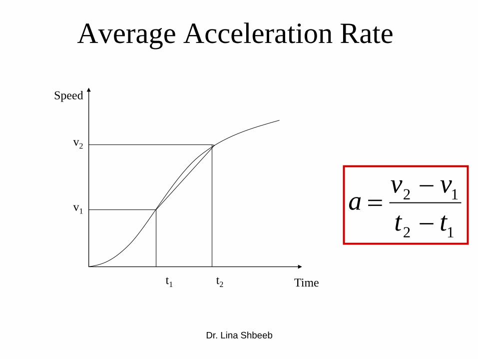
Average Acceleration Rate
12
12
tt
vva
Time
Speed
t2
t1
v1
v2

Dr. Lina Shbeeb
Spot Acceleration Rate
dt
dva
Time
speed
t1
v1
a

Dr. Lina Shbeeb
Measuring Acceleration
Rates
Time
(s)
Distance
(ft)
Speed
(ft/s)
Acceleration
(ft/s2)
0.0 0.0 - -
0.1 2.13 21.5 -
0.2 4.30 21.9 4.5
0.3 6.51 22.4 2.5
0.4 8.78 22.4 -5.5
0.5 10.99 21.3 -
0.6 13.04 - -

Dr. Lina Shbeeb
Constant Acceleration Motion
constadt
dv
tv
vadtdv
00
0vatv
avdx
dv
xv
vadxvdv
00
a
vvx
2
20
2
dtvatvdtdx )( 0
x t
dtvatdx0 0 0 )(
tvatx 0
2
2
1
Remark: The equation used for design is , where the
deceleration rate has a positive value.
a
vvx
2
220

Dr. Lina Shbeeb
Exercise
•From the following data,
calculate the acceleration
rate at the distance of 2
feet from the reference
point.
Distance
(ft) Speed
(ft/s)
0 19.4
1 19.6
2 20.0
3 20.8
4 21.3
a=5.91ft/s2???

Transportation
Engineering
Dr. Lina Shbeeb 16
Constant Acceleration Motion
constadt
dv
tv
vadtdv
00
0vatv
avdx
dv
xv
vadxvdv
00
a
vvx
2
20
2
dtvatvdtdx )( 0
x t
dtvatdx0 0 0 )(
tvatx 0
2
2
1
Remark: The equation used for design is , where the
deceleration rate has a positive value.
a
vvx
2
220
Transportation
Engineering
Dr. Lina Shbeeb 17
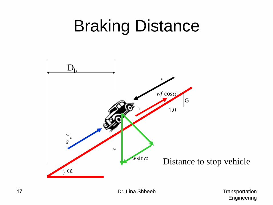
Braking Distance
ag
w
w
sinw
u
coswf
Db
G
1.0
Distance to stop vehicle

Transportation
Engineering
Dr. Lina Shbeeb 18
Braking on Grades
sincos WWfag
W
a
vvx
2
220
x
Db
cos2
cos22
0
a
vvxDb
bDvva
2
cos)( 22
0
cos
sincos2
cos)(
1 220
f
Dvv
g b
cos
sin
2
1)(
1 220
f
Dvv
g b
G
tan
cos
sin)(2
220
Gfg
vvDb
Transportation
Engineering
Dr. Lina Shbeeb 19
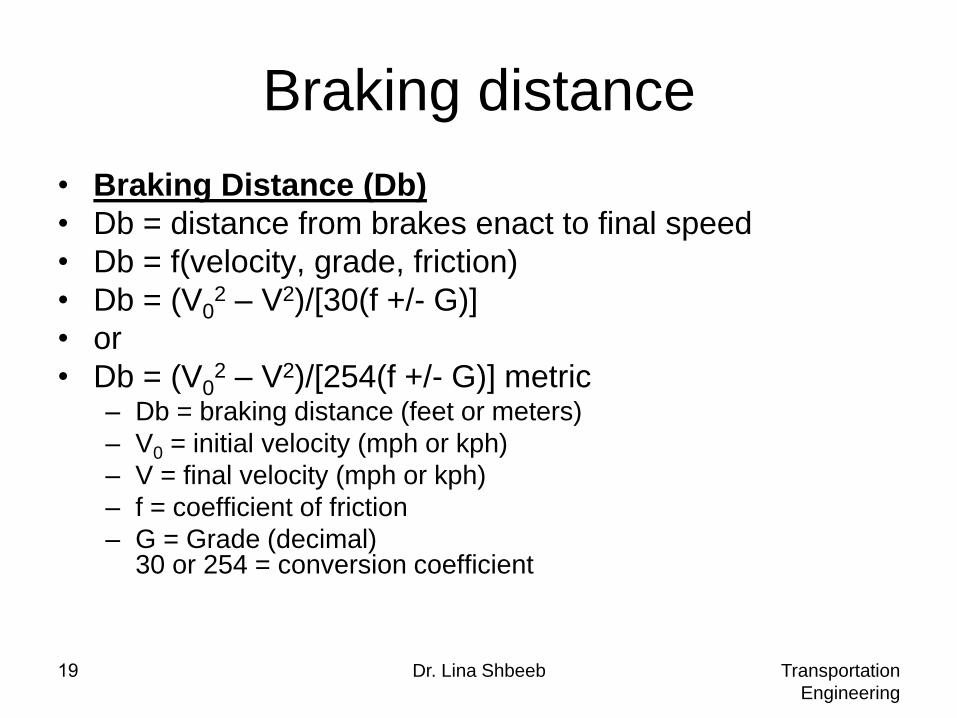
Braking distance
• Braking Distance (Db)
• Db = distance from brakes enact to final speed
• Db = f(velocity, grade, friction)
• Db = (V02 – V2)/[30(f +/- G)]
• or
• Db = (V02 – V2)/[254(f +/- G)] metric
– Db = braking distance (feet or meters)
– V0 = initial velocity (mph or kph)
– V = final velocity (mph or kph)
– f = coefficient of friction
– G = Grade (decimal) 30 or 254 = conversion coefficient
Transportation
Engineering
Dr. Lina Shbeeb 20
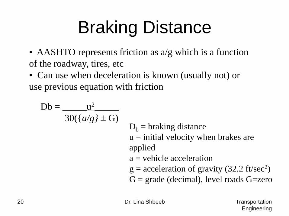
Braking Distance
Db = braking distance
u = initial velocity when brakes are
applied
a = vehicle acceleration
g = acceleration of gravity (32.2 ft/sec2)
G = grade (decimal), level roads G=zero
• AASHTO represents friction as a/g which is a function
of the roadway, tires, etc
• Can use when deceleration is known (usually not) or
use previous equation with friction
Db = _____u2_____
30({a/g} ± G)
Transportation
Engineering
Dr. Lina Shbeeb 21
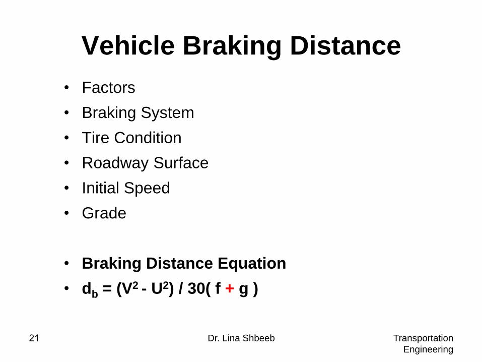
Vehicle Braking Distance
• Factors
• Braking System
• Tire Condition
• Roadway Surface
• Initial Speed
• Grade
• Braking Distance Equation
• db = (V2 - U2) / 30( f + g )

Transportation
Engineering
Dr. Lina Shbeeb 22
Coefficient of friction
Pavement condition Maximum Slide
Good, dry 1.00 0.80
Good, wet 0.90 0.60
Poor, dry 0.80 0.55
Poor, wet 0.60 0.30
Packed snow and
Ice
0.25 0.10
Transportation
Engineering
Dr. Lina Shbeeb 23
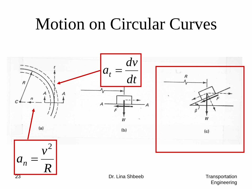
Motion on Circular Curves
dt
dvat
R
van
2

Transportation
Engineering
Dr. Lina Shbeeb 24
coscossin ns amWfW
coscos)(cossin
2
WR
v
g
WWfW s
e
tan
cos
sin
gR
vfe s
2
Motion on
Circular
Curves

Transportation
Engineering
Dr. Lina Shbeeb 25
Minimum Radius of a Circular Curve
• where u = vehicle velocity (mph)
• e = tan (rate of superelevation)
• fs = coefficient of side friction (depends on design speed)
• Example
– design speed = 65 mph
– rate of superelevation = 0.05
– coefficient of side friction = 0.11
• Solution
– minimum radius
– R = (65)2/[15(0.05+0.11)] = 1760 ft
)(15
2
sfe
uR

Transportation
Engineering
Dr. Lina Shbeeb 26
Relative Motion • It is common to examine the motion of one
object in relation to another, for example the
motion of vehicles on a highway may be studies
from the point of view of the driver of a moving
vehicle.
• The simplest case of relative motion involves the
motion of one object B relative to a coordinate
system (x, y, z) that is translating but not rotating
with respect to a fixed coordinate system (X, Y,
Z)

Transportation
Engineering
Dr. Lina Shbeeb 27
Relative Motion • The relationship between the position vectors of the two objects in relation to the fixed
system, RA and RB and the position vector rB/A with respect to the moving object A is
Y
Z
y
X
x
z
RA
RB
RA/B
ABAB
ABAB
ABAB
aaa
and
vvv
givestimetorespectwithatingDifferenti
rrr
/
/
/


