MEDICAL IMAGE COMPUTING (CAP 5937) LECTURE 4: Pre-Processing Medical Images (II) Dr. Ulas Bagci HEC 221, Center for Research in Computer Vision (CRCV), University of Central Florida (UCF), Orlando, FL 32814. [email protected]or [email protected]1 SPRING 2017
Transcript
MEDICAL IMAGE COMPUTING (CAP 5937)
LECTURE 4: Pre-Processing Medical Images (II)
Dr. Ulas BagciHEC 221, Center for Research in Computer Vision (CRCV), University of Central Florida (UCF), Orlando, FL [email protected] or [email protected]
1SPRING 2017
Outline• Diffusion based Smoothing in Medical Scans• Intensity inhomogeneity Correction in MRI
• Perona and Malik propose a nonlinear diffusion method for avoiding the blurring and localization problems of linear diffusion filtering [PAMI 1990].– Smooth the images without removing significant parts of the edges
5
Perona-Malik (Anisotropic Diffusion) Filtering
• Perona and Malik propose a nonlinear diffusion method for avoiding the blurring and localization problems of linear diffusion filtering [PAMI 1990].– Smooth the images without removing significant parts of the edges– The smoothing process is considered as diffusion
6
Perona-Malik (Anisotropic Diffusion) Filtering
• Perona and Malik propose a nonlinear diffusion method for avoiding the blurring and localization problems of linear diffusion filtering [PAMI 1990].– Smooth the images without removing significant parts of the edges– The smoothing process is considered as diffusion– APPROACH: Increase the diffusivity of filter for large (homogeneous)
regions, and decrease it nearby edges!
7
Perona-Malik (Anisotropic Diffusion) Filtering
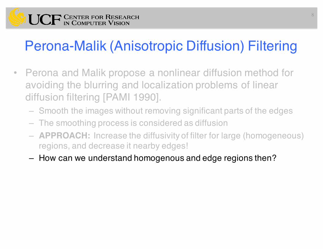
• Perona and Malik propose a nonlinear diffusion method for avoiding the blurring and localization problems of linear diffusion filtering [PAMI 1990].– Smooth the images without removing significant parts of the edges– The smoothing process is considered as diffusion– APPROACH: Increase the diffusivity of filter for large (homogeneous)
regions, and decrease it nearby edges!– How can we understand homogenous and edge regions then?
8
Perona-Malik (Anisotropic Diffusion) Filtering
• Perona and Malik propose a nonlinear diffusion method for avoiding the blurring and localization problems of linear diffusion filtering [PAMI 1990].– Smooth the images without removing significant parts of the edges– The smoothing process is considered as diffusion– APPROACH: Increase the diffusivity of filter for large (homogeneous)
regions, and decrease it nearby edges!– How can we understand homogenous and edge regions then?– Edge likelihood (i.e, gradient for instance) can be measured by
9
Perona-Malik (Anisotropic Diffusion) Filtering
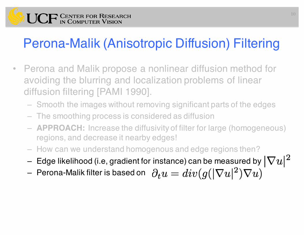
• Perona and Malik propose a nonlinear diffusion method for avoiding the blurring and localization problems of linear diffusion filtering [PAMI 1990].– Smooth the images without removing significant parts of the edges– The smoothing process is considered as diffusion– APPROACH: Increase the diffusivity of filter for large (homogeneous)
regions, and decrease it nearby edges!– How can we understand homogenous and edge regions then?– Edge likelihood (i.e, gradient for instance) can be measured by– Perona-Malik filter is based on
10
Perona-Malik (Anisotropic Diffusion) Filtering
• Perona and Malik propose a nonlinear diffusion method for avoiding the blurring and localization problems of linear diffusion filtering [PAMI 1990].– Smooth the images without removing significant parts of the edges– The smoothing process is considered as diffusion– APPROACH: Increase the diffusivity of filter for large (homogeneous)
regions, and decrease it nearby edges!– How can we understand homogenous and edge regions then?– Edge likelihood (i.e, gradient for instance) can be measured by– Perona-Malik filter is based on
where it uses diffusivities such as
11
Perona-Malik (Anisotropic Diffusion) Filtering
• Perona and Malik propose a nonlinear diffusion method for avoiding the blurring and localization problems of linear diffusion filtering [PAMI 1990].– Smooth the images without removing significant parts of the edges– The smoothing process is considered as diffusion– APPROACH: Increase the diffusivity of filter for large (homogeneous)
regions, and decrease it nearby edges!– How can we understand homogenous and edge regions then?– Edge likelihood (i.e, gradient for instance) can be measured by– Perona-Malik filter is based on
where it uses diffusivities such as
– approximation
12
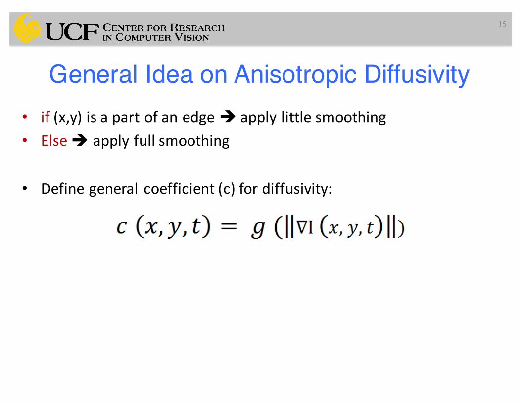
General Idea on Anisotropic Diffusivity• if (x,y)isapartofanedgeè applylittlesmoothing• Elseè applyfullsmoothing
13
General Idea on Anisotropic Diffusivity• if (x,y)isapartofanedgeè applylittlesmoothing• Elseè applyfullsmoothing• Assume,Eisedgelikelihood(tellingyouifyouareinhomogeneous
oredgeregions)• CONTROLLINGTHEBLURRING(SMOOTHING)
or
14
General Idea on Anisotropic Diffusivity• if (x,y)isapartofanedgeè applylittlesmoothing• Elseè applyfullsmoothing
• Definegeneralcoefficient(c)fordiffusivity:
15
General Idea on Anisotropic Diffusivity• if (x,y)isapartofanedgeè applylittlesmoothing• Elseè applyfullsmoothing
• Definegeneralcoefficient(c)fordiffusivity:
16
d=1,… direction
General Idea on Anisotropic Diffusivity• if (x,y)isapartofanedgeè applylittlesmoothing• Elseè applyfullsmoothing
• Definegeneralcoefficient(c)fordiffusivity:
17
Isotropic: Anisotropic:
Toy Example18
Original Linearisotropicdiffusion(simpleGaussian)
Toy Example19
Original Non-linearanisotropicdiffusion
20
21
Non-linear Diffusion
Background: BrainWeb
22
WM
GM
CSF MR Brain simulator
Magnetic Field Inhomogeneity23
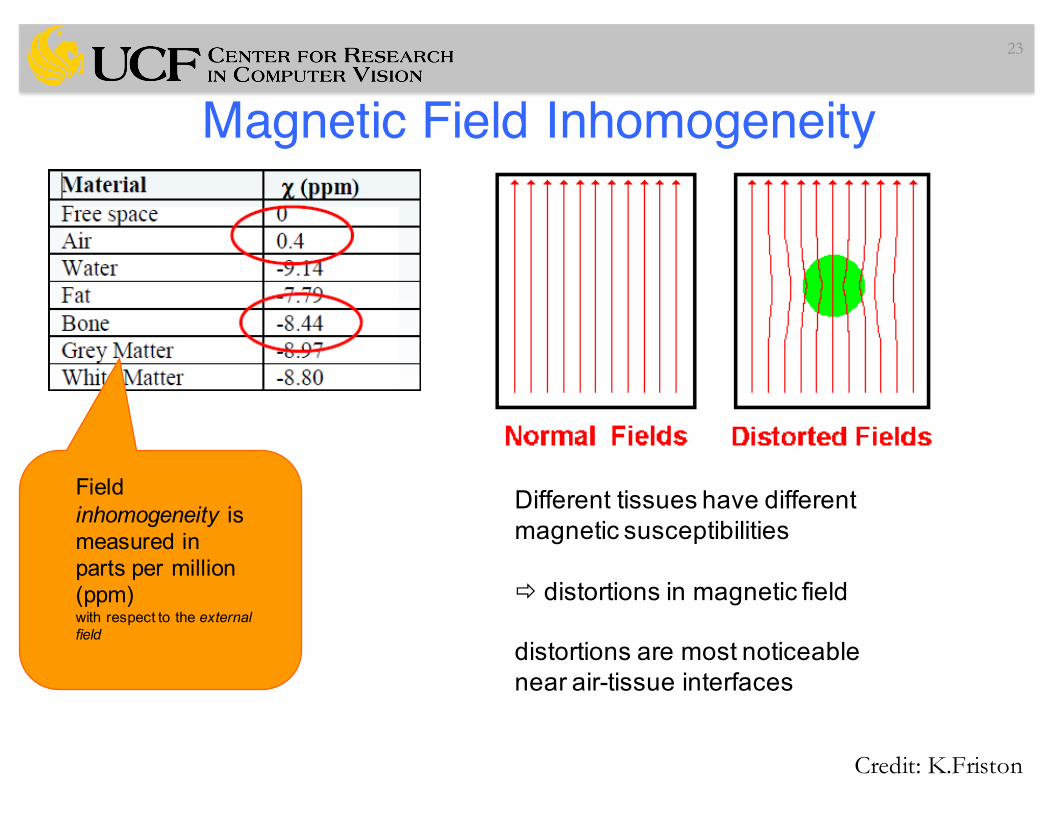
Field inhomogeneity is measured in parts per million (ppm) with respect to the external field
Different tissues have different magnetic susceptibilities
ð distortions in magnetic field
distortions are most noticeable near air-tissue interfaces
Credit: K.Friston
MR Intensity Inhomogeneity• Often hardly
noticeable, but registration, segmentation, and thus quantificationprocesses are significantly affected from inhomogeneity field
24
(credit: R.Gupta)
MR Intensity Inhomogeneity
25
(credit: R.Gupta)
Large susceptibility variation in the human brain leads to greater field inhomogeneity and therefore image distortion.
Intensity Inhomogeneity Correction• Problem:
– Imperfections in the RF field cause background variations in MRimages.
– Poses challenges in image segmentation and analysis.
• Goal: To develop a general method for correcting the variations that fulfills:– (R1) no need for user help per scene– (R2) no need for accurate prior segmentation
– (R3) no need for prior knowledge of tissue intensity distribution
26
Intensity Inhomogeneity Correction Methods
27
Original Image Inhomogeneity Field Corrected Image
Bias Correction ApproachesNumerous methods have been published in the last two decades
I. Prospective Approachesi. Phantomii. Multicoiliii. Special sequence
II. Retrospective Approachesi. Filteringii. Surface Fitting (intensity or gradient)iii. Segmentation (ML, MAP, FCM, nonparametric,…)iv. Histogram
a. High frequency maximizationb. Information amximizationc. Histogram matching
28
Prospective Approaches-Phantom• Treat intensity corruption as a systematic error of the MRI
acquisition process that can either be minimized by acquiring additional images of a uniform phantom, by acquiring additional images with different coils, or by devising special imaging sequences.
29
Prospective Approaches-Phantom• Treat intensity corruption as a systematic error of the MRI
acquisition process that can either be minimized by acquiring additional images of a uniform phantom, by acquiring additional images with different coils, or by devising special imaging sequences.
• Oil or water is usually used for phantoms and median filtering is applied for image smoothing.
30
Prospective Approaches-Phantom• Treat intensity corruption as a systematic error of the MRI
acquisition process that can either be minimized by acquiring additional images of a uniform phantom, by acquiring additional images with different coils, or by devising special imaging sequences.
• Oil or water is usually used for phantoms and median filtering is applied for image smoothing.
• Warning: The phantom based approach cannot correct for patient-induced inhomogeneity, which is a major drawback of this approach. The remaining intensity inhomogeneity can be as high as 30%
31
Prospective Approaches-MultiCoil and Special Sequences
• Volume and Surface coils– Volume coil: induce less inhomogeneity, poor SNR– Surface coil: induce severe inhomogeneity, good SNR– Method: dividing the filtered surface coil image with the body coil
image and smoothing the resulting image– Disadvantage: prolonged acquisition time
32
Prospective Approaches-MultiCoil and Special Sequences
• Volume and Surface coils– Volume coil: induce less inhomogeneity, poor SNR– Surface coil: induce severe inhomogeneity, good SNR– Method: dividing the filtered surface coil image with the body coil
image and smoothing the resulting image– Disadvantage: prolonged acquisition time
• Sequence design (pulse design)– Method: the spatial distribution of the flip angle can be estimated and
used to calculate the intensity inhomogeneity. – Disadvantage: Hardware design
33
Retrospective Approaches– Only a few assumptions are needed, therefore these approaches are
general.
34
Retrospective Approaches– Only a few assumptions are needed, therefore these approaches are
general.– Unlike prospective approaches, these approaches can also correct
patient dependent inhomogeneities apart from scanner induced inhomogeneities.
35
Retrospective Approaches– Only a few assumptions are needed, therefore these approaches are
general.– Unlike prospective approaches, these approaches can also correct
patient dependent inhomogeneities apart from scanner induced inhomogeneities.
– FILTERING:• Filtering methods assume that intensity inhomogeneity is a low-frequency
artifact that can be separated from the high-frequency signal of the imaged anatomical structures by low-pass filtering
36
Retrospective Approaches– Only a few assumptions are needed, therefore these approaches are
general.– Unlike prospective approaches, these approaches can also correct
patient dependent inhomogeneities apart from scanner induced inhomogeneities.
– FILTERING:• Filtering methods assume that intensity inhomogeneity is a low-frequency
artifact that can be separated from the high-frequency signal of the imaged anatomical structures by low-pass filtering
• log v(x) is input image, CN is normalization constant, u(x) corrected image.• However, this is true only when imaged anatomical structures are
relatively small !!!
37
Retrospective Approaches– Only a few assumptions are needed, therefore these approaches are
general.– Unlike prospective approaches, these approaches can also correct
patient dependent inhomogeneities apart from scanner induced inhomogeneities.
– FILTERING:• Homomorphic unsharp masking• probably the simplest and one of the most commonly used methods• b(x) (bias field) is obtained by low-pass filtering of the input image v(x),
divided by the constant CN to preserve mean or median intensity
38
Prospective Approaches-Filtering/Surface Fitting
39
A representative example of a slice from a rat brain. a: Original image. b: after inhomogeneity correction with the phantom based correction algorithm. Credit: Hui et al, JMRI 2010.
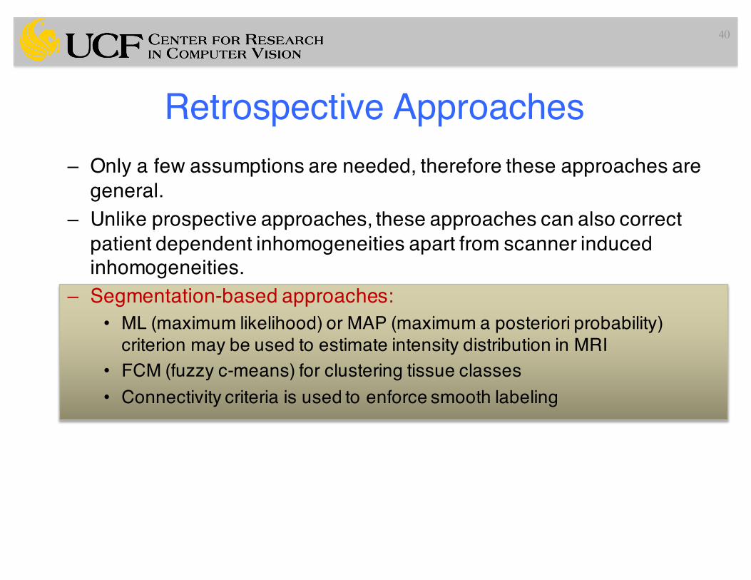
Retrospective Approaches– Only a few assumptions are needed, therefore these approaches are
general.– Unlike prospective approaches, these approaches can also correct
patient dependent inhomogeneities apart from scanner induced inhomogeneities.
– Segmentation-based approaches:• ML (maximum likelihood) or MAP (maximum a posteriori probability)
criterion may be used to estimate intensity distribution in MRI• FCM (fuzzy c-means) for clustering tissue classes• Connectivity criteria is used to enforce smooth labeling
40
Retrospective Approaches– Only a few assumptions are needed, therefore these approaches are
general.– Unlike prospective approaches, these approaches can also correct
patient dependent inhomogeneities apart from scanner induced inhomogeneities.
– Histogram-based approaches:• directly on image intensity histograms• the inhomogeneity field is slowly varying -> it is natural to assume smooth
histogram then!• N3 method is widely used, the method is iterative and seeks the smooth
multiplicative field that maximizes the high frequency content of the distribution of tissue intensity.
• Consider the following model of image formation in MR:
where at location x, v is measured signal, u is true signal, n is noise. f (bias field) is unknown.• For a noise-free case, to estimate f requires some math.
• Consider the following model of image formation in MR:
where at location x, v is measured signal, u is true signal, n is noise. f (bias field) is unknown.• For a noise-free case, to estimate f requires some math.
• Consider the following model of image formation in MR:
where at location x, v is measured signal, u is true signal, n is noise. f (bias field) is unknown.• For a noise-free case, to estimate f requires some math.
• Consider the following model of image formation in MR:
where at location x, v is measured signal, u is true signal, n is noise. f (bias field) is unknown.• For a noise-free case, to estimate f requires some math.
tricks such as
• Let U,V, and F be the probability densities of• (approx.) if u and f are uncorrelated random variables, then
47
if u and f are uncorrelated random variables, the distribution of their sum is found by
Local Histogram Based and Standardization Based Correction Methods
• Dividing the image into small subvolumes (via fixed thresholding for instance) in which intensity inhomogeneity was supposed to be relatively constant.
58
Local Histogram Based and Standardization Based Correction Methods
• Dividing the image into small subvolumes (via fixed thresholding for instance) in which intensity inhomogeneity was supposed to be relatively constant.
• Standard intensity scale is assumed (NEXT LECTURE)– Similar intensity values are assigned to similar tissues across different
images
59
Local Histogram Based and Standardization Based Correction Methods
• Dividing the image into small subvolumes (via fixed thresholding for instance) in which intensity inhomogeneity was supposed to be relatively constant.
• Standard intensity scale is assumed (NEXT LECTURE)– Similar intensity values are assigned to similar tissues across different
images• Local intensity inhomogeneity was estimated by least square
fitting of the intensity histogram model to the actual histogram of a subvolume
60
Local Histogram Based and Standardization Based Correction Methods
• Dividing the image into small subvolumes (via fixed thresholding for instance) in which intensity inhomogeneity was supposed to be relatively constant.
• Standard intensity scale is assumed (NEXT LECTURE)– Similar intensity values are assigned to similar tissues across different
images• Local intensity inhomogeneity was estimated by least square
fitting of the intensity histogram model to the actual histogram of a subvolume
• The applied histogram model was a finite Gaussian mixture with seven parameters, initialized from the global histogram of the image. (B-splines are used to fit parameters)
61
Better (Simpler) Method – Standardization Based Correction (SBC)
Step 0: Set Sc = S, the given scene.
Step 1: Standardize Sc to the standard intensity gray scalefor the particular imaging protocol and body regionunder consideration and output scene Ss;
Step 2: determine m tissue regions SB1, SB2, ..., SBm by usingfixed threshold intervals on Ss;
Step 3: if SBi determined in the previous iteration are notmuch (<0.1%) different from the current SBi, stop;
Step 4: else, estimate background variation in Ss as a sceneSbe, compute corrected scene Sc, and go to Step 1;
62
SBC-Intuition
63
Oi Oj x
( )j xβ
( )i xβ
The existence of discontinuity between inhomogeneity maps (continuous lines) estimated independently from different tissue regions Oi and Oj.
We need a single combined inhomogeneity map for correcting the background intensity variation in the whole image.
SBC-Intuition
64
1. Find a weight factor λ to minimize
2. Combine the two inhomogeneity maps β1 and β2 to obtain a new discrete inhomogeneity map βd(c): C → [0, ∞) such that, for any c∈C,
3. Determine a 2nd degree polynomial β that constitutes a LSE fit to βd .
The above steps merge O1 and O2 and are then repeated until we have only one region and a single unified inhomogeneity map.
( ) ( ) 21 2 .
c Cc cβ λβ
∈
⎡ ⎤−⎣ ⎦∑
( ) ( )( ) ( ) ( ) ( )
( ) ( ) ( )2 11 2
1 2 1 2
, ,
, , , ,d
c O c Oc c c
c O c O c O c Oδ δ
β β λβδ δ δ δ
= ++ +
65
Original Corrected
Standardization Based Correction (SBC) Method
66
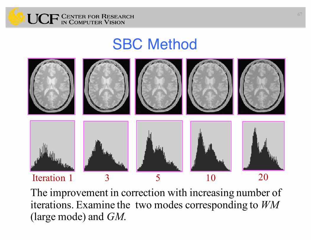
Iteration 1 3 5 10 20
GM
WM
SBC Method
67
Iteration 1 3 5 10 20The improvement in correction with increasing number of iterations. Examine the two modes corresponding to WM(large mode) and GM.
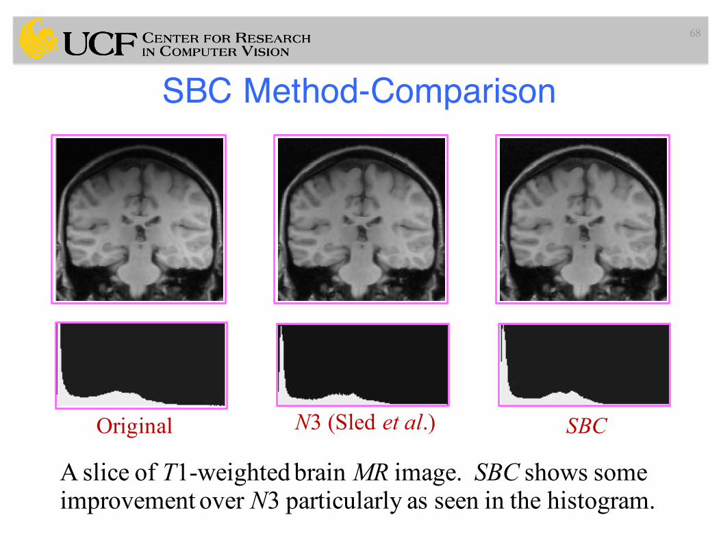
SBC Method-Comparison
68
Original N3 (Sled et al.) SBC
A slice of T1-weighted brain MR image. SBC shows some improvement over N3 particularly as seen in the histogram.
SBC Method-Comparison
69
Original N3 (Sled et al.) SBC
A slice of an abdominal MR image. SBC shows some improvement over N3 particularly as seen in the histogram.
SBC Method-Comparison
70
Original N3 (Sled et al.) SBC
Brainweb T2-weighted MR image. SBC shows some improvement over N3 particularly as seen in the histogram.
Coefficient of Variation as a quantitative evaluation metric
• CV (coefficient of variation)?
71
Coefficient of Variation as a quantitative evaluation metric
• CV (coefficient of variation):
72
Coefficient of Variation as a quantitative evaluation metric
• CV (coefficient of variation):
• For a given tissue class C, CV shows how much intensity inhomogeneity is introduced (existed)
73
Coefficient of Variation as a quantitative evaluation metric
• CV (coefficient of variation):
• For a given tissue class C, CV shows how much intensity inhomogeneity is introduced (existed)
• There are some drawbacks in using CV!
74
Coefficient of Variation as a quantitative evaluation metric
• CV (coefficient of variation):
• For a given tissue class C, CV shows how much intensity inhomogeneity is introduced (existed)
• There are some drawbacks in using CV!– Single tissue class is used C, (alternatively Coef. Of Joint Variation can
be used)
75
Coefficient of Variation as a quantitative evaluation metric
• CV (coefficient of variation):
• For a given tissue class C, CV shows how much intensity inhomogeneity is introduced (existed)
• There are some drawbacks in using CV!– Single tissue class is used C, (alternatively Coef. Of Joint Variation can
be used)– Sensitive to brightness of the image (change the mean, not the std)
76
Coefficient of Variation as a quantitative evaluation metric
• CV (coefficient of variation):
• For a given tissue class C, CV shows how much intensity inhomogeneity is introduced (existed)
• There are some drawbacks in using CV!– Single tissue class is used C, (alternatively Coef. Of Joint Variation can
be used)– Sensitive to brightness of the image (change the mean, not the std)– …
77
SBC Method Quantitative Comparison
78
%cv (GM) %cv (WM) Set Modality Inhomo. Original N3 SBC Original N3 SBC
Normal
T1 20% 40%
11.0 13.5
9.9 10.0
9.9 9.9
6.7 9.2
5.1 5.2
5.1 5.2
T2 20% 40%
18.4 20.3
18.0 20.0
17.9 17.9
12.0 13.3
11.8 13.0
11.7 11.8
PD 20% 40%
6.3 9.7
4.6 4.6
4.5 4.5
5.5 7.5
4.7 4.6
4.7 4.6
Ms Lesions
T1 20% 40%
11.2 13.7
10.1 10.2
10.1 10.1
6.9 9.3
5.3 5.3
5.3 5.4
T2 20% 40%
10.9 13.7
10.0 10.1
9.8 9.8
8.7 10.6
8.3 8.2
8.1 8.2
PD 20% 40%
5.8 9.4
3.9 4.9
3.8 3.9
5.3 7.4
4.4 4.3
4.3 4.3
% cv of tissue intensities in segmented GM and WMregions for twelve simulated MRI scenes from Brainwebbefore and after correction by N3 SBC.
SBC Method Quantitative Comparison
79
Modality % cv (GM) % cv (WM)
Original N3 SBC Original N3 SBC T2 16.7(1.61) 14.9(1.18) 14.7(1.23) 12.9(1.12) 11.5(1.07) 11.2(0.98) PD 7.1(0.32 5.9(0.20) 5.6(0.19) 7.8(0.72) 6.6(0.62) 6.2(0.51)
The mean and standard deviation of % cv of tissue intensities in segmented GM and WM regions for ten clinical T2- and PD-weighted MRI scenes of MS patients before and after correction by the N3 and SBC methods.
SBC > N3; p < 0.001.
References and Slide Credits• Jayaram K. Udupa, MIPG of University of Pennsylvania, PA.• P. Suetens, Fundamentals of Medical Imaging, Cambridge
Univ. Press.• N. Bryan, Intro. to the science of medical imaging, Cambridge
Univ. Press.• N. Agam (toy examples)
• Next Lecture (Preprocessing of Medical Images III)– Intensity Standardization in MR Images– PET/SPECT Image Denoising (multiplicative noise)