203
NEURAL NETWORKS НЕЙРОННІ МЕРЕЖІ Лекція 2
| Date post: | 09-Aug-2015 |
| Category: |
Education |
| Upload: | halyna-melnyk |
| View: | 46 times |
| Download: | 1 times |

NEURAL NETWORKSНЕЙРОННІ МЕРЕЖІЛекція 2

Як нейрони і “нейрони” працюють?
Штучна нейронна мережа

… приблизно так він виглядає
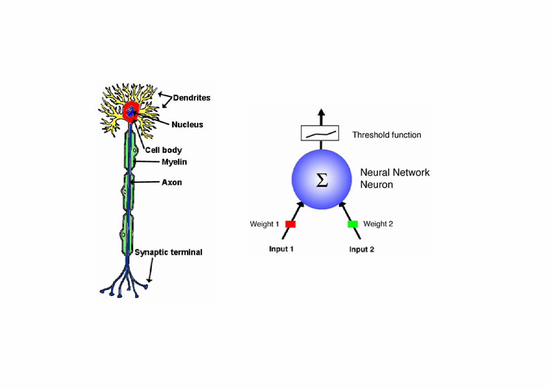
Нейрон людини
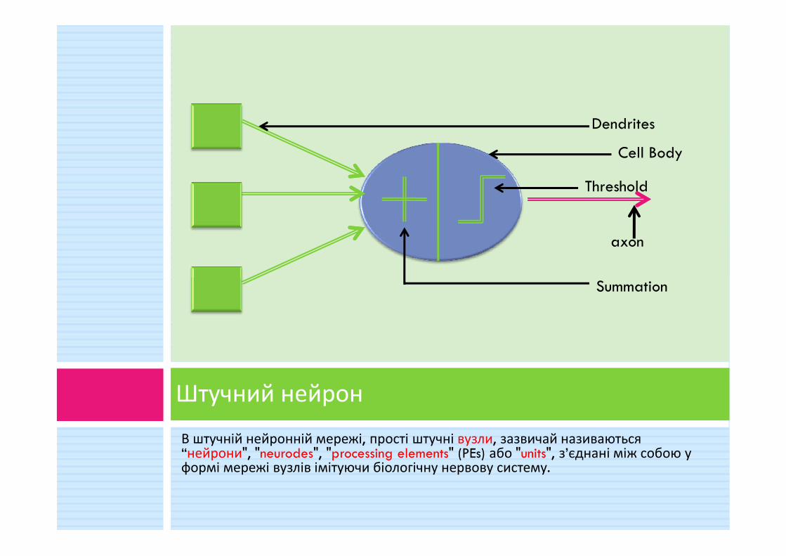
Dendrites
Cell Body
Threshold
axon
Summation
В штучній нейронній мережі, прості штучні вузли, зазвичай називаються “нейрони", "neurodes", "processing elements" (PEs) або "units", з’єднані між собою у формі мережі вузлів імітуючи біологічну нервову систему.
Штучний нейрон
Summation
Покращений нейрон
W1W1
W2W2
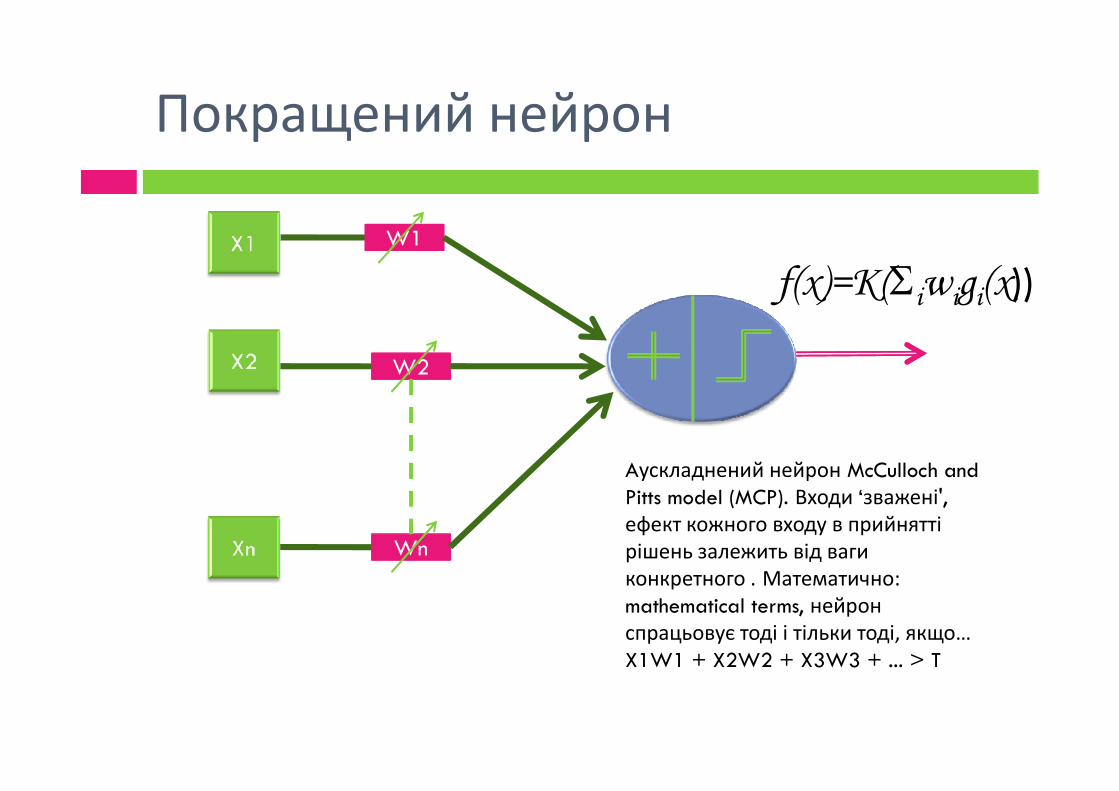
f(x)=K(iwigi(x))
WnWn
Aускладнений нейрон McCulloch and Pitts model (MCP). Входи ‘зважені', ефект кожного входу в прийнятті рішень залежить від ваги конкретного . Математично: mathematical terms, нейрон спрацьовує тоді і тільки тоді, якщо…X1W1 + X2W2 + X3W3 + ... > T

Модель НМ
Найбільш поширений тип штучної нейронної мережі складається з трьох груп, або шарів, блоків:
шар "input" units, пов'язаних з діяльністю вхідних блоків являє собою необроблену являє собою необроблену інформацію, яка подається в мережу.
шар "hidden" units, діяльність кожного прихованого блоку визначається діяльністю вхідних вузлів і ваг на зв'язку між входом і прихованими елементами.
шар "output" units. Поведінка вихідних units залежить від діяльності прихованих units.
Будова НМ
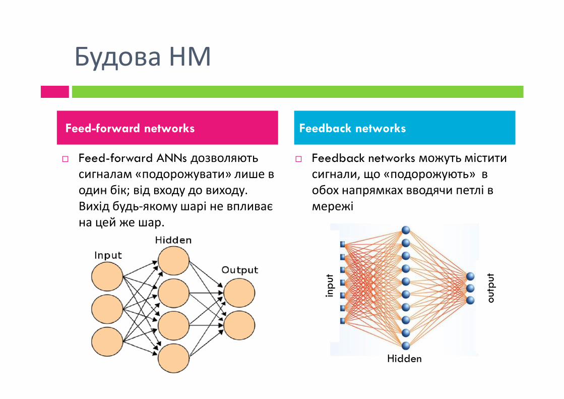
Feed-forward ANNs дозволяють сигналам «подорожувати» лише в один бік; від входу до виходу. Вихід будь-якому шарі не впливає
Feedback networks можуть містити сигнали, що «подорожують» в обох напрямках вводячи петлі в мережі
Feed-forward networks Feedback networks
Вихід будь-якому шарі не впливає на цей же шар.
мережі
inp
ut
Hidden
outp
ut

Правило спрацьовування (Firing rule )
The firing rule пояснює високу гнучкість НМ.
A firing rule визначає при обчисленні чи буде спрацьовувати нейрон для будь-якого вхідного набору. Це відноситься до всіх вхідних шаблонів, а не тільки тих, на яких навчався вузол.тільки тих, на яких навчався вузол.

Візьміть колекцію шаблонів для навчання вузла, входи в які
примушують спрацьовувати -1 забороняють спрацьовування - 0 Які із зразків не в колекції?? Які із зразків не в колекції??
вузол спрацьовує, коли в порівнянні він має в загальному більше вхідних елементів з набором «найближчим» до 1- «навченої» множини ніж вхідних елементів з набором «найближчим» до 0- «навченої» множини.
якщо є петля, то набір залишається у невизначеному стані.

приклад
3-вхідний нейрон навчений ЯК:
Вихід 1 коли вхід (X1,X2 і X3) -111, 101 Вихід 1 коли вхід (X1,X2 і X3) -111, 101
Вихід 0 коли вхід 000 або 001

X1 0 0 0 0 1 1 1 1
X2 0 0 1 1 0 0 1 1
X3 0 1 0 1 0 1 0 1
Out 0 0 0/1 0/1 0/1 1 0/1 1
До узагальнення
111, 101=1 000 or 001=0
X1 0 0 0 0 1 1 1 1
X2 0 0 1 1 0 0 1 1
X3 0 1 0 1 0 1 0 1
Out 0 0 0 0/1 0/1 1 1 1
Out 0 0 0/1 0/1 0/1 1 0/1 1
Після узагальнення

Розпізнавання наборів
TAN1
F1
X11
X12
X13
X21
X22F2
F3
X22
X23
X31
X32
X33
TAN2
TAN3
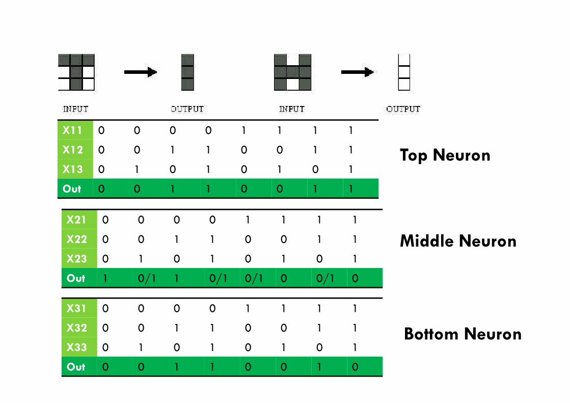
X11 0 0 0 0 1 1 1 1
X12 0 0 1 1 0 0 1 1
X13 0 1 0 1 0 1 0 1
Out 0 0 1 1 0 0 1 1
Top Neuron
X21 0 0 0 0 1 1 1 1
X22 0 0 1 1 0 0 1 1
X23 0 1 0 1 0 1 0 1
Out 1 0/1 1 0/1 0/1 0 0/1 0
X31 0 0 0 0 1 1 1 1
X32 0 0 1 1 0 0 1 1
X33 0 1 0 1 0 1 0 1
Out 0 0 1 1 0 0 1 0
Middle Neuron
Bottom Neuron


• Багато нейронів типу PEs units
– Input & output units отримують та передають імпульси (сигнали) відповідно з/в оточення
– Внутрішні units називаються hidden units оскільк вони не контактують з оточенням
– з’єднані weighted links (синапсами)
• A parallel computation system оскільки
– Іпульси передаються незалежно по зваженим каналам & units та можуть оновлювати свій стан паралельно
– Однак, більшість NNs можуть бути симуоьовані на серійних компютерах
Штучна нейронна мережа
– Однак, більшість NNs можуть бути симуоьовані на серійних компютерах
• directed graph, з маркованими зваженими типово використовується для опису з’єднань між units

activationlevel
A NODE
inig
ai
inputfunction
activation functionoutput
input linksoutputlinks
aj Wj,i
ai = g(ini)
Кожен блок обробки має просту програму, яка:• обчислює зважену суму вхідних даних, отриманих від units• видає єдине значення, яке в цілому є нелінійною функцією зваженої суми входів --- це вихід стає вхідним сигналом для тих units до яких він передає імпульс

g = Activation functions for units
Step function(Linear Threshold Unit)
Sign function Sigmoid function
step(x) = 1, if x >= threshold0, if x < threshold
sign(x) = +1, if x >= 0-1, if x < 0
sigmoid(x) = 1/(1+e-x)
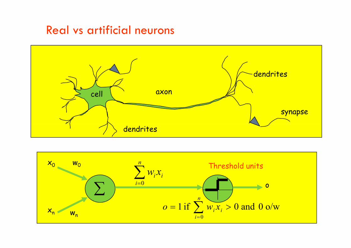
Real vs artificial neurons
axon
dendrites
dendrites
synapse
cell
dendrites
x0
xn
w0
wn
o
i
n
ii xw
0
o/w 0 and 0 if 10
i
n
ii xwo
Threshold units

Artificial neurons
Neurons work by processing information. They receive and provide information in form of spikes.
w1
x1
x2
The McCullogh-Pitts model
Inputs
Outputw2
w1
w3
wn
wn-1
..
.
2
x3
…
xn-1
xn
y)(;
1
zHyxwzn
iii
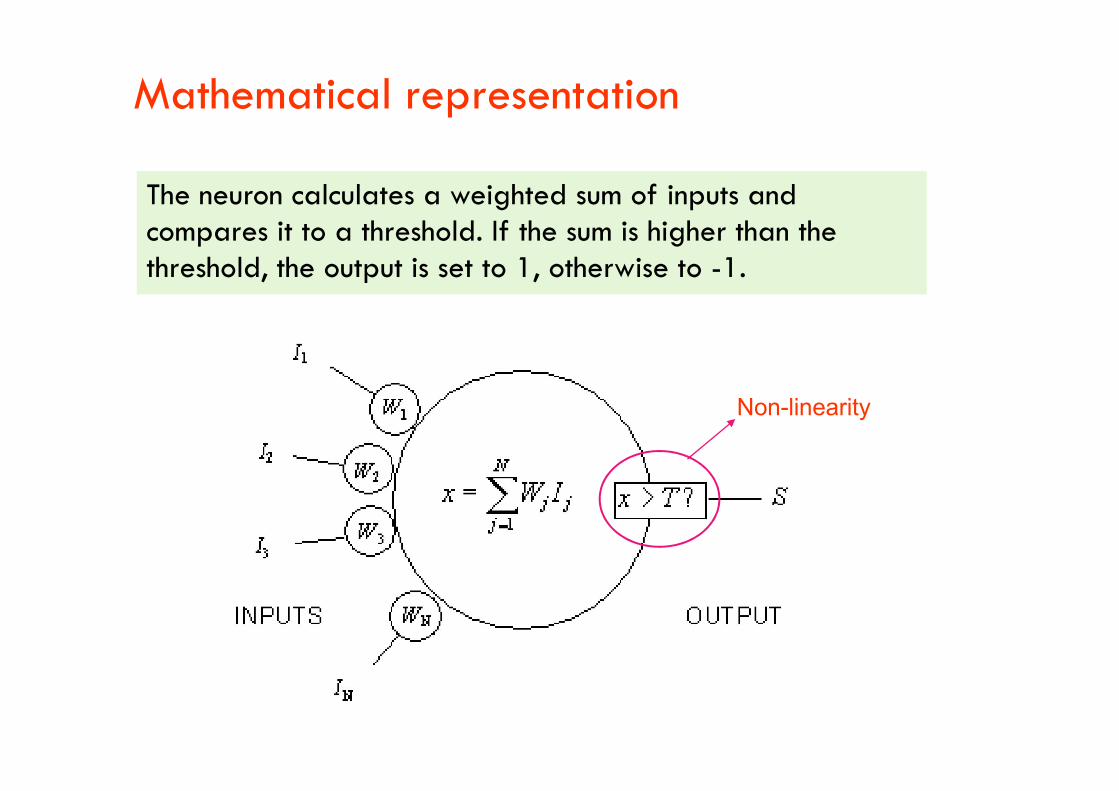
Mathematical representation
The neuron calculates a weighted sum of inputs and compares it to a threshold. If the sum is higher than the threshold, the output is set to 1, otherwise to -1.
Non-linearityNon-linearity

• x1
• x2
• …
• w1
• w2
• …
• wn
• i
n
iiwx
1threshold threshold • f
Artificial neurons
• xn
i
n
iin wxxxxf
121 if,1),...,,(
otherwise,0

Basic Concepts
Визначення вузла:
• елемент, що виконує перетворення
Input 0 Input 1 Input n...
W0 W1 Wn...
y = fH(∑(wixi) + Wb)fH(x)
+
Output
+Wb
NodeNode
ConnectionConnection

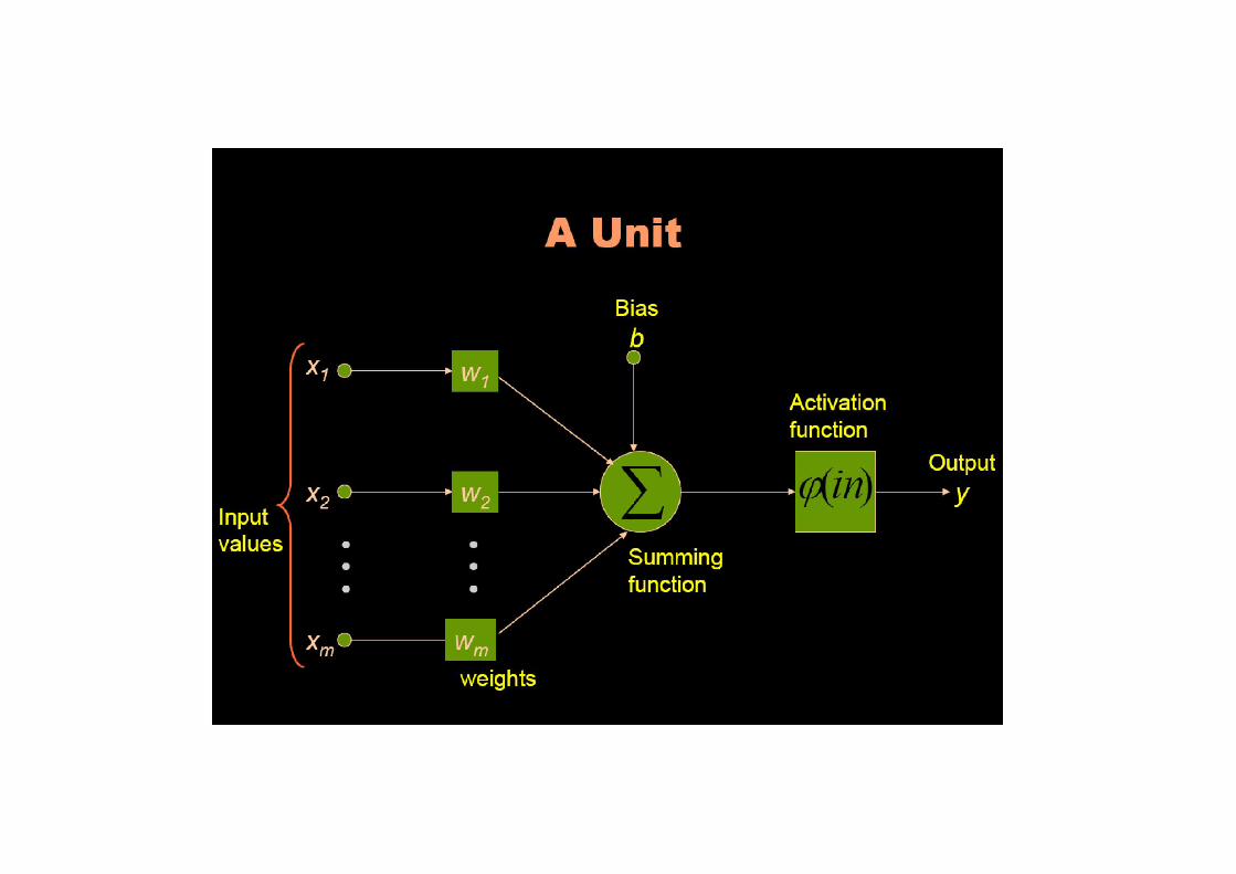
Anatomy of an Artificial Neuron
bias
inputs
x1 w1
1
w0f : activation function
inputs
h(w0,wi , xi ) y f h y
1
xi
wi
xnwn
output
h : combine wi & xi
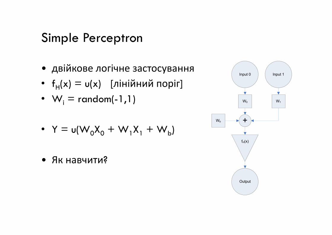
Simple Perceptron
• двійкове логічне застосування
• fH(x) = u(x) [лінійний поріг]
• Wi = random(-1,1)
Input 0 Input 1
W0 W1
• Y = u(W0X0 + W1X1 + Wb)
• Як навчити?
fH(x)
+
Output
Wb

• З досвіду: приклади / навчальні дані
• Сила зв’язків між нейронами зберігається
Artificial Neuron
A physical neuron
зберігається як величина ваги специфічних з’єднань.
• Навчити розв’язувати проблему = зміна ваг з’єднань
An artificial neuron
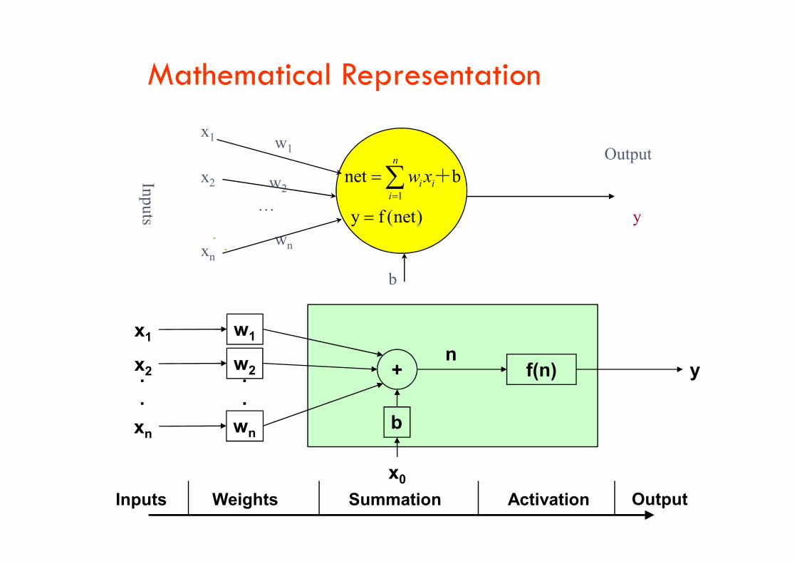
Mathematical Representation
Inputs
Output
w2
w1
wn.
.
… y
1
net b
y f (net)
n
i ii
w x
+x2
xn
b
x1
bw1
w2
wn
x1
x2
xn
+
b
x0
f(n)..
.
.
ny
Inputs Weights Summation Activation Output
b
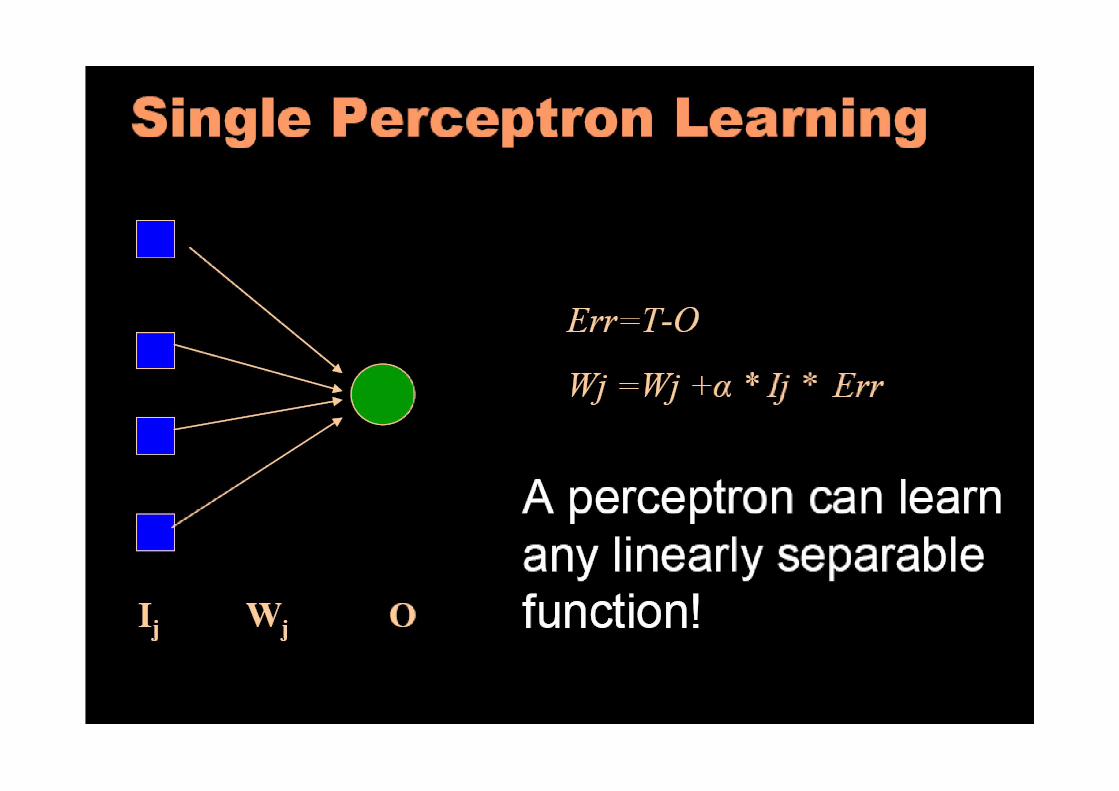

A simple perceptron
• Мережа з єдиним unit
• Змінює ваги на величину, пропорційну різниці між бажаним і фактичним виходом.
Δ Wi = η * (D-Y).Ii
Perceptron Learning Rule
Learning rateDesired output
Input
Actual output

Лінійні нейрони
•Очевидно, той факт, що порогові units можуть виводити тільки значення 0 і 1 обмежує їх застосовність до певних проблем.
•Ми можемо подолати це обмеження, усуваючи поріг і просто замінюючи Fi тотожною функцією, так що ми отримуємо:
)(net )( tto ii )(net )( tto ii
•З такого типу нейронами можемо будувати мережі з m input нейронами і n output нейронами, здатні обчислити:
f: Rm Rn.

Linear Neurons
•Linear neurons are quite popular and useful for applications such as interpolation.
•However, they have a serious limitation: Each neuron computes a linear function, and therefore the overall network function f: Rm Rn is also linear.
•This means that if an input vector x results in an output vector y, then for any factor the input x will result in the output y.any factor the input x will result in the output y.
•Obviously, many interesting functions cannot be realized by networks of linear neurons.
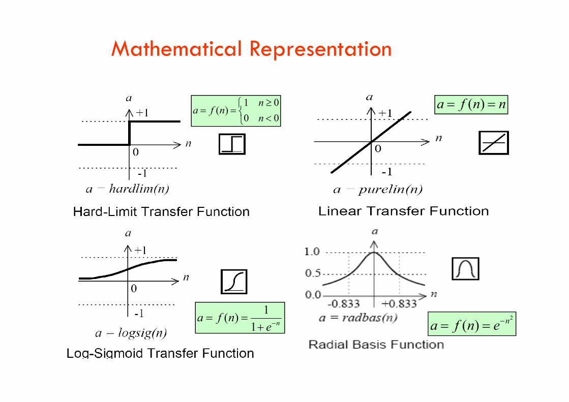
Mathematical Representation
00
01)(
n
nnfa
nnfa )(
nenfa
1
1)( 2
( ) na f n e
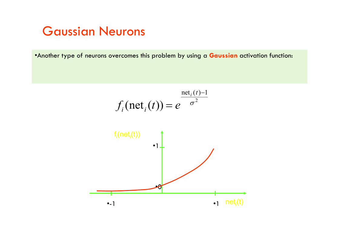
Gaussian Neurons
•Another type of neurons overcomes this problem by using a Gaussian activation function:
2
1)(net
))(net(
t
ii
i
etf
•1
•0
•1
ffii(net(netii(t))(t))
netnetii(t)(t)•-1
Gaussian Neurons
•Gaussian neurons are able to realize non-linear functions.
•Therefore, networks of Gaussian units are in principle unrestricted with regard to the functions that they can realize.
•The drawback of Gaussian neurons is that we have to make sure that their net input does not exceed 1.exceed 1.
•This adds some difficulty to the learning in Gaussian networks.

Sigmoidal Neurons
•Sigmoidal neurons accept any vectors of real numbers as input, and they output a real number between 0 and 1.
•Sigmoidal neurons are the most common type of artificial neuron, especially in learning networks.
•A network of sigmoidal units with m input neurons and n output neurons realizes a network •A network of sigmoidal units with m input neurons and n output neurons realizes a network function f: Rm (0,1)n

Sigmoidal Neurons
•1
ffii(net(netii(t))(t))
/))(net(1
1))(net(
tiiie
tf
• = 1
• = 0.1
•The parameter controls the slope of the sigmoid function, while the parameter controls the horizontal offset of the function in a way similar to the threshold neurons.
•0
•1 netnetii(t)(t)•-1
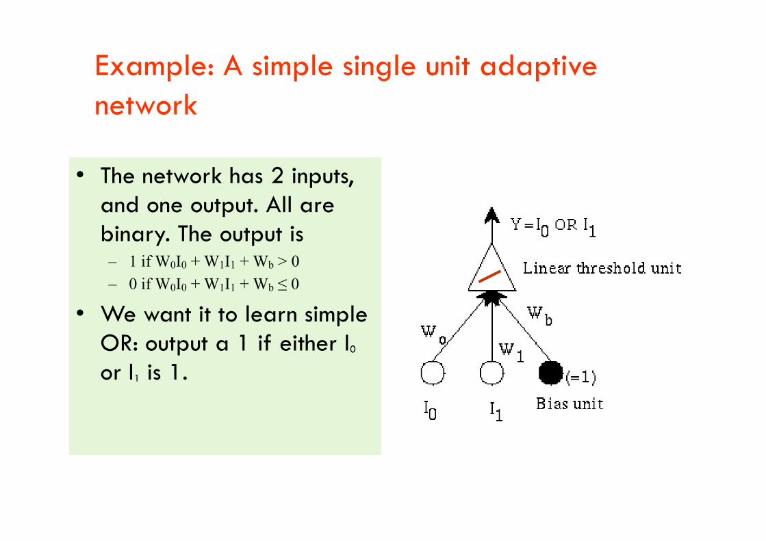
Example: A simple single unit adaptive network
• The network has 2 inputs, and one output. All are binary. The output is – 1 if W0I0 + W1I1 + Wb > 0– 1 if W0I0 + W1I1 + Wb > 0
– 0 if W0I0 + W1I1 + Wb ≤ 0
• We want it to learn simple OR: output a 1 if either I0
or I1 is 1.

Artificial neurons
The McCullogh-Pitts model:
• spikes are interpreted as spike rates;
• synaptic strength are translated as synaptic weights;
• excitation means positive product between the incoming spike rate and the corresponding synaptic weight;
• inhibition means negative product between the incoming spike rate and the corresponding synaptic weight;

Artificial neurons
Nonlinear generalization of the McCullogh-Pitts neuron:
),( wxfy
y is the neuron’s output, x is the vector of inputs, and w is the vector of synaptic weights.y is the neuron’s output, x is the vector of inputs, and w is the vector of synaptic weights.
Examples:
2
2
2
||||
1
1
a
wx
axw
ey
ey
T
sigmoidal neuron
Gaussian neuron

NNs: Dimensions of a Neural Network
– Knowledge about the learning task is given in the form of examples called training examples.
– A NN is specified by:
– an architecture: a set of neurons and links connecting neurons. Each link has a weight,
– a neuron model: the information processing unit of the NN,
– a learning algorithm: used for training the NN by modifying the weights in order to solve the particular learning task correctly on the training examples.solve the particular learning task correctly on the training examples.
The aim is to obtain a NN that generalizes well, that is, that behaves correctly on new instances of the learning task.

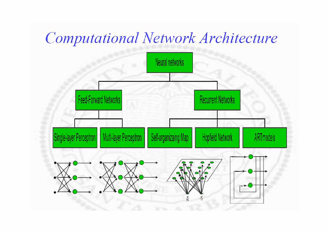
Neural Network Architectures

Neural Network Architectures
Many kinds of structures, main distinction made between two classes:
a) feed- forward (a directed acyclic graph (DAG): links are unidirectional, no cycles
b) recurrent: links form arbitrary topologies e.g., Hopfield Networks and Boltzmann machinesBoltzmann machines
Recurrent networks: can be unstable, or oscillate, or exhibit chaotic
behavior e.g., given some input values, can take a long time to
compute stable output and learning is made more difficult….
However, can implement more complex agent designs and can model
systems with state
We will focus more on feed- forward networks


Single Layer Feed-forward
Input layerof
Output layerof
source nodes
Output layerof
neurons

Multi layer feed-forward
Input Output
3-4-2 Network
Inputlayer
Outputlayer
Hidden Layer
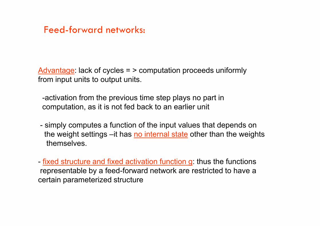
Feed-forward networks:
Advantage: lack of cycles = > computation proceeds uniformly from input units to output units.
-activation from the previous time step plays no part in computation, as it is not fed back to an earlier unit
- simply computes a function of the input values that depends on the weight settings –it has no internal state other than the weightsthemselves.
- fixed structure and fixed activation function g: thus the functionsrepresentable by a feed-forward network are restricted to have acertain parameterized structure

Learning in biological systems
Learning = learning by adaptation
The young animal learns that the green fruits are sour, while the yellowish/reddish ones The young animal learns that the green fruits are sour, while the yellowish/reddish ones are sweet. The learning happens by adapting the fruit picking behavior.
At the neural level the learning happens by changing of the synaptic strengths, eliminating some synapses, and building new ones.

Learning as optimisation
The objective of adapting the responses on the basis of the information received from the environment is to achieve a better state. E.g., the animal likes to eat many energy rich, juicy fruits that make its stomach full, and makes it feel happy.
In other words, the objective of learning in biological organisms is to optimise the amount of available resources, happiness, or in general to achieve a closer to optimal state.

Synapse concept
• The synapse resistance to the incoming signal can be
changed during a "learning" process [1949]
Hebb’s Rule:
If an input of a neuron is repeatedly and persistently causing the neuron to fire, a metabolic change happens in the synapse of that particular
input to reduce its resistance

Neural Network Learning
• Objective of neural network learning: given a set of examples, find parameter settings that minimize the error.
• Programmer specifies• Programmer specifies- numbers of units in each layer - connectivity between units,
• Unknowns- connection weights
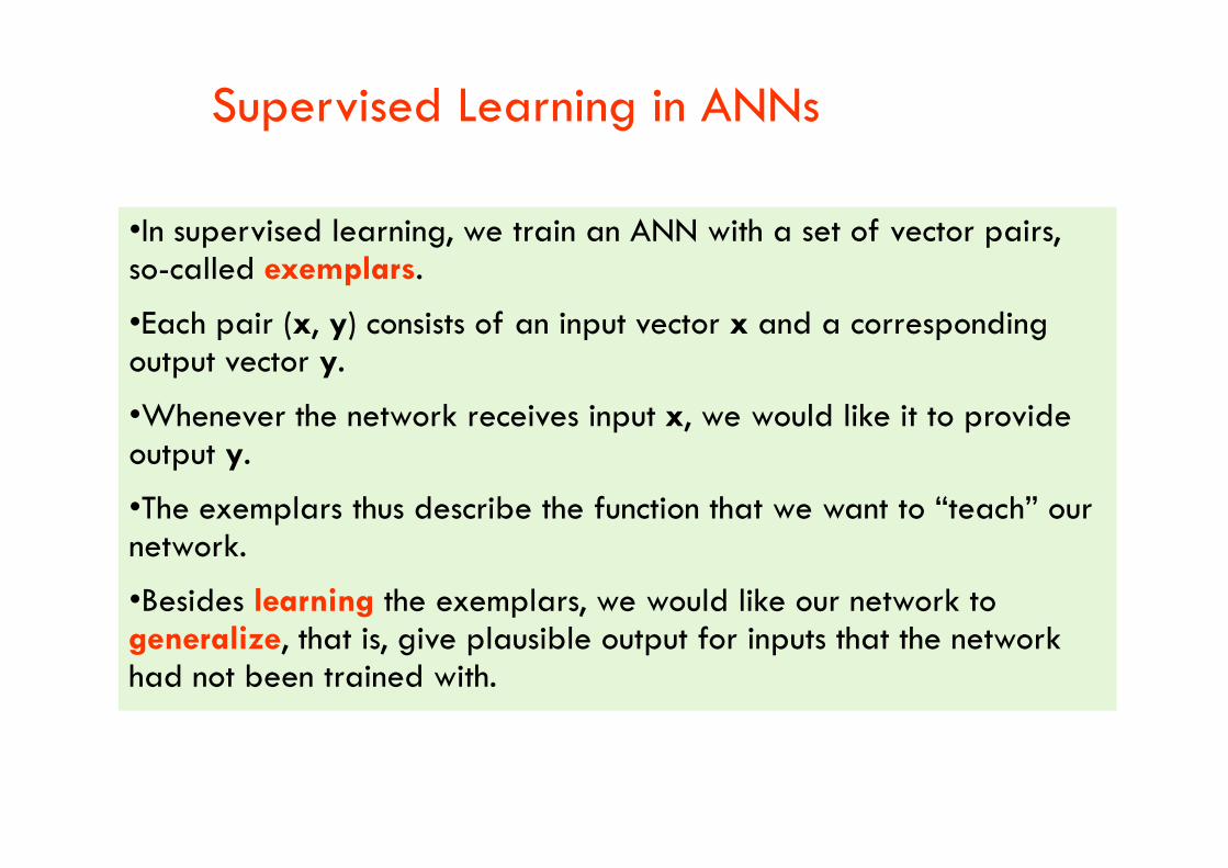
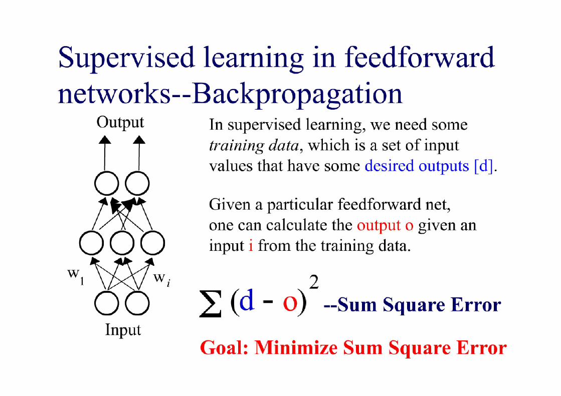
Supervised Learning in ANNs
•In supervised learning, we train an ANN with a set of vector pairs, so-called exemplars.
•Each pair (x, y) consists of an input vector x and a corresponding output vector y.
•Whenever the network receives input x, we would like it to provide output y.•Whenever the network receives input x, we would like it to provide output y.
•The exemplars thus describe the function that we want to “teach” our network.
•Besides learning the exemplars, we would like our network togeneralize, that is, give plausible output for inputs that the network had not been trained with.

Supervised Learning in ANNs
•There is a tradeoff between a network’s ability to precisely learn the given exemplars and its ability to generalize (i.e., inter- and extrapolate).
•This problem is similar to fitting a function to a given set of data points.points.
•Let us assume that you want to find a fitting function f:RR for a set of three data points.
•You try to do this with polynomials of degree one (a straight line), two, and nine.

Supervised Learning in ANNs
•f(x)
•deg. 1
•deg. 2
•deg. 9
•Obviously, the polynomial of degree 2 provides the most plausible fit.
•x
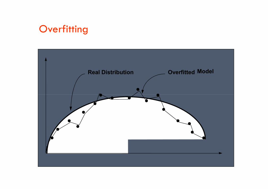
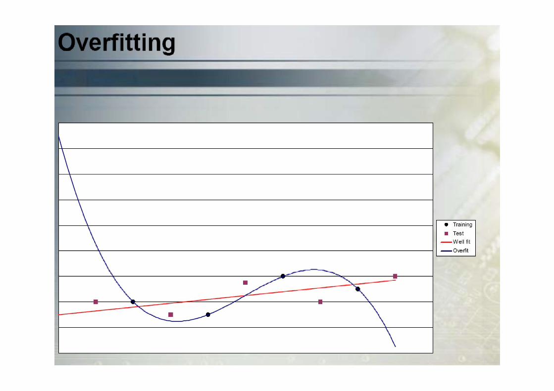
Overfitting
Overfitted ModelReal Distribution
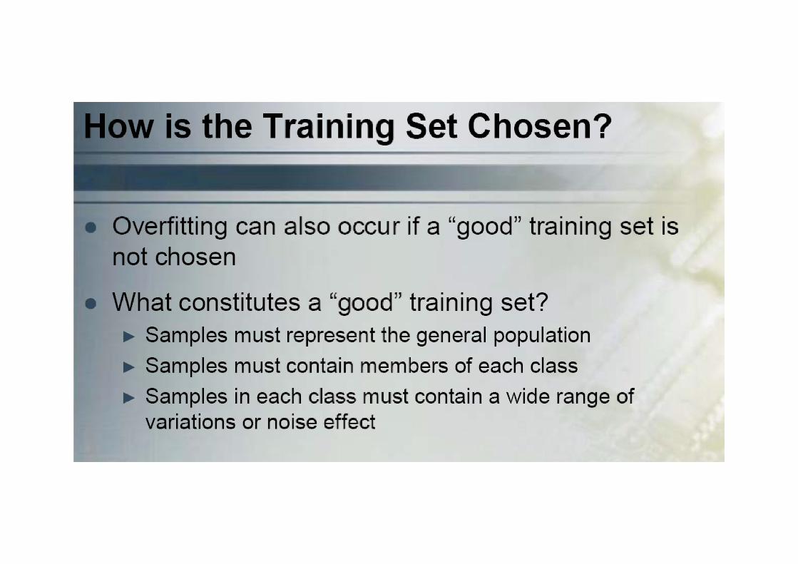


Supervised Learning in ANNs
•The same principle applies to ANNs:
• If an ANN has too few neurons, it may not have enough degrees of freedom to precisely approximate the desired function.
• If an ANN has too many neurons, it will learn the exemplars perfectly, but its additional degrees of
• If an ANN has too many neurons, it will learn the exemplars perfectly, but its additional degrees of freedom may cause it to show implausible behavior for untrained inputs; it then presents poor ability of generalization.
•Unfortunately, there are no known equations that could tell you the optimal size of your network for a given application; you always have to experiment.

Learning in Neural Nets
Learning Tasks
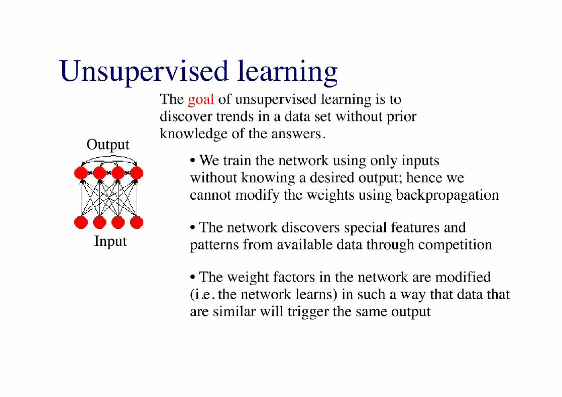
Supervised Unsupervised
Data:Labeled examples(input , desired output)
Tasks:
Data:Unlabeled examples(different realizations of the input)
Tasks:classificationpattern recognition regressionNN models:perceptron adalinefeed-forward NN radial basis functionsupport vector machines
Tasks:clusteringcontent addressable memory
NN models:self-organizing maps (SOM)Hopfield networks

Learning Algorithms
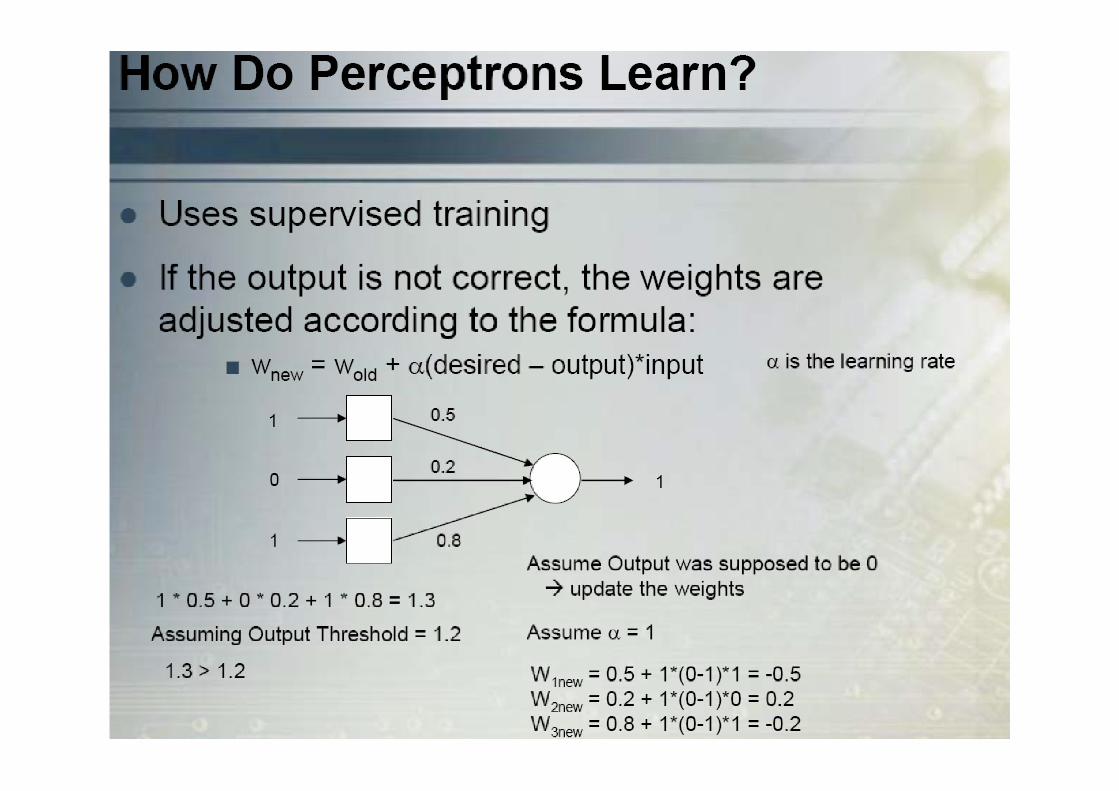
Depend on the network architecture:
• Error correcting learning (perceptron)
• Delta rule (AdaLine, Backprop)• Delta rule (AdaLine, Backprop)
• Competitive Learning (Self Organizing Maps)
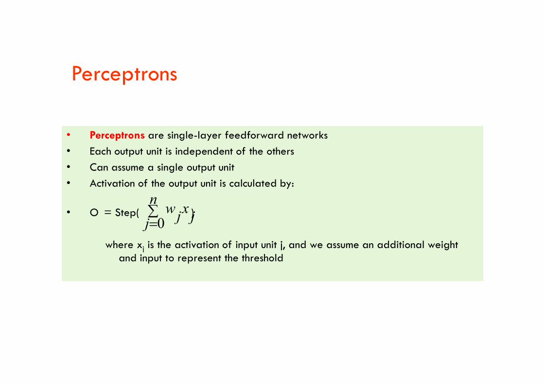
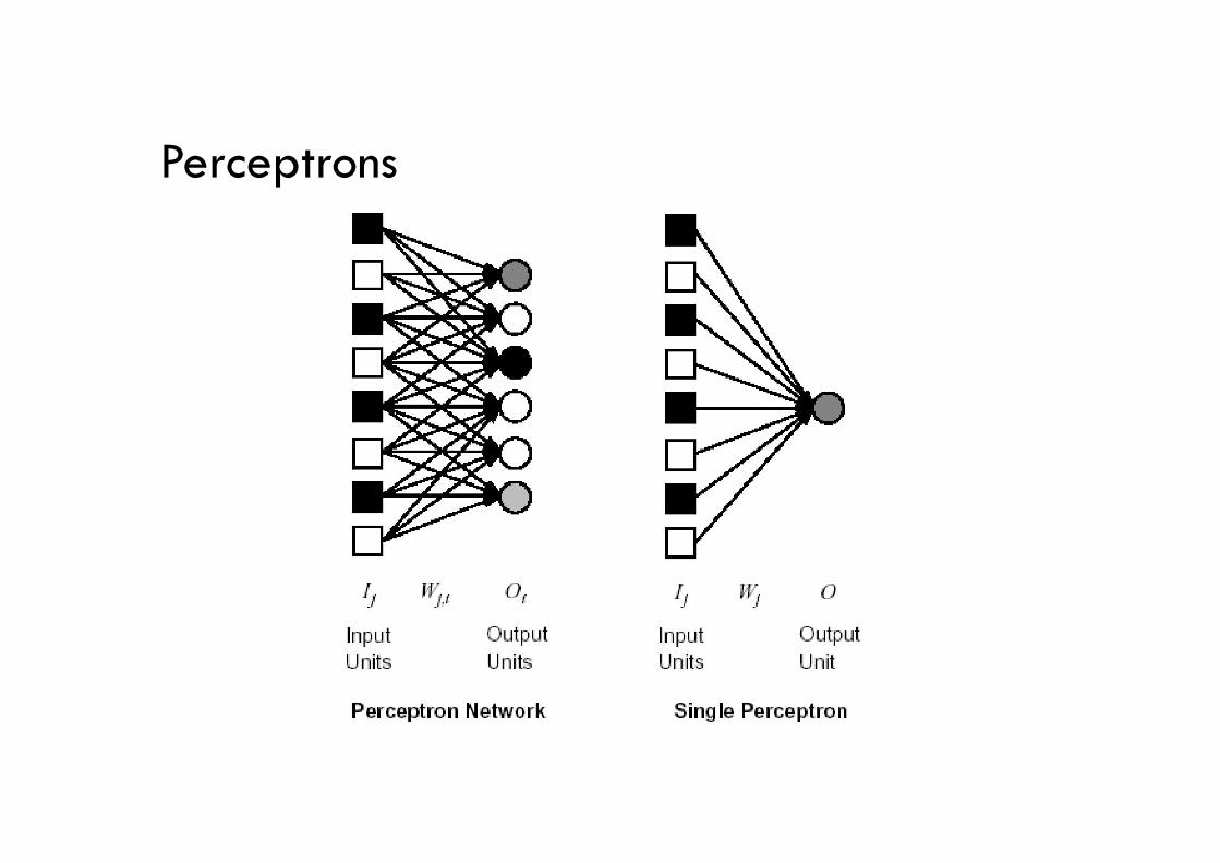
Perceptrons
• Perceptrons are single-layer feedforward networks
• Each output unit is independent of the others
• Can assume a single output unit
• Activation of the output unit is calculated by:
• O = Step( )
where xj is the activation of input unit j, and we assume an additional weight and input to represent the threshold
n
j jx
jw
0

Perceptron
x1
x2w1
w2.
.
X0 = 1
w0
xn wn
.
n
j jx
jw
0 > 01 if
-1 otherwise
O =
n
j jx
jw
0

Perceptron
Rosenblatt (1958) defined a perceptron to be a machine that learns, using examples, to assign input vectors (samples) to different classes, using linear functions of the inputs
Minsky and Papert (1969) instead describe perceptron as a stochastic gradient-descent algorithm that attempts to linearly separate a set of n-dimensional training data.
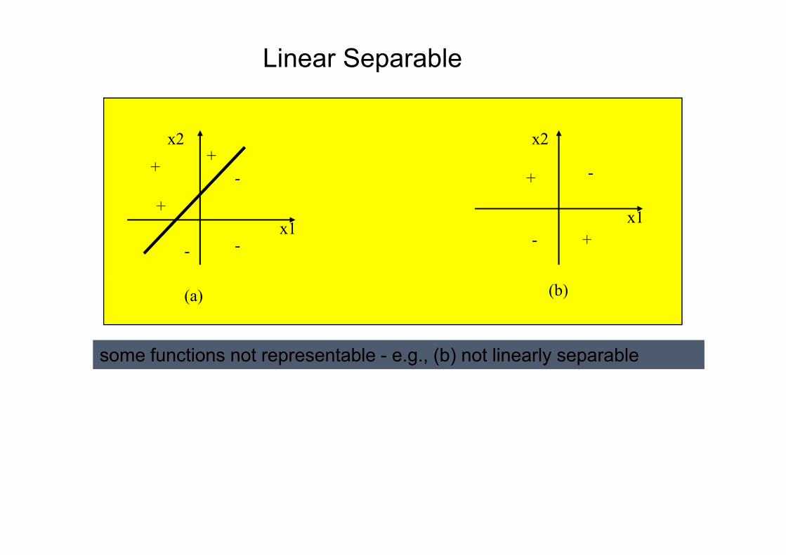
Linear Separable
++
+
-
-
-x1
x2
+
- +
-
x1
x2
(a)
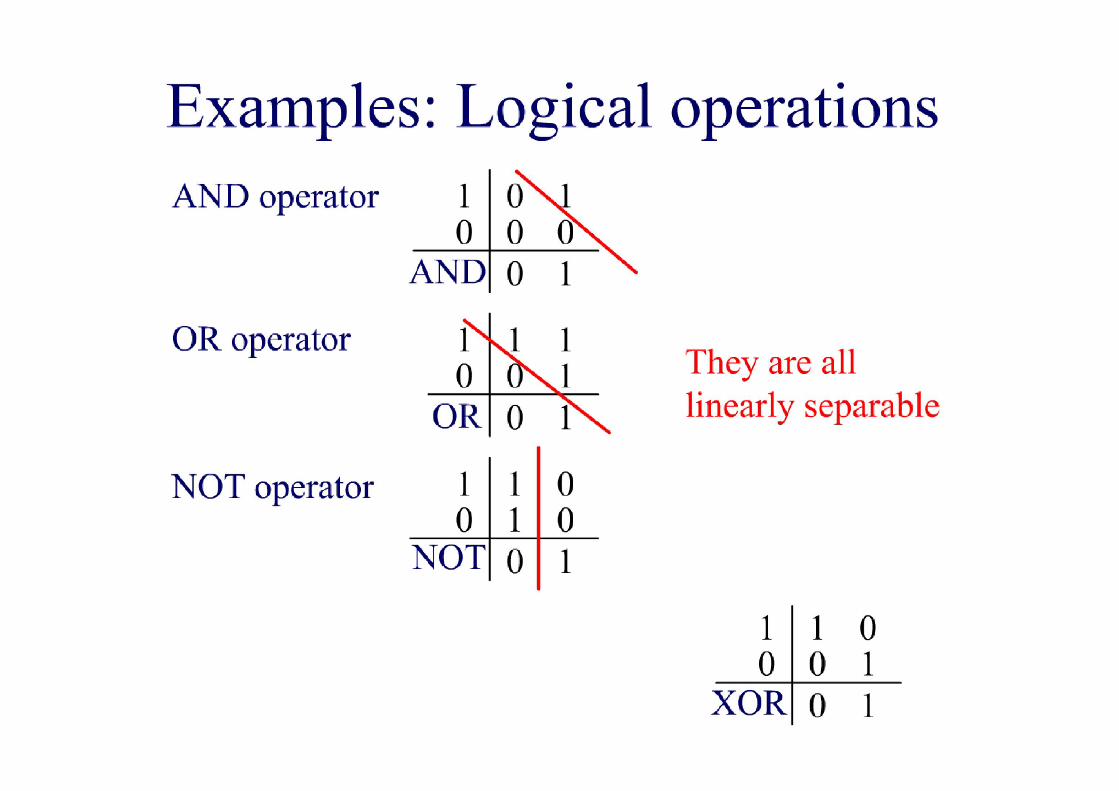
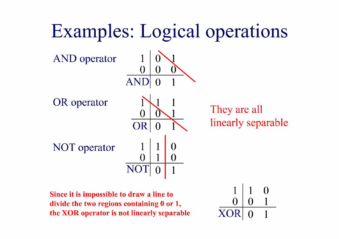
some functions not representable - e.g., (b) not linearly separable
(b)
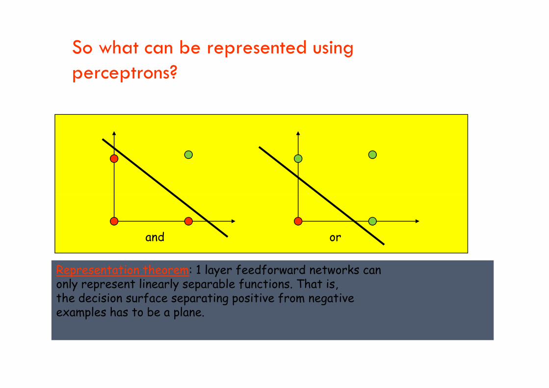
So what can be represented using perceptrons?
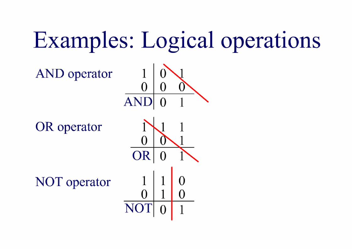
and or
Representation theorem: 1 layer feedforward networks canonly represent linearly separable functions. That is,the decision surface separating positive from negativeexamples has to be a plane.
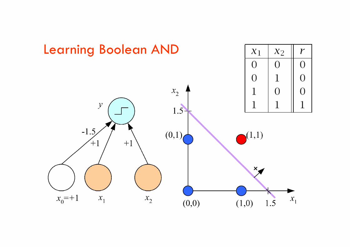
Learning Boolean AND

XOR
• No w0, w1, w2 satisfy:
(Minsky and Papert, 1969)
0
0
0
0
021
01
02
0
www
ww
ww
w
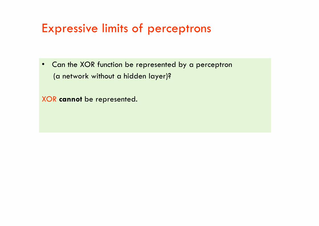
Expressive limits of perceptrons
• Can the XOR function be represented by a perceptron
(a network without a hidden layer)?
XOR cannot be represented.
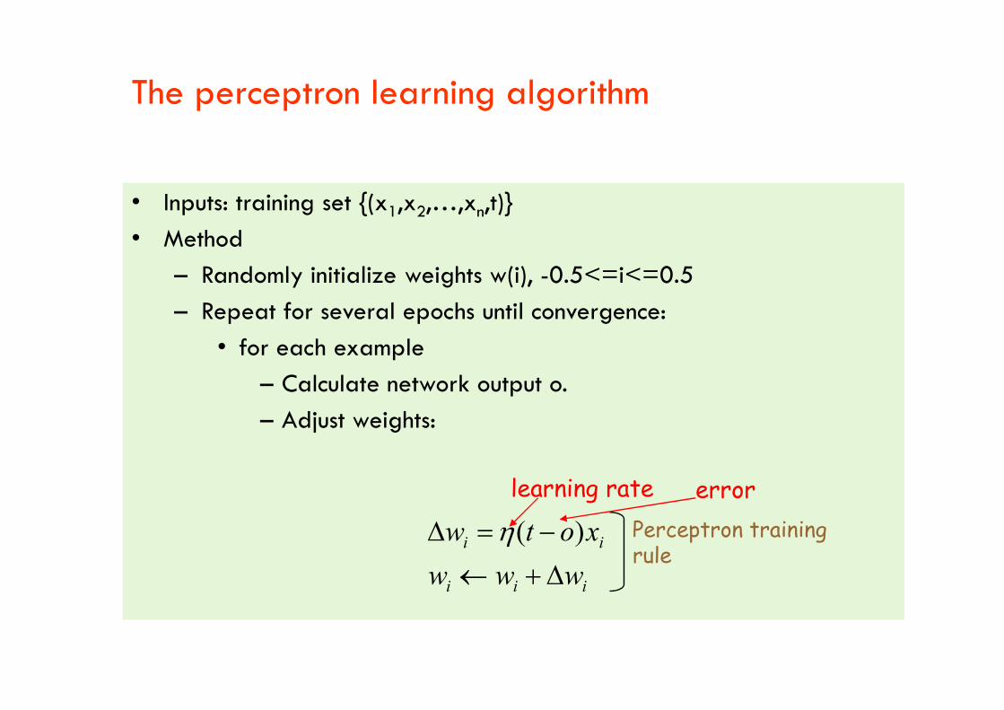
The perceptron learning algorithm
• Inputs: training set {(x1,x2,…,xn,t)}
• Method
– Randomly initialize weights w(i), -0.5<=i<=0.5
– Repeat for several epochs until convergence:
• for each example• for each example
– Calculate network output o.
– Adjust weights:
iii
ii
www
xotw
)( Perceptron trainingrule
learning rate error

Why does the method work?
• The perceptron learning rule performs gradient descent in weight space.
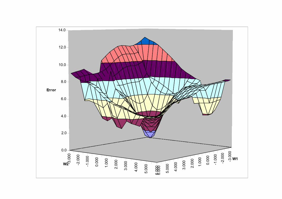
– Error surface: The surface that describes the error on each example as a function of all the weights in the network. A set of weights defines a point on this surface.
– We look at the partial derivative of the surface with respect to each weight (i.e., the gradient -- how much the error would each weight (i.e., the gradient -- how much the error would change if we made a small change in each weight). Then the weights are being altered in an amount proportional to the slope in each direction (corresponding to a weight). Thus the network as a whole is moving in the direction of steepest descent on the error surface.
• The error surface in weight space has a single global minimum and no local minima. Gradient descent is guaranteed to find the global minimum, provided the learning rate is not so big that that you overshoot it.

Multi-layer, feed-forward networks
Perceptrons are rather weak as computing models since they can only learn linearly-separable functions.
Thus, we now focus on multi-layer, feed forward networks of non-linear sigmoid units: i.e., linear sigmoid units: i.e.,
g(x) = xe11
Multi-layer feed-forward networks
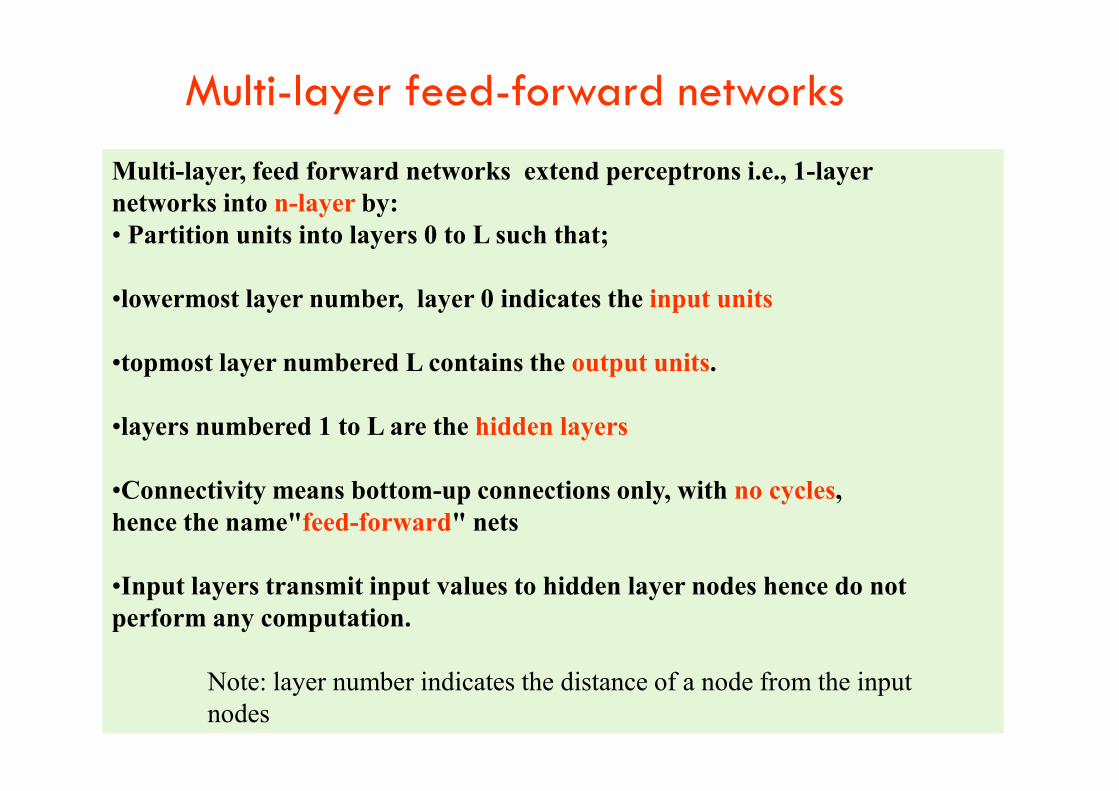
Multi-layer, feed forward networks extend perceptrons i.e., 1-layernetworks into n-layer by:• Partition units into layers 0 to L such that;
•lowermost layer number, layer 0 indicates the input units
•topmost layer numbered L contains the output units.
•layers numbered 1 to L are the hidden layers
•Connectivity means bottom-up connections only, with no cycles, hence the name"feed-forward" nets
•Input layers transmit input values to hidden layer nodes hence do notperform any computation.
Note: layer number indicates the distance of a node from the inputnodes
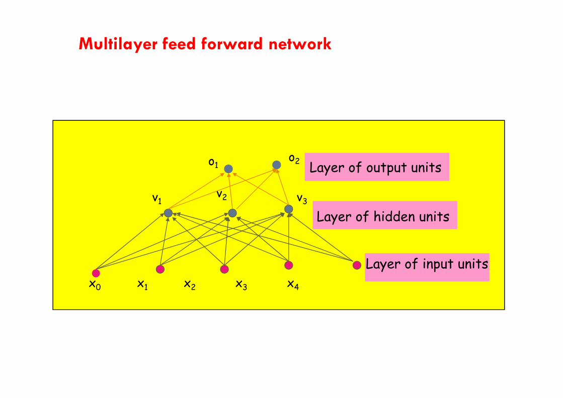
Multilayer feed forward network
v1v2 v3
o1o2
Layer of output units
x0 x1 x2 x3 x4
v1v2 v3
Layer of input units
Layer of hidden units
Multi-layer feed-forward networks
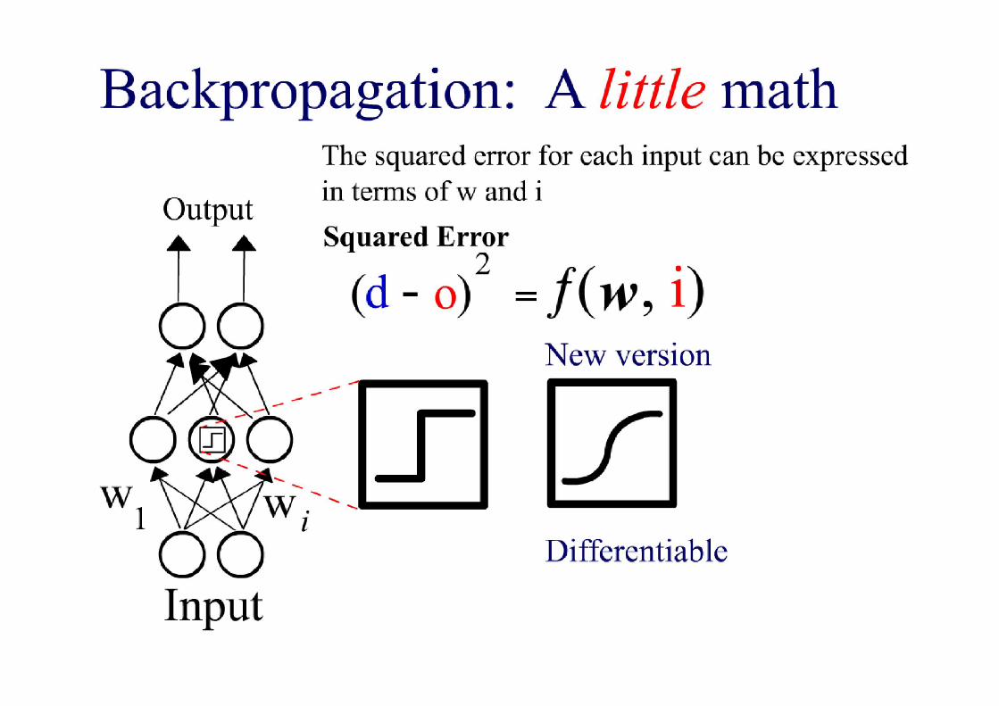
• Multi-layer feed-forward networks can be trained by back-propagationprovided the activation function g is a differentiable function.
– Threshold units don’t qualify, but the sigmoid function does.
• Back-propagation learning is a gradient descent search through the parameter space to minimize the sum-of-squares error. parameter space to minimize the sum-of-squares error.
– Most common algorithm for learning algorithms in multilayer networks
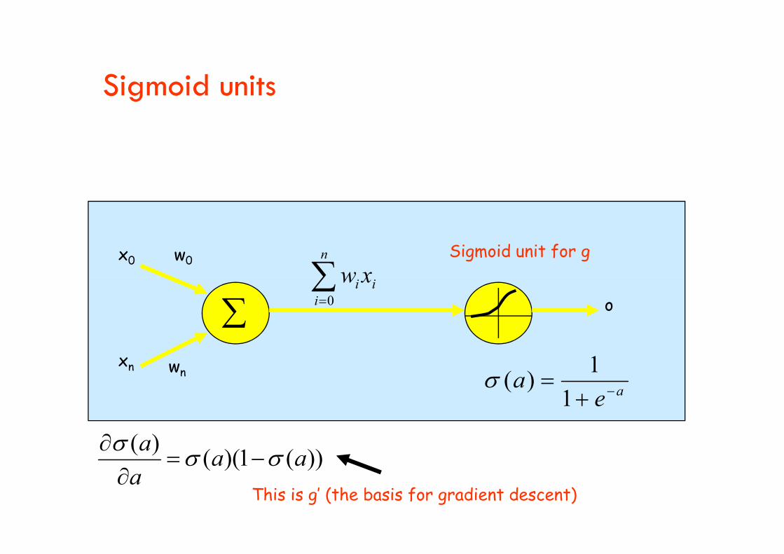
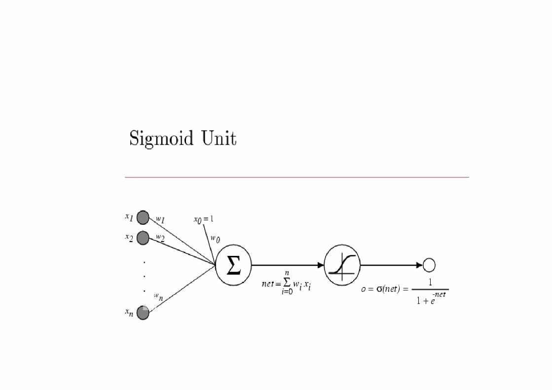
Sigmoid units
x0 w0
i
n
i xwSigmoid unit for g
xn wn
o
ii
i xw0
aea
1
1)(
))(1)(()(
aaa
a
This is g’ (the basis for gradient descent)

Weight updating in backprop
• Learning in backprop is similar to learning with perceptrons, i.e.,
– Example inputs are fed to the network.
• If the network computes an output vector that matches the target, nothing is done.
• If there is a difference between output and target (i.e., an error), then the weights are adjusted to reduce this error.weights are adjusted to reduce this error.
• The key is to assess the blame for the error and divide it among the contributing weights.
• The error term (T - o) is known for the units in the output layer. To adjust the weights between the hidden and the output layer, the gradient descent rule can be applied as done for perceptrons.
• To adjust weights between the input and hidden layer some way of estimating the errors made by the hidden units in needed.

Estimating Error
• Main idea: each hidden node contributes for some fraction of the error in each of the output nodes.
– This fraction equals the strength of the connection (weight) between the hidden node and the output node.
ioutputsi
ijw
j nodehidden at error outputsi
where is the error at output node i.i
A goal of neural network learning is, given a set of examples, to find parameter settings that minimize the error

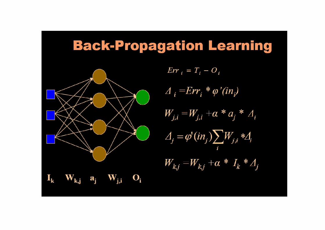
Back-propagation Learning
• Inputs:– Network topology: includes all units & their connections
– Some termination criteria
– Learning Rate (constant of proportionality of gradient descent search) descent search)
– Initial parameter values
– A set of classified training data
• Output: Updated parameter values
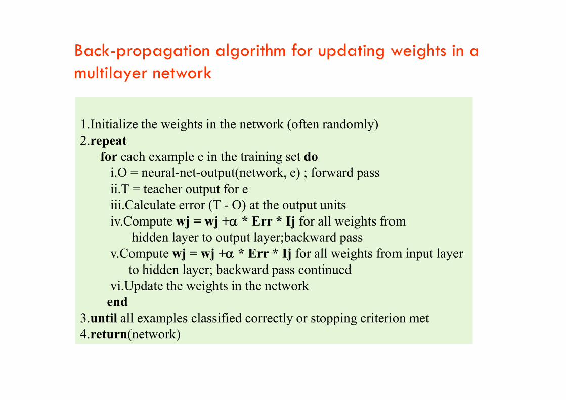
Back-propagation algorithm for updating weights in a multilayer network
1.Initialize the weights in the network (often randomly) 2.repeat
for each example e in the training set doi.O = neural-net-output(network, e) ; forward pass ii.T = teacher output for e iii.Calculate error (T - O) at the output units iii.Calculate error (T - O) at the output units iv.Compute wj = wj +a * Err * Ij for all weights from
hidden layer to output layer;backward pass v.Compute wj = wj +a * Err * Ij for all weights from input layer
to hidden layer; backward pass continued vi.Update the weights in the network
end 3.until all examples classified correctly or stopping criterion met 4.return(network)
Back-propagation Using Gradient Descent
• Advantages– Relatively simple implementation
– Standard method and generally works well
• Disadvantages• Disadvantages– Slow and inefficient
– Can get stuck in local minima resulting in sub-optimal solutions

Number of training pairs needed?
Difficult question. Depends on the problem, the training examples, andnetwork architecture. However, a good rule of thumb is:
epw
Where W = No. of weights; P = No. of training pairs, e = error rate
For example, for e = 0.1, a net with 80 weights will require 800training patterns to be assured of getting 90% of the test patternscorrect (assuming it got 95% of the training examples correct).
How long should a net be trained?
• The objective is to establish a balance between correct responses for the training patterns and correct responses for new patterns. (a balance between memorization and generalization).
• If you train the net for too long, then you run the risk of overfitting.
• In general, the network is trained until it reaches an acceptable error rate (e.g., 95%)

Implementing Backprop – Design Decisions
1. Choice of r2. Network architecture
a) How many Hidden layers? how many hidden units per a layer?b) How should the units be connected? (e.g., Fully, Partial, usingb) How should the units be connected? (e.g., Fully, Partial, using
domain knowledge3. Stopping criterion – when should training stop?
Determining optimal network structure
Weak point of fixed structure networks: poor choice can lead to poor performance
Too small network: model incapable of representing the desired Function
Too big a network: will be able to memorize all examples but forming a large lookup table, but will not generalize well to inputs that have not been seen lookup table, but will not generalize well to inputs that have not been seen before.
Thus finding a good network structure is another example of asearch problems.Some approaches to search for a solution for this problem includeGenetic algorithmsBut using GAs is very cpu-intensive.
Learning rate
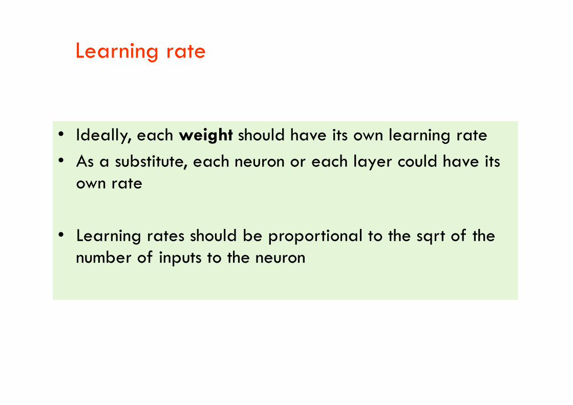
• Ideally, each weight should have its own learning rate
• As a substitute, each neuron or each layer could have its own rate
• Learning rates should be proportional to the sqrt of the number of inputs to the neuron

Setting the parameter values
• How are the weights initialized?
• Do weights change after the presentation of each pattern or only after all patterns of the training set have been presented?
• How is the value of the learning rate chosen?
• When should training stop?
• How many hidden layers and how many nodes in each hidden layer should be chosen to build a feedforward network for a given should be chosen to build a feedforward network for a given problem?
• How many patterns should there be in a training set?
• How does one know that the network has learnt something useful?

When should neural nets be used for learning a problem
• If instances are given as attribute-value pairs.
– Pre-processing required: Continuous input values to be scaled in [0-1] range, and discrete values to be scaled in [0-1] range, and discrete values need to converted to Boolean features.
• Noise in training examples.
• If long training time is acceptable.

Neural Networks: Advantages
•Distributed representations
•Simple computations
•Robust with respect to noisy data
•Robust with respect to node failure •Robust with respect to node failure
•Empirically shown to work well for many problem domains
•Parallel processing
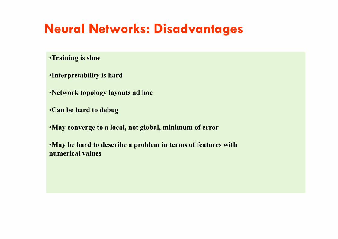
Neural Networks: Disadvantages
•Training is slow
•Interpretability is hard
•Network topology layouts ad hoc
•Can be hard to debug
•May converge to a local, not global, minimum of error
•May be hard to describe a problem in terms of features with numerical values
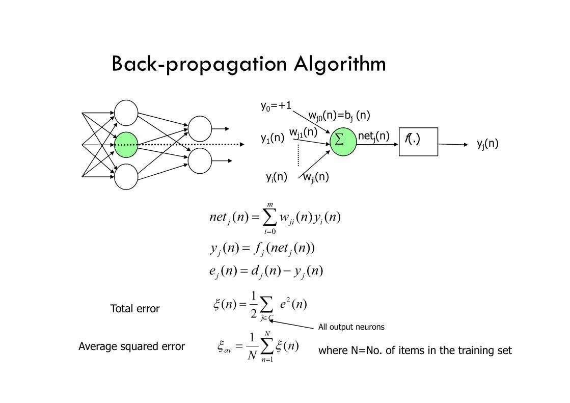
Back-propagation Algorithm
yj(n)
y0=+1
y1(n)
yi(n) wji(n)
wj1(n)
wj0(n)=bj (n)
∑ netj(n) f(.)
m
0
( ) ( ) ( )
( ) ( ( ))
( ) ( ) ( )
m
j ji ii
j j j
j j j
net n w n y n
y n f net n
e n d n y n
Total error )(2
1)( 2 nen
Cj
All output neurons
N
nav n
N 1
)(1
Average squared error where N=No. of items in the training set

( ) ( ) ( )( ) ( )
( ) ( ) ( ) ( ) ( )
j j j
ji j j j ji
e n y n net nn n
w n e n y n net n w n
)()(
)(ne
ne
nj
j
as
1)(
)(
ny
ne
j
j
as
( )' ( ( ))
( )
j
j j
j
y nf net n
net n
as
( )( )
( )
j
i
ji
net ny n
w n
as
Back-propagation Algorithm
( )( ) ( ( )) ( )
( )j j j i
ji
ne n v n y n
w n
)(2
1)( 2 nen
Cj
as as
)()()( nyndne jjj
as
( ) ( ( ))j j jy n f net n
as
0
( ) ( ) ( )m
j ji ii
net n w n y n
Gradient decent
)()()( nynnw ijji
Error term
where ( ) ( ) '( ( ))j j jn e n f net n
)()()( nynnw ijji 1
( ( ))1 exp( ( ))
j j
j
net nnet n
if
as
'( ( )) ( )[1 ( )]j j jnet n y n y n
( ) ( ( ))j j jy n net n

Back-propagation Algorithm
Neuron k is an output node
( ) ( ) '( ( )) [ ( ) ( )] ( )[1 ( )]k k k k k k kn e n net n d n y n y n y n
( ) '( ( )) ( ) ( )
( )[1 ( )] ( ) ( )
j j k kjk
j j k kj
n net n n w n
y n y n n w n
Neuron j is a hidden node Output of neuron k
j j k kjk
Output layer (k)Hidden layer(j)
1
2
jw1
jw2
j
)()()( nynnw ijji
Weight adjustment
Learningrate
Localgradient
Input signal
( 1) ( ) ( )ji ji jiw n w n w n

6.0
8.0
10.0
12.0
14.0
Error
-3.0
00
-2.0
00
-1.0
00
0.0
00
1.0
00
2.0
00
3.0
00
4.0
00
5.0
00
6.0
00
-3.0
00
-2.0
00
-1.0
00
0.0
00
1.0
00
2.0
00
3.0
00
4.0
00
5.0
00
6.0
00
0.0
2.0
4.0
6.0
W1
W2
Inputs
NodeConnection
Outputs
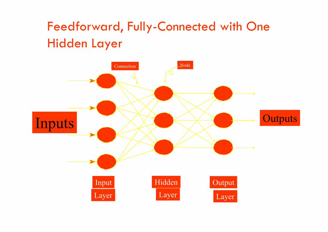
Feedforward, Fully-Connected with One Hidden Layer
Input
Layer
Hidden
Layer
Output
Layer
Inputs Outputs
Hidden Units
• Layer of nodes between input and output nodes
• Allow a network to learn non-linear functions• Allow a network to learn non-linear functions
• Allow the net to represent combinations of the input features

Learning Algorithms
• How the network learns the relationship between the inputs and outputs
• Type of algorithm used depends on type of network- architecture, type of learning,etc.network- architecture, type of learning,etc.
• Back Propagation: most popular– modifications exist: quick prop, Delta-bar-Delta
• Others: Conjugate gradient descent, Levenberg-Marquardt, K-Means, Kohonen, standard pseudo-inverse (SVD) linear optimization
Types of Networks
• Multilayer Perceptron
• Radial Basis Function
• Kohonen
• Linear• Linear
• Hopfield
• Adaline/Madaline
• Probabilistic Neural Network (PNN)
• General Regression Neural Network (GRNN)
• and at least thirty others
Perceptrons
• First studied in the late 1950s
• Also known as Layered Feed-Forward Networks
• The only efficient learning element at that time was for single-layered networksfor single-layered networks
• Today, used as a synonym for a single-layer, feed-forward network
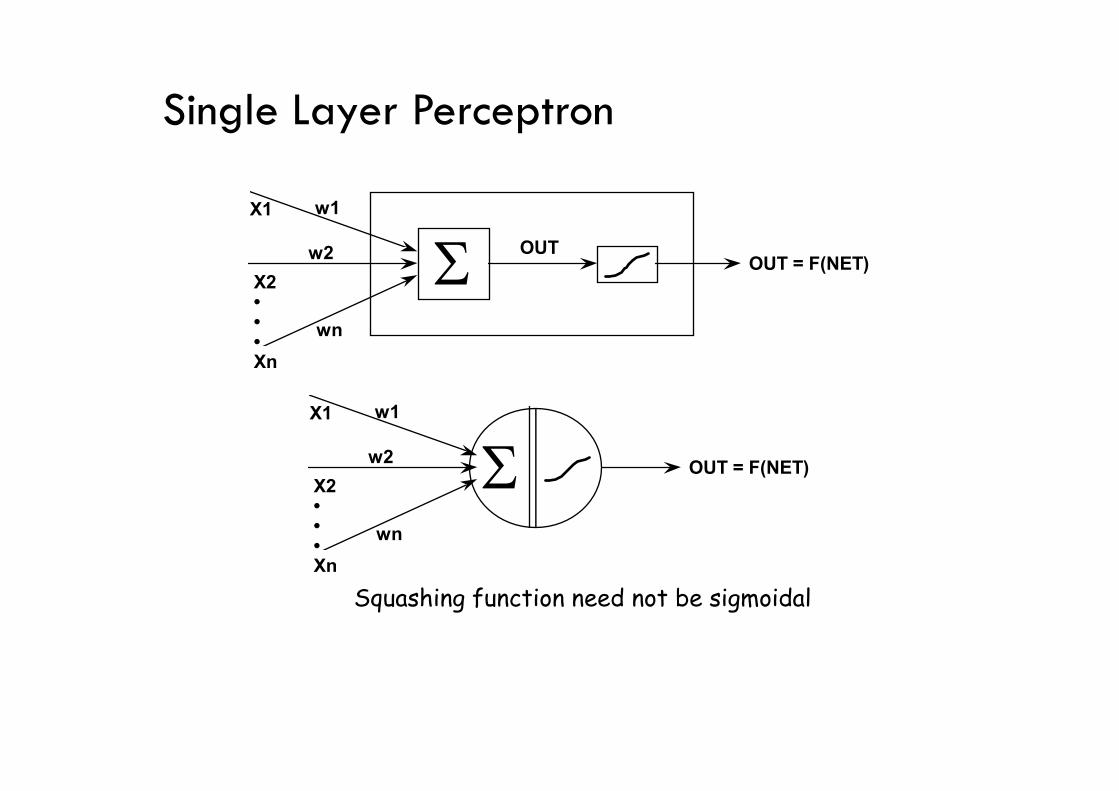
Single Layer Perceptron
OUT = F(NET)OUT
X1
X2 • • • Xn
w1
w2
wn
OUT = F(NET)
X1
X2 • • • Xn
w1
w2
wn
Squashing function need not be sigmoidal

Perceptron Architecture
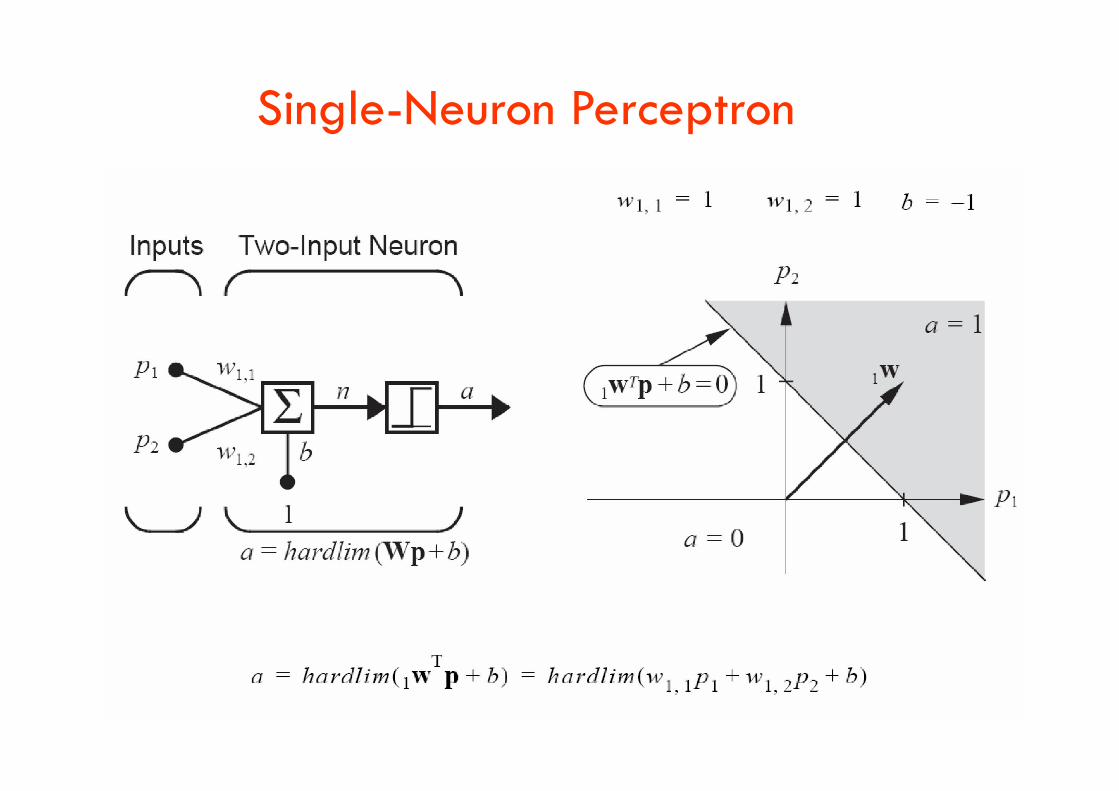
Single-Neuron Perceptron

Decision Boundary
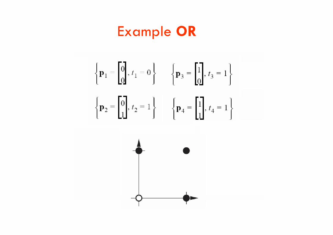
Example OR
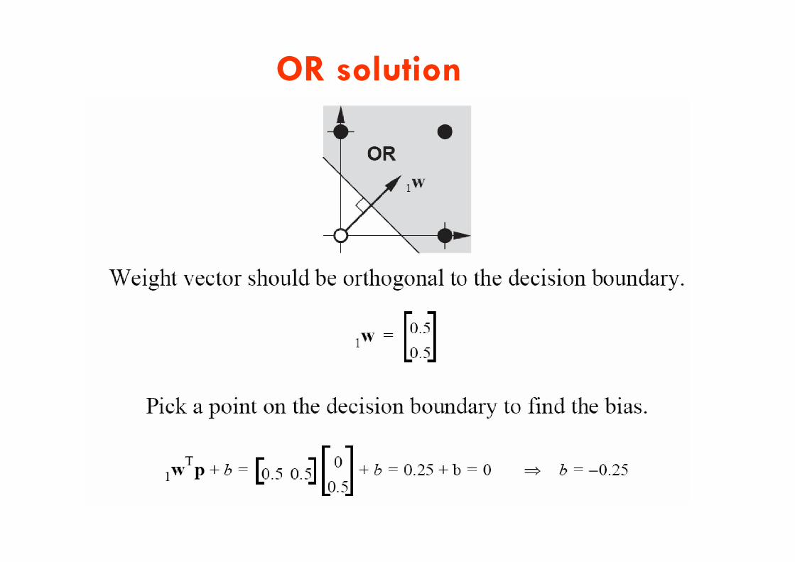
OR solution

Multiple-Neuron Perceptron
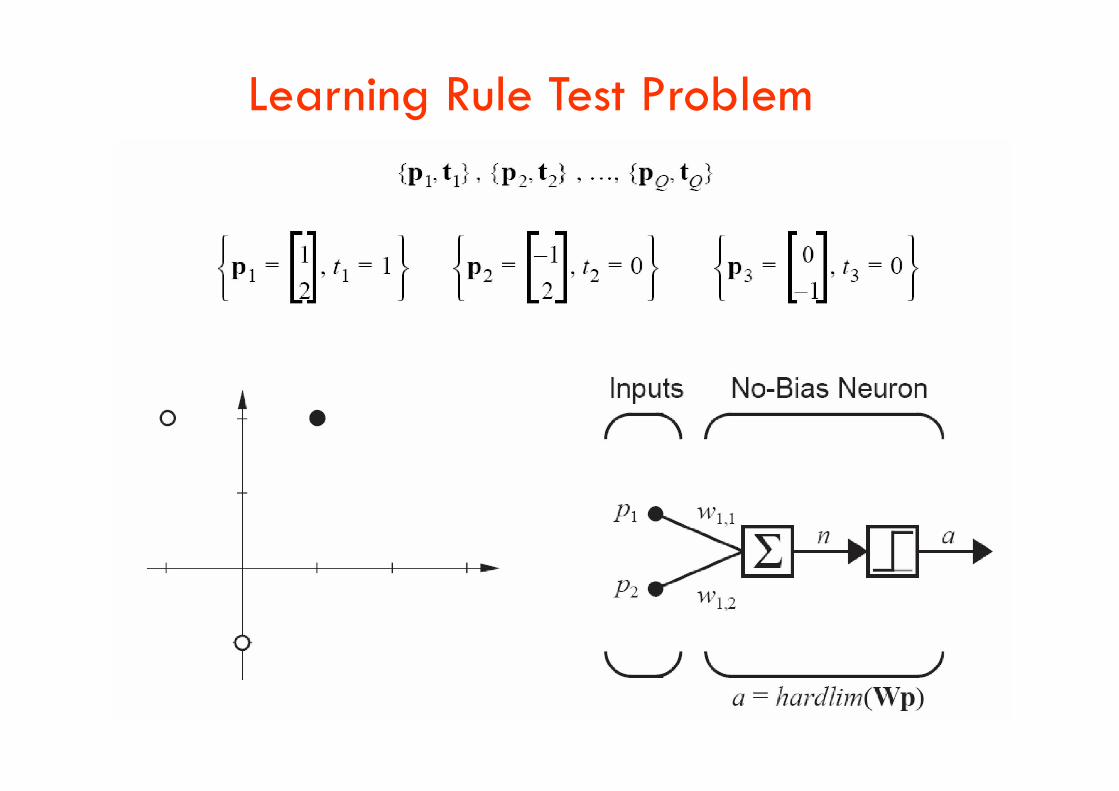
Learning Rule Test Problem

Starting Point
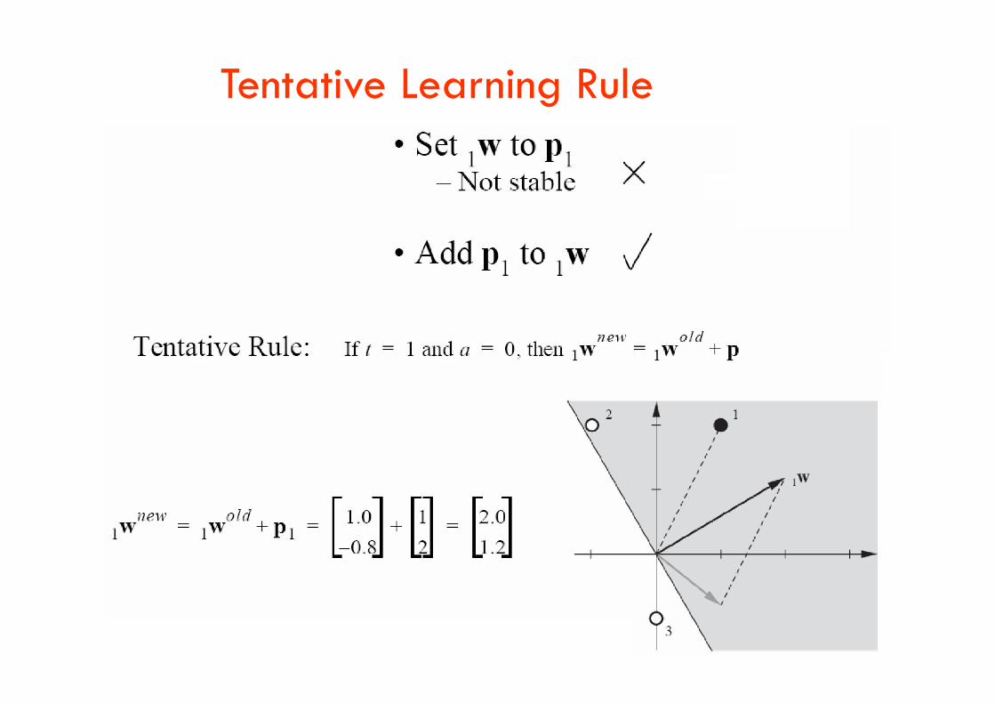
Tentative Learning Rule

Second Input Vector

Third Input Vector
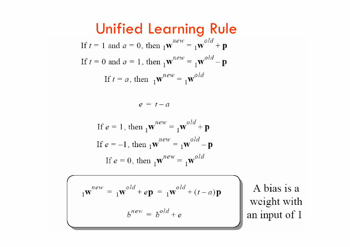
Unified Learning Rule

Multiple-Neuron Perceptron

Apple / Banana Example

Apple / Banana Example, Second iteration

Apple / Banana Example, Check

Multilayer Perceptron(MLP)
• Type of Back Propagation Network
• Arguably the most popular network architecture today
• Can model functions of almost arbitrary complexity, with number of layers and number of units/layer determining number of layers and number of units/layer determining the function complexity
• Number of hidden layers and units: good starting point is to use one hidden layer with the number of units equal to half the sum of the number of input and output units
Perceptrons

Network Structures
Feed-forward:
Links can only go in one direction.
Recurrent :
Links can go anywhere and form arbitrary
topologies.
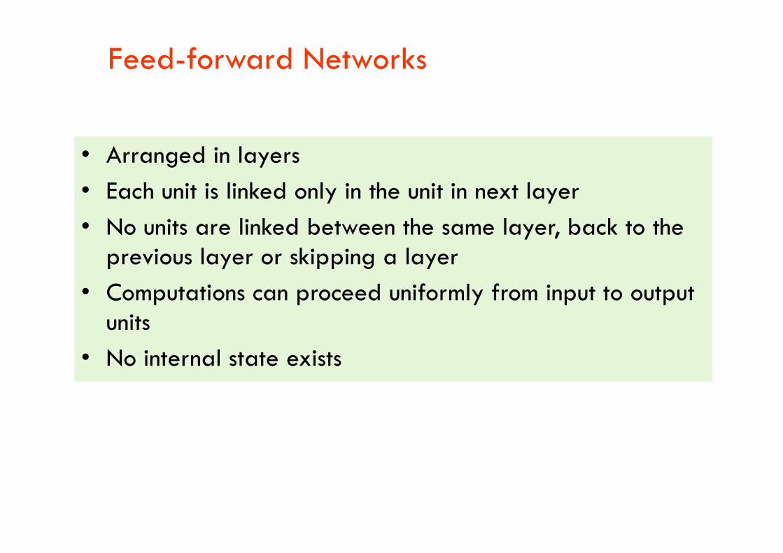
Feed-forward Networks
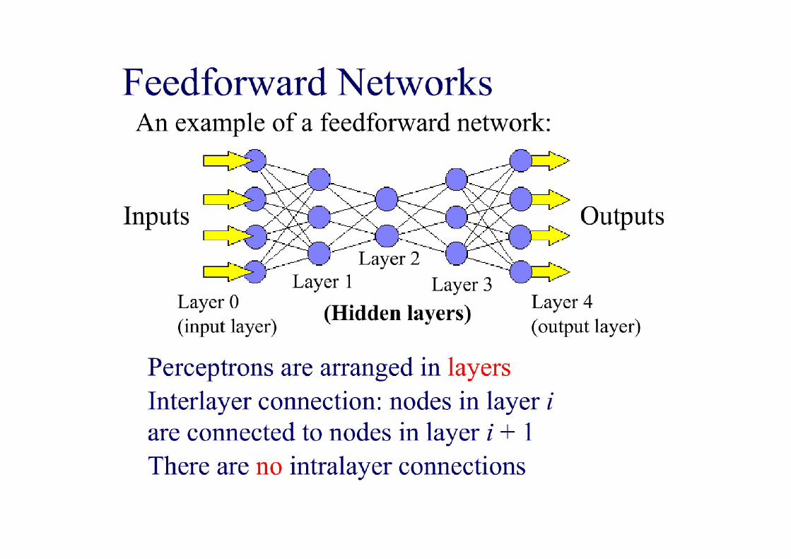
• Arranged in layers
• Each unit is linked only in the unit in next layer
• No units are linked between the same layer, back to the previous layer or skipping a layer
• Computations can proceed uniformly from input to output units
• No internal state exists
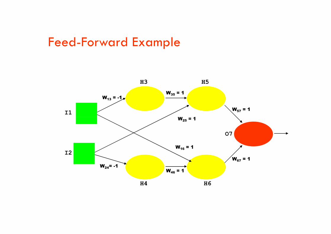
I1
W13 = -1
H3
W35 = 1
H5
W57 = 1
W = 1
Feed-Forward Example
I2
W24= -1
H4
W46 = 1
H6
W67 = 1
O7
W25 = 1
W16 = 1

Introduction to Backpropagation
• In 1969 a method for learning in multi-layer network, Backpropagation, was invented by Bryson and Ho
• The Backpropagation algorithm is a sensible approach for dividing the contribution of each weightfor dividing the contribution of each weight
• Works basically the same as perceptrons
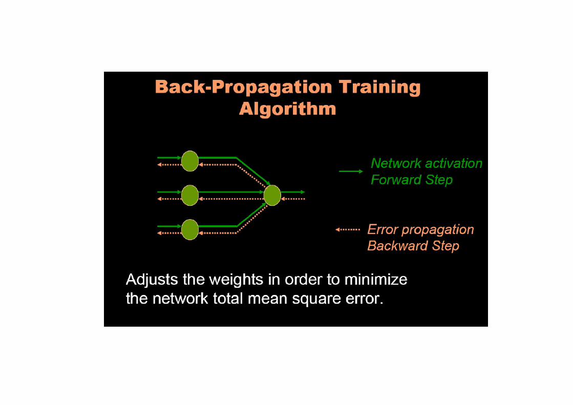


Backpropagation Learning
• There are two differences for the updating rule :– The activation of the hidden unit is used instead of the
input valueinput value
– The rule contains a term for the gradient of the activation function

Backpropagation Algorithm Summary
The ideas of the algorithm can be summarized as follows :
• Computes the error term for the output units using the observed error
• From output layer, repeat propagating the error term • From output layer, repeat propagating the error term back to the previous layer and updating the weights between the two layers until the earliest hidden layer is reached

Back Propagation
• Best-known example of a training algorithm
• Uses training data to adjust weights and thresholds of neurons so as to minimize the networks errors of prediction
• Slower than modern second-order algorithms such as gradient descent & Levenberg-Marquardt for many problemsdescent & Levenberg-Marquardt for many problems
• Still has some advantages over these in some instances
• Easiest algorithm to understand
• Heuristic modifications exist: quick propagation and Delta-bar-Delta

Training a BackPropagation Net
• Feedforward training of input patterns– each input node receives a signal, which is broadcast to all of the hidden units
– each hidden unit computes its activation which is broadcast to all output nodes
• Back propagation of errors– each output node compares its activation with the desired output
– based on these differences, the error is propagated back to all previous nodes
• Adjustment of weights• Adjustment of weights– weights of all links computed simultaneously based on the errors that were propagated
back

Training Back Prop Net: Feedforward Stage
1. Initialize weights with small, random values
2. While stopping condition is not true– for each training pair (input/output):
• each input unit broadcasts its value to all hidden units• each input unit broadcasts its value to all hidden units
• each hidden unit sums its input signals & applies activation function to compute its output signal
• each hidden unit sends its signal to the output units
• each output unit sums its input signals & applies its activation function to compute its output signal

Training Back Prop Net: Backpropagation
3. Each output computes its error term, its own weight correction term and its bias(threshold) correction term & sends it to layer below
4. Each hidden unit sums its delta inputs from above & 4. Each hidden unit sums its delta inputs from above & multiplies by the derivative of its activation function; it also computes its own weight correction term and its bias correction term

Training a Back Prop Net: Adjusting the Weights
5. Each output unit updates its weights and bias
6. Each hidden unit updates its weights and bias– Each training cycle is called an epoch. The weights are updated in each cycle
– It is not analytically possible to determine where the global minimum is. Eventually the algorithm stops in a low point, which may just be a local Eventually the algorithm stops in a low point, which may just be a local minimum.
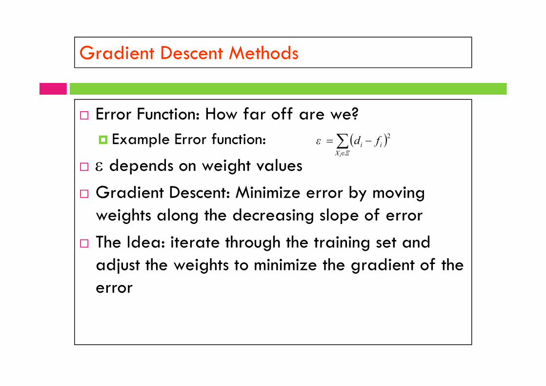
Gradient Descent Methods
Error Function: How far off are we?
Example Error function:
depends on weight values
Gradient Descent: Minimize error by moving
ΞΧ
ii
i
fdε2
Gradient Descent: Minimize error by moving weights along the decreasing slope of error
The Idea: iterate through the training set and adjust the weights to minimize the gradient of the error

Gradient Descent: The Math
We have = (d - f)2
Gradient of :
Using the chain rule:
11
,...,,...,ni wwwW
W
s
sW
Using the chain rule:
Since , we have
Also:
Which finally gives:
WsW
W
s
sW
s
ffd
s
)(2
s
ffd
W)(2
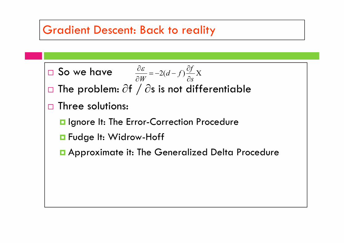
Gradient Descent: Back to reality
So we have
The problem: f / s is not differentiable
Three solutions:
Ignore It: The Error-Correction Procedure
s
ffd
W)(2
Ignore It: The Error-Correction Procedure
Fudge It: Widrow-Hoff
Approximate it: The Generalized Delta Procedure

Training a Back Prop Net: Adjusting the Weights
5. Each output unit updates its weights and bias
6. Each hidden unit updates its weights and bias– Each training cycle is called an epoch. The weights are updated in each cycle
– It is not analytically possible to determine where the global minimum is. Eventually the algorithm stops in a low point, which may just be a local minimum.
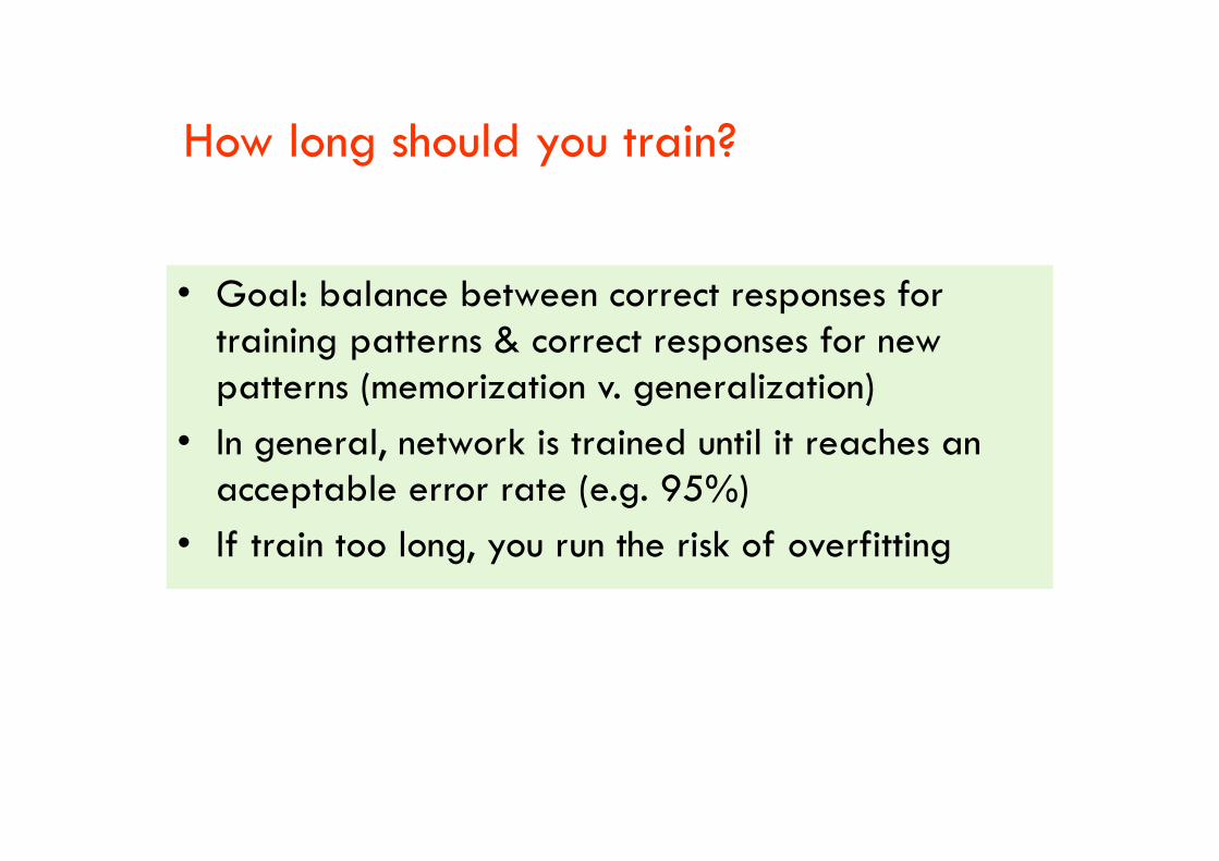
How long should you train?
• Goal: balance between correct responses for training patterns & correct responses for new patterns (memorization v. generalization)
• In general, network is trained until it reaches an • In general, network is trained until it reaches an acceptable error rate (e.g. 95%)
• If train too long, you run the risk of overfitting

Learning in the BPN
•Before the learning process starts, all weights (synapses) in the network areinitialized with pseudorandom numbers.
•We also have to provide a set of training patterns (exemplars). They can be described as a set of ordered vector pairs {(x1, y1), (x2, y2), …, (xP, yP)}.
•Then we can start the backpropagation learning algorithm.
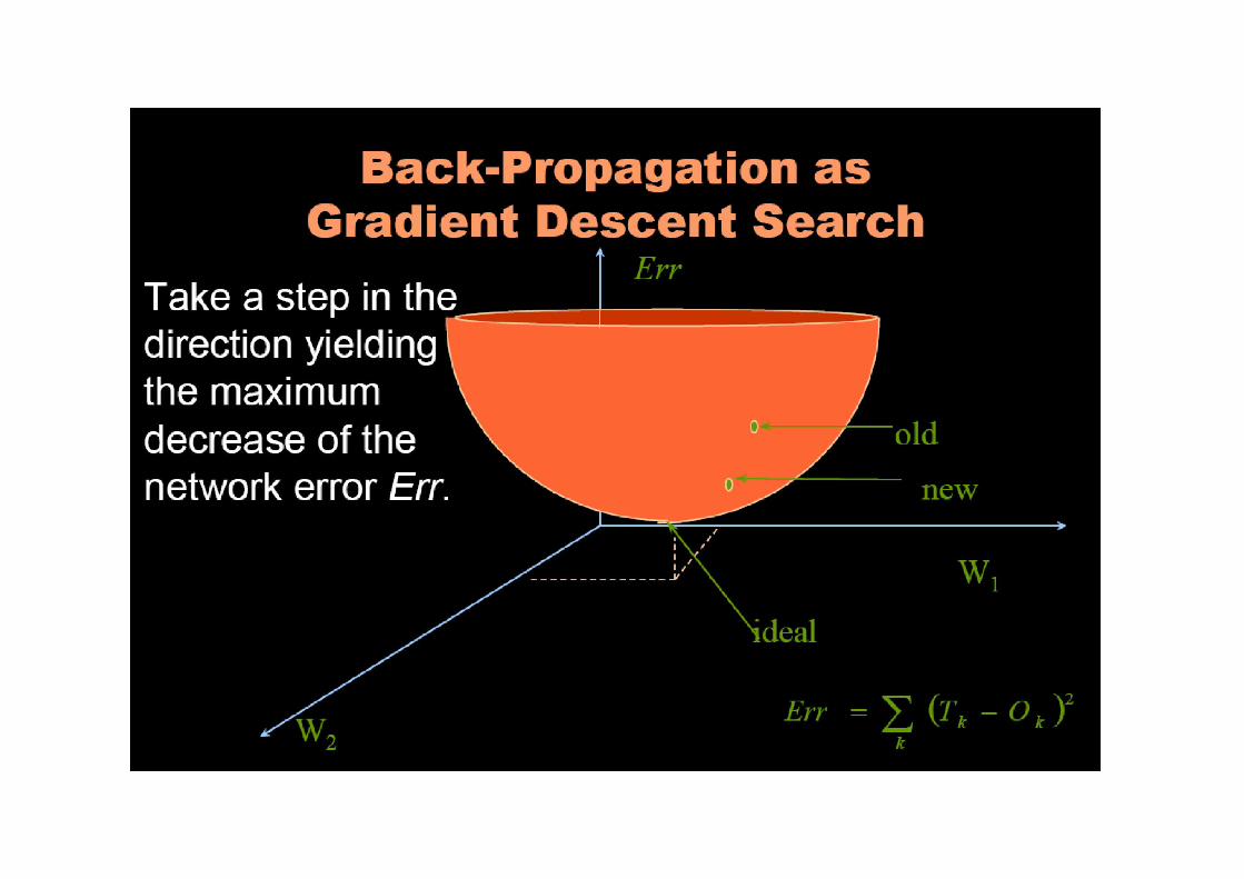
•This algorithm iteratively minimizes the network’s error by finding the gradient of the error surface in weight-space and adjusting the weights in the opposite direction (gradient-descent technique).

Learning in the BPN
•Gradient-descent example: Finding the absolute minimum of a one-dimensional error function f(x):
f(x)
slope: f’(x0)
xx0 x1 = x0 - f’(x0)
•Repeat this iteratively until for some xi, f’(xi) is sufficiently close to 0.
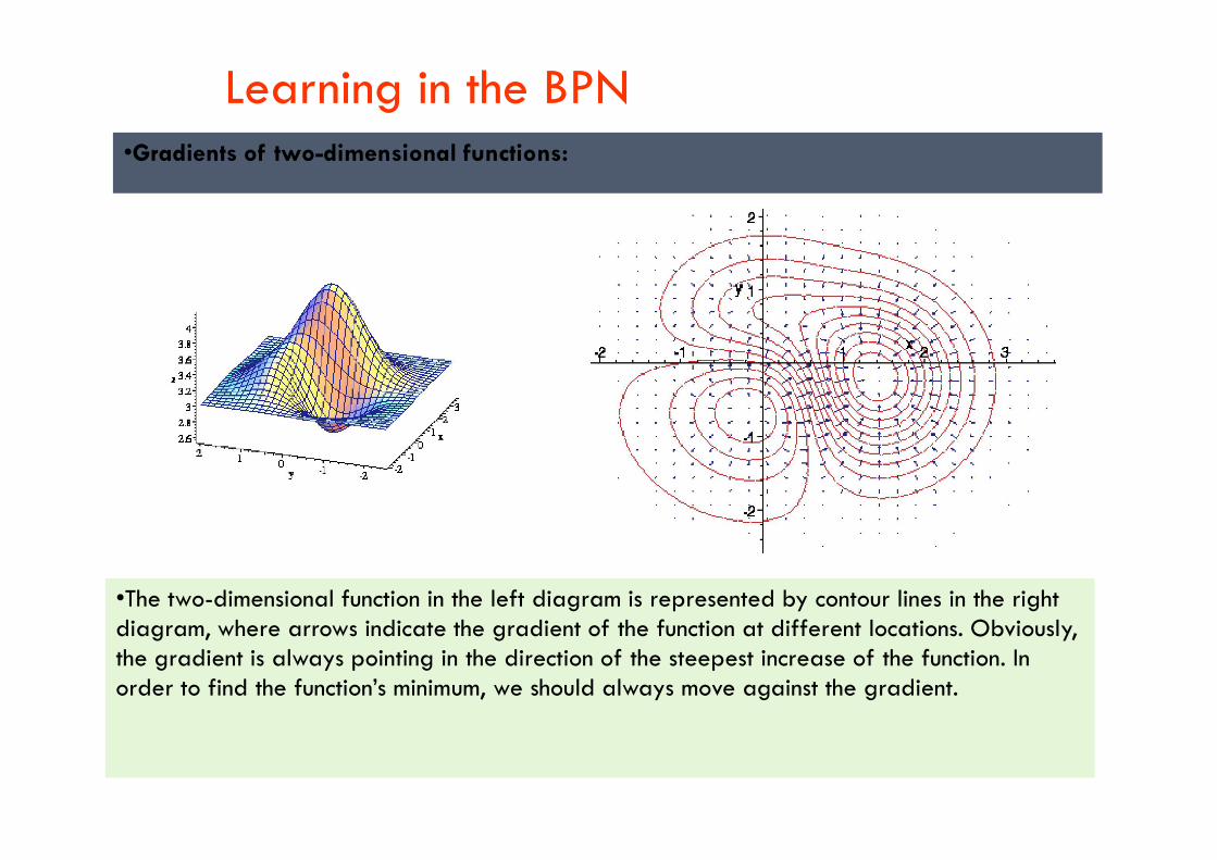
Learning in the BPN•Gradients of two-dimensional functions:
•The two-dimensional function in the left diagram is represented by contour lines in the right diagram, where arrows indicate the gradient of the function at different locations. Obviously, the gradient is always pointing in the direction of the steepest increase of the function. In order to find the function’s minimum, we should always move against the gradient.

Gradient Descent
(w1,w2)
(w1+w1,w2 +w2)(w1+w1,w2 +w2)
Learning in the BPN
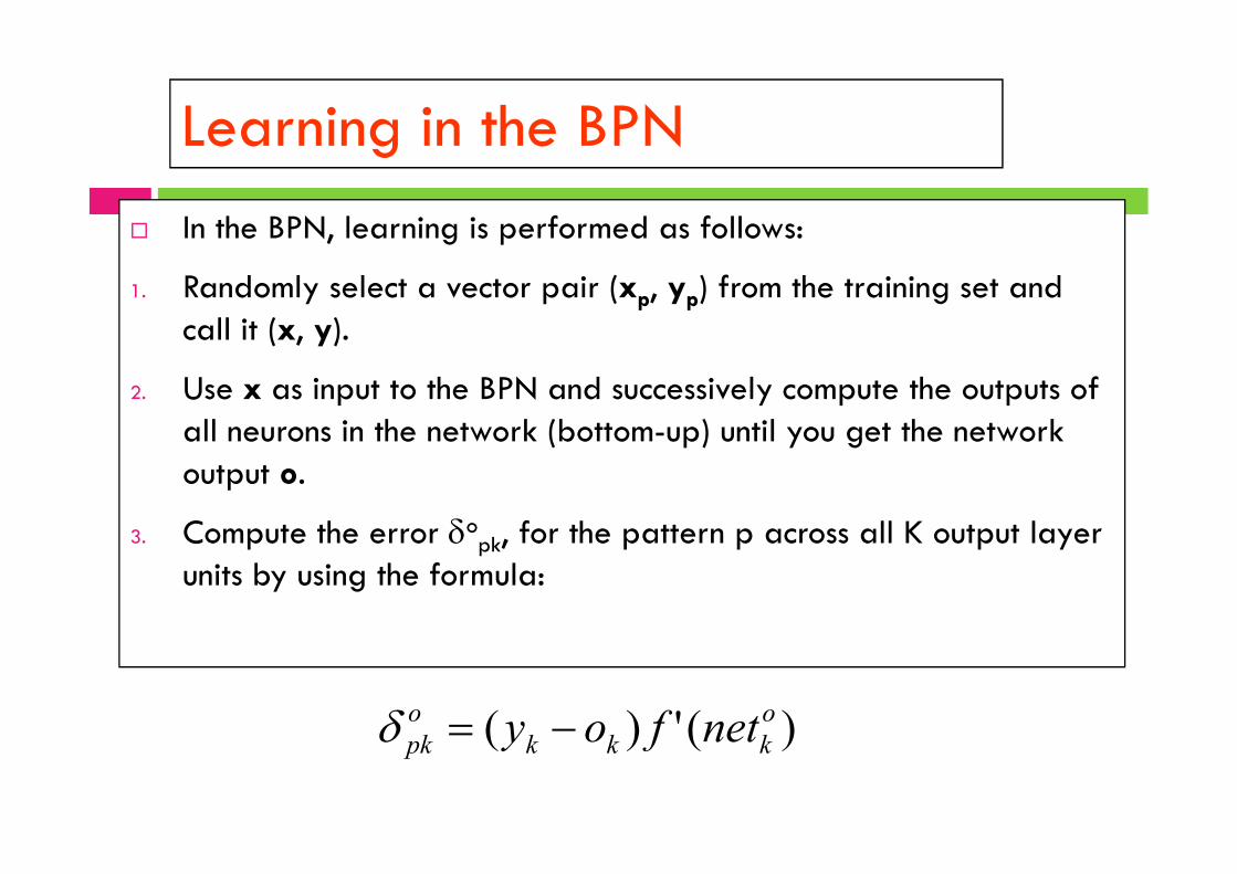
In the BPN, learning is performed as follows:
1. Randomly select a vector pair (xp, yp) from the training set and call it (x, y).
2. Use x as input to the BPN and successively compute the outputs of all neurons in the network (bottom-up) until you get the network all neurons in the network (bottom-up) until you get the network output o.
3. Compute the error opk, for the pattern p across all K output layer
units by using the formula:
)(')( okkk
opk netfoy
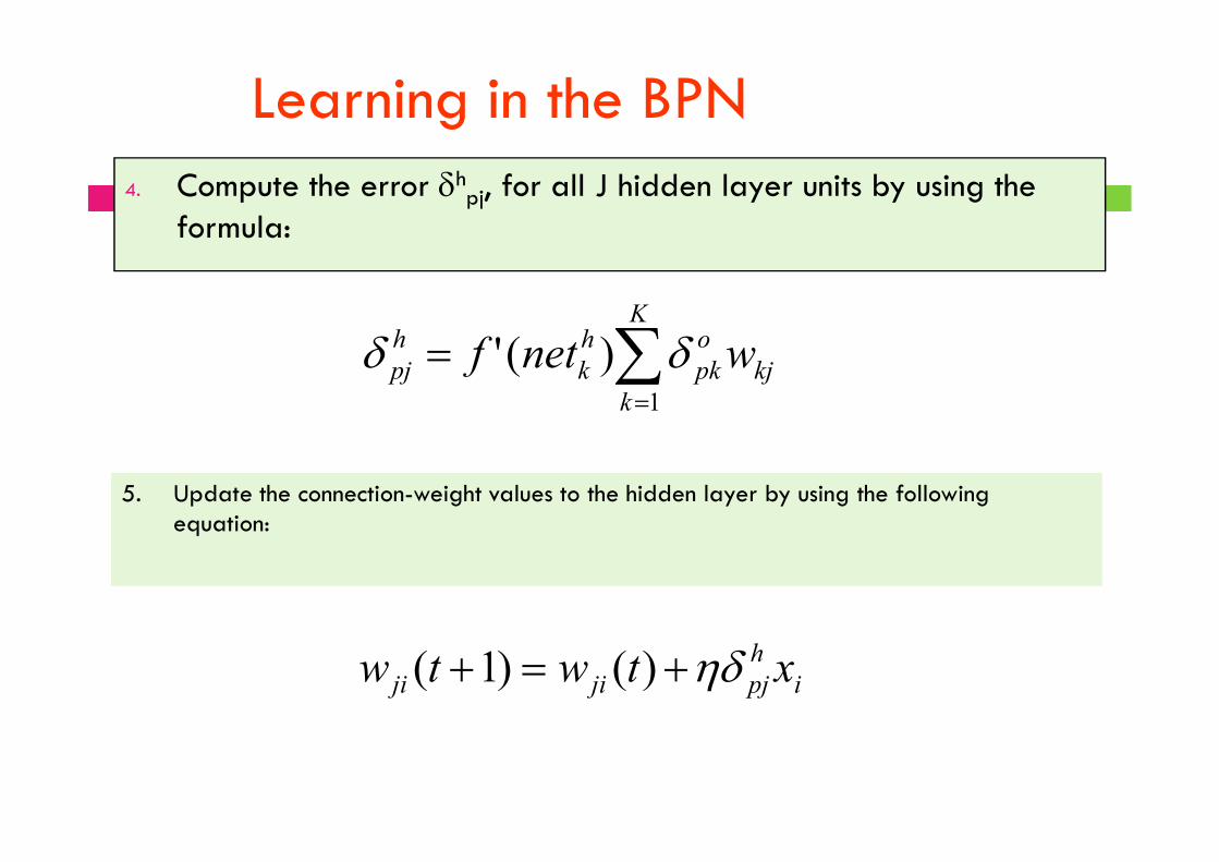
Learning in the BPN4. Compute the error h
pj, for all J hidden layer units by using the formula:
kj
K
k
opk
hk
hpj wnetf
1
)('
5. Update the connection-weight values to the hidden layer by using the following equation:
ihpjjiji xtwtw )()1(

Learning in the BPN
Repeat steps 1 to 6 for all vector pairs in the training set; this is
6. Update the connection-weight values to the output layer by using the following equation:
)()()1( hj
opkkjkj netftwtw
Repeat steps 1 to 6 for all vector pairs in the training set; this is called a training epoch.
Run as many epochs as required to reduce the network error E to fall below a threshold :
2
1 1
)(
P
p
K
k
opkE
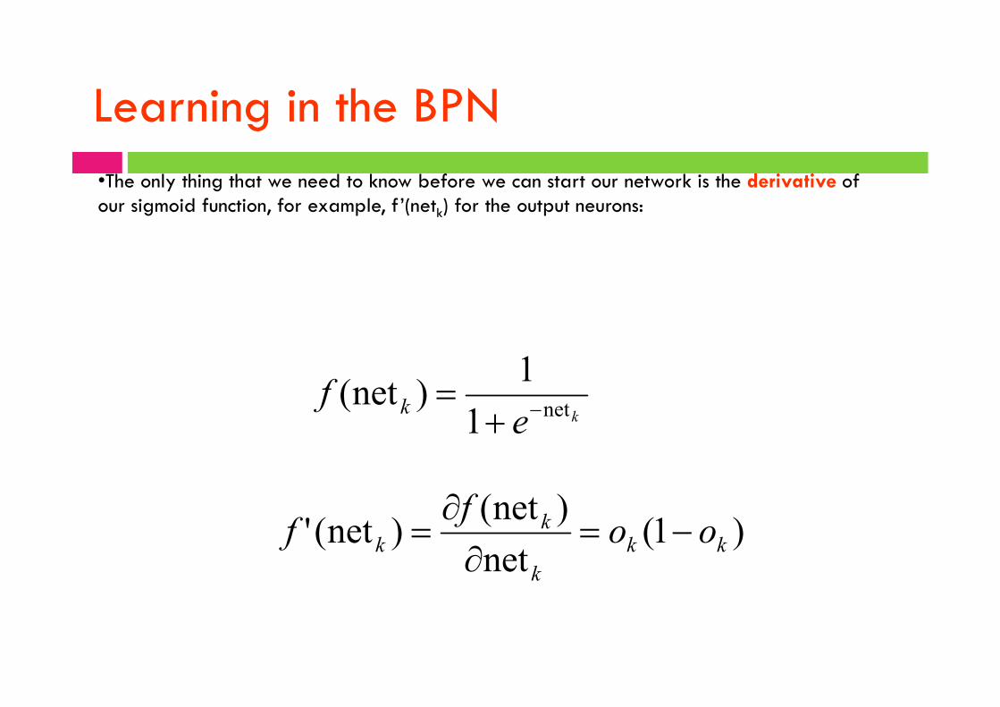
Learning in the BPN
•The only thing that we need to know before we can start our network is the derivative of our sigmoid function, for example, f’(netk) for the output neurons:
1ke
f k net1
1)net(
)1(net
)net()net(' kk
k
kk oo
ff
Learning in the BPN
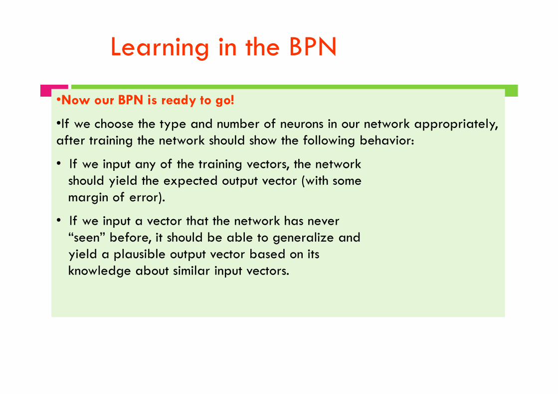
•Now our BPN is ready to go!
•If we choose the type and number of neurons in our network appropriately, after training the network should show the following behavior:
• If we input any of the training vectors, the network should yield the expected output vector (with some margin of error).margin of error).
• If we input a vector that the network has never “seen” before, it should be able to generalize and yield a plausible output vector based on its knowledge about similar input vectors.
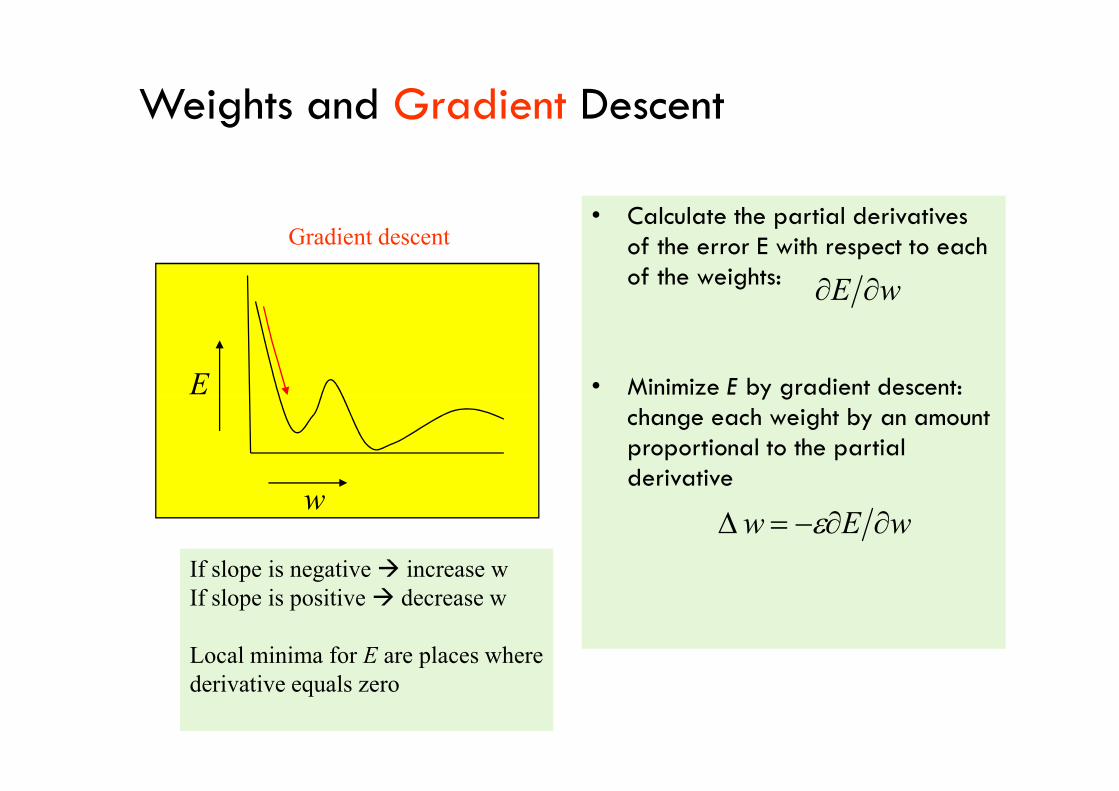
Weights and Gradient Descent
• Calculate the partial derivatives of the error E with respect to each of the weights:
• Minimize E by gradient descent:
wE
E
Gradient descent
• Minimize E by gradient descent: change each weight by an amount proportional to the partial derivative
E
w
If slope is negative increase wIf slope is positive decrease w
Local minima for E are places wherederivative equals zero
wEw

Gradient descent
Error
Local minimum
Global minimum

Faster Convergence: Momentum rule
• Add a fraction (a=momentum) of the last change to the current change
)1()( twwEtw a
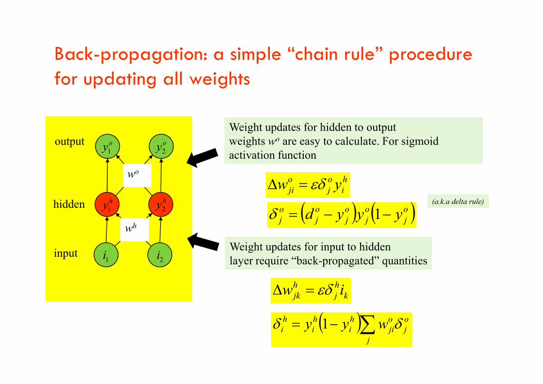
Back-propagation: a simple “chain rule” procedure for updating all weights
outputWeight updates for hidden to output weights wo are easy to calculate. For sigmoid activation function
hi
oj
oji yw
wo
oy1oy2
input
hidden
ijji yw
wh
Weight updates for input to hidden layer require “back-propagated” quantities
oj
oj
oj
oj
oj yyyd 1
hy1
hy2
1i 2i
j
oj
oji
hi
hi
hi wyy 1
khj
hjk iw
(a.k.a delta rule)
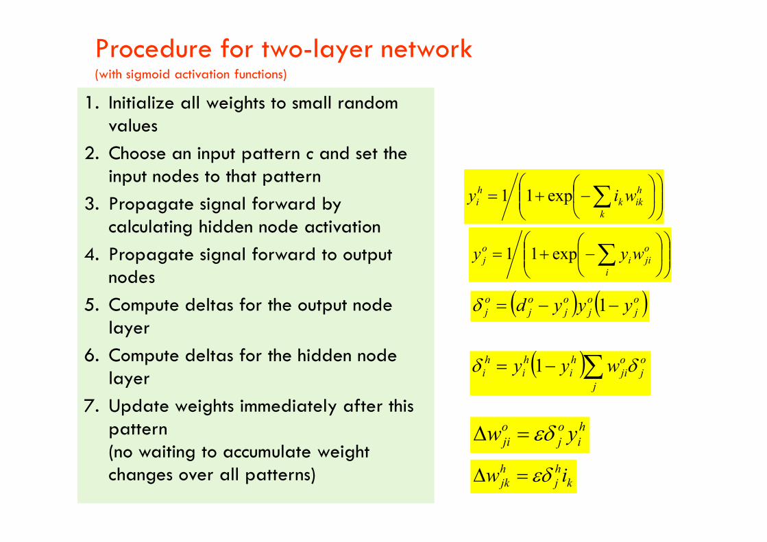
Procedure for two-layer network (with sigmoid activation functions)
1. Initialize all weights to small random values
2. Choose an input pattern c and set the input nodes to that pattern
3. Propagate signal forward by calculating hidden node activation
4. Propagate signal forward to output nodes
k
hikk
hi wiy exp11
i
ojii
oj wyy exp11
nodes
5. Compute deltas for the output node layer
6. Compute deltas for the hidden node layer
7. Update weights immediately after this pattern (no waiting to accumulate weight changes over all patterns)
i
oj
oj
oj
oj
oj yyyd 1
j
oj
oji
hi
hi
hi wyy 1
hi
oj
oji yw
khj
hjk iw

Artificial Neural Networks
Perceptrons
o(x1,x2...,xn) = 1 if w0+ w1 x1+.. + wn xn > 00
-1 otherwise
o(x) = sgn(w.x) (x0=1)
Hypothesis Space: H = {w | w n+1}


Artificial Neural Networks
• Representational Power
– Perceptrons can represent all the primitive Boolean functions AND, OR, NAND (AND) and Boolean functions AND, OR, NAND (AND) and NOR (OR)
– They cannot represent all Boolean functions (for example, XOR)
– Every Boolean function can be represented by some network of perceptrons two levels deep

Artificial Neural Networks
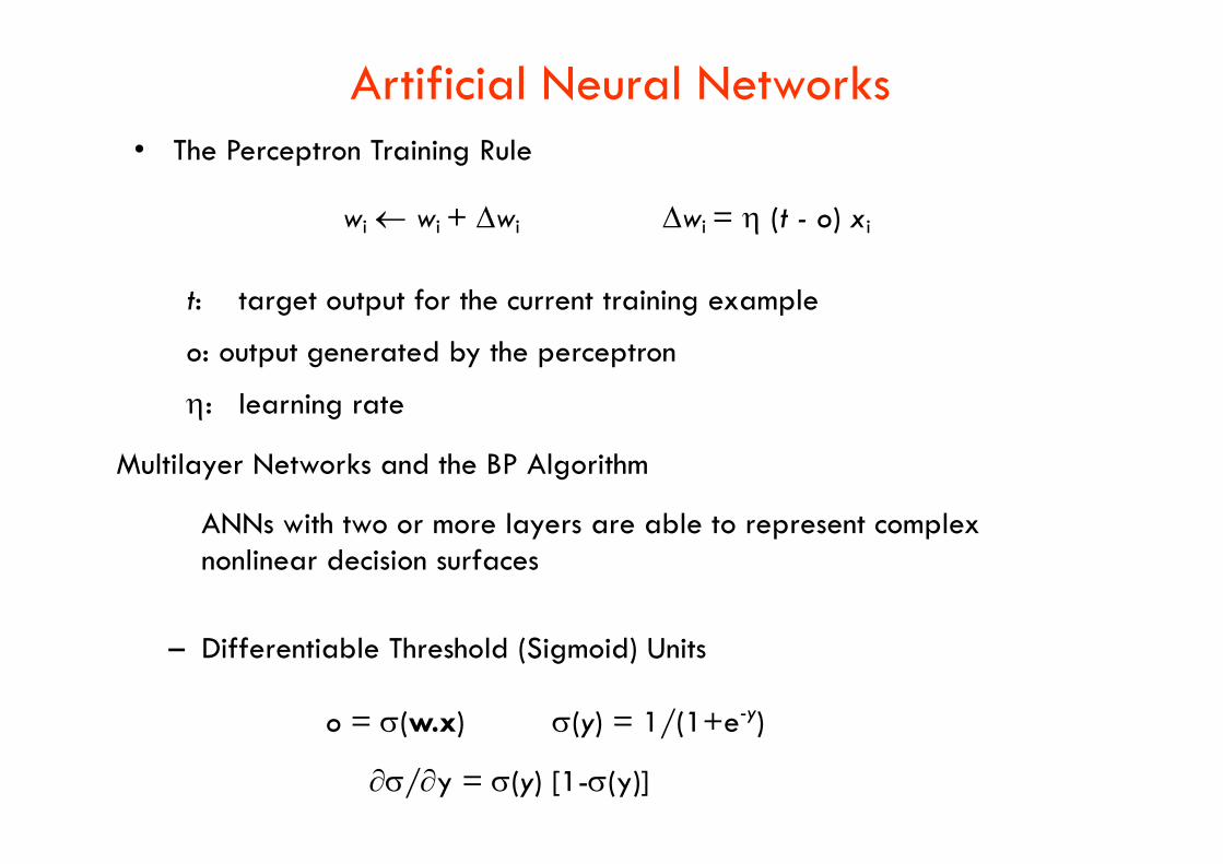
• The Perceptron Training Rule
wi wi + wi wi = (t - o) xi
t: target output for the current training example
o: output generated by the perceptron
: learning rate
Artificial Neural Networks
Multilayer Networks and the BP Algorithm
ANNs with two or more layers are able to represent complex nonlinear decision surfaces
– Differentiable Threshold (Sigmoid) Units
o = (w.x) (y) = 1/(1+e-y)
/y = (y) [1-(y)]

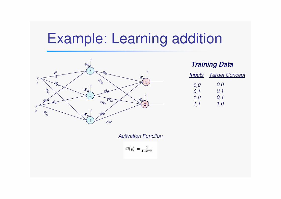

Example: Learning addition
First find the outputs OI , OII . In order to do this, propagate the inputs forward. First find the outputs for the neurons of hidden layer
)1.()(
)1.()(
)1.()(
2321310
3033
2221210
2022
2121110
1011
XWXWWOXWOO
XWXWWOXWOO
XWXWWOXWOO
iii
iii
iii

Example: Learning addition
)1.()(
)1.()(
3322110
0
3322110
0
OWOWOWWOOWOO
OWOWOWWOOWOO
IIIIIIi
IIiIIiII
IIIi
IiIiI
Then find the outputs of the neurons of output layer
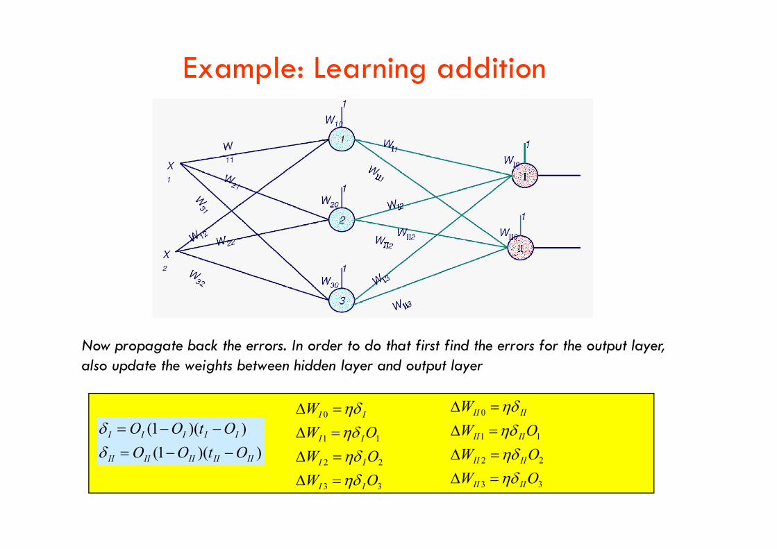
Example: Learning addition
Now propagate back the errors. In order to do that first find the errors for the output layer, also update the weights between hidden layer and output layer
))(1(
))(1(
IIIIIIIIII
IIIII
OtOO
OtOO
33
22
11
0
OW
OW
OW
W
II
II
II
II
33
22
11
0
OW
OW
OW
W
IIII
IIII
IIII
IIII

Example: Learning addition
And backpropagate the errors to hidden layer.
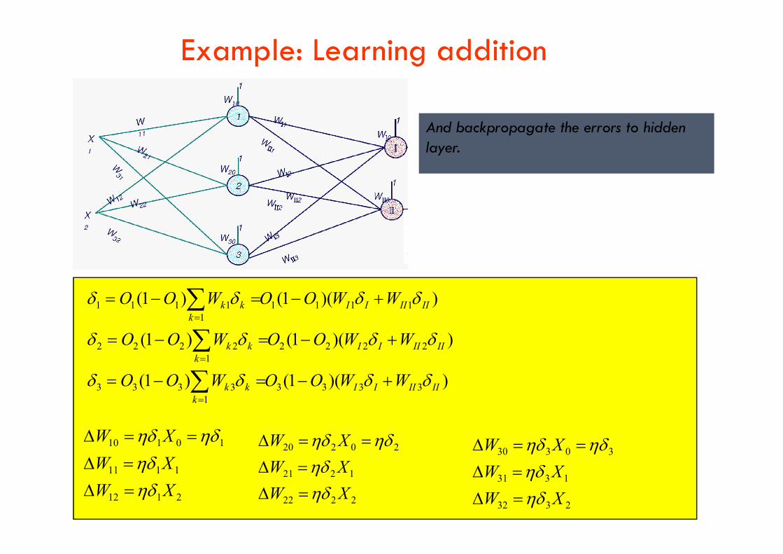
Example: Learning addition
And backpropagate the errors to hidden layer.
))(1()1(
))(1()1(
))(1()1(
33331
3333
22221
2222
11111
1111
IIIIIIk
kk
IIIIIIk
kk
IIIIIIk
kk
WWOOWOO
WWOOWOO
WWOOWOO
2112
1111
10110
XW
XW
XW
2222
1221
20220
XW
XW
XW
2332
1331
30330
XW
XW
XW

313131
303030
222222
212121
202020
121212
111111
101010
WWW
WWW
WWW
WWW
WWW
WWW
WWW
WWW
WWW
Example: Learning addition
333
222
111
000
333
222
111
000
323232
IIIIII
IIIIII
IIIIII
IIIIII
III
III
III
III
WWW
WWW
WWW
WWW
WWW
WWW
WWW
WWW
WWW
Finally update weights!!!!


Gradient-Descent Training Rule
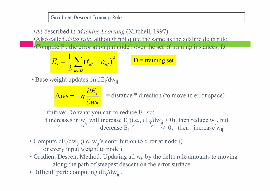
•As described in Machine Learning (Mitchell, 1997).•Also called delta rule, although not quite the same as the adaline delta rule. •Compute Ei, the error at output node i over the set of training instances, D.
iij
Ew
• Base weight updates on dEi/dwij
2)(
2
1
Dd
ididi otE D = training set
= distance * direction (to move in error space)ij
iij
ww
Intuitive: Do what you can to reduce Ei, so: If increases in wij will increase Ei (i.e., dEi/dwij > 0), then reduce wij, but
” ” decrease Ei ” ” < 0, then increase wij
• Compute dEi/dwij (i.e. wij’s contribution to error at node i) for every input weight to node i.
• Gradient Descent Method: Updating all wij by the delta rule amounts to movingalong the path of steepest descent on the error surface.
• Difficult part: computing dEi/dwij .
= distance * direction (to move in error space)
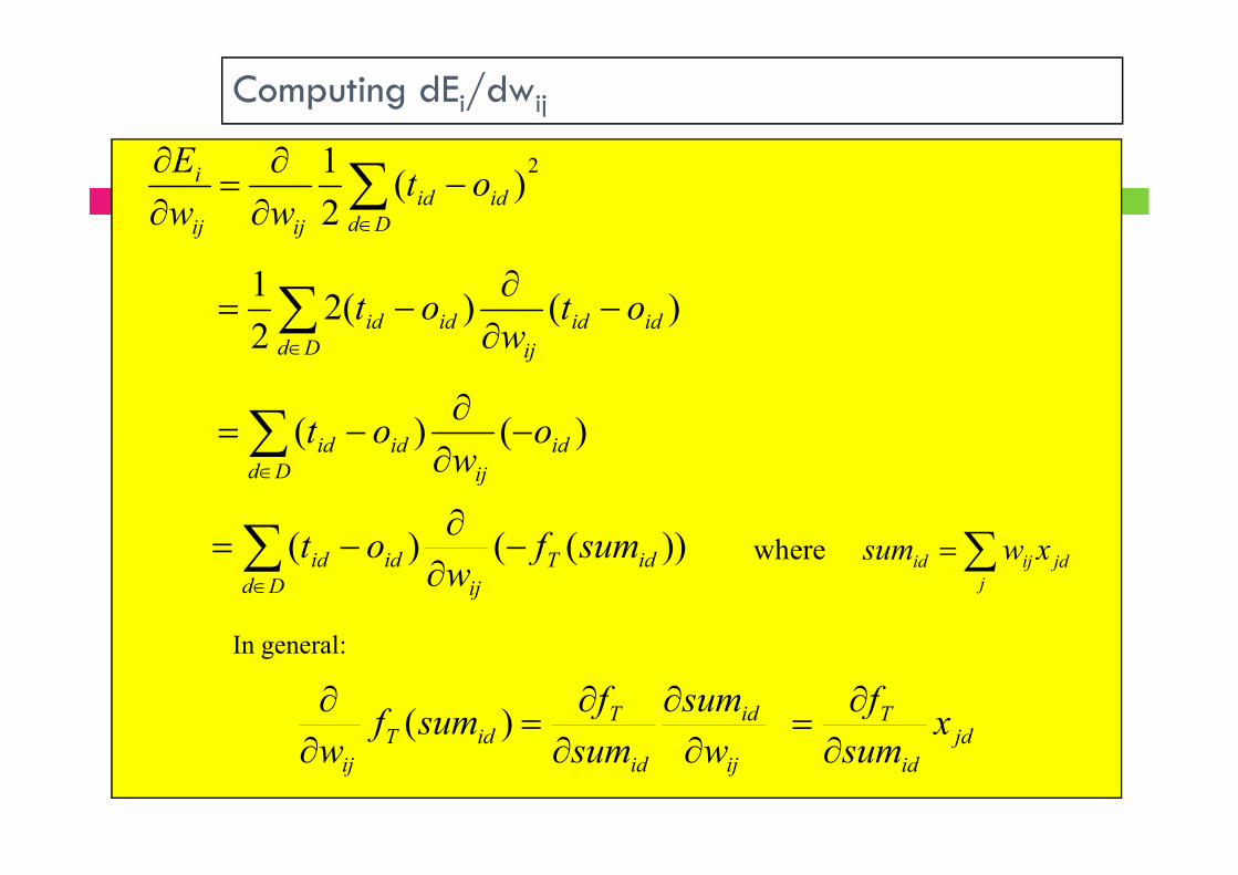
Computing dEi/dwij
2)(
2
1
Ddidid
ijij
i otww
E
)()(22
1idid
ijDdidid ot
wot
)()( ididid oot
)()( id
ijDdidid o
wot
))(()( idT
ijDdidid sumf
wot
jjdijid xwsumwhere
ij
id
id
TidT
ij w
sum
sum
fsumf
w
)( jd
id
T xsum
f
In general:

Computing )( idT
ij
sumfw
ididT sumsumf )(Identity ft :
1
id
id
T
id
sumsum
fsum
jdjd
ij
id
id
TidT
ij
xxw
sum
sum
fsumf
w
)1()(
idsumidTe
sumf
1
1)(Sigmoidal ft :
))(1)(()1(1
12 idtidtsum
sum
sumid
sumfsumfe
e
esum id
id
id
ididT osumf )(But since: jdidididT
ij
xoosumfw
)1()(
If fT is not continuous, andhence not differentiableeverywhere, then we cannotuse the Delta Rule.

Weight Updates for Simple Units
)()( xot
))(()( idT
ijDdidid
ij
i sumfw
otw
E
fT = identity function
)()( jdDd
idid xot
jdDd
idid
ij
iij xot
w
Ew
)(
wij
xjd
oid
tid
Eid
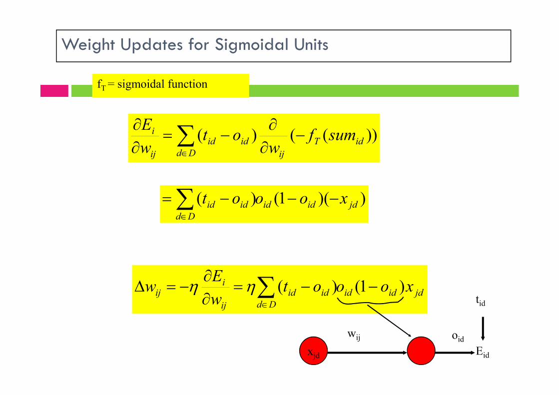
Weight Updates for Sigmoidal Units
))(1()( xooot
))(()( idT
ijDdidid
ij
i sumfw
otw
E
fT = sigmoidal function
))(1()( jdididDd
idid xooot
jdididDd
idid
ij
iij xooot
w
Ew )1()(
wij
xjd
oid
tid
Eid

Error gradient for the sigmoid function
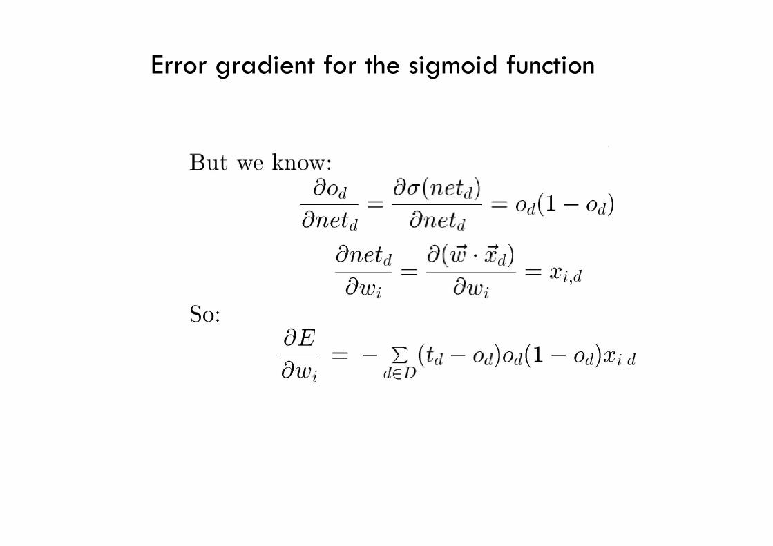
Error gradient for the sigmoid function
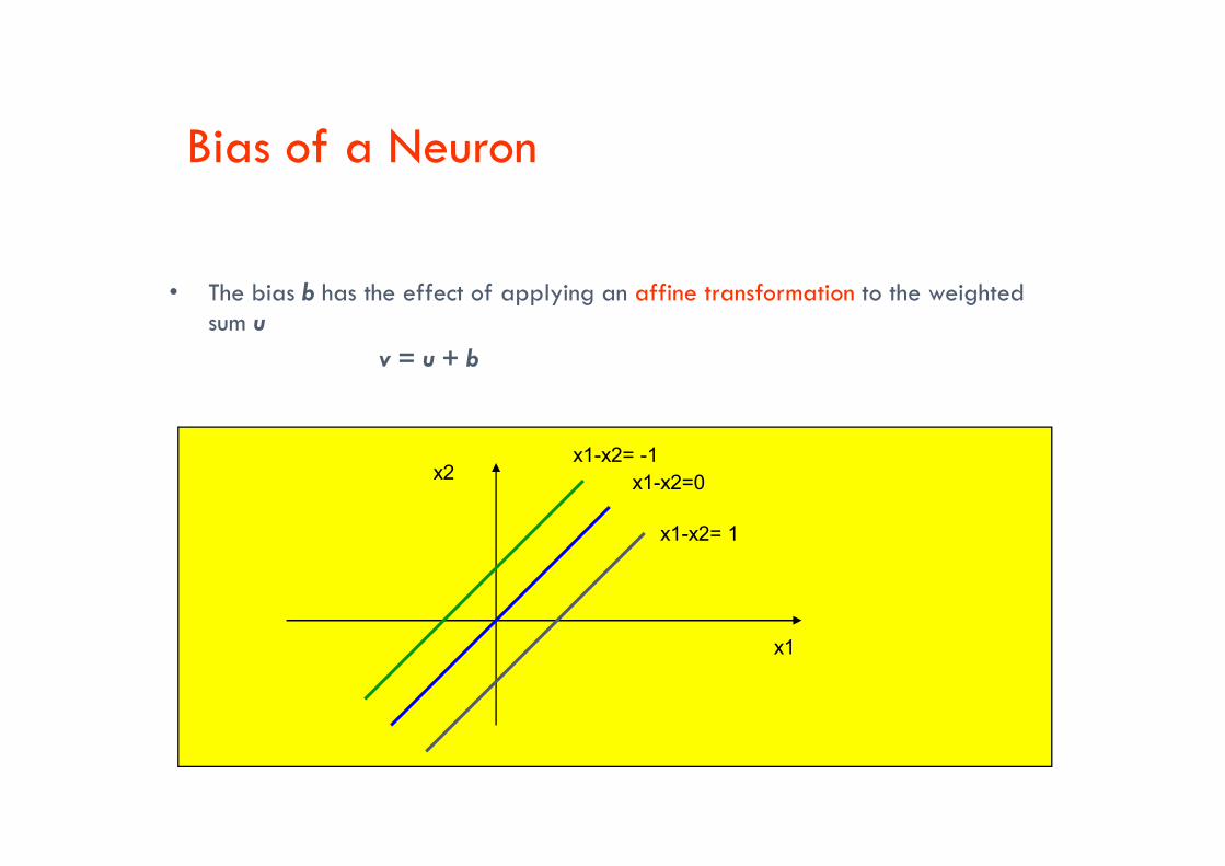
Bias of a Neuron
• The bias b has the effect of applying an affine transformation to the weighted sum u
v = u + b
x1-x2=0
x1-x2= 1
x1
x2x1-x2= -1

Bias as extra input•• The bias is an external parameter of the neuron. It can be modeled by adding an extra input.
Activationx1 w1
w0x0 = +1
bw
xwv j
m
j
j
0
0
Inputsignal
Synapticweights
Summingfunction
ActivationfunctionLocal
Fieldv
Outputyx2
xm
w2
wm
w1
)(
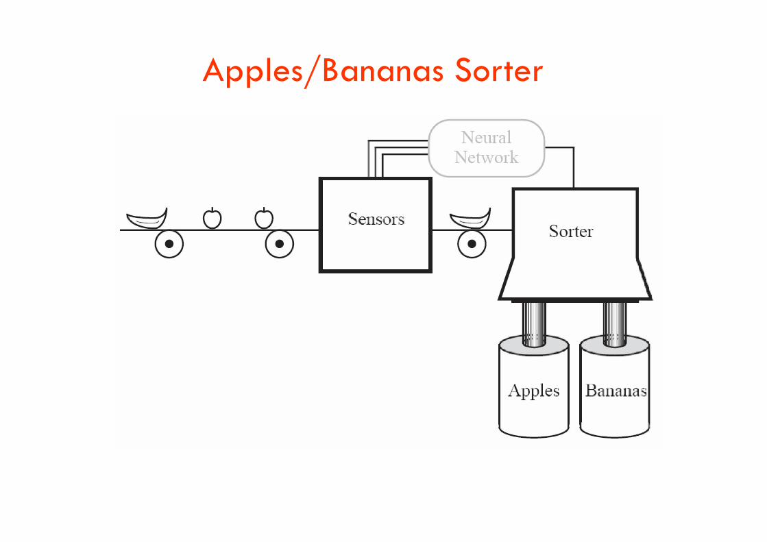
Apples/Bananas Sorter


Prototype Vectors

Perceptron

Two-Input Case
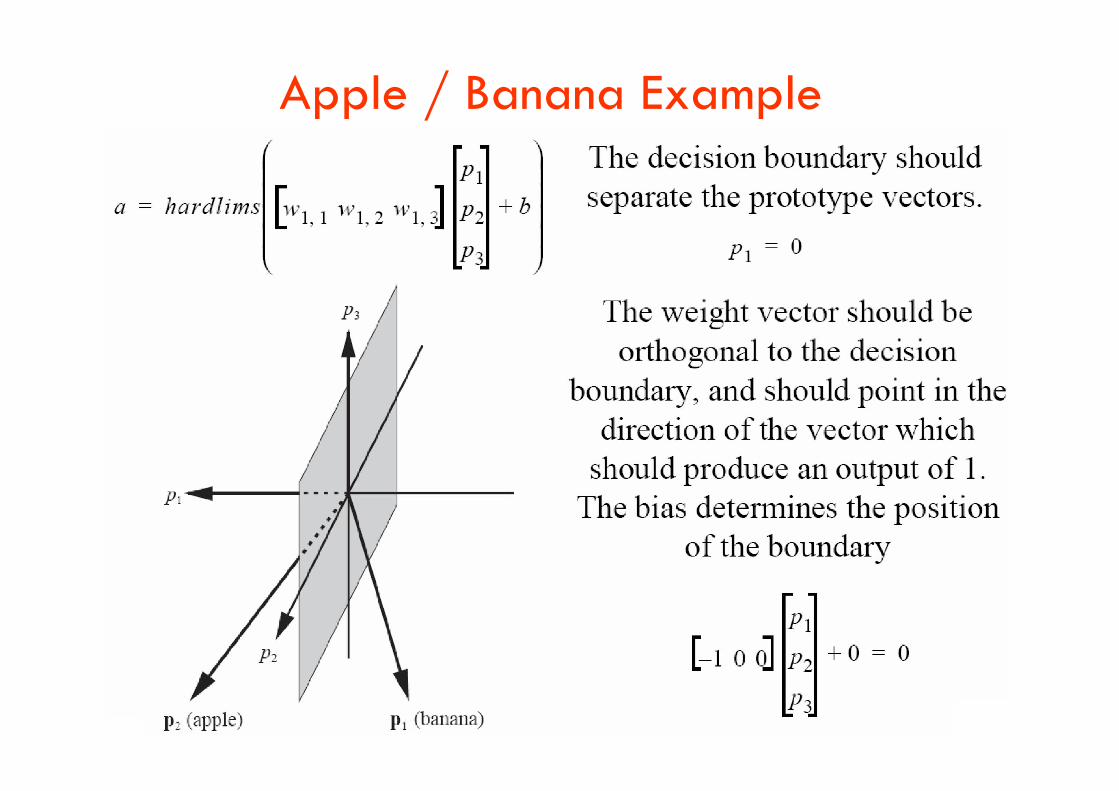
Apple / Banana Example

Testing the Network

References
An introduction to neural computing. Alexander, I. and Morton, H. 2nd edition
http://media.wiley.com/product_data/excerpt/19/04713491/0471349119.pdf
Neural Networks at Pacific Northwest National Laboratoryhttp://www.emsl.pnl.gov:2080/docs/cie/neural/neural.homepage.html
Industrial Applications of Neural Networks (research reports Esprit, I.F.Croall, J.P.Mason)
A Novel Approach to Modeling and Diagnosing the Cardiovascular Systemhttp://www.emsl.pnl.gov:2080/docs/cie/neural/papers2/keller.wcnn95.abs.html
Artificial Neural Networks in Medicine Artificial Neural Networks in Medicinehttp://www.emsl.pnl.gov:2080/docs/cie/techbrief/NN.techbrief.html
Neural Networks by Eric Davalo and Patrick Naim
Learning internal representations by error propagation by Rumelhart, Hinton and Williams (1986).
Klimasauskas, CC. (1989). The 1989 Neuron Computing Bibliography. Hammerstrom, D. (1986). A Connectionist/Neural Network Bibliography.
DARPA Neural Network Study (October, 1987-February, 1989). MIT Lincoln Lab. Neural Networks, Eric Davalo and Patrick Naim
Assimov, I (1984, 1950), Robot, Ballatine, New York.
Electronic Noses for Telemedicinehttp://www.emsl.pnl.gov:2080/docs/cie/neural/papers2/keller.ccc95.abs.html
Pattern Recognition of Pathology Imageshttp://kopernik-eth.npac.syr.edu:1200/Task4/pattern.html


