1 PHYS 352 Signal Conditioning: Analog Filters Analog Filters reasons to use analog filters restrict bandwidth, improving signal-to-noise accomplish some impedance matching along with amplifiers integration and differentiation note: this course is systems-level not so concerned about noise characteristics of individual transistors, for example we want to examine general ways to condition signals in measurement systems so, coming up, a qualitative overview look at analog filters
Transcript
1
PHYS 352
Signal Conditioning: Analog Filters
Analog Filters reasons to use analog filters
restrict bandwidth, improving signal-to-noise accomplish some impedance matching
along with amplifiers
integration and differentiation
note: this course is systems-level not so concerned about noise characteristics of
individual transistors, for example we want to examine general ways to condition
signals in measurement systems so, coming up, a qualitative overview look at
analog filters
2
Filters: General Issues average out noise eliminate high frequencies but, in general
1/f noise may also be present signal may have high frequency content
you don’t want to filter out
in general, need to consider bandpass
Want a Fast Roll-off e.g. RC low-pass filter what’s important is the
order of the polynomial in the denominator determines how fast the
function drops off 20*n dB/decade, where n
is the number of “poles”
cascade one low-pass filter after another (identical or different RC) for faster roll-off?
one pole, n=1
two poles, n=2
3
Passive Analog Filters simply cascading RC low-pass filters
does not work well because though it does produce steeper
falloff, going as 20*n dB/decade, where n is the number of RC stages
each successive stage loads the previous filter response not just based
upon ω = 1/RC in each stage the “knee” remains soft
bandwidth what cutoff frequency?
roll-off: how fast? sharp transition stopband attenuation
how deep? passband/stopband ripple
how flat? phase shift
what happens to output pulse shape if the phase response is not constant with frequency?
input output
desire output signal to resemble input; even if two signals at ω1 and ω2 are passed with A(ω1)=A(ω2), the output looks different if they have different phase shift
Key Filter Design Criteria
4
rise time overshoot ringing settling time
keep these in mind also; however, we'll focus on frequency domain analysis of performance
both amplitude and phase response impact time-domain performance
Filter Performance in Time Domain
rise time
Bandpass Filters RC circuits
they can work; far from ideal though
passive RLC filters can achieve virtually any desired flatness
of the passband combined with sharpness of transition and steepness of falloff
however, inductors are bulky, “expensive”, not lossless (finite resistance), prone to magnetic pickup of interference, winding-induced non-linearity
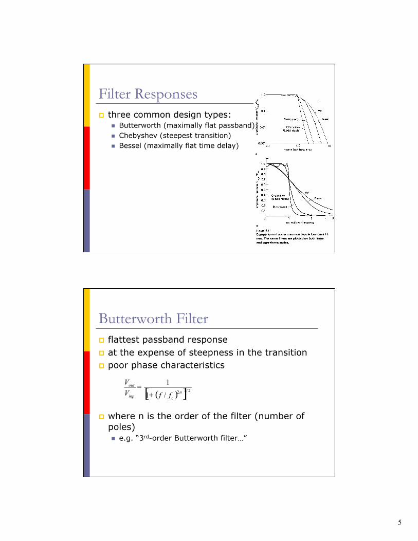
flattest passband response at the expense of steepness in the transition poor phase characteristics
where n is the order of the filter (number of poles) e.g. “3rd-order Butterworth filter…”
Butterworth Filter
6
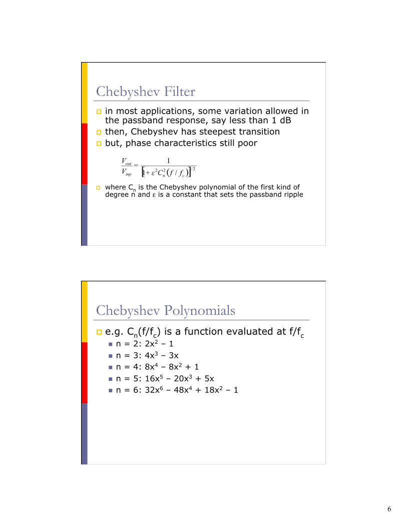
in most applications, some variation allowed in the passband response, say less than 1 dB
then, Chebyshev has steepest transition but, phase characteristics still poor
where Cn is the Chebyshev polynomial of the first kind of degree n and ε is a constant that sets the passband ripple
Chebyshev Filter
Chebyshev Polynomials e.g. Cn(f/fc) is a function evaluated at f/fc
n = 2: 2x2 – 1 n = 3: 4x3 – 3x n = 4: 8x4 – 8x2 + 1 n = 5: 16x5 – 20x3 + 5x n = 6: 32x6 – 48x4 + 18x2 – 1
7
Butterworth versus Chebyshev Butterworth flat passband looks good, but is
already rolling off near the cutoff frequency, unlike Chebyshev
Chebyshev amplitude response variations are spread throughout passband
RLC components of finite tolerance will cause filter to deviate from the predicted response real-life Butterworth filter has some passband
ripple anyway
Bessel Filter is a linear-phase filter amplitude response is less steep than
Butterworth time-domain properties are (naturally)
better than Butterworth or Chebyshev it takes a higher order Bessel filter to
give the same steepness of the frequency response; but, linear phase (pulse-shape fidelity) may be worth it
8
Bessel Filter Transfer Function
where θn(s) is a reverse Bessel polynomial function, for example: n=1; s+1 n=2; s2+3s+3 n=3; s3+6s2+15s+15
so, again for example, a 3rd order Bessel low-pass transfer function is (in frequency units of ω0):
Example: 3rd Order Bessel Filter
9
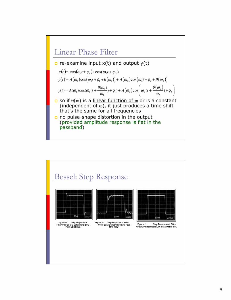
Linear-Phase Filter re-examine input x(t) and output y(t)
so if θ(ω) is a linear function of ω or is a constant (independent of ω), it just produces a time shift that’s the same for all frequencies
no pulse-shape distortion in the output (provided amplitude response is flat in the passband)
y t( )= A ω1( )cos ω1t +φ1+θ ω1( )( ) + A ω2( )cos ω2t +φ2 +θ ω2( )( )y(t) = A(ω1)cos(ω1(t +
θ(ω1)ω1
) + φ1) + A ω2( )cos ω2 (t +θ ω2( )ω2
)+φ2⎛⎝⎜
⎞⎠⎟
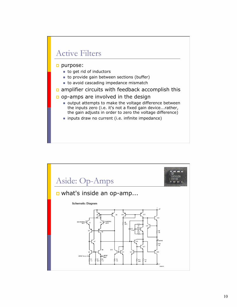
Bessel: Step Response
10
Active Filters purpose:
to get rid of inductors to provide gain between sections (buffer) to avoid cascading impedance mismatch
amplifier circuits with feedback accomplish this op-amps are involved in the design
output attempts to make the voltage difference between the inputs zero (i.e. it's not a fixed gain device...rather, the gain adjusts in order to zero the voltage difference)
inputs draw no current (i.e. infinite impedance)
Aside: Op-Amps what's inside an op-amp...
11
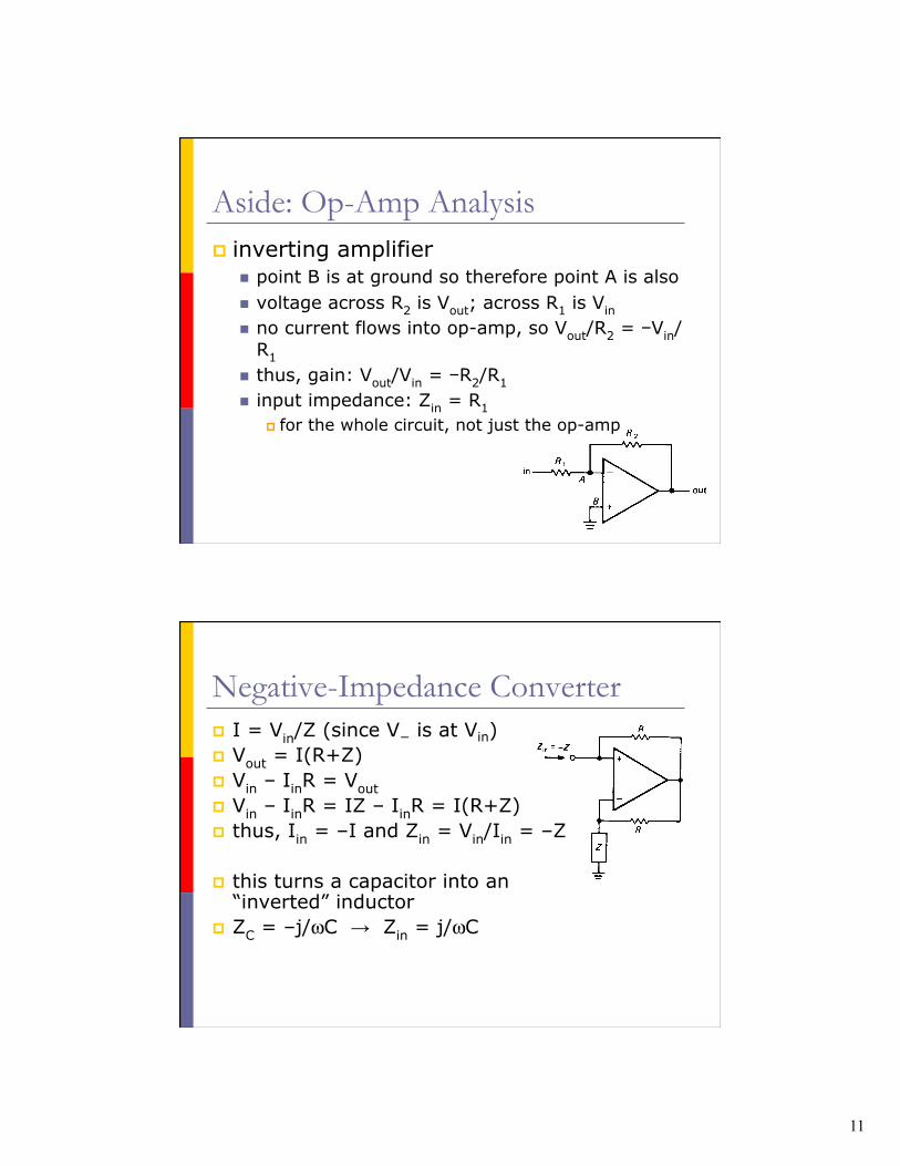
Aside: Op-Amp Analysis inverting amplifier
point B is at ground so therefore point A is also voltage across R2 is Vout; across R1 is Vin
no current flows into op-amp, so Vout/R2 = −Vin/R1
thus, gain: Vout/Vin = −R2/R1
input impedance: Zin = R1
for the whole circuit, not just the op-amp
I = Vin/Z (since V− is at Vin) Vout = I(R+Z) Vin – IinR = Vout Vin – IinR = IZ – IinR = I(R+Z) thus, Iin = –I and Zin = Vin/Iin = –Z
this turns a capacitor into an “inverted” inductor
ZC = –j/ωC → Zin = j/ωC
Negative-Impedance Converter
12
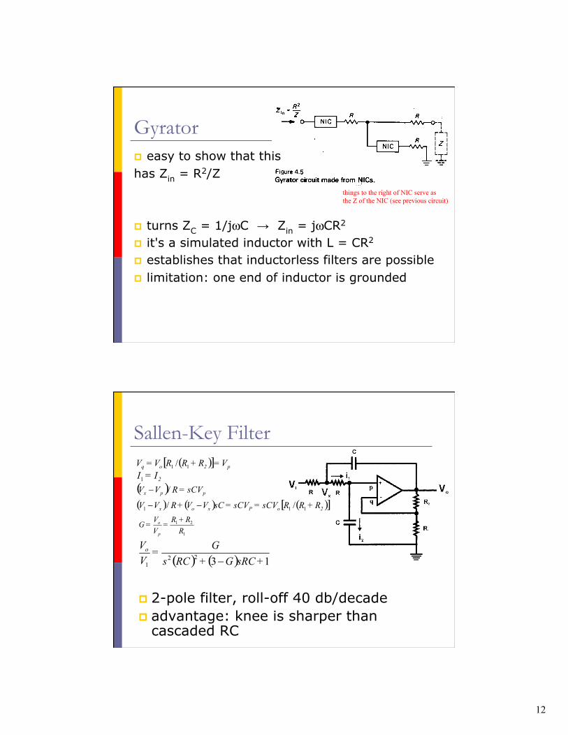
things to the right of NIC serve as the Z of the NIC (see previous circuit)
Gyrator easy to show that this has Zin = R2/Z
turns ZC = 1/jωC → Zin = jωCR2
it's a simulated inductor with L = CR2
establishes that inductorless filters are possible limitation: one end of inductor is grounded
2-pole filter, roll-off 40 db/decade advantage: knee is sharper than
cascaded RC
Sallen-Key Filter
13
VCVS Filter in general these are known as voltage-
controlled, voltage-source filters (VCVS filters); but, Sallen-Key filter is used interchangeably which itself is a generalization of the original Sallen-
Key filter which is strictly a unity gain filter
these are 2-pole filters cascade any number of 2-pole VCVS to
generate higher-order filters (individual filter sections not necessarily identical)
VCVS Filter Table suitable choice of components generates desired
response
14
VCVS Filter Table cont'd design table is for equal R, equal C
adjust the gain and RC = 1/2πfnfc for desired response
if multiple stages, each have different gain and fn
for high pass, interchange R and C, gain is the same, but inverted fn (“high” fn = 1/fn from “low” table)
for band pass, put a low-pass and high-pass together
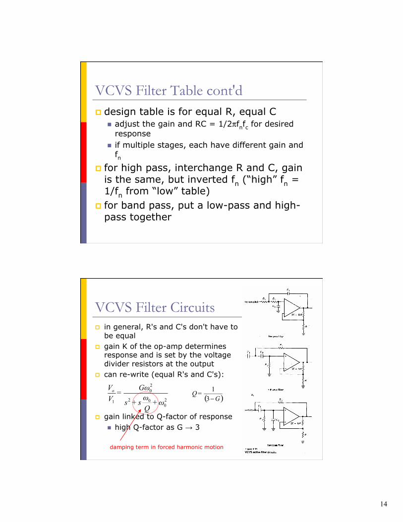
in general, R's and C's don't have to be equal
gain K of the op-amp determines response and is set by the voltage divider resistors at the output
can re-write (equal R's and C's):
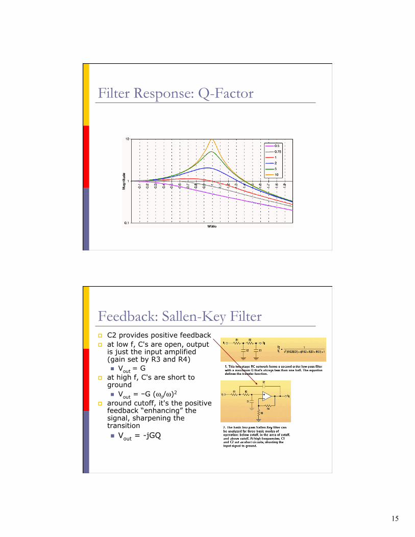
gain linked to Q-factor of response high Q-factor as G → 3
VCVS Filter Circuits
damping term in forced harmonic motion
15
Filter Response: Q-Factor
Feedback: Sallen-Key Filter C2 provides positive feedback at low f, C's are open, output
is just the input amplified (gain set by R3 and R4) Vout = G
at high f, C's are short to ground Vout = −G (ω0/ω)2
around cutoff, it's the positive feedback “enhancing” the signal, sharpening the transition Vout = -jGQ
16
Sallen-Key Limitation gain must be less than 3 otherwise, the circuit becomes unstable
resultant high Q with gain = 3 exhibits large sensitivity to variations in R3 and R4 imagine Q = 10, G = 2.9; if the “gain” resistors
change by 1%, the new Q = 16...unstable imagine Q = 1, G = 2; if “gain” resistors change by
1%, the new Q = 1.02...much better behaved
higher gain (negative Q) leads to oscillations
Concluding Remarks: Active Filters
there are books and books on active filters
many ways to achieve desired response (Bessel, Chebyshev, etc.)
some designs attempt to compensate for non-ideal behaviour of the op-amp