42
1 Probability Theory in Digital Communication
| Date post: | 17-Jul-2016 |
| Category: |
Documents |
| Upload: | himaanshu09 |
| View: | 240 times |
| Download: | 0 times |

1
Probability Theory in Digital Communication

2
An Example: Binary Symmetric Channel
Consider a discrete memoryless channel to transmit binary data
Assume the channel as symmetric, which means
the probability of receiving symbol 1 when symbol 0 is sent is the same as the probability of receiving symbol 0 when symbol 1 is sent
To describe the probabilistic nature of this channel fully, we need two sets of probabilities
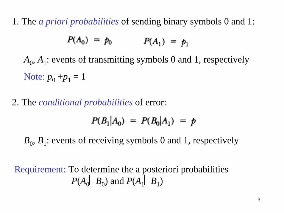
3
1. The a priori probabilities of sending binary symbols 0 and 1:
A0, A1: events of transmitting symbols 0 and 1, respectively
Note: p0 +p1 = 1
2. The conditional probabilities of error:
B0, B1: events of receiving symbols 0 and 1, respectively
Requirement: To determine the a posteriori probabilities P(A0⎮B0) and P(A1⎮B1)
4
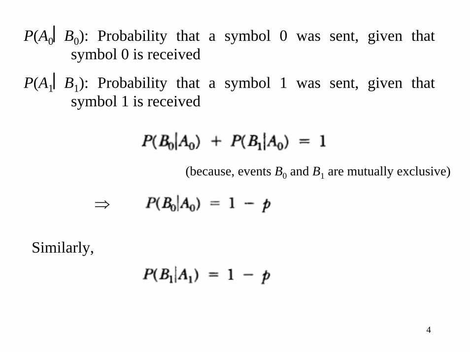
P(A0⎮B0): Probability that a symbol 0 was sent, given that symbol 0 is received
P(A1⎮B1): Probability that a symbol 1 was sent, given that symbol 1 is received
(because, events B0 and B1 are mutually exclusive)
⇒
Similarly,

5
[Transition probability diagram of BSC]
From the figure,
1. The probability of receiving symbol 0 is given by

6
2. The probability of receiving symbol 1 is given by
Application of Baye’s rule gives

7
Random Variables:
• The outcome of a random experiment
may be a real number (as in case of rolling a die) or it may be non-numerical and described by a
phrase (such as “heads” or “tails” in tossing a coin)
• From a mathematical point of view, it is desirable to have numerical values for all outcomes. For this reason, we assign a real number to each sample point according to some rule
Defn.: A function whose domain is a sample space and whose range is some set of real numbers is called a random variable of the experiment
Note: It is a function that maps sample points into real numbers
8
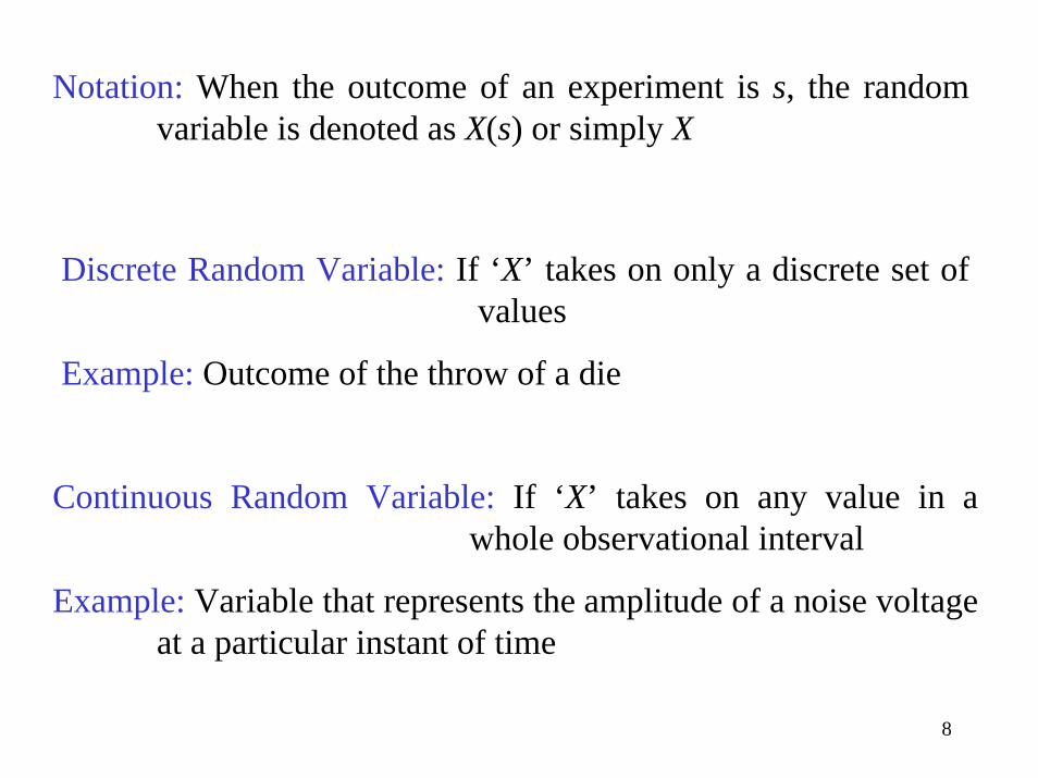
Notation: When the outcome of an experiment is s, the random variable is denoted as X(s) or simply X
Discrete Random Variable: If ‘X’ takes on only a discrete set of values
Example: Outcome of the throw of a die
Continuous Random Variable: If ‘X’ takes on any value in a whole observational interval
Example: Variable that represents the amplitude of a noise voltage at a particular instant of time

9
Cumulative Distribution Function:
The CDF FX(x) of a random variable X is the probability that Xtakes a value less than or equal to x; i.e.,
Note: For any point x, the distribution function FX(x) expresses a probability
A CDF FX(x) has the following properties:
1. FX(x) ≥ 0 2. FX(∞) = 1 3. FX(-∞) = 0
4. FX(x) is a monotone non-decreasing function of x; i.e.,
FX(x1) ≤ FX(x2) if x1 ≤ x2
10
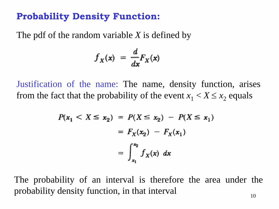
Probability Density Function:
The pdf of the random variable X is defined by
Justification of the name: The name, density function, arises from the fact that the probability of the event x1 < X ≤ x2 equals
The probability of an interval is therefore the area under the probability density function, in that interval
11
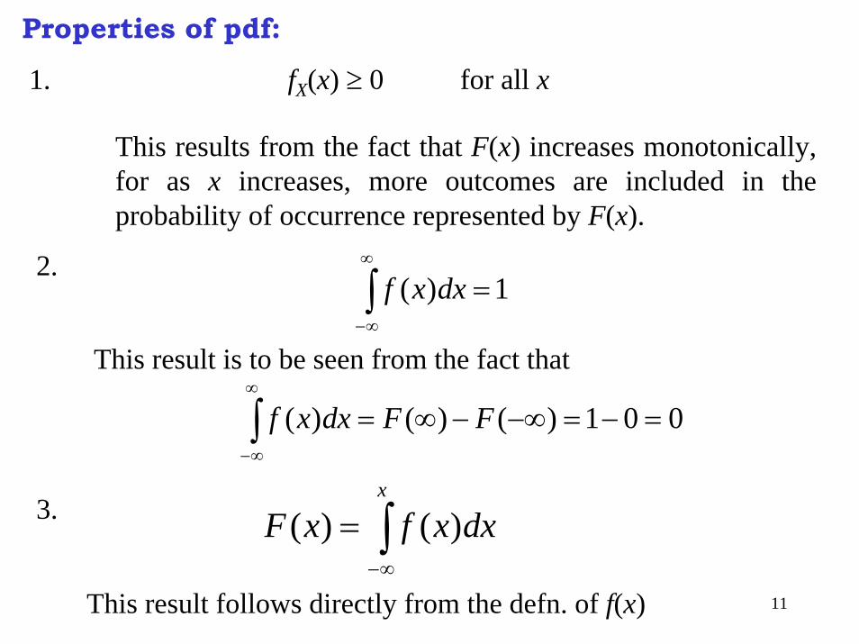
Properties of pdf:
1. fX(x) ≥ 0 for all x
This results from the fact that F(x) increases monotonically, for as x increases, more outcomes are included in the probability of occurrence represented by F(x).
2.∫∞
∞−
=1)( dxxf
This result is to be seen from the fact that
∫∞
∞−
=−=−∞−∞= 001)()()( FFdxxf
3. ∫∞−
=x
dxxfxF )()(
This result follows directly from the defn. of f(x)

12
Several Random Variables:
It may be necessary to identify the outcome of an experiment by two (or more) random variables.
Let us consider the case of two random variables X and Y.
Joint Distribution Function:
∫ ∫∞− ∞−
=
≤≤=y x
XY
XY
dxdyyxf
yYxXPyxF
),(
),(),(
The joint distribution function FXY(x,y) is defined as the probability that the random variable X is less than or equal to a specified value x and that the random variable Y is less than or equal to a specified value y.

13
Note: (i) The joint sample space is the xy-plane
(ii) FXY(x,y) is the probability that the outcome of an experiment will result in a sample point lying inside the quadrant (-∞ < X ≤ x, -∞ < Y ≤ y) of the joint sample space
Joint pdf:
The joint pdf of the random variables X and Y is defined by
provided this partial derivative exists
∫ ∫=≤≤≤≤2
1
2
1
),(),( 2121
y
y
x
xXY dxdyyxfyYyxXxP
14
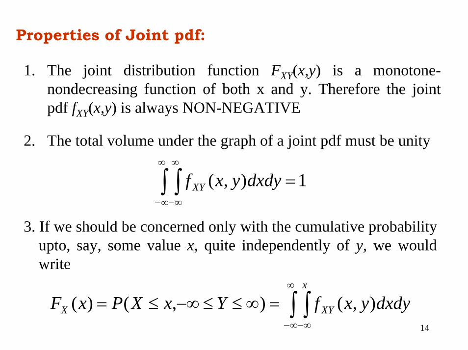
Properties of Joint pdf:
1. The joint distribution function FXY(x,y) is a monotone-nondecreasing function of both x and y. Therefore the joint pdf fXY(x,y) is always NON-NEGATIVE
1),( =∫ ∫∞
∞−
∞
∞−
dxdyyxf XY
2. The total volume under the graph of a joint pdf must be unity
∫ ∫∞
∞− ∞−
=∞≤≤−∞≤=x
XYX dxdyyxfYxXPxF ),(),()(
3. If we should be concerned only with the cumulative probability upto, say, some value x, quite independently of y, we would write
15
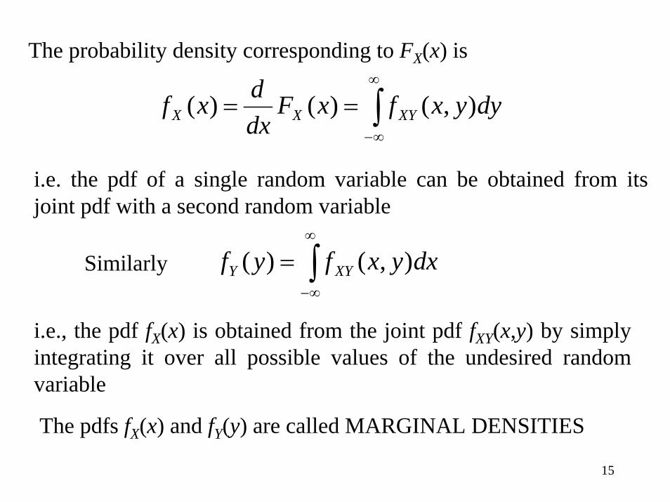
∫∞
∞−
== dyyxfxFdxdxf XYXX ),()()(
The probability density corresponding to FX(x) is
i.e. the pdf of a single random variable can be obtained from its joint pdf with a second random variable
∫∞
∞−
= dxyxfyf XYY ),()(Similarly
i.e., the pdf fX(x) is obtained from the joint pdf fXY(x,y) by simply integrating it over all possible values of the undesired random variable
The pdfs fX(x) and fY(y) are called MARGINAL DENSITIES
16
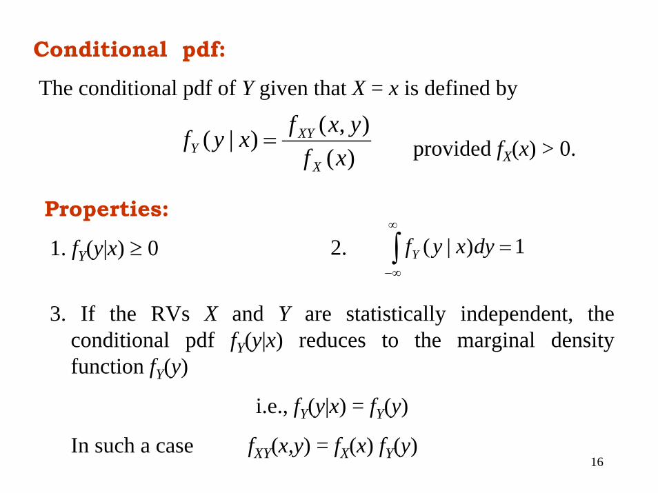
Conditional pdf:
)(),()|(
xfyxfxyf
X
XYY =
The conditional pdf of Y given that X = x is defined by
provided fX(x) > 0.
Properties:2. ∫
∞
∞−
=1)|( dyxyfY1. fY(y|x) ≥ 0
3. If the RVs X and Y are statistically independent, the conditional pdf fY(y|x) reduces to the marginal density function fY(y)
i.e., fY(y|x) = fY(y)
In such a case fXY(x,y) = fX(x) fY(y)

17
4. When X and Y are independent
⎥⎥⎦
⎤
⎢⎢⎣
⎡
⎥⎥⎦
⎤
⎢⎢⎣
⎡=≤≤≤≤ ∫∫
2
1
2
1
)()(),( 2121
y
yY
x
xX dyyfdxxfyYyxXxP

18
Statistical Average:
Let us consider the problem of determining the average height ofthe entire population of a country
If the data is recorded within the accuracy of an inch, then theheight X of every person will be approximated to one of the nnumbers x1, x2, …, xn.If there are Ni persons of height xi, then the average height is given by
NxNxNxNX nn+++
=K2211
N = total number of the persons
nn x
NNx
NNx
NNX +++= K2
21
1
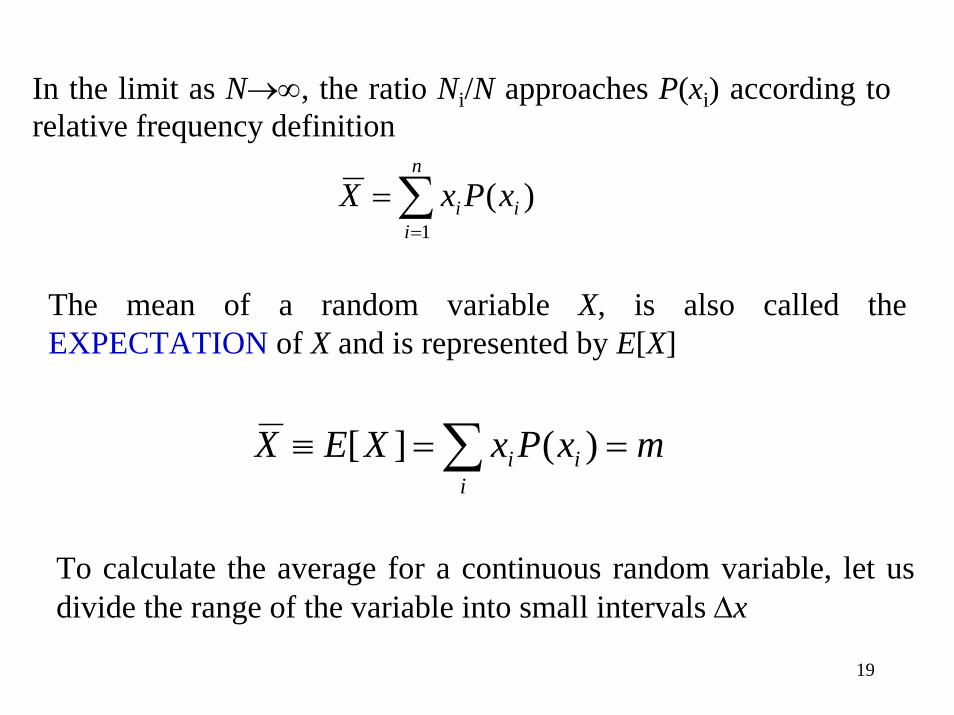
19
In the limit as N→∞, the ratio Ni/N approaches P(xi) according to relative frequency definition
∑=
=n
iii xPxX
1)(
The mean of a random variable X, is also called the EXPECTATION of X and is represented by E[X]
∑ ==≡i
ii mxPxXEX )(][
To calculate the average for a continuous random variable, let us divide the range of the variable into small intervals ∆x

20
The probability that X lies in the range between xi and xi+ ∆x is )()( iii xPxxXxP ≡∆+≤≤
is given approximately by
xxfxP ii ∆= )()(
So we have xxfxm ii
i ∆=∑ )(
In the limit, ∆x → 0, ∫∞
∞−
= dxxxfm )(
Therefore ∫∞
∞−
= dxxxfXE X )(][
21
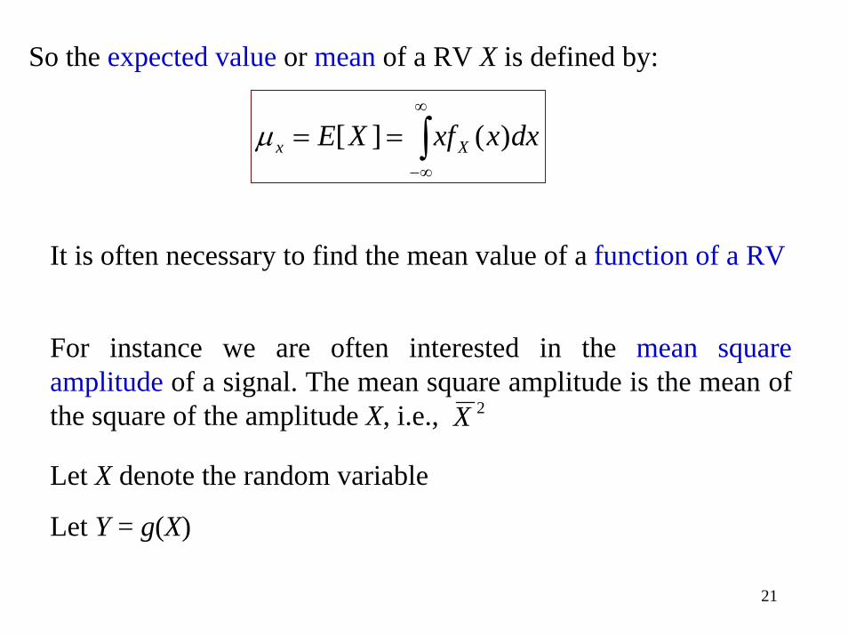
So the expected value or mean of a RV X is defined by:
∫∞
∞−
== dxxxfXE Xx )(][µ
It is often necessary to find the mean value of a function of a RV
For instance we are often interested in the mean square amplitude of a signal. The mean square amplitude is the mean of the square of the amplitude X, i.e., 2X
Let X denote the random variable
Let Y = g(X)

22
The average value, or expectation, of a function g(X) of the RV X is given by:
∫∞
∞−
= dyyyfYE Y )(][
∫∞
∞−
= dxxfxgXgE X )()()]([or
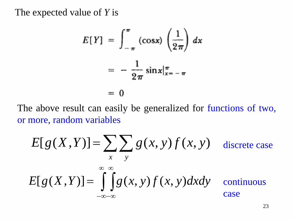
Example:
23
The expected value of Y is
The above result can easily be generalized for functions of two, or more, random variables
∑∑=x y
yxfyxgYXgE ),(),()],([ discrete case
∫ ∫∞
∞−
∞
∞−
= dxdyyxfyxgYXgE ),(),()],([ continuous case
24
∫∞
∞−
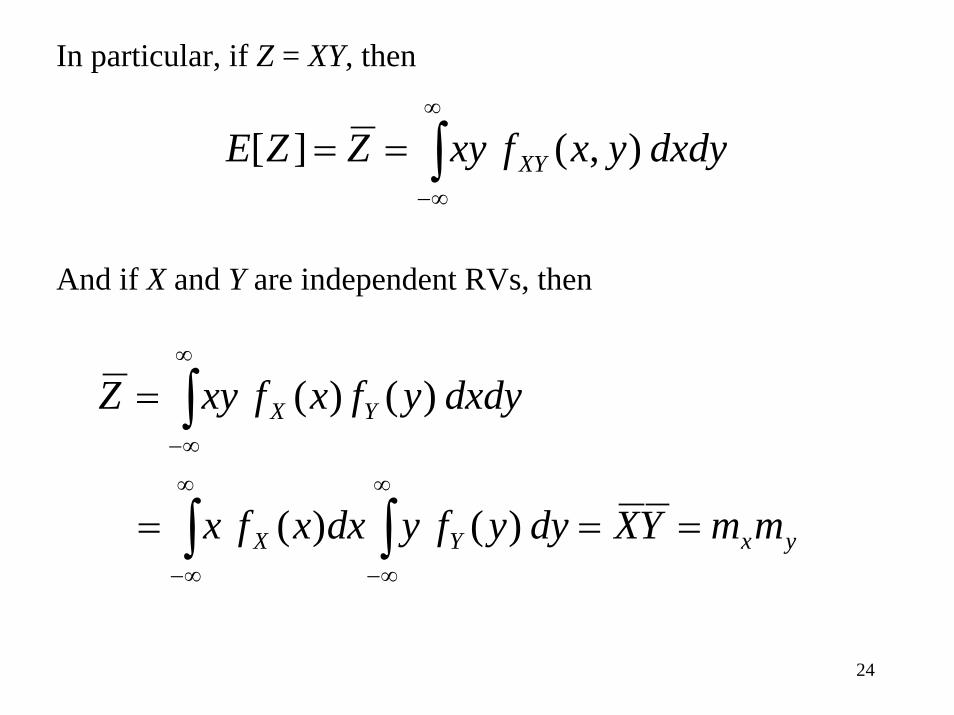
== dxdyyxfxyZZE XY ),( ][
In particular, if Z = XY, then
yxYX
YX
mmYXdyyfydxxfx
dxdyyfxfxyZ
===
=
∫ ∫
∫∞
∞−
∞
∞−
∞
∞−
)( )(
)()(
And if X and Y are independent RVs, then
25
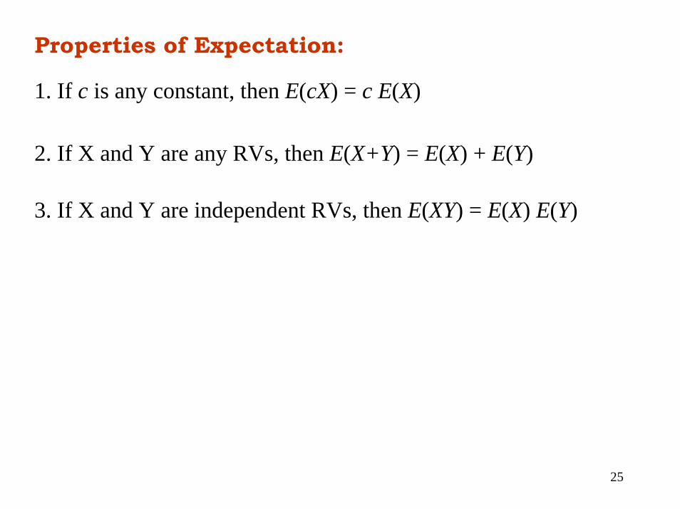
Properties of Expectation:
1. If c is any constant, then E(cX) = c E(X)
2. If X and Y are any RVs, then E(X+Y) = E(X) + E(Y)
3. If X and Y are independent RVs, then E(XY) = E(X) E(Y)

26
Moments:
If the function g(X) is X raised to a power, i.e., g(X) = Xn, the average value E[Xn] is referred to as the nth moment of the random variable
∫∞
∞−
= dxxfxXE
XX
Xnn )(][
ofmoment First :
The most important moments of X are the first two moments
n = 1: gives the mean of the random variable
∫∞
∞−
= dxxfxXE X )(][ 22
n = 2: gives the mean-square value of X
27
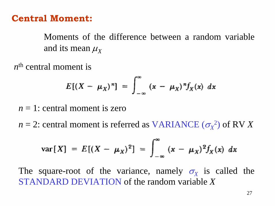
Central Moment:
Moments of the difference between a random variable and its mean µX
nth central moment is
n = 1: central moment is zero
n = 2: central moment is referred as VARIANCE (σX2) of RV X
The square-root of the variance, namely σX is called the STANDARD DEVIATION of the random variable X
28
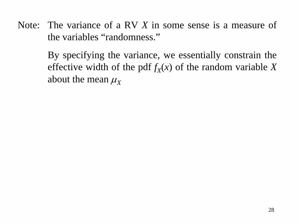
Note: The variance of a RV X in some sense is a measure of the variables “randomness.”
By specifying the variance, we essentially constrain the effective width of the pdf fX(x) of the random variable Xabout the mean µX

29
Variance and Standard Deviation
Consider two RVs, whose density functions are given by Curves I and II.
Both of them have the same mean (µ). Yet both the RVs differ in some way
That is, mean alone does not characterize a RV. To characterize a RV, we must also know how it varies or deviates from its mean

30
We may be inclined to take E(X - µ) as another characteristic of a RV to indicate its deviation, or dispersion about its mean.
Let us consider the curves I and II, to be symmetric about µ. Then (X- µ) is +ve for X > µ, and negative for X < µ, resulting in E(X- µ) = 0, in both the cases
Thus E(X- µ) does not serve our purpose. If a function treats both +ve and –ve differences identically, our purpose is served.
E(|X- µ|) and [E(X- µ)2] are two such functions. However it is found that [E(X- µ)2] is more useful function of the two.
When we interpret f(x) as the mass density on X-axis, the mean is the center of gravity of mass. Variance, equals the moment of inertia of the probability masses and gives some notion of their concentration near the mean
31
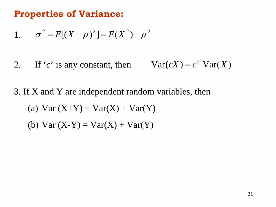
Properties of Variance:
2222 )(])[( µµσ −=−= XEXE1.
If ‘c’ is any constant, then )(Var )(Var 2 XccX =2.
3. If X and Y are independent random variables, then
(a) Var (X+Y) = Var(X) + Var(Y)
(b) Var (X-Y) = Var(X) + Var(Y)
32
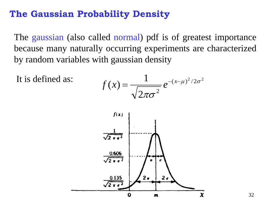
The Gaussian Probability Density
The gaussian (also called normal) pdf is of greatest importance because many naturally occurring experiments are characterized by random variables with gaussian density
22 2/)(
221)( σµ
πσ−−= xexfIt is defined as:
33
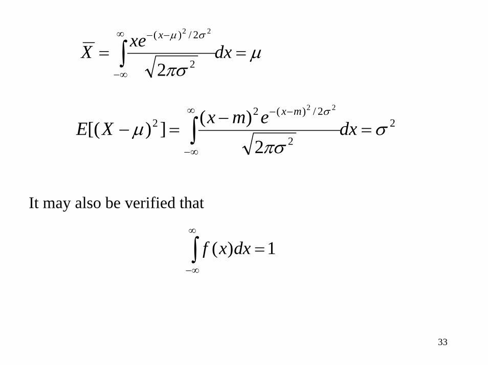
µπσ
σµ
== ∫∞
∞−
−−
dxxeXx
2
2/)(
2
22
2
2
2/)(22
2)(])[(
22
σπσ
µσ
=−
=− ∫∞
∞−
−−
dxemxXEmx
∫∞
∞−
=1)( dxxf
It may also be verified that

34
Joint Moments
The joint moment for a pair of RVs X and Y is defined by:
i, k: any +ve integers
When i = k = 1, the joint moment is called the CORRELATIONdefined by E[XY]
The correlation of the centered random variables X - E[X] and Y - E[Y] is called the COVARIANCE of X and Y
or
35
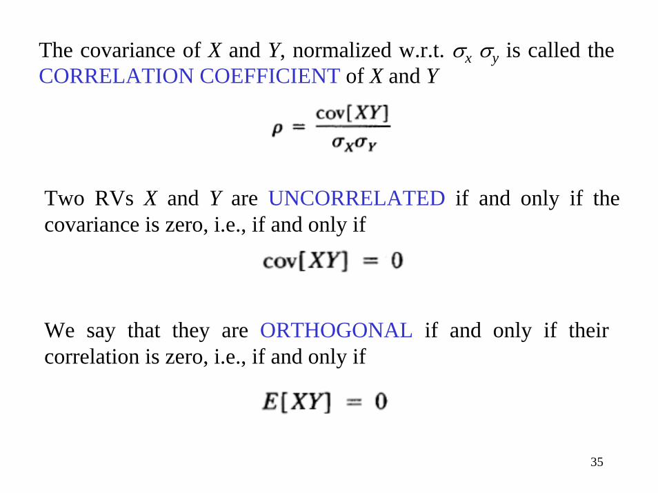
The covariance of X and Y, normalized w.r.t. σx σy is called the CORRELATION COEFFICIENT of X and Y
Two RVs X and Y are UNCORRELATED if and only if the covariance is zero, i.e., if and only if
We say that they are ORTHOGONAL if and only if their correlation is zero, i.e., if and only if

36
Transformations of RVs
Question: How to determine the pdf of a RV Y related to another RV X by the transformation Y = g(X)
Case I: Monotone (one-to-one) Transformations
(one value of x is transformed into one value of y)
Case II: Non-monotone (many-to-one) Transformations
(several values of x can be transformed into one value of y)

37
Monotone Transformations
Let X be a RV with pdf fX(x) and let Y = g(X) be a monotone differential function of X
⇒
dy is the infinitesimal change in y that occurs due to an infinitesimal change in x, i.e., dx
38
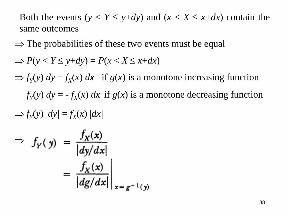
Both the events (y < Y ≤ y+dy) and (x < X ≤ x+dx) contain the same outcomes ⇒ The probabilities of these two events must be equal
⇒ P(y < Y ≤ y+dy) = P(x < X ≤ x+dx)
⇒ fY(y) dy = fX(x) dx if g(x) is a monotone increasing function
fY(y) dy = - fX(x) dx if g(x) is a monotone decreasing function
⇒ fY(y) |dy| = fX(x) |dx|
⇒

39
Many-to-one TransformationsLet the equation g(x) = y has three roots x1, x2 and x3
⇒ g(x+dx) = (y + dy) has three roots x1 + dx1, x2 + dx2, and x3+ dx3
⇒ The event (y < Y ≤ y+dy) occurs when any of the three events (x1 < X ≤ x1+dx1), (x3 < X ≤ x2+dx2), or (x3 < X ≤x3+dx3) occurs
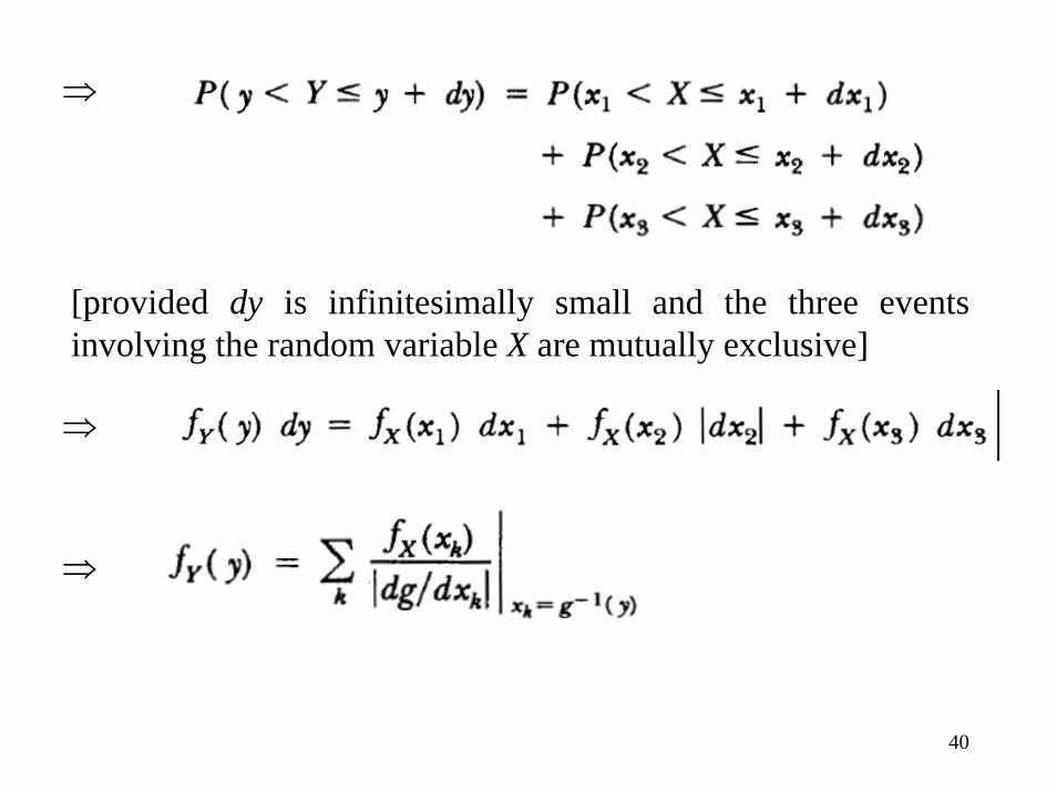
40
⇒
[provided dy is infinitesimally small and the three events involving the random variable X are mutually exclusive]
⇒
⇒

41
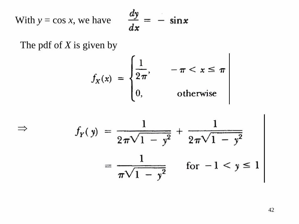
Example: Consider the transformation Y = cos X, where the RV X is uniformly distributed in the interval (-π, π). Find the pdf of Y.
Soln.: For -1 < Y ≤ 1, the equation cos x = y has two solutions, namely
42
With y = cos x, we have
The pdf of X is given by
⇒


